a determination of optimal ship forms based on michell's...

A determination of optimal ship forms based

on Michell’s wave resistance

Morgan PIERRE

Laboratoire de Mathematiques et Applications, UMR CNRS 7348,

Universite de Poitiers, France

Benasque, August 26th 2015with J. Dambrine (LMA Poitiers) and G. Rousseaux (Pprime

Institute, Poitiers)

Outline

1 Michell’s wave resistance formula

2 Formulation of the optimization problem

3 Theoretical results

4 Numerical results

5 About the case ǫ = 0

6 Conclusion and perspectives

Michell’s wave resistance formulaFormulation of the optimization problem

Theoretical resultsNumerical results

About the case ǫ = 0Conclusion and perspectives

Traditionally, the resistance of water to the motion of a ship isrepresented as

Rwater = Rwave + Rviscous ,

withRviscous = Rfrictional + Reddy .

Morgan PIERRE Optimal ship forms

(AFP / N. Lambert photography)

( Shutterstock.com/ AlexKol photography)




Consider a ship moving with constant velocity U on the surface ofan unbounded fluid.

coordinates xyz are fixed to the ship

the xy -plane is the water surface, z is vertically downward

The (half-)immerged hull surface is represented by a continuousnonnegative function

y = f (x , z) ≥ 0, x ∈ [−L/2, L/2], z ∈ [0,T ],

where L is the length and T is the draft of the ship. We alsoassume

f (±L/2, z) = 0 ∀z and f (x ,T ) = 0 ∀x .





Example: for a Wigley hull with beam B , we havef (x , z) = (B/2)S(z)(1− 4x2/L2) with

S(z) =

1− (z/T )2 (parabolic cross section)

1− z/T (triangular cross section)

1 (rectangular cross section).





Michell’s formula (1898) reads:

RMichell =4ρg2

πU2

∫

∞

1

(I (λ)2 + J(λ)2)λ2

√λ2 − 1

dλ, (1)

with

I (λ) =

∫ L/2

−L/2

∫ T

0

∂f (x , z)

∂xexp

(

−λ2gz

U2

)

cos

(

λgx

U2

)

dxdz , (2)

J(λ) =

∫ L/2

−L/2

∫ T

0

∂f (x , z)

∂xexp

(

−λ2gz

U2

)

sin

(

λgx

U2

)

dxdz . (3)





U (in m · s−1) is the speed of the ship

ρ (in kg ·m−3) is the (constant) density of the fluid

g (in m · s−2) is the standard gravity.

RMichell has the dimension of a force. λ has no dimension andλ = 1/ cos θ where θ is the angle at which the wave is propagating.





The fluid is incompressible, inviscid, the flow is irrotational

A steady state has been reached

Linearized theory (flow potential with linearized boundaryconditions)

Thin ship assumptions: |∂x f | << 1, |∂z f | << 1.

Experiments starting in the 1920’s (Wigley, Weinblum):reasonable good agreement between theory and experiment(Gotman’02). Typical values for Wigley: L/B ≈ 10 andT/B = 1.5.

The following figures represent the wave coefficientCW = 2Rwave/(ρU

2A) (with A the wetted surface of the hull) interms of the Froude number F = U/

√gL.





Comparison Michell and experimental data (Weinblum’52)





Comparison Michell and experimental data (parabolic Wigley model, Bai’79)





Derivation of Michell’s formula (sketch)

In the coordinates xyz fixed to the ship, we have U = −U + u,where u is the perturbed velocity flow. We seek a potential flow Φ(i.e. with u = ∇Φ), even with respect to y , which satisfies inD = Rx × (R+)y × (R+)z :

∆Φ = 0 in D (4)

∂xxΦ− (g/U2)∂zΦ = 0, z = 0 (5)

∂yΦ = −Ufx , y = 0+ (6)

∇Φ → 0 as x → +∞. (7)

Φ can be computed explicitly by means of Green functions andFourier transform.





Let Ω = (−L/2, L/2)× (0,T ). Then the wave resistance reads

Rwave = −2

∫

Ω

δpfx(x , z)dxdz ,

where δp is the difference of pressure due to the ship. (Notice thatRwave is the drag force in this linearized model).From Φ, we derive δp so that

Rwave = −2ρU

∫

Ω

Φx(x , 0, z)fx(x , z)dxdz .

Computing, we obtain Rwave = RMichell as given by (1).





Formulation of the optimization problem

1st idea: finding a ship of minimal wave resistance amongadmissible functions f : Ω → R+, for a constant speed U and agiven volume V of the hull.f 7→ RMichell(f ) is a positive semi-definite quadratic functional, butthe problem above is ill-posed (Sretensky’35, Krein’52). Inparticular, it is underdetermined.

Most authors proposed to add conditions and/or to work in finitedimension (Weinblum’56, Kostyukov’68,. . . )Another approach, that we chose: add a regularizing term whichrepresents the viscous resistance (Lian-en’84, Michalski et al’87)





We define

v = g/U2 > 0 and Tf (v , λ) = I (λ)− iJ(λ),

where I and J are given by (2)-(3). Then

Tf (v , λ) =

∫ L/2

−L/2

∫ T

0

∂x f (x , z)e−λ2vze−iλvxdxdz , (8)

and RMichell can be written

R(v , f ) =4ρgv

π

∫

∞

1

|Tf (v , λ)|2λ2

√λ2 − 1

dλ. (9)





For the numerical computation, we let Λ >> 1 and consider

RΛ(v , f ) =4ρgv

π

∫ Λ

1

|Tf (v , λ)|2 dµ(λ), (10)

where µ is a nonnegative and finite borelian measure on [1,Λ].Typically,

dµ(λ) =λ2

√λ2 − 1

dλ,

or a numerical integration of this weight.


For the viscous resistance, we propose

Rviscous =1

2ρU2CvdA,

where Cvd is the (constant) viscous drag coefficient, and A is thewetted surface area given by

A = 2

∫

Ω

√

1 + |∇f (x , z)|2 dxdz .

For instance, the ITTC 1957 model-ship correlation line gives

Cvd = 0.075/(log10(Re)− 2)2,

where Re = UL/ν is the Reynolds number and ν the kinematicviscosity of water.For small ∇f (thin ship assumption)

Rviscous ≈ ρU2 Cvd

(∫

Ω

dxdz +1

2

∫

Ω

|∇f (x , z)|2 dxdz)

.




By setting

ǫ =1

2ρU2 Cvd , (11)

and dropping the constant term, we obtain

R∗

viscous = ǫ

∫

Ω

|∇f (x , z)|2 dxdz .

The total water resistance functional NΛ,ǫ(v , ·) is

NΛ,ǫ(v , f ) := RΛ(v , f ) + ǫ

∫

Ω

|∇f (x , z)|2dxdz .





The function space is

H =

f ∈ H1(Ω) : f (±L/2, ·) = 0 and f (·,T ) = 0 a.e.

,

Let V > 0 be the (half-)volume of an immerged hull. The set ofadmissible functions is

CV =

f ∈ H :

∫

Ω

f (x , z)dxdz = V and f ≥ 0 a.e. in Ω

.

Notice that CV is a closed convex subset of H.NB: the volume is proportional to the displacement of the ship.





The optimization problem

Our optimization problem PΛ,ǫ reads: for a given Kelvin wavenumber v and for a given volume V > 0, find the function f ⋆

which minimizes the total resistance NΛ,ǫ(v , f ) among functionsf ∈ CV .Recall that

NΛ,ǫ(v , f ) := RΛ(v , f ) + ǫ

∫

Ω

|∇f (x , z)|2dxdz

andv = g/U2.

In short, “minimize the (total) drag for a given displacement”.





Well-posedness

The parameters ρ > 0, g > 0, V > 0, Λ > 0, v > 0 and ǫ > 0 arefixed (unless otherwise stated).

Theorem (Dambrine, P. & Rousseaux (to appear))

Problem PΛ,ǫ has a unique solution f ǫ,v ∈ CV . Moreover, f ǫ,v is

even with respect to x.

Existence by a minimizing sequence

Uniqueness by strict convexity

Symmetry thanks to the symmetry of RMichell throughx 7→ −x .

Remark: also valid if Λ = ∞ with RMichell instead of RΛ.





Continuity of the optimum with respect to v


Let v > 0. Then f ǫ,v converges strongly in H to f ǫ,v as v → v .

idea of proof

NΛ,ǫ(v , ·) Γ-converges to NΛ,ǫ(v , ·) for the weak topology inH, thanks to Λ < ∞.

strong convergence thanks to the convergence of the H1-norm

Remark: result also valid if ǫ > 0 depends continuously on v .





Regularity of the solution


The solution f ǫ,v of problem PΛ,ǫ belongs to W 2,p(Ω) for all1 ≤ p < ∞. In particular, f ǫ,v ∈ C 1(Ω).





Sketch of proof (regularity)

The problem is a perturbation of an obstacle-type problem for theDirichlet energy

The Euler-Lagrange equation gives a variational inequality foran obstacle-type problem

By a standard result, the regularity of the obstacle problem isgiven by the regularity of unconstrained problem

The unconstrained problem reads −∆f ǫ,v = w withw ∈ L∞(Ω), and homogeneous Dirichlet BC on 3 sides +no-flux BC on 1 side of the rectangle, hence f ǫ,v ∈ W 2,p(Ω)for all 1 ≤ p < ∞.





Numerical methods

Q1 finite element discretization of the space H

the integrals

J(λ) =

∫ L/2

−L/2

∫ T

0

∂f (x , z)

∂xexp

(

−λ2gz

U2

)

sin

(

λgx

U2

)

dxdz .

(12)are computed exactly on the basis functions

the antisymmetric contribution I (λ) is dropped (since theminimizer is even with respect to x).

for the last integral RMichell , we use a midpoint formula whichpreserves nonnegativity of the quadratic form + Tarafder’strick to improve accuracy

Uzawa algorithm for the resolution





Numerical test

ρ = 1000 kg ·m−3, g = 9.81m · s−2, L = 2m, T = 20 cm,V = 0.03m3.

Nx = 100 and Nz = 20

ǫ = 12ρCvdU

2 with Cvd = 0.01

Fr = U/√gL





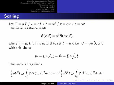
Scaling

Let T = αT / L = αL / f = αf / x = αx / z = αzThe wave resistance reads

R(v , f ) = α3R(αv , f ),

where v = g/U2. It is natural to set v = αv , i.e. U =√αU, and

with this choice,

Fr = U/√

gL = Fr = U/

√

gL.

The viscous drag reads

1

2ρU2Cvd

∫

Ω

|∇f (x , z)|2dxdz = α3 1

2ρU2Cvd

∫

Ω

|∇f (x , z)|2dxdz .


−1

−0.8

−0.6

−0.4

−0.2

0

0.2

0.4

0.6

0.8

1

−0.10

0.1

−0.2

−0.1

0

No waveresistance

−1

−0.8

−0.6

−0.4

−0.2

0

0.2

0.4

0.6

0.8

1

−0.10

0.1

−0.2

−0.1

0

Fr =0.1

−1

−0.8

−0.6

−0.4

−0.2

0

0.2

0.4

0.6

0.8

1

−0.10

0.1

−0.2

−0.1

0

Fr =0.2

−1

−0.8

−0.6

−0.4

−0.2

0

0.2

0.4

0.6

0.8

1

−0.10

0.1

−0.2

−0.1

0

Fr =0.3

−1

−0.8

−0.6

−0.4

−0.2

0

0.2

0.4

0.6

0.8

1

−0.10

0.1

−0.2

−0.1

0

Fr =0.4

−1

−0.8

−0.6

−0.4

−0.2

0

0.2

0.4

0.6

0.8

1

−0.10

0.1

−0.2

−0.1

0

Fr =0.5

−1

−0.8

−0.6

−0.4

−0.2

0

0.2

0.4

0.6

0.8

1

−0.10

0.1

−0.2

−0.1

0

Fr =0.6

−1

−0.8

−0.6

−0.4

−0.2

0

0.2

0.4

0.6

0.8

1

−0.10

0.1

−0.2

−0.1

0

Fr =0.7

−1

−0.8

−0.6

−0.4

−0.2

0

0.2

0.4

0.6

0.8

1

−0.10

0.1

−0.2

−0.1

0

Fr =1.5

−1

−0.8

−0.6

−0.4

−0.2

0

0.2

0.4

0.6

0.8

1

−0.10

0.1

−0.2

−0.1

0

Fr =2

The bulbous bow of “Harmony of the Seas” (AFP / G. Gobet photo)Speed : 20 knots / Length : 362m / Fr=0.17 (/T=9.1m / B=47m)

ITTC 1957 gives Cvd = 0.0013




0.1 0.2 0.3 0.4 0.5 0.6 0.7 0.8 0.90

10

20

30

40

50

60

Froude number

Wav

e re

sist

ance

Wigley Hull

Optimized for Fr = 0.5

Comparison with a Wigley hull





About the case ǫ = 0

In this section, we assume

RΛ(v , f ) =4ρgv

π

∫ Λ

1

|Tf (v , λ)|2λ2

√λ2 − 1

dλ,

with 1 < Λ ≤ ∞ (i.e. “true” Michell wave resistance, or truncatedMichell wave resistance).

Proposition (Krein’52)

Let v > 0. For all f ∈ CV , RΛ(v , f ) > 0. More precisely,

inff ∈CV

RΛ(v , f ) > 0.

⇒ There is no ship with wave resistance equal to 0.





However, this is possible if L = ∞ (endless caravan of ships).Indeed, choose

f (x , z) = g(x)h(z), g(x) =sin2(ax)

ax2

and h arbitrary. Then for v < a, Tf (v , λ) = 0 for all λ ≥ 1 and soRΛ(v , f ) = 0.

Moreover, if L < ∞ , for any h ∈ C∞

c (Ω), by settingf = ∂2

xh + v∂zh, we have by integration by parts:

Tf (v , λ) = iλv

∫ L/2

−L/2

∫ T

0

f (x , z)e−λ2vze−iλvxdxdz = 0,

and soRΛ(v , f ) = 0.

(but in this case, f changes sign !)Morgan PIERRE Optimal ship forms

0 200 400 600 800 1000 1200 1400 160010

−20

10−15

10−10

10−5

100

105

i

λ

Figure: Eigenvalues of Mw ≈ RΛ for a 100× 30 grid




Letting ǫ → 0

Proposition (Dambrine, P. & Rousseaux (to appear))

The minimum value NΛ,ǫ(v , f ǫ,v ) tends to

mΛ,v := inff ∈CV

RΛ(v , f )

as ǫ tends to 0.

Remark: Up to a subsequence, f ǫ,v tends to a finite nonnegativemeasure with support in Ω, weakly-⋆ in (C (Ω))′.


ε=0.01

−1 −0.5 0 0.5 1

0

0.1

0.2

ε=0.0025

−1 −0.5 0 0.5 1

0

0.1

0.2

ε=0.000625

−1 −0.5 0 0.5 1

0

0.1

0.2

ε=0.00015625

−1 −0.5 0 0.5 1

0

0.1

0.2

Figure: Color maps of the optimized hull function f (x , z) for smaller andsmaller values of ǫ.




The one dimensional case

For simplicity, we restrict the study to the functions f (x , z) = f (x)with infinite draft T . Moreover, f (±L/2) = 0 and by symmetry, fis even. Then (for Λ = ∞),

RMichell =4ρgv

π

∫

∞

1

Sf (v , λ)2 1√

λ2 − 1dλ

with

Sf (v , λ) =

∫ L/2

−L/2f (x) cos(λvx)dx . (13)

We minimize RMichell in

CV := f ∈ H10 (−L/2, L/2) : f even,

∫ L/2

−L/2f = V , f ≥ 0 a.e..





Proposition (1d case)

Any minimizing sequence (fn) converges to the same finite

nonnegative measure µv on [−L/2, L/2]. Moreover, µv belongs to

H−1/2(−L/2, L/2).

Uniqueness: Sf is the Fourier transform of f , so by analycity,RMichell is a norm on L2(−L/2, L/2), which has a natural l.s.c.extension to a norm on (C ([−L/2, L/2])′.Estimate: use Fatou’s lemma and the standard definition ofH−1/2(R) by Fourier transform. Indeed,

H−1/2(R) := g ∈ S ′(R) :

∫

R(1 + λ2)−1/2|g(λ)|2dλ < ∞.


Solution for ǫ = 1, ǫ = 0.05 and ǫ = 0.01 (Fr = 0.4)




1d Resolution without positivity condition (Krein’52)

If we suppress the positivity condition, then the minimizationproblem is quadratic with linear constraint. The Euler-Lagrangeequation reads: find f : I → R s.t.

∫

I

Kv (x − ξ)f (ξ)dξ = cst, ∀x ∈ I , (14)

where I = (−L/2, L/2) and

Kv (x − ξ) =

∫

∞

1

cos(λv(x − ξ))√λ2 − 1

dλ.

This is a Fredholm integral equation of the first kind. Well-knowncategory of ill-posed problems !





We haveKv (x) = cv ln(1/|x |) + g(x),

where g is continuously differentiable on I and twice continuouslydifferentiable on I \ 0.Keeping only the first term of Kv in (14), the solution is given by

f (x) =C

√

(L/2)2 − x2,

where C is a constant.Singularity at x = ±L/2. In particular, f 6∈ H1(I ).





A numerical experiment (1d)

Discretization of the Euler-Lagrange equation (14) by P1 finiteelement in H1(−L/2, L/2), and its ǫ-regularized version (Tykhonovregularization).Fr = 0.4 (L = 3 / V = 0.1)N = number of degrees of freedomκ = condition number of the (augmented) linear system


Condition number vs degrees of freedom (1d)




Conclusion and perspectives

Other formulasMichell assumes an unbounded domain, i.e. depth H = ∞ andwidth W = ∞. There are also integral formulas for:

H = ∞ and W < ∞ (Sretensky’36)

H < ∞ and W = ∞ (Sretensky’37)

H < ∞ and W < ∞ (Sretensky’37 and Keldish-Sedov’37)

Multilayers (dead-water effects) . . .


Wave resistance of a Wigley hull for 3 different domains




Fixed speed U ⇒ range of speeds

fixed domain of parameters ⇒ varying domain (shapeoptimization)

. . .





Thank you for your attention !


a determination of optimal ship forms based on michell's...

Documents