determination of optimal forging conditions for void
TRANSCRIPT

DETERMINATION OF OPTIMAL FORGING CONDITIONS FOR VOID ELIMINATION IN LARGE
STEEL INGOTS
by
Nathan HARRIS
MANUSCRIPT-BASED THESIS PRESENTED TO ÉCOLE DE TECHNOLOGIE SUPÉRIEURE IN PARTIAL FULFILLMENT
OF THE REQUIREMENTS FOR THE DEGREE OF MECHANICAL ENGINEERING
M.A.Sc
MONTREAL, SEPTEMBER, 07 2016
ÉCOLE DE TECHNOLOGIE SUPÉRIEURE UNIVERSITÉ DU QUÉBEC
Nathan Harris, 2016

This Creative Commons licence allows readers to download this work and share it with others as long as the
author is credited. The content of this work may not be modified in any way or used commercially.

BOARD OF EXAMINERS
THIS THESIS HAS BEEN EVALUATED
BY THE FOLLOWING BOARD OF EXAMINERS Mr. Mohammad Jahazi, Thesis Supervisor Department of Mechanical Engineering at École de technologie supérieure Mr. Patrick Terriault, Chair, Board of Examiners Department of Mechanical Engineering at École de technologie supérieure Pierre Belanger, Member of the jury Department of Mechanical Engineering at École de technologie supérieure Mr. Louis-Philippe Lapierre Boire, External Evaluator Sorel Forge
THIS THESIS WAS PRENSENTED AND DEFENDED
IN THE PRESENCE OF A BOARD OF EXAMINERS AND THE PUBLIC
SEPTEMBER 07, 2016
AT ÉCOLE DE TECHNOLOGIE SUPÉRIEURE


ACKNOWLEDGMENTS
The author would like to thank M.A.Sc research director, Mohammad Jahazi, for his
guidance, support and expertise during the degree, without which none of this would have
been possible. Gratitude is also expressed for Davood Shahriari, ETS, research assistant, for
his cooperation the entire duration of the diploma.
Thanks are given to Industrial Partner, Finkl Steel, and in particular Louis Philippe Lapierre
Boire, for his complete collaboration in the organisation of this project and a corresponding
internship accomplished during January and February 2016. Special thanks are given again to
Louis Philippe for transportation and carpooling throughout the entire internship.
Appreciation is accorded for time granted off campus in this endeavour.
Gratitude is acknowledged for the Sorel Forge team, notably Rami Tremblay, Jean Benoit
Morin and Stephane Roy for their help in accessing Sorel Forge information points and
sample preparation. Finally, thanks are given to the forging teams especially Mario for his
kind welcome and enthusiasm to assist.


DÉTERMINATION DES CONDITIONS OPTIMALES POUR L’ÉLIMINATION
DES POROSITÉS LORS DE LA MISE EN FORME DES LINGOTS D’ACIER DE
GRANDE TAILLE
Nathan HARRIS
RÉSUMÉ
La présence de porosités et de cavités internes est habituellement observée lors de la coulée et de la solidification des lingots de grande taille. Leur élimination et fermeture mécanique est réalisée pendant les premières déformations du procédé de transformation à chaud. Ce travail vise à déterminer les conditions optimales pour l’élimination des porosités dans des lingots de grande taille avec une attention spéciale portée au matériau et au procédé industriel utilisé. Un état de l’art présente les modèles de fermeture de porosités et les techniques de caractérisation existantes. Actuellement, il est montré que cette théorie est très peu appliquée aux lingots utilisés en industrie. Une analyse du procédé de forgeage du partenaire industriel est effectuée et différentes séquences de forgeage sont identifiées. Ensuite, une étude plus poussée utilisant des données expérimentales est proposée. Une nouvelle méthode pour le développement de modèles de fermeture de porosité est énoncée. Sur la base de cette méthode, un quotient de fonctions polynomiales est établi pour le calcul des constants matériaux. L’influence de la triaxialité et des paramètres du matériau est évaluée grâce à une cartographie 3D. Le modèle de fermeture des porosités est validé pour les aciers à hautes performances mécaniques du partenaire industriel. La fermeture des porosités est évaluée pour une séquence du forgeage libre. L’effet du positionnement des porosités est étudié. L’efficacité de la séquence de forgeage pour la fermeture des porosités est caractérisée par zone. Une combinaison originale de la fermeture relative et la vitesse de déformation volumétrique permet l’optimisation du procédé de forgeage. Un nouveau logiciel pour le forgeage libre de « slab », Forge Calculus, est développé et testé avec beaucoup de données expérimentales. Le développement à venir et notamment une prédiction de la qualité de la pièce en temps réel pendant le forgeage est discutée. Mots-clés : forgeage libre, porosités, optimisation, simulation


DETERMINATION OF OPTIMAL FORGING CONDITIONS FOR VOID ELIMINATION IN LARGE STEEL INGOTS
Nathan HARRIS
ABSTRACT
The presence of internal voids is commonly observed throughout the casting and solidification of large size ingots. Their mechanical closure is generally achieved during the initial deformation of a hot forming process. The present work focuses on the determination of optimal forging conditions for void elimination in large steel ingots with respect to the involved materials and industrial processes. A state of the art is compiled as initial research in order to develop a solid background in void elimination theory. An extensive review of void closure models is presented and characterisation techniques are discussed. It is shown that current void closure models lack application to industrial scale forgings. An analysis of the industrial partner’s open die forging procedure ensues and characteristic forging sequences are introduced. Feasibility for further forging analysis using experimental data is evaluated and successfully proposed. A novel method for fast calculating void closure models is developed. Rational polynomial functions are established for the calculation of material dependant constants. 3D mapping is used to evaluate the influence of the triaxiality state and material parameters. The void closure model is validated for use on high strength steels from the industrial partner. Void closure is modeled and simulated during an open die forging sequence. The effect of in-billet void positioning is studied and the forging sequence effectiveness for void closure is validated and characterized for different zones. An original combination of data from relative void closure and volumetric strain rate provides a way for forging optimisation. Novel software for successful open die slab forging, Forge Calculus, is developed based on large amounts of experimental data. The in-house code provides fundamental information for setting forging standards. Future development concerning real time prediction of forging quality is discussed.
Keywords: open die forging, void elimination, optimisation, simulation


TABLE OF CONTENTS
Page
INTRODUCTION .....................................................................................................................1
CHAPTER 1 STATE OF THE ART ................................................................................5 1.1 Introduction ....................................................................................................................5 1.2 A modern day scale ........................................................................................................5
1.2.1 Macroscopics .............................................................................................. 6 1.2.2 Microanalytics ............................................................................................. 7 1.2.3 Mesoscopics ................................................................................................ 8
1.3 Void physics...................................................................................................................9 1.3.1 Void origins ................................................................................................ 9 1.3.2 Void geometries ........................................................................................ 11
1.3.2.1 Simplified geometry (sphere, cylinder) ..................................... 12 1.3.2.2 Equivalent ellipsoids .................................................................. 12
1.4 Influence of hot forging on void closure ......................................................................14 1.4.1 Principal hot forging techniques ............................................................... 14
1.4.1.1 Upsetting .................................................................................... 15 1.4.1.2 Cogging ...................................................................................... 16
1.4.2 Influential material and process parameters ............................................. 16 1.4.3 Material behaviour during void closure .................................................... 17
1.4.3.1 Local thermodynamic conditions in the workpiece ................... 17 1.4.3.2 Effect on the local microstructure .............................................. 19 1.4.3.3 Healing ....................................................................................... 20
1.5 Comparison of existing void closure models ...............................................................21 1.5.1 STB model ................................................................................................ 21 1.5.2 Ragabs derived work of the Gurson-Tvergaard model ............................. 22 1.5.3 Budiansky’s model.................................................................................... 23 1.5.4 Duva and Hutchinsons modified model .................................................... 24 1.5.5 Zhang and Cui’s analytical model ............................................................ 25 1.5.6 Zhang’s semi-analytical model ................................................................. 26 1.5.7 Saby’s CICAPORO model ....................................................................... 28
1.6 Characterisation techniques .........................................................................................29 1.6.1 Traditional void characterisation .............................................................. 29 1.6.2 Microtomography ..................................................................................... 30
1.6.2.1 3D microtomography ................................................................. 30 1.6.2.2 X-Ray microtomography ........................................................... 31 1.6.2.3 Synchrotron X-Ray microtomography ...................................... 32
1.6.3 3D Reconstruction software ...................................................................... 33
CHAPTER 2 PRELIMARY ANALYSIS OF THE OPEN DIE FORGING PROCESS ..................................................................................................35
2.1 Industrial partner and process selection .......................................................................35

XII
2.2 Forging sequence identification ...................................................................................36 2.2.1 Sequence 0: Initial forming ....................................................................... 37 2.2.2 Sequence 1: Upsetting............................................................................... 37 2.2.3 Sequence 2: FM process ........................................................................... 38 2.2.4 Sequence 3: Cogging ................................................................................ 39 2.2.5 Sequence 4: Finishing ............................................................................... 40
2.3 Process variability observation ....................................................................................40 2.4 Preliminary analysis .....................................................................................................42
2.4.1 Data collection .......................................................................................... 42 2.4.2 Forging sequence characterisation ............................................................ 43
2.5 Preliminary conclusions ...............................................................................................48
CHAPTER 3 DEVELOPMENT OF A FAST CONVERGING MATERIAL SPECIFIC VOID CLOSURE MODEL DURING INGOT FORGING ....51
3.1 Abstract ........................................................................................................................53 3.2 Introduction ..................................................................................................................53 3.3 Mechanical and material conditions ............................................................................56
3.3.1 Ingot breakdown process .......................................................................... 56 3.3.2 Stress and material behaviour assumptions .............................................. 57
3.4 Determination of material dependant void closure constants ......................................59 3.4.1 Development of material dependant model constant functions ................ 62
3.5 Results and discussion .................................................................................................69 3.5.1 Evolution of void closure .......................................................................... 69 Void closure model comparison ................................................................................ 72 3.5.2 Influence of the triaxiality state ................................................................ 74 3.5.3 Influence of material parameters .............................................................. 75 3.5.4 Characteristics of the investigated alloy ................................................... 76 3.5.5 Material sensitivity.................................................................................... 77
3.6 Model validation for large size ingots based on experimental observations ...............79 3.6.1 FEM simulation setup ............................................................................... 79 3.6.2 In ingot sensor positioning ........................................................................ 80 3.6.3 Stress and strain evaluation ....................................................................... 82 3.6.4 Simulation results...................................................................................... 84
3.7 Conclusions ..................................................................................................................85 3.8 Acknowledgements ......................................................................................................85 3.9 References ....................................................................................................................86
CHAPTER 4 ANALYSIS OF VOID CLOSURE DURING OPEN DIE FORGING .....89 4.1 Abstract ........................................................................................................................91 4.2 Introduction ..................................................................................................................92 4.3 Finite element analysis .................................................................................................93
4.3.1 Finite element model ................................................................................. 94 4.3.2 Rheological material model ...................................................................... 95 4.3.3 Void closure model ................................................................................... 96 4.3.4 Definition of virtual existing voids ........................................................... 96

XIII
4.4 Results and discussion .................................................................................................97 4.4.1 Void closure calculation method .............................................................. 97 4.4.2 FE results .................................................................................................. 98 4.4.3 Void closure analysis ................................................................................ 99
4.5 Conclusion .................................................................................................................101 4.6 Acknowledgements ....................................................................................................101 4.7 References ..................................................................................................................102
CHAPTER 5 DEVELOPMENT OF A PREDICTION TOOL FOR SUCCESFUL FORGING ................................................................................................105
5.1 Forge Calculus – prediction tool ................................................................................105 5.1.1 In depth analysis of successful forgings ................................................. 106
5.1.1.1 Sequence models ...................................................................... 107 5.1.1.2 Sequence algorithms ................................................................ 112 5.1.1.3 Example of application ............................................................ 116
5.1.2 Individual results module ........................................................................ 126 5.1.3 Statistical analysis module ...................................................................... 127
5.2 Future development ...................................................................................................128
CONCLUSIONS....................................................................................................................129
APPENDIX I Forging plan example ...................................................................................131
APPENDIX II Main Database Structure .............................................................................133
APPENDIX III Probability function list ..............................................................................135
BIBLIOGRAPHY ..................................................................................................................137


LIST OF TABLES
Page Table 1: Summary of presented void closure models .............................................21
Table 2: Values for the coefficient c1,c2 in Hutchison’s formula taken from Zhang and Cui (2009) .......................................................................24
Table 3: Values for the coefficients c1,c2,c3,c4 in Zhang's equation taken from Zhang et al. (2009) ...........................................................................28
Table 4 : Indicators of process variability .................................................................41
Table 5 : Raleigh Ritz calculated values for c1,c2 .....................................................64
Table 6 : Raleigh Ritz calculated values for q1,q2,q3,q4 ............................................64
Table 7 : Relative error and statistical data verification index values ......................64
Table 8 : Value of j in equation (3.8) for calculated coefficients .............................65
Table 9 : Numerator coefficient values used in equation (3.9) .................................66
Table 10 : Denominator coefficient values used in equation (3.9) .............................66
Table 11 : 3D mapping for material dependant void closure models .........................70
Table 12 : P20 chemical composition (%wt) ..............................................................77
Table 13 : Sensor positioning in billet ........................................................................82
Table 14 : Chemical composition of P20 (%wt) .........................................................95
Table 15 : Characteristic Ingot Regions ......................................................................97
Table 16 : Void closure effectiveness per axis ..........................................................100
Table 17 : Upset results per hit of anvil ....................................................................120
Table 18 : FM results per hit of anvil ........................................................................121
Table 19 : Average Upset and FM indicators ...........................................................121
Table 20 : Cogging and Finishing average indicators ...............................................126
Table 21 : Cogging and Finishing anvil blow distribution .......................................126

XVI

LIST OF FIGURES
Page
Figure 1 : Mesoscopic approach to modelling voids in large ingots taken from
(X. Zhang, 2008) ..........................................................................................9
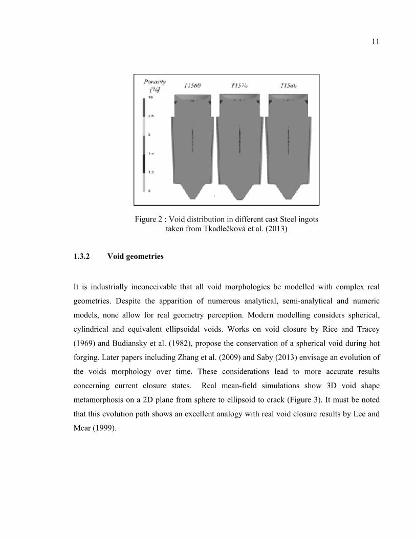
Figure 2 : Void distribution in different cast Steel ingots taken from Tkadlečková et al. (2013) ................................................................................................11
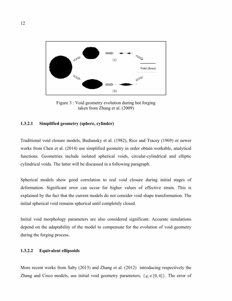
Figure 3 : Void geometry evolution during hot forging taken from Zhang et al. (2009) .........................................................................................................12
Figure 4: Definition of the dimensions and orientation of an ellipsoid taken from (M. Saby, 2013) .........................................................................................13
Figure 5 : (From left to right) Transformation from real morphology to equivalent ellipsoid taken from Saby (2013) ...............................................................14
Figure 6 : Upsetting diagram ......................................................................................15
Figure 7 : CV and FM models for the cogging process ............................................16
Figure 8 : RVE with applied boundary conditions .....................................................18
Figure 9 : Resulting local grain orientation for various values of void to grain size ratios ...........................................................................................................20
Figure 10 : Spherical Void Evolution for Budiansky’s HST and LST Void Closure Models........................................................................................................24
Figure 11 : Duva's Interpolated volumetric strain rate, Budiansky comparison ..........25
Figure 12 : Void represented with a and b parameters taken from Zhang and Cui (2009). ........................................................................................................25
Figure 13 : Zhang semi analytical compared to other void closure models, experimental and FE results for Tx=-2 and Tx=-0.6, taken from Saby (2013). ........................................................................................................27
Figure 14 : X-ray tube Microtomography image acquisition principle taken from Maire et al. (2001) ......................................................................................32
Figure 15 : Synchrotron X-ray Microtomography image acquisition principle taken from Maire et al. (2001) ............................................................................33

XVIII
Figure 17 : 2D cross sections and consequential raw 3D image of JD20 steel sample taken from Saby (2013) .................................................................34
Figure 18: 63'' cast ingot after demoulding .................................................................35
Figure 19 : The forge; 1: The press. 2: The forger's cabin. 3: The manipulator. 4: Bridge crane clamp. 5: Intermediate die. ...................................................36
Figure 20 : Initial forming: Steps for obtaining a square base .....................................37
Figure 21 : Upsetting a) Left: Ingot with dish stool, b) Middle: Dish stool removal ...38
Figure 22 : FM Process.................................................................................................39
Figure 23 : Cogging Process.........................................................................................40
Figure 24 : Finishing Process .......................................................................................40
Figure 25 : Typical forging position and force graph ...................................................43
Figure 26 : Upsetting and FM characterisation ............................................................44
Figure 27 : Cogging characterisation ...........................................................................45
Figure 28 : Example of Staircase Forging ....................................................................47
Figure 29 : Finishing characterisation ..........................................................................48
Figure 30 : Schematic view of concentration of shrinkage voids in a large size ingot. ..........................................................................................................57
Figure 31 : Stress strain curve for 25CrMo4. ...............................................................59
Figure 32 : Influence of 1 2,c c on volumetric strain rate. ..............................................60
Figure 33 : Influence of { }1 2 3 4, , ,q q q q on volumetric strain rate, 0.2eE = . ................62
Figure 34 : Influence of { }1 2 3 4, , ,q q q q on volumetric strain rate, 0.4eE = . ...............62
Figure 35: The evolution of constants { }1 2,c c in equation (3.1) with the Norton
exponent. ....................................................................................................67
Figure 36 : The evolution of constants { }1 3,q q in equation (3.2) with squared
inverse of the Norton exponent. .................................................................67

XIX
Figure 37: The evolution of constant 2q in equation (3.2) with cubed inverse of the
Norton exponent. ........................................................................................68
Figure 38: The evolution of constant 4q in equation (3.2) with the Norton
exponent. ....................................................................................................68
Figure 39 : Void closure comparison for 14NiCrMo13, 0.33xT = − . ..........................73
Figure 40 : Void closure comparison for 14NiCrMo13, 1xT = − . ................................73
Figure 41 : Influence of triaxiality state for 14NiCrMo13, n=7.25. .............................75
Figure 42 : Influence of Norton exponent on void closure for Tx=-1. .........................76
Figure 43 : Flow stress comparison between model and simplification. .....................78
Figure 44 : Material sensitive void closure, 0.33xT = − . .............................................78
Figure 45 : Ingot geometry and meshing, mesh size 25mm. ........................................80
Figure 46 : Interior and exterior ingot temperature (degree C) before upsetting. ........80
Figure 47 : Internal voids (~1mm) observed from ingot cross-section. .......................81
Figure 48 : Equivalent strain for large size ingot during upsetting. .............................83
Figure 49 : Triaxiality state for large size ingot during upsetting. ...............................83
Figure 50 : Void closure for large size ingot during upsetting. ....................................85
Figure 51 : Ingot geometry and meshing. .....................................................................95
Figure 52 : Void positioning scheme. ...........................................................................97
Figure 53 : Initial triaxiality evaluation during upsetting (t=10s). ...............................99
Figure 54 : Initial macroscopic equivalent strain during upsetting (t=10s)..................99
Figure 55 : Accumulated equivalent deformation dependence during ingot upsetting. ..................................................................................................101
Figure 56 : Relative void closure during the upsetting process..................................101
Figure 57 : Forge Calculus main interface .................................................................106
Figure 58 : Upset and FM modeling diagram ............................................................107

XX
Figure 59 : Upsetting initial and final states ...............................................................108
Figure 60 : Cogging and finishing model ...................................................................109
Figure 61 : Billet final volume schematic ..................................................................111
Figure 62: Forging chart – First forging, 1: Upsetting, 2: FM, 3: Cogging ..............117
Figure 63 : Forging chart - Second forging, Finishing ...............................................117
Figure 64 : Upset sequence, Force filter .....................................................................118
Figure 65 : FM sequence, Force filter ........................................................................119
Figure 66 : Upset sequence, Part reduction ................................................................119
Figure 67 : FM sequence, Part reduction ....................................................................120
Figure 68 : Cogging - Work sequence definition .......................................................122
Figure 69 : Finishing - Work sequence definition ......................................................122
Figure 70 : Cogging - Work sequence 19 - Travel analysis .......................................123
Figure 71 : Finishing - Work sequence 10 - Travel analysis ......................................124
Figure 72 : Cogging - Half forging completion ..........................................................124
Figure 73 : Finishing - Work sequence 10 - Part reduction with zoom .....................125
Figure 74 : Individual results user interface ...............................................................127
Figure 75 : Global results user interface .....................................................................128

INTRODUCTION
The size of critical metal components used in Aerospace, Transport and Energy production
has evolved significantly over the last decade. Industrial needs have become slave to
progress and increasingly strict client specifications. Internal defects must be eradicated
before the delivery of the final workpiece in order to satisfy expectations and to stamp out all
concerns of an unfaltering mechanical health during working life.
The forming process plays an essential role in the elimination of a high percentage of defects.
Thus, it is at an elemental level that the future mechanical properties of the workpiece are to
be decided. In the forming of ultra large ingots this entails casting and hot forging, two
processes that have yet to be explicitly modelled particularly because each company
possesses its own recipe. Finite model simulations are commonly used as a descriptive tool
for the quantification of the physical phenomena arisen during the fabrication process. The
results of which determine the framework of forthcoming process development.
The defects studied in the current work are internal voids with a particular focus on the
simulation of void closure within large ingots. Void elimination typically occurs during the
initial phases of the ingots elaboration notably during hot forging. It is a two part process
detailing mechanical closure and a material healing mechanism. Both are necessary for
successful void closure. The void volume must be reduced to zero before a final bonding of
the internal surfaces may ensue.
The existing mathematical models are currently incapable of correctly predicting void
closure on an industrial level. At present, the lack behind the comprehension of this
phenomena makes the application of existing formula extremely case sensitive.
In association with Sorel Forge, the objective of this work is to successfully constitute a
simulation prediction model for void closure. Thereby establishing criteria for the
optimisation of their industrial process.

2
In accordance with the industrial partner, the case study focuses on large ingots with initial
voids during hot forging. Void geometries and orientations vary in relation to real void
morphologies. The casting process is not studied. Various grades of steel are considered.
Exact proportions of the chemical composition are not divulged in order to adhere to the
confidentiality clause.
This M.Sc thesis encompasses 5 chapters.
CHAPTER 1 is an extensive review of relevant literature concerning the proposed subject.
This state of the art discusses the two main approaches used in void closure models. A
macroscopic resolution, traditionally used for industrial purposes, and a micromechanical
insight are examined before the modern mesoscopic description is addressed. The effect of
hot forging on void closure and material behaviour is discussed. Different classical void
closure models are compared. Microtomography, a modern characterisation technique is
presented.
CHAPTER 2 is a preliminary analysis of the open die forging process. The fabrication
procedure is broken down into forging sequences and potential indicators for successful
forgings are selected. The feasibility of an in-depth study to characterize successful forgings
based on experimental forging results is evaluated.
CHAPTER 3 features an in-depth discussion on applicable void closure models for industrial
use. Existing mathematical void closure models are studied and represented using 3D
mapping techniques. Significance is given to stress triaxiality states, applied remote strain
and material parameters. Rational functions of the third degree are developed in order to
easily adapt existing models to specific materials. Void closure is predicted for 42CrMo4,
34CrMo4 and 14NiCrMo13. A suitable model is chosen for Sorel steels.
CHAPTER 4 constitutes a FEM simulation of an open die forging sequence. Previous data
and models are implemented in order to evaluate void closure. Virtual voids are introduced

3
for forging direction effects along a vertical, horizontal and 45 degree axis. The simulated
sequence is representative of major void deformation during the hot forging process. The
applied simulation method explains the efficiency of the consecutive forging sequence.
CHAPTER 5 headlines the development of a successful forging prediction simulation tool
named Forge Calculus. Over 250 files of forging data are computed and analysed. The
overall running of the program’s internal logic is explained and the mathematical models
used for simulation prediction are detailed. Future development is discussed and highly
recommended.


CHAPTER 1
STATE OF THE ART
1.1 Introduction
This chapter includes an extensive review of literature concerning void closure in hot
forging, setting a solid foundation for theory development in following chapters. It contains
three main concepts.
Traditional macroscopic and micro-analytical approaches to the problem of void closure are
discussed before giving the advantages of the new mesoscopic approach. Details concerning
the physics of void generation, growth, and closure are interpreted with importance given to
the influence of hot forming in the latter stages of development. Material behaviour is
analysed and local thermodynamic conditions investigated for optimal void closure. X-ray
Microtomography, used to characterise void morphologies, is presented as a favourable and
promising technology. Different existing mathematical models for void closure are
compared. The final stage of void closure known as healing is briefly discussed, but remains
annex to the current papers focus point.
1.2 A modern day scale
Many classical models of void closure use one of two perspectives to approach the problem.
The chosen philosophy depends on the application and the type of results required. The scale
upon which the problem is addressed affects the utility and relevance of the results obtained.
A third and more modern approach to the void closure problem has been developed in recent
years and serves as a proposal in this thesis’s solution.

6
1.2.1 Macroscopics
The macroscopic approach to the problem of void closure has become very popular and holds
a great industrial interest because it focuses mainly on process parameters. Void closure
mechanisms are function to process conditions, culminating in qualitative or quantitative
results that are easily transposable to the working environment. Process development and
optimisation are targeted in order to achieve forgings without defects. This approach
generally implies experimental testing or numerical simulation.
Conclusions from Tvergaard (1982) and Ragab (2004) can be drawn that generalise the
results obtained from a macroscopic process study, considering the hot forging of large
ingots. The initial phases of material deformation have a strong influence on void closure.
This is measured by far field equivalent strain which is seen to be a significant parameter.
Tkadlečková et al. (2013) showed the temperature gradient to affect void closure especially
regarding centerline voids. A colder surface temperature improves efficiency in these areas
on smaller billets (200x200mm) but seems to have no consequential effect on larger ingots
given their increased thermal inertia. Heating of the workpiece to around 1250ºC prior to
forging was shown to increase initial void closure rates.
Other studies by Dudra and Im (1990), indicate that the interaction between the die and billet
is noteworthy. The friction coefficient was studied by Chen (2006) and the shape and angle
of the contact by Kakimoto et al. (2010). The optimisation of these parameters both proved
to have a positive effect on void closure in large ingots. Shaped concave anvils were shown
to produce a uniform strain distribution in the early stages of hot forging significantly
improving initial void closure. Asymmetric external loading and a concave geometry was
proved to accentuate compressive stresses within the workpiece. Contrastively, a flat die was
deemed to be advantageous in the final stages of forging as they were demonstrated to
possess a greater influence on the closure of central voids by Banaszek and Stefanik (2006).

7
1.2.2 Microanalytics
The models used in the micro-analytical approach consist of a single void in an infinite
incompressible matrix. Their formulation is based on local thermodynamic readings with less
emphasis on exterior loading. Micromechanic material behaviour follows a power law
derived from a stress potential in a compressible nonlinear material as showcased by Huang.
and Wang. (2006).
1
0
0 0
2
3
m
esσ εε ε
ε−
=
(1.1)
The chosen stress component, ̿, symbolizes the deviatoric stress tensor, a fundamental
element of the Cauchy stress tensor alongside the hydrostatic representation of change in
volume. The distortion of volume is function to ̿,the strain rate tensor. The other factors
are: m, (0 ≤ m ≤ 1) strain rate sensitivity exponent, reference stress, and respectively
reference and equivalent strain rate with
1
23
( : )2eε ε ε=
(1.2)
Strain rate sensitivity limits represent different material make-ups from = 0, perfectly
plastic to = 1, denoting a viscous nature.
Micromechanics describe local phenomenon. Their application in void closure has only been
effective on simplified void morphologies. The evolution of spherical, cylindrical, Budiansky
et al. (1982), and more recently ellipsoidal, Chen et al. (2014) and Saby et al. (2014),
geometries have led to analytical or semi-analytical formulas. The introductory models
exclude temporal shape development, therefore making them far from pertinent for
modelling large deformations and consequently, industrial processes. However, the more
recent models account for a change in morphology and can therefore be used in industrial
process simulation.

8
1.2.3 Mesoscopics
The philosophy of mesomechanics centralizes the premises of the two former approaches to
void closure, achieving precise results whilst avoiding long macroscopic simulation
calculation times. This perception considers the physical phenomenon at a microscopic level,
governed by local thermodynamic conditions resulting from a combination of macroscopic
external loadings, leading to deformations and heat transfer. Zhang et al. (2009) and Saby et
al. (2013) studied void volume prediction with the mesoscale approach, both successfully
creating verifiable theoretical models for the multi-scale problem using a Representative
Volume Element (RVE) whilst considering the forging of large ingots. Model precision was
tested against FE simulations and experimental data (Lee and Mear. 1994) with encouraging
results.
Mesoscale models include substantial hypothesis in order to authentically represent the multi
scale phenomenon. The vast amounts of miniature voids were assumed to have no effect on
macroscopic deformation. Consequently, the initial void to billet volume ratio was deemed
close to zero. Thermomechanical fields such as hydrostatic pressure or mean stress and
equivalent Von Mises stress gathered from macro scale process parameters were presumed to
be locally homogenous. These assumptions lead to further discussion and the implementation
of certain model corrections into processing subroutines.
Mesoscopic or Mean field simulations are tools able to calculate the evolution of given
parameters at any known location or integration point within the workpiece. The significant
mechanical field variables concerning void closure are stress, strain and initial void
morphology parameters. The Rayleigh Ritz method, a numeric solver algorithm for equations
without exact answers, is used to obtain the morphology parameters for the volumetric strain
rate of the proposed cell models. The criterion for material dependant void closure models
depends heavily on the materials Norton and strain rate sensitivity exponent as reported by
Budiansky et al. (1982), Zhang et al. (2009).

9
Figure 1 : Mesoscopic approach to modelling voids in large ingots taken from (X. Zhang, 2008)
1.3 Void physics
This section of the literature review aims to present a global state of the art regarding the
physics surrounding voids in metal. Void growth is studied and geometries prior to
deformation are analysed. It is shown that initial void morphology parameters and void shape
evolution have a significant effect on the accuracy of void closure calculation.
1.3.1 Void origins
Voids initiate as a result of several process parameters, taking place during casting, leaving
rudimentary defects to be trapped during solidification. Nucleation, growth and void
coalescence are three microscopic phenomena that have been subject to many recent studies
as in Samei et al. (2016). Traditional metallographic techniques, notably electron
microscopy, as used by Song et al. (2014), have helped with the qualification of these events.
Initiation is defined by the breaking down of hard particles at the interface between matrices
followed by the disintegration of hard particles of the second phase, particularly inclusions.
Growth ensues, with relative kinetics, function to material parameters, stress and strain. Rice
and Tracey (1969) and Budiansky et al. (1982) considered the growth of an isolated spherical

10
void. The former in a perfectly plastic solid submitted to a remote uniform stress and strain
rate. The latter in an infinite linear and non-linear matrix material under remote axisymmetric
stress due to loading conditions. Both concluded that hydrostatic tensile stress and plastic
deformation stimulate void expansion.
Duva and Hutchinson (1984) worked on an incompressible power-law material lattice with
spherical voids, deriving constitutive relations to predict void coalescence. Niordson (2008),
expanded upon this by studying the influence of different material length parameters,
defining a length scale upon which gradient hardening became important, in void growth to
coalescence and identified their influence on the material’s overall mechanical
characteristics. Results suggest that void growth is significantly suppressed when void
dimensions are comparable to or smaller than the material’s internal length parameter.
Findings that were coherent with former research by Fleck and Hutchinson (2001).
Other interpretations are that void type defects can be caused by shrinkage and gas
progression during solidification. Tkadlečková et al. (2013) and Saby (2013) collected data
as to the location of porosities in extra-large cast ingots. Results showed higher void densities
along ingot centerlines and in the upper regions (Fig 2.). The formation of voids at
statistically backed locations could also be due to the surrounding microstructure. Carroll et
al. (2012) studied the effect of grain size on local deformation near void-like structures,
concluding that the size of strain concentration features are comparable to the materials local
grain size as will be further developed in 1.5.2.
11
Figure 2 : Void distribution in different cast Steel ingots taken from Tkadlečková et al. (2013)
1.3.2 Void geometries
It is industrially inconceivable that all void morphologies be modelled with complex real
geometries. Despite the apparition of numerous analytical, semi-analytical and numeric
models, none allow for real geometry perception. Modern modelling considers spherical,
cylindrical and equivalent ellipsoidal voids. Works on void closure by Rice and Tracey
(1969) and Budiansky et al. (1982), propose the conservation of a spherical void during hot
forging. Later papers including Zhang et al. (2009) and Saby (2013) envisage an evolution of
the voids morphology over time. These considerations lead to more accurate results
concerning current closure states. Real mean-field simulations show 3D void shape
metamorphosis on a 2D plane from sphere to ellipsoid to crack (Figure 3). It must be noted
that this evolution path shows an excellent analogy with real void closure results by Lee and
Mear (1999).
12
Figure 3 : Void geometry evolution during hot forging taken from Zhang et al. (2009)
1.3.2.1 Simplified geometry (sphere, cylinder)
Traditional void closure models, Budiansky et al. (1982), Rice and Tracey (1969) or newer
works from Chen et al. (2014) use simplified geometry in order obtain workable, analytical
functions. Geometries include isolated spherical voids, circular-cylindrical and elliptic
cylindrical voids. The latter will be discussed in a following paragraph.
Spherical models show good correlation to real void closure during initial stages of
deformation. Significant error can occur for higher values of effective strain. This is
explained by the fact that the current models do not consider void shape transformation. The
initial spherical void remains spherical until completely closed.
Initial void morphology parameters are also considered significant. Accurate simulations
depend on the adaptability of the model to compensate for the evolution of void geometry
during the forging process.
1.3.2.2 Equivalent ellipsoids
More recent works from Saby (2013) and Zhang et al. (2012) introducing respectively the
Zhang and Cisco models, use initial void geometry parameters; { [0, 4]iq ∈ }. The error of

13
these two models compared to real geometries is shown to be of 5% for the majority of voids
encountered. The method details equivalent ellipsoids, calculated via inertia matrices to
represent actual voids.
Inertia matrices can be calculated and implemented into source code as a subroutine at each
integration step. The internal surfaces of a void were considered. Three node triangular
elements were used and a homogenous unitary density supposed. The position of each of the
three vertices , , of each finite element were used to obtain access to the diagonal
components of the voids inertia matrix.
For [1,3]i ∈ ,
3
1i ij
jj i
MI P=≠
=
(1.3)
With ( )( , , , , )ij rP f vol T O A B C= (1.4)
being the triangular element of integration. The three strictly positive principal inertia
moments , , are considered in order to calculate equivalent void dimensions , , . The eigenvectors, defined in an orthonormal basis , , , represent the
three principal axis for the ellipsoid. The ellipsoid’s radii in these directions are computed as:
For [1,3]i ∈ , 1
132
5( /2
)i j ijj i
r I IV =
≠
= −
(1.5)
Figure 4: Definition of the dimensions and orientation of an ellipsoid taken from (M. Saby, 2013)

14
FE simulations were prepared using the equivalent ellipsoid approximation after real void
morphologies were identified using x-ray tube microtomography. Numerical inconsistences
were exposed in the latter stages of void closure corresponding to the contact between
internal surfaces. Nevertheless, even for tortuous voids, this transpired after 80% of void
closure had already occurred.
Figure 5 : (From left to right) Transformation from real morphology to equivalent ellipsoid taken from Saby (2013)
1.4 Influence of hot forging on void closure
Forging processes are an essential step in the fabrication of a sound material. Void closure
requires energy, in the case of hot forging, an increase in temperature coupled with energy
transferred from exterior loadings in the form of plastic deformation, strain energy and void
surface energy is produced. A major secondary effect is the activation of particle diffusion,
necessary in the healing stages of void closure.
1.4.1 Principal hot forging techniques
A handful of hot forging techniques are used in today’s industrial climate. Open die forging
or smith forging is paramount for workpiece sizes debuting as large ingots. Closed die
forging is used for smaller parts and will therefore be omitted. The process of Upsetting and
Cogging make up the prominent duo that lay the foundation a forging fabrication process. A
brief description of these two hot forging operations follows.

15
1.4.1.1 Upsetting
Upsetting is a shape transformation technique for cast ingots in hot forging that consists in
applying pressure to one side of a workpiece along its principal axis with flat a die. The aim
of this process is a reduction in height which comes accompanied by an increase in width of
the workpiece. Main process parameters include initial and final die heights. Heat transfer
conditions and existing friction between die face and ingot can cause barreling if left
unmonitored. Azushima et al. (2012) showed that the correct choice of lubricant can
significantly reduce this phenomenon. High viscosity lubricants allowing for uniform
displacements. Low viscosity fluids were shown to create a non-uniform distribution,
increasing from the counterpoint to the periphery.
The compressive forces fathered from the upsetting process can be beneficial to the closure
of internal voids or other defects engendered during casting. Lee et al. (2011) determined a
non-unique response in void closure to upsetting. Various void behaviours were observed,
depending on size and position in the large ingot. Hydrostatic stresses around the void were
shown to switch from tensile to compressive to tensile conditions. Effective strain of over 0.6
was indicated to validate void closure conditions.
Figure 6 : Upsetting diagram

16
1.4.1.2 Cogging
Cogging or drawing out often follows the upsetting process in the forging of long, square,
octagonal or circular sectioned, steel slabs. The operation takes place in steps, generally
starting at one end of the workpiece and finishing at the other. The repetition of these steps is
alternated with the rotation of the workpiece in order to reduce thickness and increase length.
Cho et al. (1998) investigated the cogging process design using Conventional flat (CV) and
Free Mannesmann (FM) dies (Figure 7). FM dies proved more efficient, increasing
hydrostatic stresses in the ingots center. Bite width was also evaluated, concluding that
optimal parameters were obtained using 40 to 75% of the width of the die. Quicker forging
can be accomplished using a smaller bite, increasing thickness reduction. Kakimoto et al.
(2010) demonstrated that a reduction ratio of 75% was necessary in order to achieve
soundness in the material matrix.
Figure 7 : CV and FM models for the cogging process
1.4.2 Influential material and process parameters
The deformation occurred by applied external loading during industrial processes have been
found to be the main source of void closure. Hydrostatic pressure was shown to be of high
importance by Keife and Ståhlberg (1980) and the parameter, Q, based on this characteristic

17
was established by (Tanaka et al. 1986). The variable is calculated as the integral of stress
triaxiality with regards to equivalent deformation.
0
xQ T dε
ε= −
(1.6)
A void closure parameter (VCP) was later proposed using numeric integration. Further work
by Kakimoto et al. (2010) emitted a threshold value Q ≥ 0.21for complete closure of an
axisymmetric cylindrical drilled hole. The method for process optimization gave encouraging
results. However, the modelling of an internal void with only drilled through hole could be
seen as unrealistic and too simplistic, giving way for debate. More recent work by Chen and
Lin (2013), extended the void closure criterion to a tridimensional space, using a
phenomenological expression to correlate the established functions to ellipsoidal voids. FE
simulations were used to identify model constants relative to void locations within the
workpiece.
Works by Gurson (1977), Budiansky et al. (1982), Duva and Hutchinson (1984),Ragab
(2004), Zhang and Cui (2009) and Saby (2013) all emphasise the importance of a trio of
process and material parameters. The first, relating to the Q parameter is the stress triaxiality
ratio. The second, hand in hand with the hot forging process is the level of deformation,
directly related to the industrial process. The final parameters are the materials Norton and
strain sensitivity exponents. The analysed void closure models that appear later in this work
hypothesise a direct relationship between these two entities.
1n
m=
(1.7)
1.4.3 Material behaviour during void closure
1.4.3.1 Local thermodynamic conditions in the workpiece
Process loading paths are directly responsible for internal void closure during hot forging.
The application of a significant pressure and temperature induces a modification to

18
mechanical parameters such as strain, strain rate and internal stress on an elemental level.
The modelling of this process typically includes a Representative Volume Element (RVE), or
a cube of material, presented in Figure 8. Classic local thermodynamic boundary conditions
are defined such as mesoscopic loading conditions given by Saby et al. (2013). The
considered RVE possesses conditions of symmetry on three adjoining faces. Normal
pressures ,xx yyσ σ and a given velocity zV are applied to the remaining faces. RVE
dimensions are subject notably to the dimensionless volumetric ratio, η , respectively void
over cube. This ensures parameter homogeneity in the cube, a necessary initial hypothesis.
Works including Saby (2013) and Tkadlečková et al. (2013) show the majority of voids and
cavities to be located along the centerline and upper half of extra-large ingots. Boundary
conditions for the represented RVEs are to be found using full field simulations. Adopting
the mesoscale approach means defining selected positions within the ingot used as a basis for
future analysis to provide the necessary thermodynamic RVE loading information.
Importance is given to ensuring homogenous mechanical variable values for each calculated
time step. Current mathematical void closure models, lacking the effects of local
microstructure, validate the former premise.
Figure 8 : RVE with applied boundary conditions
Taken from Saby (2013)

19
1.4.3.2 Effect on the local microstructure
Very little research has appeared on the effect of the local microstructure on void aspects in
crystalline materials. Carroll et al. (2012), however, analysed the effect of local grain size on
stress concentration around a void-like structure. A Dimensionless parameter denoting
relative void to grain size was adopted in order to quantify the phenomenon. Grain size and
anisotropy were shown to have a significant influence over the dominant mechanism causing
strain in the material around the void. For a void to grain size ratio of 1 or less, the stress of a
cylindrical through hole was commanded by the grain anisotropy whereas the effect was
lesser for larger ratios. Concluding remarks on material behaviour were that the closer the
characteristic void dimensions came to the microscopic scale (grain size), the more local
elastic and plastic deformation were affected by the fluctuation in grain heterogeneity and
grain orientation, see Figure 9. This was demonstrated with data collected using the Scanning
Electron Microscope (SEM) and Electron Backscattered Diffraction (EBSD) measurements.
Even if the work was solely linked to grain size, it gives thought to how the microstructure
may affect void closure during hot forging. If anything, it has proven the necessity to adjust
classical void closure models and FE simulations to account for microstructural conditions.
Roux et al. (2013) noticed this tendency and created a level set and anisotropic adaptive
remeshing strategy for the modeling of void growth under larger plastic strain.

20
Figure 9 : Resulting local grain orientation for various values of void to grain size ratios
1.4.3.3 Healing
Park and Yang (1996) deduced the existence of two stages in the closing of voids in large
ingots, healing qualifying as the second stage in successful void closure. The current work
isn’t focused on this aspect of the closure mechanism. Nevertheless, it was found to be
beneficial in understanding future challenges.
After mechanical closure, the void’s volume has been theoretically reduced to zero. Contact
has been achieved between internal surfaces and bonding must begin in order to restore
superior material mechanical properties. The completion of this phase indicates a sound
workpiece. Song et al. (2014) emitted the following basic assumptions and key issues with
healing. Primary factors include the provision of material and energy. Fundamental sources
incorporate internal surfaces, the material lattice and interface diffusion. Energy is provided

21
through exterior loading and temperature gradients. Diffusion plays an overriding role during
the process and therefore implies a strong dependency on the materials chemical make-up.
Several notable stages were defined. An initial fast healing stage followed by a reduction in
healing speed. Closing stages displayed acceleration in healing caused by surface and
interface diffusion. The completion of the healing process was shown to be controlled by
lattice diffusion.
1.5 Comparison of existing void closure models
This section gives up to date compilation and comparison of existing void closure models,
each using its own set of hypothesis, justified by the studied working scale. This extensive
analysis considers models potentially viable for application to industry. Table 1 summarizes
the reviewed void closure models.
Table 1: Summary of presented void closure models
1.5.1 STB model
The Stress Triaxiality Based (STB) Model was first used in Forge ®, a finite element forge
prediction software, as a user defined subroutine implemented by Lasne (2008). The
Model Scale Type Constants Equation Tendency
STB Macro Empirical Kc=5 Eq. (1.8) Linear
Ragab (2004) derived from
Gurson-Tvergaard
Macro Analytical q1=1.5, q2=1 Eq. (1.10) Exponential
Budiansky et al. (1982) Micro Analytical Eq. (1.11) Exponential
Duva and Hutchinson (1984) Micro Analytical c1,c2, (Table 2) Eq. (1.13) Exponential
Zhang and Cui (2009) Meso Analytical Eq. (1.17) Exponential
Zhang et al. (2009) Meso Semi-
Analytical
c1,c2,c3,c4 (Table 3) Eq. (1.18) Exponential
Saby (2013) Meso Analytical Eq. (1.20) Polynomial

22
description is a simplest function correlating void volume variation with stress triaxiality
ratio and incremental strain. Considering a constant stress triaxiality ratio and the absence of
any initial strain, an affine void closure function can be deduced, as shown in Equation (1.8).
0
1 c x
VK T
Vε= +
(1.8)
The value of 5cK ≈ was obtained through a series of simulation tests looking at spherical
voids in a cuboid matrix. The numerical constant is also preprogrammed into Forge2011. The
function’s slope becomes negative taking into account a compressive material state ( 0xT < ),
and the strain range limited to1
0,c xK T
ε −∈
. The model’s limitations, induced by a
macroscopic approximation, explain the discrepancies observed with real void closure. The
model was observed to converge rapidly, overestimating the effect of far field strain on void
closure for higher strain values.
1.5.2 Ragabs derived work of the Gurson-Tvergaard model
Introduced in 1977, Gurson (1977) established a model for rigid perfectly plastic porous
materials. This considered state is denoted mathematically as 0m → , Equation (1.7). Void
evolution is based on the void volume fraction, f , present in the workpiece, and the plastic
strain rate tensor, plε .
(1 ) ( )plf f tr ε= − (1.9)
Solely focusing on void closure, Ragab (2004) simplified Gurson’s yield function
hypothesising axial symmetric void deformation in order to formulate an expression to
evaluate the volumetric strain rate e
V
E V
. In the case of compressive stresses, 0xT ≤ , the
integrated void closure function can be expressed as
1 2
20
3 3exp sinh
2 2e x
q qVE q T
V
= − −
(1.10)

23
The values of the numerical constants were determined by Tvergaard (1982) upon Gurson’s
yield criterion. The calculated values are 1 1.5q = and 2 1q = , corresponding to the closure of a
continuously spherical void. Other authors have alleviated the initial expression of void
volume fraction, but these studies do not correlate with the framework of the current thesis.
Although widely used in void closure prediction models, the mathematical expression fails to
account for material dependency.
1.5.3 Budiansky’s model
Budiansky et al. (1982) and derived works from Tvergaard (1984) provided mathematical
models for nonlinear viscous materials. Two formulae were obtained using the Rayleigh-Ritz
Method as analytical solutions were shown to be infeasible. The respective equations were
assigned to high and low stress triaxiality (HST, LST) rates. Low stress triaxiality being
defined for 1xT . Both formulae show similar results for stress triaxiality rates close to 1.
Discrepancies between the two models are observed for Tx≠1, see Figure 10. Under
compressive stress the HST volumetric strain rate is integrated as follows.
1
0
3 3exp ( )
2 2
HSTm
e x
sph
V mE T G m
V
= − − +
(1.11)
With 2
( ) (1 )(1 )9 3
G m mπ= − + , 0xT∀ ≤
(1.12)

24
Figure 10 : Spherical Void Evolution for Budiansky’s HST and LST Void Closure Models
1.5.4 Duva and Hutchinsons modified model
Duva and Hutchinson (1984) added the c1 and c2 coefficients to Budiansky’s model, creating
a unique volumetric strain function (1.13) for both Low and High Stress Triaxialities. The
model successfully corrects the underestimation of the effect of the deformation rate in
Budiansky’s HST model as a consequence of its velocity field hypothesis. A comparison
between all three models is available in Figure 11.
1
1 20
3 3exp ( )
2 2
m
e x x
sph
V mE T G m c T c
V
= − − + − +
(1.13)
The factors c1, c2 are strain rate sensitivity-dependant. The corresponding values were
indexed by Zhang and Cui (2009) using the Rayleigh Ritz method and can be found in
Table 2.
m 0.01 0.1 0.2 0.3 0.5 1.0
c1 1.0066 0.9002 0.7061 0.8049 0.5951 0
c2 -0.8329 -0.7874 -0.6571 -0.7340 -0.5479 0
Table 2: Values for the coefficient c1,c2 in Hutchison’s formula taken from Zhang and Cui (2009)

25
Figure 11 : Duva's Interpolated volumetric strain rate, Budiansky comparison
The interpolated function admits a maximum error of around 25 percent for extreme Norton
exponent values and for stress triaxiality states close to 1 in comparison to both Budiansky’s
HST and LST approximations and their respective intervals of validity.
1.5.5 Zhang and Cui’s analytical model
Zhang and Cui (2009) proposed a void closure model capable of predicting void closure
accounting for void shape evolution during hot forging in regards to its shape parameter
a
bλ = , representing the quotient of the voids semi minor and major axes, see Figure 12.
Special values of this coefficient are obtained for 1λ = and for 0λ → , depicting
respectively a spherical void and a penny shaped crack.
Figure 12 : Void represented with a and b parameters taken from Zhang and Cui (2009).

26
The volumetric strain rate for a sphere is given by Duva and Hutchinson (1984) , application
of Equation (1.14) for any value of stress triaxiality.
1
1 2
3 3( )
2 2
m
sph x x
mD T G m c T c = + + +
, xT∀
(1.14)
The Rayleigh Ritz procedure and the variational principle were also applied to the amended
analytic function by He and Hutchinson (1981) and the following approximate volumetric
strain rate was identified.
1 6 2
31 3cr
x
DT
mλ λ π = + +
for 1λ (1.15)
In order to correlate with Budiansky’s formula (1.11) for spherical voids with 1m = a closed
form expression is calculated. Here λ is the change rate of the void’s aspect ratio.
33 2
2.5 (1 ) (29 45 ) 13 2 9e x
D m mE Tλλ
= = − − − + − −
(1.16)
The conclusion of Zhang’s aspect crack ratio work was a model that accounted for the
transition from a spherical void to a penny shaped void during the latter stages of closure.
The change in void volume relatively to the matrix is shown to be dependent on the materials
Norton exponent, stress triaxiality and effective strain as far field variables.
0
exp( ) exp( )exp( )cr e cr e
sph ecr
D D E D D EVD E
V D Dλ λ
λ
− − −=
−
(1.17)
The formula is a weighted relative error between the crack like form and the change rate
aspect balanced by the volumetric strain rate for spherical voids.
1.5.6 Zhang’s semi-analytical model
Further work, Zhang et al. (2009) , established a criterion focusing on the macroscopic strain
effect during void closure. An initially spherical void was considered and void shape change
accounted for. Four constants were introduced and calculated using FE simulations on a
cubic cell model under axisymmetric remote stresses, see Table 3. The formula for void

27
volume evolution, Equation (1.18), was obtained after integration of the volumetric strain
rate.
1
2 41 2 3 4
0
3 3exp ( )
2 2
m
e x x e e
V mE T G m c T c E c E c
V
= − + + + + +
(1.18)
Numerical simulations with this model were shown to be in good correlation with data
obtained by Lee and Mear (1999). This model shows greater accuracy when compared with
classical damage definitions in the case of void closure. Significant evolution of an initial
spherical void occurs, collapsing in latter stages due to internal surface contact, explaining
the decrease in the collapse rate. FE simulations were also developed and compared to the
former description. Again, the results showed a stronger correlation to the semi-analytical
void closure model in comparison with other classical models, particularly for lower stress
triaxiality states.
Figure 13 : Zhang semi analytical compared to other void closure models, experimental and FE results for Tx=-2 and Tx=-0.6, taken from Saby (2013).
m 0.01 0.1 0.2 0.3 0.5 1.0
c1 6.5456 2.9132 0.6016 1.1481 0.4911 0.5048
c2 -15.3775 -11.6464 -0.6981 -4.2026 0.8002 6.4675

28
c3 324.4417 185.5622 72.6397 108.2114 53.8018 14.2610
c4 -1.9575 -0.6511 -0.1243 -0.2480 -0.2314 -0.3379
Table 3: Values for the coefficients c1,c2,c3,c4 in Zhang's equation taken from Zhang et al. (2009)
1.5.7 Saby’s CICAPORO model
Introduced in 2013, the CICAPORO model represents void closure with a strong emphasis
on initial void geometry. Morphology equivalent ellipsoids are used and the matrix material
follows the Hansel-Spittel law:
4 0/ ( )0 0( ) mn mA e ε εσ ε ε ε += +
(1.19)
This description denotes a dependency both on strain hardening and softening, 4,n m and on
strain rate sensitivity, m . The value of A characterizes a model optimisation parameter. The
current material behavior law is an extension of Budiansky et al. (1982) and Tvergaard
(1984) for a strain rate sensitivity depend-only model. An analytical function was chosen as
2
0
VA B C
Vε ε= + +
(1.20)
The initial void volume condition implies that A be equal to 1. The numerical value of the B
and C criterion depends on case sensitive parameters.
3 2 1
1 0 0
( ) ( )k jjk x i i
i j k
B b T pγ= = =
= (1.21)
3 2 1
1 0 0
( ) ( )k jjk x i i
i j k
C c T pγ= = =
= (1.22)
The ip symbolize linear dependant void orientation, xT the stress triaxiality ratio, and iγ a
non-dimensional geometric ratio between initial void volume and ellipsoid principal direction
radii. The jkb and jkc coefficients were obtained using different regression techniques.

29
Void closure in advanced stages, 0
0.2V
V≤ , was shown to be less accurate because of the
chosen ellipsoid shape evolution. However comparison with real void morphologies for
closure [ ]1,0.2∈ displayed an excellent likeliness.
1.6 Characterisation techniques
This section describes the main modern-day non-destructive void characterisation techniques
used in metal forming industries. The main challenge lies in the size of the final workpiece.
Void detection in large ingots is possible. However, current high resolution void analysing
and visualisation technology is only available for smaller metal samples. The acquisition of a
tri-dimensional image is not only used to characterize the void’s morphology, but also
implemented in FE software, meshed and simulated to study a materials susceptibility to void
closure.
1.6.1 Traditional void characterisation
Upon realisation of insufficient mechanical health due to void apparition, industries would
traditionally use destructive metallographic techniques to analyse the extent of development.
For obvious reasons, non-destructive characterisation techniques were deemed preferential
leading to the adoption of ultrasonic waves for the metal working environment. Defect
detection via ultrasound for on the spot structural health monitoring persists today as a viable
inspection technique as shown by Zhang (2016).
The physical principle is simple. The variations of wave echoes are interpreted as a
modification in the studied materials internal structure. The emitted regular wave pulse is
disturbed by the presence of discontinuities such as voids or inclusions and reflected back to
the detector. The received electronic signal is analysed and visualised on screen as intensity
vs distance. High intensity pics symbolise flaw detection. Ultrasonic testing provides the
advantage of being able to investigate internal material structure not only on the surface but

30
also in the bulk of the workpiece. Difficulties in the application of this technique include
surface curvature, roughness and lack of parallelism.
Szelążek et al. (2009) studied the application of acoustic birefringence as a measurement for
the evaluation of material degradation. An encouraging technique for void detection in metal
samples was found to depend on shear wave velocity changes. A shear wave is propagated in
the direction of material thickness and polarized in two orthogonal directions, those of the
materials acoustic axis. The birefringence, B, in steels, depends on material texture or
preferred grain orientation and internal material stress state. The measure of acoustic
anisotropy is calculated as in Equation (1.23):
12 13 13 12
12 13 13 12
2. 2.V V t t
BV V t t
−−= =+ +
(1.23)
V12, V13 the velocities of the shear wave and t12, t13 their respective time of flight in the
direction 1, polarized along 2 or 3. It is interesting to note that this expression of
birefringence is independent of actual material thickness at the time of measure. Wave
velocities were found to be function of void densities, size and orientation in comparison
with the wave’s direction of propagation, therefore proving this technique to be a significant
quantification parameter for the detection of internal defects.
1.6.2 Microtomography
1.6.2.1 3D microtomography
3D Tomography is an imaging technique through sectioning. The basic principal lies with the
materials interaction to a penetrating wave. The information received by the equipment’s
detectors is reconstructed to form 2D cross sections of the analysed sample. The 2D sections
are cross referenced with a projection of the 3D form and reconstruction algorithms are used
to generate a 3D image. The advantages of this technology lie in the precision of the
reconstructed image and the range of material application including metal matrix composites,
metallic foams and alloys. The current method of identification is often employed for

31
studying microstructures or material defects such as inclusions, pores and voids as studied by
Lecarme et al. (2014). The clear visualisation of the internal structure incorporates an
improved shape description and has led to a breakthrough in applied 3D material modelling.
This technique also caters for real time experiments including material compression.
Observations encompass images differentiating between the workpiece’s core and surface.
1.6.2.2 X-Ray microtomography
X-ray microtomography is a recent widely-used non-destructive tridimensional material
analysis technique. Scientific application was studied by Maire et al. (2001). As in any
tomography technique the acquisition of a 3D image requires two stages. The first entails
obtaining sampled information, the second details its reconstruction. The sample is placed on
a rotating support between the detector and the x-ray source. In general one complete rotation
will become hundreds of images. The precision of the tomograph is function to the
preprogrammed angular discretization. Initial x-ray technology used an x-ray tube as the
source of photon emissions. The resulting image resolution reached 10 microns voxel size.
Photons are accelerated by means of a difference in electric potentials ranging from 220kV
and 450kV. Each sample must be studied to find optimal imaging parameters. Image
sharpness is function to the sources focal. A radiograph obtained using a reduced acceleration
tension will emit a sharper image, but can only be used on a sample with reduced thickness.
To the contrary, larger samples require more energetic photons, reducing radiograph quality.
The consequential beam emitted by this technology has the form of a cone, see Figure 14.
(Lee et al. 2007) studied a porous steel specimen displacing the object in the x-ray tube’s
conic beam thus achieving magnification of the final image.

32
Figure 14 : X-ray tube Microtomography image acquisition principle taken from Maire et al. (2001)
Beer-Lamberts law is used to associate the materials attenuation coefficient, alpha, to the
beam’s intensity.
( D)0I I e α−=
(1.24)
0I is the incident intensity and D the length of the path travelled by a photon.
1.6.2.3 Synchrotron X-Ray microtomography
The most recent micro-tomographs use synchrotron lighting. The last decade has proved this
new technology to be more clear-cut than its predecessors. Frequently used for steel imaging,
the light source provides a more energetic wave resulting in a higher percentage of material
interaction, consequently improving image precision. Used to study the evolution of voids
under compression in steel and other alloying metal samples, Everett et al. (2001) and Toda
et al. (2009) obtained tri-dimensional images providing a resolution around 1μm voxel size.
Unlike x-ray tube technology a parallel beam is emitted by the source, see Figure 15.

33
Figure 15 : Synchrotron X-ray Microtomography image acquisition principle taken from Maire et al. (2001)
1.6.3 3D Reconstruction software
Various reconstruction algorithm software exist that produce a 3D grayscale image after
numeric treatment of the 2D projections. The resulting imaging depends notably on the 2D
radiographs taken during the 360o snapshot session. The detectors sensitivity range and
transmitted light intensity are key factors to the amount of noise present on the final render.
Image filtering is applied to eliminate unwanted noise. The median filter was shown to
produce encouraging results, omitting greyscale noise without compromising image
sharpness. The presence of lighter and darker zones is the result of a beam interaction surface
phenomenon such as beam hardening and reflection. Treatment of these image defects
include the background subtraction or Rolling Ball algorithm, established by Sternberg
(1983). A decision is made on the level of details to be eliminated after computation of a
background image, excluding extreme light and dark zones. Saby (2013) used x-ray tube
micro-tomography to determine the presence of voids in a JD20 sample, see Figure 16.

34
Figure 16 : 2D cross sections and consequential raw 3D image of JD20 steel sample taken from Saby (2013)

CHAPTER 2
PRELIMARY ANALYSIS OF THE OPEN DIE FORGING PROCESS
2.1 Industrial partner and process selection
The current M.A.Sc was carried out in collaboration with FINKL Steel, a metal
transformation company specialised in high performance steels. Time was accorded to visit
one of the subsidiaries, Sorel Forge, in order to analyse the current open die forging process.
Sorel Forge manufactures numerous parts, all various sizes. The largest cast ingot is 63
inches in diameter and was selected for initial geometry in order to respect the framework of
this thesis.
The shape most often forged from the 63’’ ingot is a parallelepiped, and more precisely, a
rectangular prism. Internally, the process is known as slab forging. This process was selected
for the current study.
Figure 17: 63'' cast ingot after demoulding

36
2.2 Forging sequence identification
Observations were made during normal part production in order to qualify the different
sequences that make up slab forging. A number of forgings were filmed using two different
camera angles for future reference and analysis. A GoPro Hero3+ was placed in the forger’s
cabin directly in front of the forging press. A Canon EOS Rebel T3i was placed filming at 90
degrees respectively to the former to capture the cross section morphology evolution.
Initially the cast ingot is flame cut to separate the feeder head (hot top) from the body of the
casting. The feeder head is represented by the non-fluted surface in Figure 17. The ingot is
then preheated to 1250˚C until obtaining a homogenous temperature. The ingot is transferred
from the furnace to the press using a clamp on bridge cranes. A manipulator grasps the part,
allowing for travelling (horizontal translation) and rotation around the travelling direction.
The large forging press is a 5000T hydraulic press. The upper die can only move vertically,
whereas the lower die is attached to a metal plate (floor level) which can translate
horizontally.
Figure 18 : The forge; 1: The press. 2: The forger's cabin. 3: The manipulator. 4: Bridge crane clamp. 5: Intermediate die.

37
2.2.1 Sequence 0: Initial forming
Initially, the top of the ingot, extreme left in Figure 17, is held by the manipulator. The ingot
is worked with both the upper and lower press dies. A slight deformation is applied to the
ingot side, which can be characterised as a side-upsetting. The manipulator rotates the part 90
degrees around the ingots longest dimension and the operation is repeated in order to obtain a
square base and squarer sides. Dimensions vary from an average base primitive cylinder
diameter of 63 inches to a 49.5 inch square base. Initial forming was not retained as a
significant transformation sequence because of the minor shape modification, low levels of
deformation and consequential induced stresses.
Figure 19 : Initial forming: Steps for obtaining a square base
2.2.2 Sequence 1: Upsetting
After having formed a square base, the part is manipulated upright and placed on the metal
plate (floor level). The manipulator will always hold the part upon initial deformation whilst
working with a part in contact with the floor. When the part is stable, the manipulator
releases.
The first hit aims to remove the dish stool print left after casting, see Figure 20, a) and b).
The intermediate die, #5 in Figure 18, is placed between the upper die and the flat ingot top
for the second hit. This procedure spreads the forging force for an equal distribution on the

38
entire ingot top. The sequence ends when the height upset represents around 35% of the
initial ingot height.
This sequence is notable for the deformation induced upon the workpiece. The reduction in
height produces an increase in workpiece diameter. The geometry after sequence is
considered as cylindrical and the barrelling effect is accounted for.
Figure 20 : Upsetting a) Left: Ingot with dish stool, b) Middle: Dish stool removal
2.2.3 Sequence 2: FM process
The FM process (Free from Mannesman effect) is the most recent addition to the open die
forging process at Sorel. This step is characterised by an additional deformation and aims to
work the material that was displaced around the part’s middle during upsetting.
After upsetting, the ingot is laid on its side and grasped by the manipulator. The intermediate
die is also necessary for this sequence. The upper die closes the gap until contact is achieved
between the intermediate die, the part and the floor. Part shape is considered as a quasi-
cuboid, marking a notable change in workpiece geometry.
A second FM process, characterised as a FML (FM on the parts length), can occur if the part
is not initially wide enough for final tolerances. The process is identical apart from the ingot
having a different initial position. The second FM process will not be considered in a

39
generalised model of the forging process because it only being necessary for five percent of
the observed forged parts.
Figure 21 : FM Process
2.2.4 Sequence 3: Cogging
The intermediate die is no longer necessary for the rest of the forging procedure. The part is
constantly held by the manipulator, moving the ingot to and from the press. The lower die is
used and remains still whilst the upper die translates vertically. The cogging process is the
fusion of these two movements.
The part is worked in two steps. The half which is not held by the manipulator is forged
before using the bridge crane for a 180 degree rotation and forging the second half. Part
shape is considered as quasi-rectangular.
During forging, the press is used so that the material flows towards the free end of the ingot.
This technique allows for a continual increase in part length considering strong topological
changes. The billet is worked consecutively on its side and along its edge (alternative 90
degree rotations of the manipulator) until meeting specifications.
The billet is returned to the furnace for temperature re-homogenisation at the end of this
process. The first four steps last over 30 minutes. Consequently, a considerable amount of
energy has been lost during forging and a temperature gradient has developed. Therefore
continuing to forge would induce surface cracks.

40
Figure 22 : Cogging Process
2.2.5 Sequence 4: Finishing
Finishing is the last notable sequence is the forging process, ending when the part meets
specified tolerances. The deformation sequence is identical to that used during the cogging
process. However, shape variation is minor: length and width are increased, height decreased.
The functional dimensions are width and height, meaning the resulting length can be
variable. An estimated overall length is given. Dimensions and tolerances are verified by the
manipulator sensors combined with a laser line.
Figure 23 : Finishing Process
2.3 Process variability observation
Slab forging is an industrial forging process used hundreds of times each year. However,
each forged part has unique specifications, mechanical characteristics and dimensional
tolerances. This means that the process has to be repeatable, but will contain inevitably a

41
certain amount of variability. The most successful industrial processes are controlled and aim
to reduce variability in order to produce standard parts that act as a base-line for product
quality control and assessment. In order for a procedure to be controlled, indicators or
variables must be defined. Observations during slab forging at Sorel Forge has led to
establishing significant sequence indicators, see Table 4.
Table 4 : Indicators of process variability
Indicator Unit
For all sequences
Press velocity mm.s-1
Force usage %
Process time s or min
Geometry evolution mm*mm*mm
Weight evolution kg
Sequence efficiency %
For Upsetting and
FM sequences
Total amount upset mm
Reduction
For Upset only Percentage of upset %
For Cogging and
Finishing sequences
Total number of passes
Number of bites per pass*
Bite depth per pass*
Bite width*
Half forging ratio
*: Separate calculations are advised for work on height and width.
External factors can also cause process variability whilst forging, for example leaving open a
factory door and letting a cold winter breeze accelerate ingot cooling. External factors will
not be considered in this report for simplification reasons.

42
Process variability can be the cause of unsuccessful forgings. Current practice dictates that an
unsuccessful forging be dealt with in one of three ways depending upon the seriousness of
the defect:
• Surface crack repair, commonly known as scarfing. A blow torch is used to locally
heat the ingot surface causing it to melt and then ‘spread’ the crack until it
disappears.
• Reheating: Frequent surface crack repair is characteristic of excessive heat loss. In
this case the part can be returned to the furnace.
• Re-melting: If the part cannot be recovered, it is melted down.
The indicators mentioned in Table 4 are each characteristic for a single forging. Therefore
large amounts of data must be gathered and evaluated in order to validate the significance of
the results.
2.4 Preliminary analysis
2.4.1 Data collection
In order to analyse the current forging process, data was obtained from sensors previously
installed in the forge; two position sensors and one force measurement. The following
models were available:
• Steel cable encoder on the upper die, BEI model: H25D-SS-2000-ABC-28V-EM15.
• Pressure effector, maximum limit 600bar, model: BN3060.
• Steel cable encoder on the manipulator.
The data was exported as .csv files and read with an in house Matlab code. The sampling
period for the different sensors was from two to three seconds for data saved on the company
server. Data could be saved instantaneously at a higher sampling frequency (every 5
milliseconds) at two hour time intervals. The second option was deemed non-viable because
of the shear amount of information to process in relation to the precision gained in position

43
and force (20,000 lines to compute in comparison to 1000 lines per forging). The data
representation from a typical forging is shown in Figure 24.
Figure 24 : Typical forging position and force graph
2.4.2 Forging sequence characterisation
The characterisation of each sequence was rapidly achieved after synchronising the video of
each forging with the corresponding position and force graph. Three observations are
necessary in order to successfully read the graphs:
• The press position sensor should be recalibrated every morning, setting the
value ‘0’ when the top and lower press dies initially come into contact.
• The maximal forging force observed is 5000T, which is in agreement with the
press’s capacity. The applied forging force is often the maximal forging force.
• A variation in press position without an increase in the corresponding forging
force is insignificant and does not contribute directly to part forging.
The upsetting and FM sequences respectively the cogging and finishing sequences will be
presented simultaneously because of the observed similarity in the position and forging data.

44
Upsetting and FM process:
Two working zones, defined by maximal forging force and a significant decrease in the press
position, are visible in Figure 25. They are delimited between 850 and 1000s and 1060 and
1180s respectively. The decrease in press position is equivalent to the drop of the upper die
in the direction of the ingot top. As the forging force increases, contact occurs. Forging is
carried out for the duration of the increased forging force. The drop in press position during
upsetting (Zone 1, 1877mm) is greater than during the FM process (Zone 2, 1143mm).
However, maximal forging force is used in both cases for a similar length of time implying
that the deformation during upsetting has left significant residual stresses in the material that
need to be overcome during the FM sequence. The ingot must be rotated 90 degrees in
between both sequences. The interpass time is calculated at 68 seconds in this case.
Figure 25 : Upsetting and FM characterisation
Cogging and Finishing
The cogging sequence is also defined by two zones which correspond each to the forging of
one half of the ingot, see Figure 26. The zone in between zone one and two corresponds to
the manipulation and 180 degree rotation of the ingot. The figure shows this to last around 20
minutes. The time of this operation is greatly increased because of a simultaneous surface
crack repair, image of process variability. Standard operation time is less than a few minutes.

45
A second characteristic trait inherent to the cogging sequence is the similarity between the
position curve and a square wave, visible in the zoom of Figure 26. The maxima and minima
represent working on part width and height respectively. Therefore the amplitude gives a
measure of the part width during forging. During cogging in particular, a variation in part
height is observed during passes especially whilst working on the first half. This observation
is also notable in the data concerning press position, characterised by the slope or ‘steps’
formed by the curve. The characterisation of this cogging phenomenon is known as ‘staircase
forging’. An example is given in Figure 27.
Figure 26 : Cogging characterisation
A staircase is formed between two floors, confirming that part height and not part width is
being worked. The data shown in the top part of Figure 27 shows four steps in the staircase,
delineated with coloured rectangles. Each step is made up of a combination of deformations
from the press on the workpiece, also known as ‘hits’ or ‘blows’, and manipulator and
workpiece movement. The direction of workpiece movement alternates between steps. The
manipulator translates either towards or from the press. The zoom in Figure 27 shows 17
significant maxima corresponding to 17 hits of the press for four steps and consequently
three changes in the direction of part movement. The last hit of each step is deeper than the
precedent, depicted in the lower part of Figure 27. The incrementation continues until the
desired part height is reached. The depth of last hit of the last step matches the previous hit in

46
order to maintain height homogeneity. The steps of the staircase forging can be seen on the
workpiece surface. This defect is eliminated during the second half cogging. In this example
average press position after hit for each pass reduces from 1786mm to 1591mm. Average
part height after each pass is calculated as [516,415,362,321] mm.

47
Figure 27 : Example of Staircase Forging

48
The identification of the finishing sequence is simpler than the previous sequences because it
appears in a self-contained file, meaning that it is the only sequence in the file. This is
because of temperature re-homogenisation after cogging. The analogy with a square wave is
even more apparent during finishing due to minimal variation in part topology, see Figure 28.
At the end of the cogging sequence a slab has been formed. During finishing, the slab
increases around a meter in length whilst reducing in width (8 inches = 203.2mm) and in
height (12 inches = 304.8mm) but keeps its shape during the entire process. The position
curves for this sequence are therefore easier to analyse and the results more precise.
Figure 28 : Finishing characterisation
2.5 Preliminary conclusions
The current forging process can be broken down into four significant sequences; Upsetting,
FM process, Cogging and Finishing. Each sequence contains variability and the potential for
standardisation based on the indicators defined in Table 4. Video analysis helped identify the
different sequences in relation to the data collected from position and force sensors during
forging. Initial data analysis shows similarity between upsetting and the FM process. The
same is true for cogging and finishing. ‘Staircase forging’ was shown to be characteristic of
the cogging sequence. Similarity was noted between Finishing position curve and a square
wave. The indicators in Table 4 were shown to be accessible from the data collected. Large

49
amounts of data must be analysed in order for results to be meaningful. The following
chapters, and in particular CHAPTER 5, use the previous analysis for the development of a
new Forge analysis software.


CHAPTER 3
DEVELOPMENT OF A FAST CONVERGING MATERIAL SPECIFIC VOID CLOSURE MODEL DURING INGOT FORGING
After an initial analysis of the forging process, the following work aims to identify and
evaluate the applicability of current void closure models to large size ingots, ultimately
tailoring the most adequate model for specific materials including P20, that of the industrial
partner. The coupled effect of void closure parameters for the newly developed void closure
model is studied. Results show the triaxiality state and deformation to be of high influence
for successful void closure. Increased values of Norton exponent, material parameters, were
shown to influence void closure on a lesser scale. An initial study as to the effectiveness of in
billet void positioning is carried out. An in depth analysis is detailed in CHAPTER 4. Initial
results show the upsetting process as the most effective sequence for concerning void
closure. This Chapter is submitted as an article and is currently under review in Journal of
Manufacturing Processes.


DEVELPOMENT OF A FAST CONVERGING MATERIAL SPECIFIC VOID
CLOSURE MODEL DURING INGOT FORGING
Nathan Harris*, Davood Shahriari, Mohammad Jahazi
École de Technologie Supérieure, Département de Génie Mécanique, 1100, rue Notre-Dame Ouest Montréal, Québec, H3C 1K3, Canada
3.1 Abstract
The current paper focuses on the subject of internal voids and the process of hot forging used
for their elimination in the manufacturing of large steel billets. A new method is proposed to
identify and compare the applicability of six different void closure models to large size
ingots. The effects of remote equivalent strain, stress triaxiality state and material parameters
are considered in the analysis. The Hansel-Spittel flow stress law is implemented as a
foundation for the development of original rational polynomial equations capable of
predicting the value of void closure equation material dependant constants. Void closure is
simulated for an extended range of materials and specifically applied to a newly developed
high strength steel. Coupled parameter effects and material sensitivity are visualised using
novel animated 3D mapping. FEM is used to give a quantified evaluation of the effect of
void positions during forging. The effectiveness of the upsetting process concerning void
closure in central upper billet and core regions are discussed and optimum conditions
identified.
Keywords: Void Closure, Ingot Forging, Material Specific, FEM, Optimisation.
3.2 Introduction
Over the last decade Steel forging industries have experienced significant growth leading to
larger castings for critical metal components in Aerospace, Transport and Energy production.
Large ingots are prone to more defects, including internal voids which, as confirmed by Li et
al. (2014), are developed during solidification. These material heterogeneities must be

54
eliminated in order to improve workpiece microstructure quality. Open die hot forging is the
main technique used for the removal of voids during ingot breakdown. However, due to cost
and the length of this process, trial and error cannot be used, particularly when it comes to
large size ingots. The development of fast calculating mathematical models is therefore
necessary. Material properties must be well accounted for to avoid model deficiencies. In
addition, the complexity of establishing analytical models has confirmed a need for
numerical simulations which nevertheless lack precision in comparison.
Numerous investigations have been dedicated to the understanding and modelling of void
closure. Budiansky et al. (1982) introduced expressions for the volumetric strain rate of a
spherical void in nonlinear viscous materials for both High and Low Stress Triaxiality states
(HST, LST). This model lacked information enabling a continuous transition between the
HST and LST. Duva and Hutchinson (1984) later generalised the model using an
interpolation approximation, (3.1) .Zhang and Cui (2009) showed Duva and Hutchinson’s
model constants{ }1 2,c c , to be function of the materials Norton exponent, considering the
strain hardening phenomenon.
1 22
3 3 ( 1)(5 2)( )
2 2 5
n
m x xe
V n nsign T c T c
E V n n
− + = Σ + + +
(3.1)
The model is based on the fundamental assumption that the void remains spherical during the
extreme deformation cycle, which is a strong simplification. The authors agreed that it is
probably because of this assumption that the generalised model showed discrepancies for
intermediate triaxiality states mainly related to an underestimation of the deformation rate.
The importance of stress triaxiality in effective void closure was also underlined by P.
M.Dixit (2008). However, a generalisation of the coupled effect of this parameter with other
influencing factors is yet to be analysed.
Ragab (2004) proposed a volumetric strain rate function, with optimised numeric constants,
based on previous work by Tvergaard (1982). While the model is capable of predicting more
adapted void shape evolution it omits the Norton exponent effect and is therefore
undistinguishable when applied for different materials. Zhang and Cui (2009) successfully

55
predicted morphological evolution from initially elliptical voids to penny shape cracks by
also taking material effects into consideration. However the model failed to link the ellipse
hypothesis to real complex internal cavities observed in large ingots. Saby (2013) justified
the use of an ellipse to represent real void morphologies using an equivalent inertia matrix.
An analytical volumetric strain rate function was found and numerical results obtained via
application of the Rayleigh Ritz (RR) procedure, a method earlier analysed by Zhongxiao
and Stewart. (2000). This solidified the theory and implication of void closure for real
morphologies in Finite Element (FE) software programs. Therefore, the use of analytical
solutions alone, in order for the accuracy of void closure models to progress, has become out-
dated.
Data generation with FEM software has led to refined semi-analytical mathematical models.
Zhang and Cui (2009) developed an analytical void closure model, with a dependency on the
void shape factor λ , allowing for void shape evolution depending on cumulated strain. This
model was the basis for an improved semi-analytical model by the same authors with a more
accurate interpretation concerning the effect of the macroscopic effective strain. It’s
implementation into FE software enabled the identification of four inherent material
dependant constants { }1 2 3 4, , ,q q q q using a cubic cell model containing an initially spherical
void Zhang et al. (2009), Equation (3.2).
2 4
1 2 3 42
3 3 ( 1)(5 2)( ) 3 5
2 2 5
n
m x x e ee
V n nsign T q T q E q E q
E V n n
− + = Σ + + + + +
(3.2)
The void closure model correlated well with experimental results obtained by Lee and Mear
(1994), particularly for intermediate triaxiality states used in industrial forging, showing the
model’s potential for use on large ingots.
Based on the above analysis it is clear that the present models suffer from reliability in
relation to material parameters and clarity of representation concerning the interaction
between significant void closure parameters making their evaluation for large ingots difficult.
The aim of the present work is to generalise the representation of the above void closure
models with original evolving surface functions of the materials Norton exponent, applied

56
remote equivalent strain and triaxiality states. An authentic visualisation is sought out for the
qualification and quantification of the effects of these parameters. New constitutive equations
for the respective factors { }1 2,c c and { }1 2 3 4, , ,q q q q in the mathematical formulation of void
closure were developed targeting reduced calculation time and easy application for specific
materials. FE modelling was then used to simulate void closure for a large size ingot made of
a newly developed high strength steel using the proposed void closure model.
3.3 Mechanical and material conditions
3.3.1 Ingot breakdown process
The ingot breakdown process is a key step in the forging of extra-large cast ingots as it marks
a radical microstructural reorganisation. The process is generally composed of two phases.
These are Upsetting, the pressing on the end of a heated bar with intent to increase workpiece
diameter, and Free form Mannesman effect, FM, forging. Finite element simulations of the
former showed increased stress and strain levels leading to greater localised deformation and
optimised conditions for void closure Lin et al. (2008). The upsetting process was therefore
selected as the current investigation’s focal point.
The ingot breakdown for high strength steels occurs during the hot forging process at
temperatures around 1260ºC. Tkadlečková et al. (2013) demonstrated that large ingots house
a conglomeration of voids mainly along their principal axis and in particular in central
locations as shown in Figure 29. They also showed that internal temperature variation
depends on the considered location of void within workpiece. Recently, K.Chadha et al.
(2015) using finite element simulations verified minimal temperature variation for centreline
positions during ingot breakdown of large size ingots. On the basis of the above findings, in
the present investigation the study will focus on central locations of the ingot and
temperature is considered constant in these regions during the void closure process.

57
Figure 29 : Schematic view of concentration of shrinkage voids in a large size ingot.
3.3.2 Stress and material behaviour assumptions
Data on characteristic void dimensions by Saby (2013) were found to range from microns to
millimetres. The dimensions of the analysed matrix volume containing void is therefore
considered very small compared to the characteristic dimensions of a large ingot which are at
least 30 times bigger. In the present investigation a cubic cell was used to model constitutive
matrix material. The cell dimensions were evaluated acknowledging the temperature of the
investigated material to be homogenous and constant for an instant in time. A maximal edge
size of 50mm was calculated from FE simulations.
The Hansel-Spittel (H-S) flow stress function was selected to model material behaviour
during hot deformation because of its frequent use in FE codes for bulk metal forming.
Specifically, Kakimoto et al. (2010) using the H-S model developed a forging process model
for internal void colsure which was later improved by Kim et al. (2011) and applied to large
size ingots. The model predicts a viscoplastic flow stress taking into account material

58
phenomena such as strain hardening, material softening, material sensitivity to strain and
coupled effects with the temperature.
1m T n mAeσ ε ε= (3.3)
Where A is a corrective model coefficient and 1m a temperature dependant exponent. The
model’s material dependant constants are n and m , respectively the Norton and strain rate
sensitivity exponents.
The mathematical void closure models represented in a following section of this paper all
hypothesize a direct relationship between the Norton exponent, n , whose values were taken
from FORGE NxT 1.0® software database, and the strain rate sensitivity exponent m
through equation (3.4). Considering process temperatures, error induced by the former
hypothesis is shown to be negligible for the considered material study, as discussed by
Montheillet and Jonas (1996).
1n
m=
(3.4)
The assumptions made on cell size and location in the ingot simplify the temperature
dependant material parameter used in the material law in equation (3.3) as follows:
( ) mnCte tσ ε ε= (3.5)
Where ( )Cte t is a time dependent constant relative to forging process completion. In the
present investigation, the selected temperature, 1260 C , is that of the ingot core prior to the
upsetting process. Strain values were obtained from FE simulations of a large ingot and were
found to correlate with ranges also used by other authors Lee et al. (2011). The strain rate
value, 1s-1, was selected from the higher end of the industrial forging bracket with the aim to
quantify the effect of a more severe upsetting process on the material’s flow stress levels.
Both the strain range and strain rate values are representative of the actual industrial process.
A comparison between equation (3.3) and (3.5) can be seen in Figure 30. The two curves
display alike trend evolutions. The impacts of the simplification on material flow stress

59
appear as a slightly less severe strain hardening phenomenon (a 3.4MPa decrease in
maximum yield stress). However, material softening effects occurring after the peak stress
are identical in both cases, indicating that the simplification does not affect the kinetics of
microstructure evolution. A constant relative error of about 6.8% was observed between both
models for strains exceeding 0.2ε = The simplified material model therefore allows
application of the void closure expressions formulated above whilst displaying low relative
error.
Figure 30 : Stress strain curve for 25CrMo4.
3.4 Determination of material dependant void closure constants
As indicated in equations (3.1) and (3.2) both analytical Duva and Hutchinson (1984) and
semi-analytical Zhang et al. (2009) models contain material dependant factors { }1 2,c c and
{ }1 2 3 4, , ,q q q q influencing the volumetric strain rate. To date no exact analytical solution has
been provided for the above equations and therefore other mathematical procedures must be
used. The RR method was employed in the two previous papers for the determination of the
constants { }1 2 1 2 3 4, , , , ,c c q q q q . In the present investigation the RR method was also used to
determine the numerical values of the constants as shown in Table 5 and Table 6. Using these

60
values, the influence of the material parameters, stress triaxiality and deformation can now be
analysed.
The influence of parameters 1 2,c c on the volumetric strain rate function was evaluated for
compressive triaxiality states ranging from -1 to 0, Figure 31. For a highly compressive
triaxiality state, 0.9xT ≥ , the second member, 1 2xc T c + is principally positive. The effect
of this term on equation (3.1) is thus accentuated making the void closure function more
deformation dependent. However, as reported by Saby (2013) the triaxiality state during
forging reaches 0.8xT ≤ , and the Norton exponent values range from [ ]1, 20n ∈ , FORGE
NxT 1.0 ®). Therefore, 1 2xc T c + cannot be considered as constant nor positive. As a
result, the material parameters 1 2,c c are shown to reduce the influence of deformation in
Duva and Hutchinson’s void closure model for industrial hot forging.
Figure 31 : Influence of 1 2,c c on volumetric strain rate.
The influence of combined material parameters, 2 41 2 3 4[ 3 5 ]x e eq T q E q E q+ + + , on void
closure for different volumetric strain, eE , and triaxiality, xT , values was analysed and the

61
results are illustrated in Figure 32 and Figure 33. The value of 2 41 2 3 4[ 3 5 ]x e eq T q E q E q+ + + is
shown to vary for [ ]1, 20n ∈ before reaching an asymptote for 25n > . The triaxiality state
greatly influences the impact of the constants { }1 2 3 4, , ,q q q q for small accumulated
deformation, 0.2eE ≤ . As shown in Figure 32, the negative slope of the curves is less
apparent for greater absolute triaxiality showing that the influence of { }1 2 3 4, , ,q q q q on void
closure is not monotonic at the beginning of the upsetting process.
In the case of greater macroscopic strain, 0.4eE ≥ , as shown in Figure 33, the variation of
2 41 2 3 4[ 3 5 ]x e eq T q E q E q+ + + is monotonic and quasi-linear for [ ]1, 20n ∈ .This shows a direct
relationship between the material’s Norton exponent and the material constants
{ }1 2 3 4, , ,q q q q . Analysis of Figure 33 indicates that, the influence on void closure grows for
increasing Norton exponents and for greater absolute triaxiality states. Further evaluation was
carried out for 0.4eE ≥ and an asymptote was obtained, reaching a maximum of 1600 for
1eE = . It is also important to note that, as shown in Figure 32 et Figure 33, the influence of
triaxiality decreases as more deformation is applied. The parameters { }1 2 3 4, , ,q q q q are
therefore seen to become more influent for void closure as eE increases throughout the
forging process.

62
Figure 32 : Influence of { }1 2 3 4, , ,q q q q on volumetric strain rate, 0.2eE = .
Figure 33 : Influence of { }1 2 3 4, , ,q q q q on volumetric strain rate,
0.4eE = .
3.4.1 Development of material dependant model constant functions
As discussed the RR formalism has been used to determine material dependant void closure
model constants. However, the RR method is computationally costly, prolonging the

63
application of equations (3.1) and (3.2) for different materials. In the present investigation a
novel method, quicker and less demanding in terms of calculation, is proposed for the
determination of the material constants.
As shown in Figure 34, the form of the initial plotted data for { }1 2,c c (Table 5) against
variations of n values has hyperbolic trends with two inverse tendencies and non-exact
symmetry. Similar observations can be made for { }1 2 3 4, , ,q q q q (Table 6), shown in Figure 35
to Figure 37, using varying degrees of the Norton exponent as the plotting variable. The
verification of the curve identification algorithm results was approved (Table 7) averaging
two different statistical indexes, R2 and adjusted R2. All the data presented in Table 5 and
Table 6 best fit a rational function described in equation (3.6) with function f representing
each of the six model constants, { }1 2 1 2 3 4, , , , ,c c q q q q .
MATLAB 2013 was used to define the proposed material dependent constant functions.
( )( )
( )i
ii
p xf x
r x= with [1,6]i ∈
(3.6)
The numerator and denominator respectively, ( )ip x and ( )ir x , both fit polynomial functions
of the third degree with x a varying degree of an inverse power function of n . Their
expressions are as follows:
41
1
( ) ki k
k
p x p x −
=
= and 4
1
1
r ( ) ki k
k
x r x −
=
= (3.7)
with 1
jx
n= for [ 1,3]j ∈ −
(3.8)
The model constant varying value of x is obtained by applying the given values of j in
Table 8 to Equation (3.8). The developed form of the established functions is denoted in
Equation (3.9).
3 24 3 2 1
3 24 3 2 1
( ) i i i ii
i i i i
p x p x p x pf x
r x r x r x r
+ + +=+ + +
(3.9)
Individual coefficient values, , ri ip , for each material model constant and respective relative
errors are shown in Table 7, Table 9 and Table 10.

64
All constants, discounting 3q , showed a maximum relative error lower than 1% over all
confirmed data points in comparison with the R R procedure. Results were deemed satisfying
with maximal relative error calculated at 1.68% in all simulations for a varying Norton
exponent covering high strength steels, [ ]1,15n ∈ . The above proposed methodology
introduces quicker computation times than the traditional RR procedure on top of a simple
pre-programmability. The new model, based on Hutchinson’s and Zhang’s models, is able to
calculate material specific void closure providing that either the materials Norton exponent or
strain rate sensitivity is known. Equation (3.4) is used with equation (3.8) and the resulting
values with equation (3.9). This procedure is repeated in order to obtain all coefficients
{ }1 2,c c or{ }1 2 3 4, , ,q q q q , and applied to equation (3.1) or (3.2) respectively.
Table 5 : Raleigh Ritz calculated values for c1,c2
n 1 2 3 5 10 100 c1 0 0.5951 0.7061 0.8049 0.9002 1.0066 c2 0 -0.5479 -0.6571 -0.7340 -0.7874 -0.8329
Table 6 : Raleigh Ritz calculated values for q1,q2,q3,q4
n 1 2 3 5 10 100 q1 0.5048 0.4911 0.6016 1.1481 2.9132 6.5456 q2 6.4675 0.8002 -0.6981 -4.2026 -11.6464 -15.3775 q3 14.261 53.8018 72.6397 108.2114 185.5622 324.4417 q4 -0.3379 -0.2314 -0.1243 -0.248 -0.6511 -1.9575
Table 7 : Relative error and statistical data verification index values
Statistical Verification Indexes Model Constant Maximum Relative Error R² Adjusted R²
c1 0.173% 1 1 c2 0.015% 1 1 q1 0.025% 1 NaN q2 0.013% NaN NaN q3 1.687% 1 0.9998 q4 0.872% 1 NaN

65
Table 8 : Value of j in equation (3.8) for calculated coefficients
Model Constant Value of j c1 -1 c2 -1 q1 2 q2 3 q3 2 q4 -1

66
Table 9 : Numerator coefficient values used in equation (3.9)
Coefficients Model Constant p1 p2 p3 p4
c1 -0.7606 -0.2601 1.021 0 c2 -0.1901 1.028 -0.8378 0 q1 0.0629 0.1761 2.392 0 q2 -0.0011 -0.0421 0.6915 6 q3 1.047 22.3 0 0 q4 -7.915 3.933 -0.4851 -0.0139
Table 10 : Denominator coefficient values used in equation (3.9)
Coefficients Model Constant r1 r2 r3 r4
c1 -1.554 1.131 1 0 c2 -0.009498 -0.6396 1 0 q1 0.009496 1.251 2.952 1 q2 7.36E-05 2.68E-02 1 0 q3 0.003199 0.3607 0.3607 1 q4 19.45 -7.184 1 0

67
Figure 34: The evolution of constants { }1 2,c c in equation (3.1) with the Norton exponent.
Figure 35 : The evolution of constants { }1 3,q q in equation (3.2) with squared inverse of
the Norton exponent.

68
Figure 36: The evolution of constant 2q in equation (3.2) with cubed inverse of the
Norton exponent.
Figure 37: The evolution of constant 4q in equation (3.2) with the Norton exponent.

69
3.5 Results and discussion
3.5.1 Evolution of void closure
The multifaceted effects of the triaxiality state, strain hardening coefficient and remote
equivalent strain on void closure was investigated using animated 3D representation. A 4D
matrix was generated to stock data on void closure for the discussed mathematical models.
Norton exponents from 1 to 15 were considered in the model in order to widen the
simulation’s field of application to account for plastic perfectly rigid materials ( 0)m → and
linear viscous Newtonian solids ( 1)n m= = . Forge Nxt 1.0® Database extreme Norton
exponent values of 3.71n = (brass) and 13.3n = for an Al-Cu-Mg alloy both non-linear
viscous Newtonian solids (0 1)m< < were selected. Extreme values were sought out to
widen the range of studied materials, increasing the spectrum of comparisons. Steels,
superalloys and titanium alloys were also investigated and found to lie inside this bracket.
Triaxiality states were selected from industrial hot forging ranges, [ ]1,0Tx ∈ − , (Saby 2013).
Three values of the stress triaxiality parameter were chosen to represent the selected scope at
equal intervals. Optimal visual representation was considered for industrial values of known
remote equivalent strain and Norton exponents ranging respectively from [ ]0,1eE ∈ and
[ ]1,10n ∈ , high strength steels averaging a Norton exponent of around 7. Results are
regrouped in Table 11, showing a comparison of four out of the six different void closure
models previously studied. These models were visualised because of their showing material
dependency. The two remaining void closure models, conjecturing material independence,
were not deemed beneficial to the discussions development concerning 3D visualisation. The
vertical axis illustrates relative void closure, the value of 1 indicating a fully open void, the
value of 0 indicating successful void closure.

70
Table 11 : 3D mapping for material dependant void closure models
0.33xT = −
Budiansky model
A1
Duva & Hutchinson model
B1
Zhang
analytical model
C1
Zhang
semi-analytical model
D1

71
Table 11 : (Continuation)
0.67xT = − 1xT = −
A2
A3
B2
B3
C2
C3
D2
D3

72
Void closure model comparison
Mathematical model applicability for hot forging was evaluated by comparing previously
discussed void closure functions. Figure 38 and Figure 39 both show a superposition of
sections from maps { }1, 1, 1, 1A B C D ( 0.33)xT = − and { }3, 3, 3, 3A B C D ( 1)xT = − from Table
11 for 7.25n = , applied to high strength steel 14NiCrMo13.
Analysis of these figures reveals that the STB model is the simplest affine function capable
of correctly modelling void closure for initial stages of hot forging only
FORGE NxT 1.0 ®) software void closure predictions, based on the STB model, are in
accordance with the more complicated models for an equivalent strain ranging from 0.15 to
0.3 and a triaxiality state between -0.2 and -0.5. The preprograming of this model in
Forge NxT 1.0® software is therefore justified when considering that in large ingots, stress
triaxiality states range from [ ]1,0xT ∈ − with strain levels consequentially bounded by 0.1 and
0.8.
However, the validity of the STB model is observed to decrease as xT increases. The
tendency is inversed with void closure models by Budiansky et al. (1982) , Duva and
Hutchinson (1984) and Ragab (2004) showing more accurate predictions for high
compressive absolute stress triaxiality states superior to 0.6. The models were observed to
under evaluate void shape deformation inferior to this threshold. Both of the Zhang models
displayed an exponential decay of void closure with increased equivalent strain and
correlating results for all triaxiality states.

73
Figure 38 : Void closure comparison for 14NiCrMo13, 0.33xT = − .
Figure 39 : Void closure comparison for 14NiCrMo13, 1xT = − .

74
3.5.2 Influence of the triaxiality state
The triaxiality state spectrum was discretised in order to successfully integrate the volumetric
strain rate equations (3.6) and (3.7). A constant triaxiality state was therefore considered at
each point of integration. The integration step was minimized to emulate a more continuous
output for void closure illustration. Consequently, animation was added to the 3D
representation to include for the void models third integration variable. Considering the
compressive nature of the open die forging process, triaxiality values cannot exceed zero nor
be smaller than -1, positive triaxiality values signifying tensile stresses. Absolute values of
triaxiality superior to 1 do exist and could later be investigated for application in ductile
damage studies. Nevertheless, the current investigation focuses on understanding void
closure during hot forging and therefore only negative triaxiality values above -1 were
considered.
All models showed a more compressive triaxiality state to be beneficial for void closure.
Figure 40 shows the influence of different triaxiality states on void closure for 7.25n = ,
corresponding to the high strength steel, 14NiCrMo13. The curves for { }0.33, 0.66, 1xT = − − −
are respective sections of maps { }D1,D2, D3 in Table 11. For Zhang’s semi-analytical model
a difference of 26% is observed in the closure of voids from a semi-compressive, 0.5xT = − ,
to a fully compressive material state, 1xT = − for an equivalent strain of 0.3. For the same
equivalent strain at a semi-compressive state, Hutchinson’s model shows 21% less closure.
This finding proves that triaxiality is a significant factor for void closure and that relative
void closure variation is similar between models for triaxiality states ranging between -0.5
and -1.

75
Figure 40 : Influence of triaxiality state for 14NiCrMo13, n=7.25.
3.5.3 Influence of material parameters
The effect of material parameters were also shown to benefit void closure, particularly for
higher absolute values of triaxiality state. Significant improvement in void closure becomes
apparent for 1xT ≥ . Rigid perfectly plastic materials showed equivalent closure for a lesser
strain. Figure 41 illustrates the influence of the Norton exponent on void closure. The figure
was obtained by the superposition of 9 sections from map 3D ( 1)xT = − for a highly
compressed material. Void closure conditions for hot forged steels are compared. Bracket
values were 6.54n = for 100Cr6 and 10.09n = for 316L. Data was acquired from Forge NxT
1.0® software.
As shown in Figure 41 using Zhang’s semi analytical model, for a constant triaxiality state,
as the Norton exponent increases lower equivalent strains are required to achieve void
closure. The finding can be generalised for all four material dependant models. The limit of
convergence illustrates that regardless of the material’s ability to work harden during forging,
void closure remains only partially influenced. This also indicates the necessity of a
triaxiality state coupling for improved void closure.

76
In the light of the above analysis, it can be said that equation (3.2) proposed by Zhang and
Cui on the basis of their semi analytical model is the most accurate for analysing void closure
during the ingot breakdown process of the large size ingot high strength steel, P20, from
Sorel Forge (Finkl Steel) used in the present investigation.
Figure 41 : Influence of Norton exponent on void closure for Tx=-1.
3.5.4 Characteristics of the investigated alloy
P20’s chemical composition, similar to that of well-known hot forged steel 42CrMo, is
described in Table 12. The 40 tons P20 cast ingot possesses an inhomogeneous dendritic
microstructure prone to macrosegregation and cavity development, making it a fitting choice
for the intended application. A Hansel-Spittel flow stress law previously developed using the
Gleeble 3800 thermomechanical simulator, K.Chadha et al. (2015), was incorporated into the
current investigation in order to evaluate the models applicability concerning void closure.
The material’s Hansel-Spittel parameters were applied in simulation for conditions identical
to those described above for mechanical and material considerations. The selected
temperature was 1260 C . The value of the P20’s Norton exponent was evaluated at 8.2n = .
Figure 42 shows the results obtained from FE simulations. As it can be seen a very good

77
agreement is observed between the Hansel-Spittel and the simplified material model
introduced in equation (3.5). The difference is below 4%, confirming the validity of the
simplified material model used in the proposed model.
Table 12 : P20 chemical composition (%wt)
C Mn Si Ni Cr Mo Cu 0.37 0.84 0.39 0.25 1.87 0.46 0.16
3.5.5 Material sensitivity
Material sensitivity was evaluated for adapted void closure models. Material dependant
function constants defined previously were applied for an extended range of metals,
including high strength steel P20, and for several triaxiality states. Figure 43, a superposition
of sections from surface map 1D , shows the applicability of Zhang’s adapted void closure
model to these steels.
An Al-Cu-Mg alloy and brass were considered as boundary materials with extreme n values.
Aluminium was identified as the most suitable metal for efficient void closure, showing
advanced states of closure with regards to other studied materials for an equivalent strain.
Maximum differences were found for intermediate strain values between 0.2 and 0.35
independent of triaxiality states. High strength steels, titanium alloys and superalloys were
revealed to display comparable void closure for triaxiality states ranging from -0.33 to -1. A
maximum variation of 3.7% was calculated between the investigated alloy, P20, and
Ti6AlV4 titanium alloy, proving similar states of void closure possible for materials with
significantly different chemical compositions. Brass was shown the most inefficient for void
closure as a consequence of a subdued strain hardening phenomenon.

78
Figure 42 : Flow stress comparison between model and simplification.
Figure 43 : Material sensitive void closure, 0.33xT = − .

79
3.6 Model validation for large size ingots based on experimental observations
FE simulations of the upsetting process for large size ingots were run using Forge NxT 1.0 ®
software. Void closure was evaluated along a vertical, horizontal, and a 45 degree inclined
axis in billet using Zhang’s adapted semi-analytical mathematical model during the upsetting
process. Model geometry and thermo-mechanical boundary conditions were obtained for the
investigated alloy.
3.6.1 FEM simulation setup
Ingot geometry was modelled using CATIA V5® 3D modelling software. Initial hot forging
phases such as casting and the pre-form were reproduced in order to replicate exact ingot
geometry before the upsetting process. The model measures 2225mm high by 1471mm in
diameter. The complex form is doted with a central axial symmetry. Upper and lower die
geometries were both modelled by identical cuboids. Importance was placed on the planar
nature of contact between the upper die and the ingot top.
Homogenous 3D volume meshing was used to mesh ingot geometry. 25mm sided
tetrahedrons were selected as optimal meshing components based on meshing time and
ability to successfully reproduce ingot geometry. Both die meshes were selected to be coarse
as post computation information were only needed for the billet part. Figure 44 shows the
meshing strategy applied to the simulation model.
An initial temperature of 1260 degrees was implemented. Thermal exchange was considered
with the surrounding heated ambient air and with the press die, see Figure 45. Industrial
practice sees the ingot exterior hosed down regularly with a pressurised air-water mix to help
crust metal flake and homogenise the forging effects. This heat exchange was considered
negligible.

80
Figure 44 : Ingot geometry and meshing, mesh size 25mm.
Figure 45 : Interior and exterior ingot temperature (degree C) before upsetting.
3.6.2 In ingot sensor positioning
Sensors were positioned for data recuperation in specific zones during the upsetting
simulation. The positioning was based on the observation of actual voids found in a cross-
section of an as-cast ingot, see Figure 46. Void closure evolution was targeted along a
vertical (sensors A, B, C and D), horizontal (sensors A, E, F and G) and diagonal axis
(sensors A, J, I and H). Table 13 shows the positioning of the different sensors, considering

81
the centre of the ingot’s base as the origin, Y and Z horizontal and vertical axis, respectively.
All sensors were positioned in a central cut-plane.
Experimental data concerning the press position and forging force were recorded during the
entire forging process. The sensor was physically attached to the upper die. Following
industrial forging methods, an intermediate die measuring 393.7mm (or 15.5 inches) in
thickness, was positioned between the upper die and ingot for upsetting. Post-experiment
data processing identified the upsetting stage of the forging process in the initial stages of
forging thanks to a characteristic decrease in billet height. A one pass hit with an average
press velocity was chosen to simplify initial full field simulations. The most significant press
position reduction was selected because of its relevance to the modelling of the upsetting
phase.
Reduction was evaluated using initial and final press positions accounting for the
intermediary die. The slope of the press position curve was hypothesised constant at
7.5mm.s-1 to simplify press velocity calculations, Forge NxT 1.0® software only allowing a
first degree approximation. Possible error, calculated at less than 10%, from FE simulations
could come from slope assumptions.
Figure 46 : Internal voids (~1mm) observed from ingot cross-section.

82
Table 13 : Sensor positioning in billet
Sensor Y coordinate (mm) Z coordinate (mm)
A 0 850 B 0 1110 C 0 1350 D 0 1850 E 150 850 F 300 850 G 600 850 H 600 1850 I 300 1350 J 150 1110
3.6.3 Stress and strain evaluation
The evolution of equivalent strain is illustrated in Figure 47. Initial analysis reveals increased
deformation in all areas of the workpiece as the upsetting process progresses. Significant
deformation, 1eE > occurs for positions A, B, C, E and J. Positions G and H showing
considerably lower strain accumulation 0.7eE < during the whole process. Deformation is
strong initially for position D, but fails to increase consequentially throughout the upsetting
process. This can be explained by position D being part of the dead metal zone (DMZ)
during forging.
The evolution of the different triaxiality states in billet is shown in Figure 48. Calculations of
stress triaxiality using the methodology proposed by Kut (2009) shows the most compressive
triaxial state during upsetting for position D. This may be explained because of the proximity
of this point to the press’s upper die. Intermediate triaxiality states, [ ]0.3, 0.6xT ∈ − − , are
shown for positions A,B,C,E,F,H,I and J. The latter showing a less variable internal
compression during the process. Position G, however shows a low triaxiality state,
[ ]0.1, 0.3xT ∈ − − and an inversed variation contrary to all the other positions in billet. This
could be because position G is located outside of the shear bands, and therefore a weaker

83
level of compression is present at the end of the upsetting process in comparison with that of
the beginning.
Figure 47 : Equivalent strain for large size ingot during upsetting.
Figure 48 : Triaxiality state for large size ingot during upsetting.

84
3.6.4 Simulation results
Void closure was evaluated during the upsetting process for different positions in the ingot as
shown in Figure 49. Initial analysis concluded that a linear study, along either the vertical,
horizontal or inclined axis was ill-suited. A decortication by zone of the billet was therefore
selected identifying the following areas: the inner core (position A), the outer core (positions
B, C, E and J), a mid-billet band (positions F and I), the outer ingot (positions G and H) and
finally the upper billet region (position D).
Position D, closest to the upper die in press, was observed to show rapid closure.
Interestingly, void closure in the centre of the workpiece, positions A and E, were also
demonstrated to regroup conditions for effective void closure. An intermediate zone can be
identified, covering positions B, C, F and J in which void closure occurs at a slower rate.
Positions G and H, situated close to one of the external ingot faces on the horizontal axis,
exhibit prolonged void closure in comparison with all other locations. A correlation can be
found with the weak accumulated deformation and triaxiality state in these areas.
Figure 49 also helps understand the effectiveness of the current industrial forging process. An
ingot rotation of 90 degrees followed by several hits with the press was found necessary,
after the upsetting process, in order to eliminate internal cavities. In this configuration,
positions G, F and E are turned respectively into positions D, C and B. More effective void
closure for external positions along the diameter of the ingot is therefore achieved using this
disposition. However, position H is still situated in the outer ingot after rotation, making void
closure in this zone arduous using the upsetting and FM process.

85
Figure 49 : Void closure for large size ingot during upsetting.
3.7 Conclusions
The following conclusions can be drawn from the present study:
1. The coupled effect of high triaxiality states and values of norton exponent were
shown to increase void closure potential.
2. The novel method for void closure evaluation in large ingots proved successful for a
wide range of materials.
3. The upsetting process was revealed to be most effective for void closure in central
upper billet and core regions. Used as part of the FM process, it was demonstrated to
accelerate void closure for initially hard-to-close external positions. Outer ingot
positions, particularly in the upper region, were found the most difficult to target.
3.8 Acknowledgements
The authors wish to express their gratitude to Finkl Steel-Sorel Co. for providing the
equipment for the present research. The authors would like to appreciate NSERC for their
support in the framework of a Collaborative Research and Development project (CRD), and
Transvalor Americas Corp for permission to use Forge NxT 1.0® software. The authors
acknowledge access to high performance supercomputers at CLUMEQ.

86
3.9 References
(FORGE NxT 1.0 ®). 694 av. Donat, 06255 Mougins Cedex, France, Transvalor S.A. . Budiansky, B., et al. (1982). "Void growth and collapse in viscous solids." Pergamon Press,
Oxford: 32. Duva, J. M. and J. W. Hutchinson (1984). "Constitutive potentials for dilutely voided
nonlinear materials." Mechanics of Materials 3(1): 41-54. K.Chadha, et al. (2015). "An Approach to Develop Hansel-Spittel Constitutive Equation
during Ingot Breakdown Operation of Low Alloy Steels." FiMPART: 6. Kakimoto, H., et al. (2010). "Development of forging process design to close internal voids."
Journal of Materials Processing Technology 210(3): 415-422. Kim, Y., et al. (2011). "Efficient forging process to improve the closing effect of the inner
void on an ultra-large ingot." Journal of Materials Processing Technology 211(6): 1005-1013.
Kut, S. (2009). "State of Stress Identification in numerical modeling of 3D issues." Archives
of Metallurgy and Materials 54(3). Lee, B. J. and M. E. Mear (1994). "Studies of the Growth and Collapse of Voids in Viscous
Solids." Journal of Engineering Materials and Technology 116(3): 348-358. Lee, Y. S., et al. (2011). "Internal void closure during the forging of large cast ingots using a
simulation approach." Journal of Materials Processing Technology 211(6): 1136-1145.
Li, J., et al. (2014). "Simulation of macrosegregation in a 2.45-ton steel ingot using a three-
phase mixed columnar-equiaxed model." International Journal of Heat and Mass Transfer 72: 668-679.
Lin, Y. C., et al. (2008). "Numerical simulation for stress/strain distribution and
microstructural evolution in 42CrMo steel during hot upsetting process." Computational Materials Science 43(4): 1117-1122.
Montheillet, F. and J. J. Jonas (1996). "Temperature dependence of the rate sensitivity and its
effect on the activation energy." Metallurgical and Materials Transactions 27(10): 3. P. M.Dixit, U. S. D. (2008). Modelling of Metal Forming and Machining Processes: by Finite
Element and Soft Computing Methods, Engineering Materials and Processes.

87
Ragab, A. R. (2004). "Application of an extended void growth model with strain hardening and void shape evolution to ductile fracture under axisymmetric tension." Engineering Fracture Mechanics 71(11): 1515-1534.
Saby, M. (2013). "Compréhension et modélisation des mécanismes de refermeture de
porosité dans les procédés de mise en forme des métaux à chaud." 234. Tkadlečková, M., et al. (2013). "The effect of boundary conditions of casting on the size of
porosity of heavy steel ingot." Journal of Achievements in Materials and Manufacturing Engineering 56(1): 9.
Tvergaard, V. (1982). "On localization in ductile materials containing spherical voids."
International Journal of Fracture 18(4): 237-252. Zhang, X.-X. and Z.-S. Cui (2009). "Theoretical study of void closure in nonlinear plastic
materials." Applied Mathematics and Mechanics 30(5): 631-642. Zhang, X.-X., et al. (2009). "A criterion for void closure in large ingots during hot forging."
Journal of Materials Processing Technology 209(4): 1950-1959. Zhongxiao, J. and G. W. Stewart. (2000). "An analysis of the rayleigh-ritz method for
approximating eigenspaces." Mathematics of computation 70(234): 10.


CHAPTER 4
ANALYSIS OF VOID CLOSURE DURING OPEN DIE FORGING
Following the previous work, CHAPTER 4 uses the newly developed material specific void
closure model to study the effect of initial void positioning in large ingots during an open die
forging process for high strength steel P20. The in depth study aims to find high priority
locations within the ingot that the current forging process neglects in regards to deformation.
Results show that void closure in core regions is particularly efficient during upsetting and
the FM process. However, peripheral regions around the ingots centre lack sufficient
deformation during upsetting proving the necessity of the FM process for these locations.
This Chapter is submitted as an article for Metal Forming 2016 and will be published in a
special edition of this Journal.


ANALYSIS OF VOID CLOSURE DURING OPEN DIE FORGING
Nathan Harris 1, a *, Davood Shahriari 1, b, Mohammad Jahazi 1, c 1École de Technologie Supérieure, Département de Génie Mécanique, 1100, rue Notre-
Dame Ouest Montréal, Québec, H3C 1K3, Canada [email protected], [email protected],
Keywords: Void Closure, Hot Forging, Large Steel Ingot, FEM
4.1 Abstract
Large size forged ingots, made of high strength steel, are widely used in aerospace, transport
and energy applications. The presence of internal voids in the as-cast ingot may significantly
affect the mechanical properties of final products. Thus, such internal defects must be
eliminated during first steps of the open die forging process. In this paper, the effect of in-
billet void positioning on void closure throughout the ingot breakdown process and
specifically the upsetting step in a large ingot size steel is quantitatively investigated. The
developed Hansel-Spittel material model for new high strength steel is used in this study. The
ingot forging process (3D simulation) was simulated with Forge NxT 1.0® according to
existing industrial data. A degree of closure of ten virtual existing voids was evaluated using
a semi-analytical void closure model. It is found that the upsetting process is most effective
for void closure in core regions and central upper billet including certain areas within the
dead metal zone (DMZ). The volumetric strain rate is determined and two types of inertial
effects are observed. The dependence of void closure on accumulated equivalent deformation
is calculated and discussed in relation to void in-billet locations. The original combination of
information from both relative void closure and the volumetric strain rate provides a way to
optimize the forging process in terms of void elimination.

92
4.2 Introduction
Internal voids can have harmful consequences on material integrity if left unchecked. Their
elimination has therefore become a necessary part of the ingot forging process. One such
prevailing technique is open die forging, shown to have a significant effect upon material
transformation during ingot breakdown Dudra and Im (1990). Voids, developed during the
solidification of a large cast steel ingot Lee and Mear (1994) and mostly found in the central
upper ingot and in core regions along the central axis Tkadlečková et al. (2013), are
significantly affected. Their closure ensures a sound material, an effective forming process
and industrial progress in this field. To this end, void closure predictions for large forgings
have become a necessity.
The quantification of void closure predictions has been investigated by different researchers.
Zhang et al. (2009) propose a semi-analytical formulation of the volumetric strain rate and
relative void closure for the introduction of void closure models. Both indicators are
dependent of physically interpretable notions such as material influence, n , triaxiality state,
xT and accumulated deformation in-billet, eE . It is the strain and the Norton exponent effect
which reflects material sensitivity. The triaxiality of the stress state is known to greatly
influence the amount of the plastic stain which a material may undergo before ductile failure
occurs. It is defined as the ratio of hydrostatic pressure, or mean stress, to von Mises
equivalent stress. Stress triaxiality factor is mathematically given as:
1 2 3
2 2 21 2 2 3 1 3
13
1( ) ( ) ( )
2
Hx
VM
Tσ σ σσ
σ σ σ σ σ σ σ
+ += =
− + − + −
(4.1)
Although these parameters give a significant amount of information for successful void
closure Saby et al. (2015), their applicability to industrial size forgings demands the use of
powerful simulation tools Lin et al. (2008).

93
Numerical modelling of the forging process using the Finite Element (FE) method in a 2D
Kakimoto et al. (2010) or 3D Lee et al. (2011, Saby et al. (2013) environment has been a
cornerstone for the optimisation of ingot forging in recent decades. Mostly based at a
theoretical level, the relevance to industry was limited. As commercial codes and advanced
theory Huang. and Wang. (2006, Zhang and Cui (2009, FORGE NxT 1.0 ®) developed,
larger forgings were successfully simulated Xu et al. (, Chen et al. (2012) and more complex
geometries/problems accounted for Zhang et al. (2012). This meant that the simulation of
internal defects, such as porosities and macro-segregation, began to give significant results in
terms of understanding ingot forgeability Saby et al. (2014). Quicker and more precise
computations consequently put 3D simulations at the cutting edge of process optimisation.
However, industrial size ingot simulations remain computationally costly, their fully-
combined potential with leading void closure models unexploited.
The current investigation aims to quantify the influence of volumetric strain rate on void
closure and the importance of this parameter for a complete void closure analysis. A FE
simulation of an industrial size high strength steel forging is developed to study the influence
of void position on closure conditions. A dual sided justification for void closure is presented
for several positions in-billet. The effects of the combined criteria are discussed for a
plausible optimisation of the forging process.
4.3 Finite element analysis
Due to the size and weight of the considered ingot, 40 metric tons, finite element
formulations were selected for resolution. The upsetting process was chosen because of the
large deformation effects and consequent impacts upon the development of significant void
closure factors such as triaxiality and macroscopic equivalent deformation. The latter is a
technique aimed at increasing the width of a heated workpiece whilst reducing its length. The
very large deformations during upsetting suffered by the material, result in large finite
element distortions that require remeshing. The arbitrary Lagrangian Eulerian formulation
proposes a very good understanding between these approaches. It has been implemented into

94
the implicit code Forge NxT 1.0® FORGE NxT 1.0 ®). Throughout the actual upsetting
process simulation via this software, thermo-mechanical fields are computed in a Lagrangian
manner by implicitly solving the weak form of the balance and heat equations. The mesh
velocity, , is calculated in order to keep the best quality of elements to prevent mesh
distortions. Remeshing allows transferring the state variables on the update mesh by
considering ( − ) terms that appear in the total derivative of any variable :
( )gdw v
dt
ϕϕ ϕ= + − ∇
(4.2)
Where is the material derivative of representing the material’s internal velocity, v .
4.3.1 Finite element model
A full field finite element simulation was generated in order to obtain significant data for
macroscopic equivalent strain and stress tensor components using Forge NxT 1.0®. Initial
ingot geometry was modelled using CATIA V5® and pre-upsetting geometry obtained as a
result of previous forming techniques in a chain simulation. A schematic diagram is shown in
Figure 50. Element size was set at 25mm in order to obtain sufficient precision in results.
About 375000 tetrahedrons elements (80000 nodes) were used to discretize the ingot. The
dies were modelled as rigid bodies and elastic-viscoplastic behaviour was assumed for the
ingot material. An adaptive remeshing on deformation algorithm was implemented in order
to increase resulting data precision. Two directions, press direction (vertical axis) and
transverse direction (horizontal axis) were identified, as shown in Figure 51. Thermal
exchanges including conduction (die and ingot) and convection (circulating air and ingot)
were considered in this model. The dies were preheated to 450˚C and the ingots initial core
temperature set at 1260˚C. Heat loss due to radiation was neglected. Contact between the
ingot and the press dies was modelled using Coulomb’s friction law.
A hydraulic press process was simulated using height reduction and press velocity
parameters that were calculated thanks to data supplied by industrial partner, Finkl-Sorel
Forge. An intermediate rigid die, was inserted between the upper die and the ingots top.

95
Industrial data was analysed and a one hit pass equivalent for upsetting was identified for
simulation.
Figure 50 : Ingot geometry and meshing.
4.3.2 Rheological material model
P20, high strength steel, as shown in Table 14, was selected for the present investigation. Hot
compression tests were carried out on a Gleeble 3800TM with uniform temperatures ranging
from 1050 ◦C to 1200 ◦C for strain rates from 0.25 s-1 to 2 s-1. The temperatures were chosen
based on industrial ingot forging operating conditions.
Table 14 : Chemical composition of P20 (%wt)
C Mn Si Ni Cr Mo Cu
0.37 0.84 0.39 0.25 1.87 0.46 0.16
The Hansel-Spittel law, Eq (4.3), was adopted using recently characterised material
parameters to indicate the dependency of the flow stress on strain, strain rate and temperature
K.Chadha et al. (2015).
0.00010.00243 0.2315 0.1215 0.01 0.32352136.313 (1 )T Te e e εεσ ε ε ε− −= +
(4.3)
This constitutive model is then implemented in the process in order to provide accurate
prediction parameters.

96
4.3.3 Void closure model
Zhang’s semi analytical void closure model Zhang et al. (2009) was selected as a base model
to calculate void closure for large size ingots. The volumetric strain rate function, Eq (4.4),
is obtained in order to account for void shape evolution which is essentially a factor to the
specific material’s macroscopic strain and internal stress state histories. Relative void
volume, Eq (4.5), is achieved through hydrostatic integration, applying constant triaxiality
values. The integrated form is therefore a discretised equation.
2 4
1 2 3 42
3 3 ( 1)(5 2)( ) 3 5
2 2 5
n
m x x e ee
V n nsign T q T q E q E q
E V n n
− + = Σ + + + + +
(4.4)
2 4
1 2 3 420
3 3 ( 1)(5 2)exp [ ( ) ]
2 2 5n
e x x e e
V n nE T q T q E q E q
V n n
− + = − + + + + +
(4.5)
4.3.4 Definition of virtual existing voids
In order to obtain sufficient information on void closure for a significant segment of the
ingot, ten virtual existing voids (A to J) were designated. Their positioning in regards to a
section from the ingot centre/diameter is shown in Figure 51. The workpiece and loading
symmetry involved during the upsetting process legitimizes the present investigation for all
of the ingot volume situated above the virtual line (A, E, F, G). Therefore, the effect of void
position on void closure in a large size ingot can be examined in this area. The effect was
studied along a vertical, horizontal and 45˚ inclined axis in one of the billets diametric
planes. The positioning was optimized to suit both the press (Z) and transverse (Y) forging
directions.

97
Figure 51 : Void positioning scheme.
The positioning also allows the regrouping of several virtual existing voids to make up
characteristic zones in the ingot. The designated zones, shown in Table 15, are useful for a
global void closure analysis in a following paragraph.
Table 15 : Characteristic Ingot Regions
Positions
regrouped Characteristic ingot region
A,E Ingot core Inner core
B,C,J,F Ingot core Outer core
I Mid ingot ring
G, Outer ingot Central outer ingot
H Outer ingot Upper outer ingot
D Inner upper ingot (part of the DMZ)
4.4 Results and discussion
4.4.1 Void closure calculation method
Data on triaxiality and macroscopic equivalent strain was gathered using a point tracking
technique for the different positions described above. Figure 51 Triaxiality was also
calculated, using Eq (4.1), from stress tensor components considering a three dimensional
state of stress Kut (2009). Both calculated and triaxiality taken from
Forge NxT 1.0® software were found to differ less than 1%. Figure 52 and Figure 53show

98
triaxiality and strain maps in a diametric plane towards the beginning of the upsetting process
(t=10s).
The FE data was used in volumetric strain rate calculations with Matlab 2013, as shown in
Figure 54, evaluated using Zhang’s semi analytical void closure model Zhang et al. (2009),
Eq (4.5). The current model was selected after its predictions were found to correlate with
many findings concerning void closure during hot forging processes Lee and Mear (1994). In
order to account for specific high strength steel P20 material properties, adapted material
constants { }1 2 3 4, , ,q q q q , used in equations (4.4) and (4.5), were calculated using rational
polynomials, function to the materials Norton exponent, identified and approved using curve
identification algorithms. The volumetric strain rate function, Eq (4.4), was integrated for
constant triaxiality states for [ ]1,0xT ∈ − in order to obtain relative void volume, Eq (4.5), as
shown in Figure 55, for this triaxiality range.
4.4.2 FE results
Triaxiality is initially strongest, 1xT → − , closest to the forging dies. The characteristic
“blacksmith’s cross” is visible for this parameter, the weakest compressive state, 0.2xT → − ,
observed in the outer ingot mid-section close to the surface. Intermediate triaxiality states,
[ ]0.3, 0.5xT ∈ − − , are detected in the inner upper ingot.
Initial macroscopic equivalent strain is observed strongest, 0.56eE → , in the heart of the
Dead Metal Zone (DMZ). The applied force from the upper die concentrates in this area also
characterised by viscous material unable to move. Internal pressure therefore rises leading to
increased strain. A second core for severe strain appears to develop just below the ingot
centre.
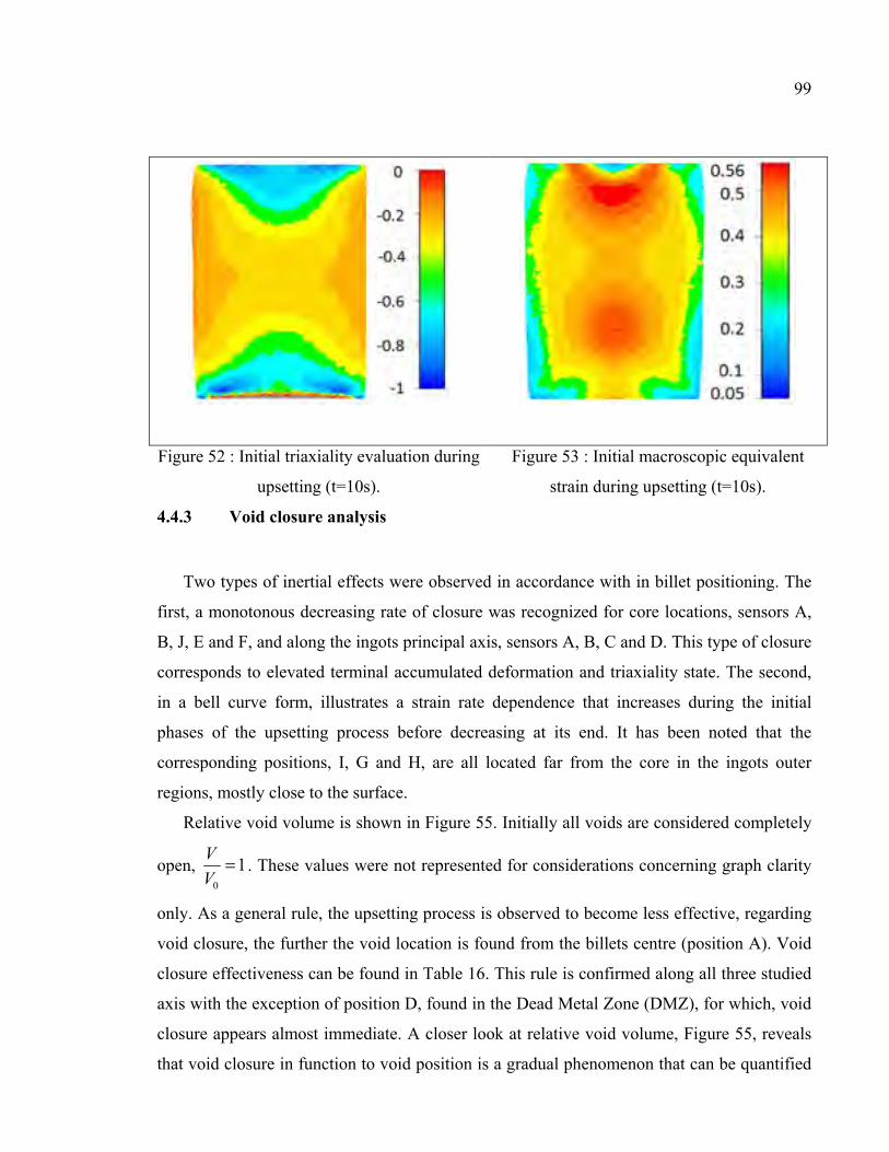
99
Figure 52 : Initial triaxiality evaluation during
upsetting (t=10s).
Figure 53 : Initial macroscopic equivalent
strain during upsetting (t=10s).
4.4.3 Void closure analysis
Two types of inertial effects were observed in accordance with in billet positioning. The
first, a monotonous decreasing rate of closure was recognized for core locations, sensors A,
B, J, E and F, and along the ingots principal axis, sensors A, B, C and D. This type of closure
corresponds to elevated terminal accumulated deformation and triaxiality state. The second,
in a bell curve form, illustrates a strain rate dependence that increases during the initial
phases of the upsetting process before decreasing at its end. It has been noted that the
corresponding positions, I, G and H, are all located far from the core in the ingots outer
regions, mostly close to the surface.
Relative void volume is shown in Figure 55. Initially all voids are considered completely
open, 0
1V
V= . These values were not represented for considerations concerning graph clarity
only. As a general rule, the upsetting process is observed to become less effective, regarding
void closure, the further the void location is found from the billets centre (position A). Void
closure effectiveness can be found in Table 16. This rule is confirmed along all three studied
axis with the exception of position D, found in the Dead Metal Zone (DMZ), for which, void
closure appears almost immediate. A closer look at relative void volume, Figure 55, reveals
that void closure in function to void position is a gradual phenomenon that can be quantified

100
by zone. Similar rates of void closure were observed for: positions A and E (the inner core)
and positions B, C, J and F (the outer core). Other zones, characterised in Table 15, all
showed unique results for void closure. The outer region, central outer region (position G)
and the upper outer region (position H), showed the least favourable conditions for void
closure. Out of these two, position H, displayed the least effective void closure for the
upsetting phase.
Combining the information from both Figure 54 and Figure 55 can better illustrate the
results. Figure 55 shows the void position D to be the most effective for void closure.
However, position D is also shown to appear in the billets DMZ figuring no material
displacement. Figure 54 reveals a near non-existent dependence (less than 5%) on strain at
this particular location during the entire upsetting phase. Position H shows the least gain in
void closure, Figure 55. This in-DMZ location exhibits low triaxiality states, 0.4xT < , but
not as little as in the central outer region, 0.3xT < . However, the relative void volume in
position G decreases quicker than in position H. Figure 55 helps clarify the phenomenon.
Position H has longer time related dependence on strain variation (larger bell curve), even
though maximum volumetric strain rate is similar. Void closure for H is therefore more
difficult because of it being more strain dependent for a longer period of time than in G.
Table 16 : Void closure effectiveness per axis
Axis Void Closure Effectiveness
Most Effective Least Effective
Vertical D A B C
Horizontal A E F G
45˚ inclined A J I H

101
Figure 54 : Accumulated equivalent
deformation dependence during ingot
upsetting.
Figure 55 : Relative void closure during the
upsetting process.
4.5 Conclusion
A methodology is proposed to evaluate void closure and observe corresponding forging
effects in an industrial size high strength steel ingot. Initial void positon (particularly central
regions) and relative strain dependence have significant effects on the void closure. Void
closure, although linearly gradual (axis Y and Z), can be observed by zone. The outer ingot,
especially upper outer ingot, must be targeted in order to optimize the forging process.
4.6 Acknowledgements
The authors wish to express their gratitude to Finkl Steel-Sorel Co. for providing the
equipment for the present research. The authors would like to appreciate NSERC for their
support in the framework of a Collaborative Research and Development project (CRD), and
Transvalor Americas Corp for permission to use Forge NxT 1.0® software. The authors
acknowledge access to high performance supercomputers at CLUMEQ.

102
4.7 References
[1] Dudra, S.P. and Y.-T. Im, Analysis of void closure in open-die forging. International Journal of Machine Tools and Manufacture, 1990. 30(1): p. 65-75.
[2] Lee, B.J. and M.E. Mear, Studies of the Growth and Collapse of Voids in Viscous Solids. Journal of Engineering Materials and Technology, 1994. 116(3): p. 348-358.
[3] Tkadlečková, M., K. Michalek, K. Gryc, B. Smetana, P. Machovčák, and L. Socha, The effect of boundary conditions of casting on the size of porosity of heavy steel ingot. Journal of Achievements in Materials and Manufacturing Engineering, 2013. 56(1): p. 9.
[4] Zhang, X.-X., Z.-S. Cui, W. Chen, and Y. Li, A criterion for void closure in large ingots during hot forging. Journal of Materials Processing Technology, 2009. 209(4): p. 1950-1959.
[5] Saby, M., P.O. Bouchard, and M. Bernacki, Void closure criteria for hot metal forming: A review. Journal of Manufacturing Processes, 2015. 19(0): p. 239-250.
[6] Lin, Y.C., M.-S. Chen, and J. Zhong, Numerical simulation for stress/strain distribution and microstructural evolution in 42CrMo steel during hot upsetting process. Computational Materials Science, 2008. 43(4): p. 1117-1122.
[7] Kakimoto, H., T. Arikawa, Y. Takahashi, T. Tanaka, and Y. Imaida, Development of forging process design to close internal voids. Journal of Materials Processing Technology, 2010. 210(3): p. 415-422.
[8] Lee, Y.S., S.U. Lee, C.J. Van Tyne, B.D. Joo, and Y.H. Moon, Internal void closure during the forging of large cast ingots using a simulation approach. Journal of Materials Processing Technology, 2011. 211(6): p. 1136-1145.
[9] Saby, M., M. Bernacki, E. Roux, and P.O. Bouchard, Three-dimensional analysis of real void closure at the meso-scale during hot metal forming processes. Computational Materials Science, 2013. 77(0): p. 194-201.
[10] FORGE NxT 1.0 ®, Transvalor S.A. : 694 av. Donat, 06255 Mougins Cedex, France. [11] Zhang, X.-X. and Z.-S. Cui, Theoretical study of void closure in nonlinear plastic
materials. Applied Mathematics and Mechanics, 2009. 30(5): p. 631-642. [12] P., H.Z. and W. J., Nonlinear Mechanics of Solids containing Isolated Voids Applied
Mechanics Review, 2006. 59: p. 20. [13] Chen, K., Y. Yang, G. Shao, and K. Liu, Strain function analysis method for void
closure in the forging process of the large-sized steel ingot. Computational Materials Science, 2012. 51(1): p. 72-77.
[14] Xu, B., M. Sun, and D. Li, Modeling of The Void Close Behavior in a 100t Ingot during Hot Forging. Metal Forming: p. 4.
[15] Zhang, X., F. Ma, K. Ma, and X. Li, Multi-scale Analysis of Void Closure for Heavy Ingot Hot Forging. Modern Applied Science, 2012. 6(10): p. 11.
[16] Saby, M., M. Bernacki, and P.-O. Bouchard, Understanding and Modeling of Void Closure Mechanisms in Hot Metal Forming Processes: A Multiscale Approach. Procedia Engineering, 2014. 81(0): p. 137-142.

103
[17] K.Chadha, D.Shahriari, and M.Jahazi, An Approach to Develop Hansel-Spittel Constitutive Equation during Ingot Breakdown Operation of Low Alloy Steels. FiMPART, 2015: p. 6.
[18] Kut, S., State of Stress Identification in numerical modeling of 3D issues. Archives of Metallurgy and Materials, 2009. 54(3).


CHAPTER 5
DEVELOPMENT OF A PREDICTION TOOL FOR SUCCESFUL FORGING
5.1 Forge Calculus – prediction tool
Forge Calculus is an in house code which was developed and continues development in the
framework of the current M.A.Sc. The program was written and is run using Matlab
2012.The code analyses .csv files exported directly from the position and force sensors used
at Sorel Forge.
Forge Calculus analyses forging data with a minimum of human input. A forging plan is
needed initially, see example p131, in order for a complete analysis to run. The code is
written to calculate and quantify indicators for each of the sequences described in 2.2.
Individual or global results can be visualised.
Global results include a statistical analysis of the forging database formed with the initial
data analysis code. Results show trends and standardisation measures for over 70 forged
parts. The amount of data analysed validates the significance of the averages calculated. The
quantification of indicator values and variability can then be used for comparison with real-
time forgings. These three functions are separated in order to increase program usability. The
main user interface can be seen in Figure 56.

106
Figure 56 : Forge Calculus main interface
5.1.1 In depth analysis of successful forgings
This section contains the models and algorithms used for studying each of the different
sequences in 2.2. The similarities observed in the forging process between upsetting and FM
respectively Cogging and Finishing are also reflected in the models conceived and the code
generated.

107
5.1.1.1 Sequence models
Upsetting and FM model
The first two sequences use the mathematical model in Figure 57 based on the following
premises:
• Contact is achieved between the workpiece and the factory floor.
• An intermediate die is needed during forging.
• The position sensor was successfully calibrated at the beginning of the working day.
(‘0’ occurs when the upper and lower dies touch).
Figure 57 : Upset and FM modeling diagram
The height of the ingot during forging is thus deduced as shown in (5.1).
_ int_ingot low die dieh pos h h= + −
(5.1)
Ingot width or height is given directly by posduring cogging and finishing because no
intermediate die is used and contact is therefore produced between upper die, workpiece and
the lower die.

108
A constant volume hypothesis is used in order to calculate ingot diameter and other initial
sequence indicators for upsetting and FM process. The loss of oxidised layers is accounted
for in a later calculation. Calculations for the upsetting sequence are derived from Figure 58
which shows both initial and final forms. 1h represents the height loss of the upset material.
Figure 58 : Upsetting initial and final states
The percentage of upset material is calculated as:
1
upseti
hr
h=
(5.2)
The reduction is deduced using:
1
i
i
hr
h h=
−
(5.3)
Reduction is verified according to the following formula and ingot height after upsetting
(5.1) :
1f ih h
r=
(5.4)
The final workpiece diameter is then calculated as:
.f id d r= (5.5)
An identical method is applied for FM sequence calculations.

109
Cogging and Finishing model
Cogging and Finishing models are based on Figure 59. Three stages are depicted; before bite,
after bite and before the consecutive bite. The third stage shows the manipulator having
advanced the workpiece of a certain feed length in order to continue forging.
Figure 59 : Cogging and finishing model
Bite depth and width (or Anvil Width Ratio – AWR) are calculated as
1 2h h hΔ = − (5.6)
3AWR
wr
h=
(5.7)
The half forging ratio indicates the time taken to forge half of the part in comparison to total
forging time.
hf
hftot
tr
t=
(5.8)

110
All sequence models
All equations in 5.1.1 are initially calculated as instantaneous values before using the
averages for individual forging indicator results, see 0. This allows the visualisation of
indicator evaluation during forging before consulting mean values. Upper die velocity, iv ,
and force ratio, iFr , are given as an example: For an instant i:
1 1
1 1
i i ii
i i i
h h hv
t t t+ −
+ −
Δ −= =Δ −
(5.9)
maxi
iF
Fr
F=
(5.10)
ihΔ and itΔ representing the variation in part height and the time taken respectively during
the instant i.
Averages are calculated using the arithmetic mean value:
1
1 n
ii
x xn =
= (5.11)
n being the amount of samples.
Material loss during forging
The forging plan, see APPENDIX I, p131, shows final measurements and weight for a forged
part. The length displayed corresponds to the length of useable material after machining. The
metal density per forging can therefore be deducted using (5.12) knowing the final shape is a
slab.
* *
weight
length height widthρ =
(5.12)
This formula assumes the metal density to be constant in the solidified steel slab.
Metal density is used to calculate initial volume before forging, knowing initial weight
(Appendix I, p131) and the volume percentage of the ingot hot top.
(1 )* _hottopi
perc initial weightV
ρ−
= (5.13)

111
Ingot geometry after finishing can be found in Appendix I, p131. A more precise calculation
for volume after forging is considered, accounting for the billet’s rounded edges using the
following hypothesis:
• The length of useable material after machining is equal to 1l
• The corners all have the same radius, r , after forging.
Figure 60 : Billet final volume schematic
Final width and height are read using Appendix I, p131, and verified using sensor data. The
final volume is calculated as:
1 2
1 1
2 1 2
1
2
2
2 1
2*
* *
( 2* )*
( 2* )*
4
fV V V
V l w h
V A A h
A w r r
rA
r l l
π
= +
== += −
=
= −
(5.14)
Process efficiency in terms of volume, or loss of volume, can be calculated with (5.15).
f
toti
V
Vη =
(5.15)
The weight of lost material can be quantified as can the associated cost using equations
(5.16) and (5.17).

112
_ (1 )* *tot iweight loss Vη ρ= − (5.16)
_ * _steel gradeworth weight lossκ= (5.17)
With _steel gradeκ the cost of the specific steel per kilo.
The efficiency of the finishing sequence can be assessed using the previous method with the
part volume after cogging, see Appendix I, p131.
_
ffinish
after cog
V
Vη =
(5.18)
Process efficiency can also be calculated for the first three sequences in the following
manner:
* * *tot i upset FM cog finishi
η η η η η η= =∏ with 1 3 * *seq upset FM cogη η η η− = (5.19)
1 3
totseq
finish
ηηη− =
(5.20)
5.1.1.2 Sequence algorithms
The main algorithms used in Forge Calculus are detailed in this paragraph. A simplified code
is presented for a better understanding of the software’s logic. The accuracy of the results
obtained from the previous models depends on sensor precision, namely the sampling
frequency and discretisation. Elimination of unwanted movements or noise was also an
important task.
Terminology:
DB: Database
Underlined word: Major sub-routine that will be explained
Bold word: Important step in the program

113
Main
Program description: The main is used to run Forge Calculus and all sub-routines when they
are asked to. The information is read, analysed and the results displayed using an intuitive
user interface.
Simplified code:
Initialisation Generate Main User Interface Create new /Load existing DB Collect Information if asked Read sensor .csv files
Determine if the file is new/ the next part of an existing file/ or has already been analysed. If file=new Then Create new entry in DB using a standardised template Data Analysis Fill the template If file=next part of an existing file Then Load existing file template Data Analysis Fill existing file template End If Save DB
Analyse DB if asked (see Appendix II, p133, for DB structure at this point) Sort DB into Sequences Create new Sequence DB’s Save Sequence DB’s If Individual results selected Then Display selected data Else if Global results selected Then Run Statistical Analysis for selected indicator Show Results End If End of Main
Data Analysis
Program description: This sub-routine is the bedrock for the Forge Calculus. All future
analysis for individual and global results depends on the values calculated in Data Analysis.
The data file is separated into several parts equivalent to different identified sequences. An
essential part of each sequence is determining the moment when contact is established

114
between the upper die and the workpiece (local force condition) and the moment when the
contact is broken (local position condition). As previously explained, upsetting and the FM
process respectively cogging and finishing both have similar source code. The mathematical
formulae can be found in 5.1.1.1.
Simplified code:
Determine which sequence is currently under analysis If sequence = Upsetting Then load initial geometry for specific casting number Identify specific sequence time delimiters, t1 and t2 For t1 to t2 Calculate start and finish stroke times, ti End for Calculate the variations in position, speed and force for the ti Calculate Upsetting indicators (5.1.1.1) Calculate Geometry and weight after upsetting Else if sequence = FM Then load end of upset geometry for specific casting number Identify specific sequence time delimiters, t1 and t2 For t1 to t2 Calculate start and finish stroke times, ti End for
Calculate the variations in position, speed and force for the ti Calculate FM indicators (5.1.1.1) Calculate Geometry and weight after FM Else if sequence = Cogging Then load end of FM geometry
Calculate the time delimiters, t1 to tn, that correspond to a 90 rotation of the workpiece Assign work on ‘width’ or ‘height’ to corresponding delimiters i=1 While i<=n For t=ti to t=ti+1
Calculate time delimiters, tt2 to ttm, that correspond to start of pass (reversal in travelling) j=1 While j<=m For t=ttj to ttj+1
Calculate start and finish stroke times, ttti
Calculate the variation in position, speed and force for the ttti Calculate Cogging Indicators End For

115
j=j+1 End While End For i=i+1
End While Calculate cogging geometry Else If sequence = Finishing Then load end of cogging geometry
Calculate the time delimiters, t1 to tn, that correspond to a 90 rotation of the workpiece Assign work on ‘width’ or ‘height’ to corresponding delimiters i=1 While i<=n For t=ti to t=ti+1
Calculate time delimiters, tt2 to ttm, that correspond to start of pass (reversal in travelling) j=1 While j<=m For t=ttj to ttj+1
Calculate start and finish stroke times, ttti
Calculate the variation in position, speed and force for the ttti Calculate Finishing Indicators End For
j=j+1 End While End For i=i+1
End While Calculate finishing geometry End If End of Data Analysis Statistical Analysis
Program description: The statistical analysis program analyses the individual sequence
databases created in Main. Twenty probability density models, see Appendix III, p135, are
available for comparison. The selected indicator distribution is analysed using relevant
density functions and the results are classed. The most suitable model is integrated between
limits set by the user to calculate event probability.

116
Simplified code
Create a simplified histogram For i=1 to the number of distributions to compare If the data meets model requirements Then Calculate probability density function Calculate comparison indexes: NLogL, BIC, AIC, AICc End If Compare results and sort list Create a more detailed histogram Add three best comparisons Integrate most suitable function if probability calculation is required End of Statistical Analysis 5.1.1.3 Example of application
The following section shows application of the previous code to one forged part. This
particular file was chosen because of the high frequency of measure and precision entailed in
the ensuing calculations. The data for the forged part is split into two files. The first
regarding the Upsetting, FM and Cogging processes. The second concerns the Finishing
process. Both files contain between 20000 and 25000 lines of data to be analysed each
representing two hours of data recording. Part temperature was homogenised in a furnace
during the two recordings in order to obtain better workability for the finishing sequence.
Forging Charts
The forging chart (hydraulic press position – blue, and Forging Force – green) for Files 1 and
2 can be seen in Figure 61 and Figure 62. The global index on the x axis corresponds to the
number of the line of data. In this case the data from 15000 to 22000 was removed because
the forging had already completed. The different sequences of Upset (1), FM (2) and
Cogging (3) have been outlined in order to cross reference the following analysis with the
Forging chart, Figure 61. The whole of the Figure 62 is the second and final forging for this
part, also known as Finishing.

117
Figure 61: Forging chart – First forging, 1: Upsetting, 2: FM, 3: Cogging
Figure 62 : Forging chart - Second forging, Finishing
Two conditions are necessary in order to successfully calculate stroke times, a crucial step in
the forging data analysis algorithm. The first is the need for a sufficient forging force. The
second, that material deformation only occurs when the upper anvil draws nearer to the lower
anvil. These two conditions can be modelled through equations and algorithms. The force
condition is predominant and as such is the first filter used in this analysis. The force filter
results are then used as input for the position filter or second condition.

118
The force filter can be seen for The Upsetting and FM sequences respectively in Figure 63
and Figure 64. The forging force is represented alongside local minima (black circles) and
local maxima (red circles) in each graph. The upper graph shows unfiltered results which
contain several parasitic values due to sensor precision. The first stage of the force filter, seen
in the middle graph, cleans and calculates alternating data minima and maxima. The second
stage, the lower graph, delimits each force peak either side. The two delimiting values and
the maximum of each force peak are inputs for the position filter.
Notice that even though the Upset and FM processes are theoretically one stroke sequences
several anvil blows can be observed, five blows being used for this particular forging. This is
because the maximal forging force of 5000T has been reached and the ingot to forge is too
massive for brute force alone. A slight momentum is given to the upper anvil in order to
compensate this lack.
Figure 63 : Upset sequence, Force filter

119
Figure 64 : FM sequence, Force filter
The position filter analyses a triplet of global indexes [force peak start, force peak maximum,
force peak stop] for each force peak previously recognised. The values are transferred to the
press position curve. A search for start hit press position is accomplished for values between
force peak start index and force peak maximum index. A search for stop hit press position is
then carried out for values from force peak maximum to force peak stop. Criteria for a
successful search include a sufficient forging force (equivalent to forging values superior to a
threshold which is a percentage of the current force peaks maximal value) and a decreasing
position curve. Part reduction curves for the Upset and FM process of this forging can be
seen respectively in Figure 65 and Figure 66. The start and stop hits for each force peak are
represented by the red and black circles.
Figure 65 : Upset sequence, Part reduction

120
Figure 66 : FM sequence, Part reduction
The calculation of process indicators is then simply the application of the equations from
5.1.1.1. Table 17 and Table 18 show results for both sequences per hit of the anvil. Press
speed is initially high (30-40 mm.s-1) before rapidly decreasing as the anvil loses momentum
and the forged material becomes more compressed. The Upset sequence shows higher press
velocity values than that of the FM sequence. This shows that the material effects created
during Upsetting must be overcome during FM. Table 19 shows average results for both
sequences. These results are less representative of the process because the sampling period is
larger, but the results are useful for simple process characterisation and can be applied in FE
process simulations.
Results per hit
Table 17 : Upset results per hit of anvil
UPSET Start time (s) Stop time (s) Amount Upset (mm) Press velocity (mm.s-1)
hit 1 189.6 206.2 738.12 44.65
hit 2 207.4 217.4 148.08 14.80
hit 3 222.2 255.2 580.89 17.60
hit 4 256.4 287.4 381 12.29
hit 5 288.6 322.6 300.22 8.8

121
Table 18 : FM results per hit of anvil
FM Start time (s) Stop time (s) Amount Upset (mm) Press velocity (mm.s-1)
hit 1 936.2 953 560.83 33.38
hit 2 654.6 977.8 227.58 9.81
hit 3 979.2 1008 150.11 4.8
hit 4 1022 1031 142.24 4.81
hit 5 1033 1077 158.49 3.55
Average results
Table 19 : Average Upset and FM indicators
Process time (s)
Amount
Upset (mm)
Average velocity
(mm.s-1) Reduction
Percentage of
Upset
Upset 125 2148 17.2 2 49.7
FM 135 1239 9.1 1.12 57.3
The real difficulty of this analysis is the flexibility of the code, especially concerning the
filters. The same or very similar filters are used for the cogging and finishing sequences even
though the data and consequential curves are a very different form. The code must also be
able to cope with unexpected operator movements during forging. Each forging is completed
with over 95% being manual, each operator reacting differently to the state of the ingot based
on his past experience and what he sees in front of him. Patterns are therefore a lot more
subtle to recognise when coding.
The approach to analysing the Cogging and Finishing sequences follows a logic that aims to
apply the same methods and algorithms used in the Upset and FM analysis. The data range is
split into shorter working sequences in order to increase the precision of results. Definition of
work sequences are shown in Figure 67 and Figure 68. The algorithm determines an indicator
based on press position which shows each time the manipulator rotates 90 degrees with part
in hand. Therefore separating forging mainly part width (above indicator) and mainly part
height (below indicator). As previously specified in 2.4.2, the press position curves for

122
Cogging and Finishing display significantly different aspects due to part shape at time of
forging.
Figure 67 : Cogging - Work sequence definition
Figure 68 : Finishing - Work sequence definition
As well as rotating 90 degrees around its principal axis in between working on part height
and width, the part also travels to and from the anvils in order to complete successive blows
during the Cogging and Finishing sequences. A pass is defined as a significant change in part

123
travel direction. Passes can include a variable amount of work or blows from the press
depending on forging progression. The number of hits increases with forging progression and
part length. Each work sequence can contain a variable amount of passes as shown by Figure
69 and Figure 70. A decrease and increase respectively in travelling value means that the
manipulator grabbing hand and the part are advancing respectively towards and away from
the press anvil. A Work sequences are observed to incorporate more passes during Finishing
in relation to Cogging. A greater number of force peaks per pass are counted during
Finishing. However the deformation per hit is reduced. A pass is considered insignificant if it
is defined without corresponding force peaks.
Figure 69 : Cogging - Work sequence 19 - Travel analysis

124
Figure 70 : Finishing - Work sequence 10 - Travel analysis
On top of back and forward movement, rotation around the parts principal axis and working
on part height and width, the part undergoes one 180 degree rotation around a vertical axis
with the help of the bridge crane. This rotation is equivalent to a half forging completion and
marks the start of forging on the second half of the ingot. Figure 71 shows half forging
completion detection for Cogging. The data point is also a point of theoretical symmetry
which is particularly visible in the press position curve, see Figure 67 , with the same global
index position. The symmetry is present in the numerical values of several calculated
indicators.
Figure 71 : Cogging - Half forging completion

125
After analysing travelling data, the force peaks for each work sequence are identified
identically to the method used during Upsetting and the FM sequence. The position filter is
also used to calculate all relative sequence indicators as proposed in 5.1.1.1. Figure 72 shows
part reduction calculation for Finishing, work sequence 10. Staircase forging, as explained in
2.4.2, is observed. In this example, 6 one way passes are performed before completing a
series of two way passes, starting in the zoom of Figure 72. The movement of the
manipulator for the one way passes is a withdrawal from the press or backward. This means
that the flow of material during deformation is from the end held by the manipulator towards
the ingots free end. The part is essentially being stretched out, with material feeding the free
end. This material flow pattern is characteristic of a successful forging technique. The
deformation and deformation rate is shown to be greater for one way passes. The second pass
of the two way passes, forward, is therefore a lot less significant for successful forging and is
used just for part geometry homogeneity.
Figure 72 : Finishing - Work sequence 10 - Part reduction with zoom
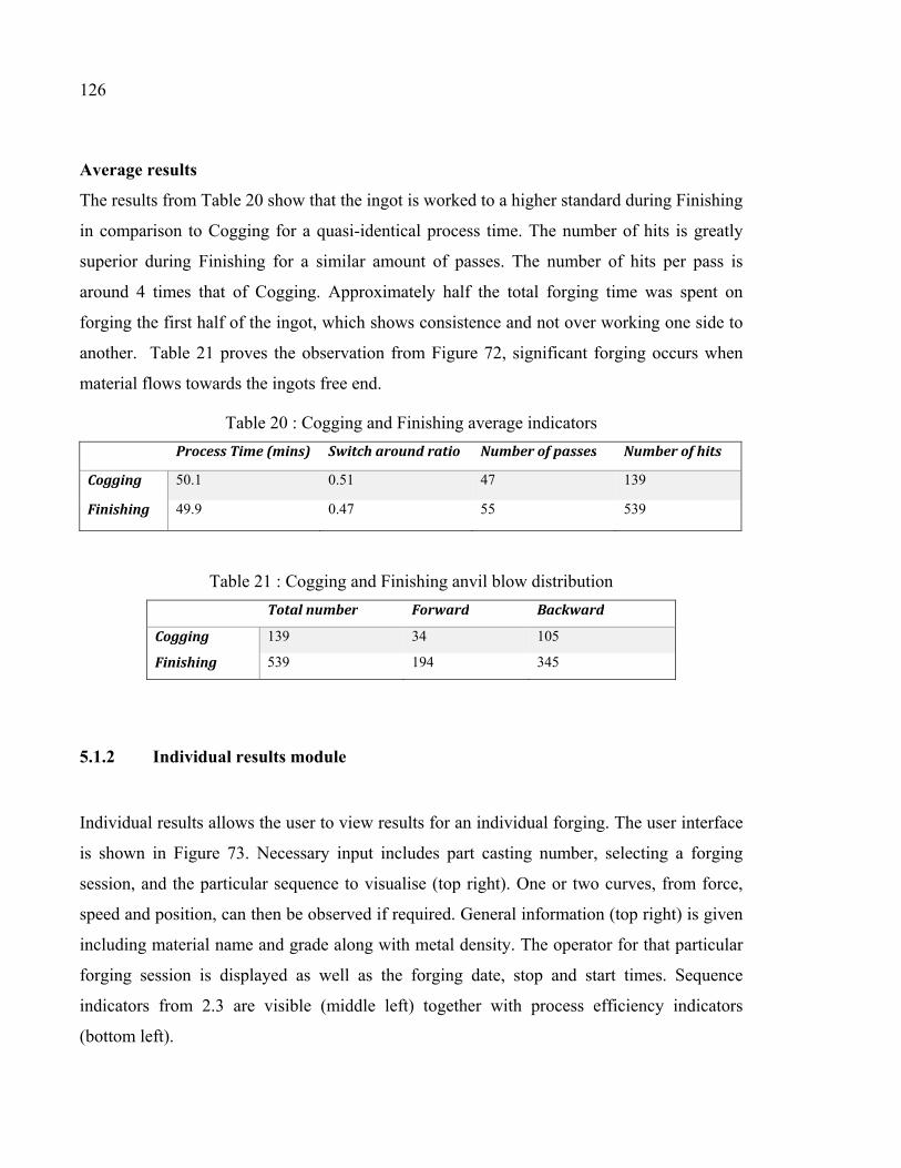
126
Average results
The results from Table 20 show that the ingot is worked to a higher standard during Finishing
in comparison to Cogging for a quasi-identical process time. The number of hits is greatly
superior during Finishing for a similar amount of passes. The number of hits per pass is
around 4 times that of Cogging. Approximately half the total forging time was spent on
forging the first half of the ingot, which shows consistence and not over working one side to
another. Table 21 proves the observation from Figure 72, significant forging occurs when
material flows towards the ingots free end.
Table 20 : Cogging and Finishing average indicators
Process Time (mins) Switch around ratio Number of passes Number of hits
Cogging 50.1 0.51 47 139
Finishing 49.9 0.47 55 539
Table 21 : Cogging and Finishing anvil blow distribution
Total number Forward Backward
Cogging 139 34 105
Finishing 539 194 345
5.1.2 Individual results module
Individual results allows the user to view results for an individual forging. The user interface
is shown in Figure 73. Necessary input includes part casting number, selecting a forging
session, and the particular sequence to visualise (top right). One or two curves, from force,
speed and position, can then be observed if required. General information (top right) is given
including material name and grade along with metal density. The operator for that particular
forging session is displayed as well as the forging date, stop and start times. Sequence
indicators from 2.3 are visible (middle left) together with process efficiency indicators
(bottom left).

127
Potential use for this function would be for part inspection if the part was found not to
conform to client specifications. A retroactive control could then take place for fault finding,
taking a closer look at each forging sequence.
Figure 73 : Individual results user interface
5.1.3 Statistical analysis module
Global results combines information from each individual part forging and sorts the result by
sequence. The user interface can be seen in Figure 74, with input being sequence and
indicator selection (top left). A simplified histogram (left hand graph) and a more detailed
distribution (right hand graph) of the empirical data is displayed. Probability density function
matches are superimposed on the latter to show correlation. Parameters for the most suitable
function are given. Sample size and standard indicator values (bottom left) are displayed to
characterize the forging process. A probability calculation is available if the user wishes to
calculate the occurrence of a particular event.

128
This function gives base line values for future forgings. The indicator standards characterize
successful forgings and can therefore be useful for future successful forging predictions.
Figure 74 : Global results user interface
5.2 Future development
A tool able to analyse and characterize forged part sequences is only the beginning. This tool
should be used as a platform for future development. A study validating the relevance of the
chosen indicators and their standard values in relation to successful forgings should be
completed.
A second study, looking at the interdependence between the relative sequence indicators,
would then begin the development of a function capable of predicting the probability of a
successful forging. Validation of this function could be simulated, emulating forgings
conditions for each indicator.
The final action would be the implication of the developed prediction function into the
company itself. The emulation of forging conditions would be replaced with a live data feed
directly from the sensors in the forge. The information would be treated live and the
probability function would show the operator if he was statistically following the guidelines
set by a database of successful forgings.

CONCLUSIONS
A fast converging material specific void closure model was developed in order to assess void
closure for explicit high strength steels from the industrial partner. The coupled effect of
increased triaxiality states and Norton exponents was shown to have a positive effect on void
closure potential. The model was then used in a full field FEM simulation, Forge Nxt 1.0 ®,
for an open die forging sequence of a 40T ingot. The upsetting sequence was selected
because it represents the first significant sequence of hot deformation and therefore greatly
impacts upon void closure. Core areas in the ingot displayed the highest void closure
potential followed by the outer core and a central zone close to the upper die. Peripheral
regions showed the least potential, proving the necessity and effectiveness of the FM process.
Large amounts of experimental data from the industrial partner regarding slab forging were
generated and analysed with an in-house code using Matlab 2012. The forging of over 70
parts was characterised individually and then globally using a statistical analysis. The results
include standardised indicators for successful forgings and a possible future quality control.
Forge Calculus, new software for predicting successful open die high strength steel slab
forgings from large ingots was developed in order to optimise forging conditions for void
elimination.
The framework was defined according to an in depth study of industrial steel grades, forging
processes and existing void closure models. Application of the latter to industrial case
forgings was found to be missing in current literature. The open die forging process was
found to incorporate five forging sequences including initial forming of a square base,
upsetting, FM process, cogging and finishing. Initial forming was proven to be insignificant
in terms of applied deformation and residual stress in ingot. Similarity in deformation effects
on workpiece topology was observed for both the upsetting and FM respectively cogging and
finishing sequences. The similarities detected are also noticeable in Forge Calculus data
analysis code.

130
An intuitive user interface was designed in order to facilitate the visualisation and accelerate
certain calculations. Real time forging quality predictions are discussed as an interesting
future development for Forge Calculus.

APPENDIX I
Forging plan example


APPENDIX II
Main Database Structure


APPENDIX III
Probability function list
Distribution Type Formula : y= Probability density function Information
Beta 1 1(0,1)
1( | , ) (1 ) ( )
( , )a by f x a b x x I x
B a b− −= = − B( · ) is the Beta
function
Binomial ( | , ) (1 )k n kn
y f k n p p pk
− = = −
Birnbaum-
Saunders
2
2
1exp
2 22
x xx x
yx
β ββ β
γ γπ
− + = −
β > 0 , γ >0 x > 0
Burr Type XII 1( | , , ) 1
1
kcy F x c k
xα
α
= = − +
0, 0, 0, 0x c kα> > > >
Exponential 1( | )
x
y f x e μμμ
−
= =
Extreme value 1( | , ) exp exp exp
x xy f x
μ μμ σσ σ σ
− − = = −
Gamma ( ) 11
| ,( )
xa b
ay f x a b x e
b a
−−= =
Γ
Γ( · ) is the Gamma
function
Generalised
extreme value
1 1(1 )
1( | , , ) exp 1 1
k kx xy f x k k k
μ μμ σσ σ σ
− − + − − = = − + +
Generalised
Pareto
1(1 )
1( | , , ) 1
kxy f x k k
θσ θσ σ
− +− = = +
θ < x, k >0, or θ < x
<–σ/k for k <0

136
Inverse Gaussian 2
3 2exp ( )
2 2y x
x x
λ λ μπ μ
= − −
Logistic
2
1
x
x
ey
e
μσ
μσσ
−
−=
+
Log-logistic ln( )
2ln( )
1
x
x
ey
e
μσ
μσσ
−
−=
+
Lognormal 2
2
(ln )
21( | , )
2
x
y f x ex
μσμ σ
σ π
− −
= =
Nakagami 2(2 1)1
2( )
xy x e
μ μμ ωμ
ω μ
−− = Γ
ω > 0 for x > 0
Normal 2
2
( )
21( | , )
2
x
y f x eμ
σμ σσ π
− −
= =
Poisson (0,1,..)( | ) ( )
!
x
y f x e I xx
λλλ −= =
Rayleigh 2
222
( | )x
bx
y f x b eb
−
= =
Rician 2 2
220 2 2
x sxs x
y I e σ
σ σ
+− =
s ≥ 0, σ > 0, for x >0.
I0 is the zero order
Bessel function.
t Location - Scale 12 21
2
2
x
y
υ
υ μυσ
υ υσ υπ
+ − + − Γ +
= Γ
σ >0, ν > 0
Weibull 1
( | , )
bb x
ab xy f x a b e
a a
− − = =
x>0, a>0, b>0,

BIBLIOGRAPHY
(FORGE NxT 1.0 ®). 694 av. Donat, 06255 Mougins Cedex, France, Transvalor S.A. . Azushima, A., et al. (2012). "Coefficient of friction at interface of lubricated upsetting
process." Wear 286–287(0): 3-7. Banaszek, G. and A. Stefanik (2006). "Theoretical and laboratory modelling of the closure of
metallurgical defects during forming of a forging." Journal of Materials Processing Technology 177(1–3): 238-242.
Budiansky, B., et al. (1982). "Void growth and collapse in viscous solids." Pergamon Press,
Oxford: 32. Carroll, J. D., et al. (2012). "The effect of grain size on local deformation near a void-like
stress concentration." International Journal of Plasticity 39(0): 46-60. Chen, D.-C. (2006). "Rigid-plastic finite element analysis of plastic deformation of porous
metal sheets containing internal void defects." Journal of Materials Processing Technology 180(1–3): 193-200.
Chen, K., et al. (2012). "Strain function analysis method for void closure in the forging
process of the large-sized steel ingot." Computational Materials Science 51(1): 72-77. Chen, M.-S. and Y. C. Lin (2013). "Numerical simulation and experimental verification of
void evolution inside large forgings during hot working." International Journal of Plasticity 49(0): 53-70.
Chen, M.-S., et al. (2014). "Evolution of elliptic-cylindrical and circular-cylindrical voids
inside power-law viscous solids." International Journal of Plasticity 53(0): 206-227. Cho, J. R., et al. (1998). "Analysis of the cogging process for heavy ingots by finite element
method and physical modelling method." Journal of Materials Processing Technology 80–81(0): 161-165.
Dudra, S. P. and Y.-T. Im (1990). "Analysis of void closure in open-die forging."
International Journal of Machine Tools and Manufacture 30(1): 65-75. Duva, J. M. and J. W. Hutchinson (1984). "Constitutive potentials for dilutely voided
nonlinear materials." Mechanics of Materials 3(1): 41-54. Everett, R. K., et al. (2001). "Spatial distribution of voids in HY-100 steel by X-ray
tomography." Scripta Materialia 44(1): 165-169.

138
Fleck, N. A. and J. W. Hutchinson (2001). "A reformulation of strain gradient plasticity." Journal of the Mechanics and Physics of Solids 49(10): 2245-2271.
Gurson, A. L. (1977). "Continuum Theory of Ductile Rupture by Void Nucleation and
Growth: Part I—Yield Criteria and Flow Rules for Porous Ductile Media." Journal of Engineering Materials and Technology 99(1): 2-15.
He, M. Y. and J. W. Hutchinson (1981). "The Penny-Shaped Crack and the Plane Strain
Crack in an Infinite Body of Power-Law Material." Journal of Applied Mechanics 48(4): 830-840.
Huang., Z. P. and J. Wang. (2006). "Nonlinear Mechanics of Solids containing Isolated
Voids " Applied Mechanics Review 59: 20. K.Chadha, et al. (2015). "An Approach to Develop Hansel-Spittel Constitutive Equation
during Ingot Breakdown Operation of Low Alloy Steels." FiMPART: 6. Kakimoto, H., et al. (2010). "Development of forging process design to close internal voids."
Journal of Materials Processing Technology 210(3): 415-422. Keife, H. and U. Ståhlberg (1980). "Influence of pressure on the closure of voids during
plastic deformation." Journal of Mechanical Working Technology 4(2): 133-143. Kim, Y., et al. (2011). "Efficient forging process to improve the closing effect of the inner
void on an ultra-large ingot." Journal of Materials Processing Technology 211(6): 1005-1013.
Kut, S. (2009). "State of Stress Identification in numerical modeling of 3D issues." Archives
of Metallurgy and Materials 54(3). Lecarme, L., et al. (2014). "Heterogenous void growth revealed by in situ 3-D X-ray
microtomography using automatic cavity tracking." Acta Materialia 63: 130-139. Lee, B. J. and M. E. Mear (1994). "Studies of the Growth and Collapse of Voids in Viscous
Solids." Journal of Engineering Materials and Technology 116(3): 348-358. Lee, B. J. and M. E. Mear (1999). "Evolution of elliptical voids in power-law viscous solids."
Mechanics of Materials 31(1): 9-28. Lee, Y. S., et al. (2011). "Internal void closure during the forging of large cast ingots using a
simulation approach." Journal of Materials Processing Technology 211(6): 1136-1145.

139
Li, J., et al. (2014). "Simulation of macrosegregation in a 2.45-ton steel ingot using a three-phase mixed columnar-equiaxed model." International Journal of Heat and Mass Transfer 72: 668-679.
Lin, Y. C., et al. (2008). "Numerical simulation for stress/strain distribution and
microstructural evolution in 42CrMo steel during hot upsetting process." Computational Materials Science 43(4): 1117-1122.
Maire, E., et al. (2001). "On the Application of X-ray Microtomography in the Field of
Materials Science." Advanced Engineering Materials 3(8): 539-546. Montheillet, F. and J. J. Jonas (1996). "Temperature dependence of the rate sensitivity and its
effect on the activation energy." Metallurgical and Materials Transactions 27(10): 3. Niordson, C. F. (2008). "Void growth to coalescence in a non-local material." European
Journal of Mechanics - A/Solids 27(2): 222-233. P. M.Dixit, U. S. D. (2008). Modelling of Metal Forming and Machining Processes: by Finite
Element and Soft Computing Methods, Engineering Materials and Processes. Park, C. Y. and D. Y. Yang (1996). "A study of void crushing in large forgings I: Bonding
mechanism and estimation model for bonding efficiency." Journal of Materials Processing Technology 57(1–2): 129-140.
Ragab, A. R. (2004). "Application of an extended void growth model with strain hardening
and void shape evolution to ductile fracture under axisymmetric tension." Engineering Fracture Mechanics 71(11): 1515-1534.
Rice, J. R. and D. M. Tracey (1969). "On the ductile enlargement of voids in triaxial stress
fields∗." Journal of the Mechanics and Physics of Solids 17(3): 201-217. Roux, E., et al. (2013). "A level-set and anisotropic adaptive remeshing strategy for the
modeling of void growth under large plastic strain." Computational Materials Science 68(0): 32-46.
Saby, M. (2013). "Compréhension et modélisation des mécanismes de refermeture de
porosité dans les procédés de mise en forme des métaux à chaud." 234. Saby, M., et al. (2014). "Understanding and Modeling of Void Closure Mechanisms in Hot
Metal Forming Processes: A Multiscale Approach." Procedia Engineering 81(0): 137-142.
Saby, M., et al. (2013). "Analyse multi-échelle de la refermeture de porosités, appliquée à la
mise en forme des métaux à chaud." 11e Colloque National en Calcul des Structures.

140
Saby, M., et al. (2013). "Three-dimensional analysis of real void closure at the meso-scale during hot metal forming processes." Computational Materials Science 77(0): 194-201.
Saby, M., et al. (2015). "Void closure criteria for hot metal forming: A review." Journal of
Manufacturing Processes 19(0): 239-250. Samei, J., et al. (2016). "Influence of strain path on nucleation and growth of voids in dual
phase steel sheets." Materials & Design 92: 1028-1037. Song, M., et al. (2014). "In situ electron microscopy investigation of void healing in an Al–
Mg–Er alloy at a low temperature." Acta Materialia 69(0): 236-245. Sternberg, S. R. (1983). "Biomedical Image Processing." Computer 16(1): 22-34. Szelążek, J., et al. (2009). "New samples with artificial voids for ultrasonic investigation of
material damage due to creep." NDT & E International 42(2): 150-156. Tkadlečková, M., et al. (2013). "The effect of boundary conditions of casting on the size of
porosity of heavy steel ingot." Journal of Achievements in Materials and Manufacturing Engineering 56(1): 9.
Toda, H., et al. (2009). "Healing behavior of preexisting hydrogen micropores in aluminum
alloys during plastic deformation." Acta Materialia 57(15): 4391-4403. Tvergaard, V. (1982). "On localization in ductile materials containing spherical voids."
International Journal of Fracture 18(4): 237-252. Tvergaard, V. (1984). "On the creep constrained diffusive cavitation of grain boundary
facets." Journal of the Mechanics and Physics of Solids 32(5): 373-393. Xu, B., et al. "Modeling of The Void Close Behavior in a 100t Ingot during Hot Forging."
Metal Forming: 4. Zhang, J. (2016). 11 - Defect detection, classification, and characterization using ultrasound
A2 - Yuan, Fuh-Gwo. Structural Health Monitoring (SHM) in Aerospace Structures, Woodhead Publishing: 307-323.
Zhang, X.-X. and Z.-S. Cui (2009). "Theoretical study of void closure in nonlinear plastic
materials." Applied Mathematics and Mechanics 30(5): 631-642. Zhang, X.-X., et al. (2009). "A criterion for void closure in large ingots during hot forging."
Journal of Materials Processing Technology 209(4): 1950-1959.

141
Zhang, X., et al. (2012). "Multi-scale Analysis of Void Closure for Heavy Ingot Hot Forging." Modern Applied Science 6(10): 11.
Zhongxiao, J. and G. W. Stewart. (2000). "An analysis of the rayleigh-ritz method for
approximating eigenspaces." Mathematics of computation 70(234): 10.