Sponsor TBD Report No.:

AISI/DOE Technology Roadmap Program

Final Report

CHARACTERIZATION OF FATIGUE AND CRASH PERFORMANCE OF NEW GENERATION HIGH STRENGTH STEELS FOR AUTOMOTIVE

APPLICATIONS

By

Benda Yan, Principal Investigator Dennis Urban, Program Manager

April 2003

Work Performed under Cooperative Agreement No. DE-FC07-97ID13554

Prepared for

U.S. Department of Energy

Prepared by American Iron and Steel Institute

Technology Roadmap Program Office Pittsburgh, PA 15222

ii

DISCLAIMER

“Any opinions, findings, and conclusions or recommendations expressed in this material are those of the author(s) and do not necessarily reflect the views of the US Department of Energy.” Number of pages in this report: 97 For availability of this report, contact:

Office of Scientific and Technical Information P.O. Box 62 Oak Ridge, TN 37831 (615) 576-8401.

iii

TABLE OF CONTENTS

Page Table of Contents…………………………………………………………………………… iii List of Figures……………………………………………………………………………… iv List of Tables………………………………………………………………………………. v Executive Summary ……………………………………………………………………….. vi Acknowledgment……………………………………………………………………………..viii 1. Introduction………………………………………………………………………… 1 2. Steels …..………………………………………………………………………… 2 3. Fatigue Behavior…………………………………………………………………… 4 3.1 Experiments………………………………………………………………… 4

3.2 Results……………………………………………………………………… 4 3.2.1 Strain-controlled fatigue……………………………………………… 4 3.2.2 Fatigue of notched specimens………………………………………… 9

4. High Strain Rate Behavior…………………………………………………………. 12 4.1 Experiment……………………………………………………………………… 12 4.2 Results ………….. ……………………………………………………………. 15

4.2.1 Stress-strain data at high strain rates………………………………… ….. 15 4.2.2 YS and UTS ………………………………………………………………. 20 4.2.3 Elongation ………………………………………………………………… 20 4.2.4 n-value ……………………………………………………………………. 20 4.2.5 Energy absorption ………………………………………………………… 20

5. Conclusions………………………………………………………………………… 30 6. References………………………………………………………………………….. 31 7. Appendix: Phase 1 Report ……………………………………………… 32

iv

LIST OF FIGURES Figure 1 Engineering stress-strain curves for four steels in Phase 2 ………………… 4 Figure 2 Neuber stress vs. fatigue life curves for steels in Group 2 with minimum UTS of 590 – 600 MPa ……………………………………….… 6 Figure 3 Neuber stress vs. fatigue life curves for DP800-GA and TRIP780-CR …….. 6 Figure 4 Neuber stress vs. fatigue life curves for TRIP steels of different strength …. 7 Figure 5 ∆S/2 vs. fatigue life curves for steels in Group 2 with minimum UTS of 590 to 600 MPa …………………………………………… .……… 10 Figure 6 ∆S/2 vs. fatigue life curves for steels in Group 3, DP800-GA and TRIP780-CR ……………………………………………….. 11 Figure 7 ∆S/2 vs. fatigue life curves for TRIP steels of different strengths ……. ……. 11 Figure 8 Schematic of tensile specimen used for servo-hydraulic system with a strain gage at grip section …………………………….…………… 13 Figure 9 Comparison of stress-strain data at 100/s, using load cell vs. strain gage to measure load ……………………………………………………………. 14 Figure 10 Comparison of stress-strain data at 500/s, using load cell, strain gage and SHB, respectively …………………………………………. 14 Figure 11 Smoothed stress-strain curves for DP600-HR at various strain rates ……. 16 Figure 12 Smoothed stress-strain curves for TRIP600-CR at various strain rates ……. 16 Figure 13 Smoothed stress-strain curves for TRIP780-CR at various strain rates ……. 17 Figure 14 Smoothed stress-strain curves for TRIP980-CR at various strain rates ……. 17 Figure 15a Yield strength vs. strain rate for Dual Phase steels ………………………… 23 Figure 15b Yield strength vs. strain rate for TRIP steels ……………………………… 23 Figure 16a Ultimate tensile strength vs. strain rate for Dual Phase steels ……………… 24 Figure 16b Ultimate tensile strength vs. strain rate for TRIP steels …………………… 24 Figure 17 Increase in UTS per order of magnitude increase of strain rate vs. quasi-static UTS ………………………………………………………… 25 Figure 18a Uniform elongation vs. strain rate for Dual Phase steels …………………… 25 Figure 18b Uniform elongation vs. strain rate for TRIP steels ………………………… 26 Figure 19a Total elongation vs. strain rate for Dual Phase steels ………………………. 26 Figure 19b Total elongation vs. strain rate for TRIP steels ………… …………………. 27 Figure 20 n-value vs. strain rate for Dual Phase and TRIP steels ……………………… 27 Figure 21 Energy absorption before necking per unit volume, Enecking, vs. strain rate..… 28 Figure 22 Energy absorption below 10% strain, E10% , vs. strain rate………………… 28 Figure 23 Relationship between E10% and quasi-static UTS ……………..…………… 29 Figure 24 Increase in E10% per order of magnitude increase of strain rate vs. quasi-static UTS…………………………………………………………. 29

v

LIST OF TABLES Table 1 Tensile Properties …………………………………………………………… 3 Table 2 Fatigue Properties…………………………………………………………… 8 Table 3 True Flow Stresses at Various Strains Rates…………….………………….. 18 Table 4 Tensile Properties at Various Strain Rates………………………………….. 19 Table 5 Increase in UTS per Order of Magnitude Increase in Strain Rate ………… 21 Table 6 E10% at 500/s for DP600 and TRIP600 steels in Group 2 in comparison with HSLA350-GI ………………………………………….. 22 Table 7 Increase in E10% per Order of Magnitude Increase in Strain Rate ……..…… 22

vi

EXECUTIVE SUMMARY The project “Characterization of Fatigue and Crash Performance of New Generation High Strength Steels for Automotive Applications” started in January 2001 and completed in December 2002. The project generated fatigue and high strain rate data for a new generation of high strength sheet steels, including Dual Phase (DP) steels, TRansformation Induced Plasticity (TRIP) steels, Bake Hardenable (BH) steels and conventional high strength steels [HSS, W (JIS designation) and High Strength Low Alloy (HSLA) steels]. Based on the tensile strength, these steels are categorized into four groups. Group 1 has yield strength (YS) 300-350 MPa and ultimate tensile strength (UTS) 400-440 MPa, and includes BH300-GI, 440W-GA and HSLA350-GI. Group 2 has a minimum UTS of 590-600 MPa, and includes HSS590-CR, DP600-GI, DP600-HR(2), TRIP590-EG and TRIP600-CR(2). Group 3 has minimum UTS of 780-800 MPa, and includes DP800-GA and TRIP780-CR (2). Group 4 has minimum UTS of 980-1000 MPa, which has only one grade, TRIP980-CR (2). The numbers in the grades denote the minimum UTS except BH300-GI and HSLA350-GI, where the numbers are the minimum YS. Surface condition of the steels is described by the following designation: GA for galvannealed, GI for hot dip galvanized, EG for electrogalvanized, CR for cold rolled (bare, no coating) and HR for hot rolled. All testing was performed on as-shipped steels with no prestrain. These steels were tested in two phases. The number “2” in the parenthesis in the steel grades indicates the steel tested in Phase 2. The project was set out to generate technical data for automotive engineers to conduct computer simulations for fatigue and crash performances. However, the analysis of the testing results in Phase 1 revealed tremendous advantage of Advanced High Strength Steels (AHSS), mainly DP and TRIP steels in this program, over conventional high strength steels (HSS, HSLA and W). To confirm the positive conclusions from Phase 1, the project was extended to Phase 2 to test more DP and TRIP steels. The results in Phase 2 confirmed all the conclusions on the significantly better potential of AHSS in vehicle durability and crash energy absorption drawn in Phase 1. The major results from the two phases of this project are following: Fatigue: 1. Fatigue strength is strongly dependent on the tensile strength of the steel. Therefore, in general, fatigue

strength increases following the order of Group 1, Group 2, Group 3 and Group 4. Notch endurance limit also increases with increasing tensile strength. For DP and TRIP steels, the increase diminishes for steels of UTS from 600 MPa to 800 MPa for hot dip galvanized steels and from 800 MPa to 1000 MPa for cold rolled bare steels.

2. TRIP steels exhibit significantly higher fatigue strengths than steels of similar strength but different microstructures, such as DP steels. This is attributed to the additional strengthening during cyclic deformation as the result of phase transformation of the retained austenite to martensite.

3. Comparing with HSLA350, a conventional HSS, the AHSS in Group 2, HSS590, DP600, and TRIP600, exhibit significantly higher fatigue strength. The endurance limit of DP600 is 30% higher while TRIP600 is over 70% higher.

vii

High Strain Rate: 1. Tensile properties are sensitive to strain rate. YS and UTS increase with strain rate. While n-value

decreases with strain rate for steels of lower strength, such as BH300-GI and 440W-GA, all the remaining steels of high strength in this program exhibit an almost constant n-value. Uniform elongation (UE) and total elongation (TE) decreases with strain rate at strain rates below 0.1/s and increases between 0.1/s and 100/s.

2. The increase of YS and UTS with increasing strain rate is smaller in the strain rate region below 10/s and much higher above 10/s. Within the strain rate region of 0.001/s to 1000/s, the average increase of UTS, ∆UTS, is 20.4 MPa per order of magnitude increase of strain rate, almost a constant irrespective of the strength of the steels.

3. Enecking is the energy absorbed before the steel starts necking and represents the potential of the steel in energy absorption. When Enecking is compared, TRIP780-CR shows the highest energy absorption capability due to the best combination of high strength and uniform elongation.

4. E10% is the energy absorbed at 10% of strain. It can be used to compare steel’s crash performance in a structure in general. The parameter has a strong correlation with tensile strength of steels. Comparing with HSLA350, DP600 and TRIP600 exhibit 20%, in average, higher energy absorption.

5. Similar to the behavior of UTS, the increase of E10% , ∆E10% , is 0.0019 J/mm3, in average, per order of magnitude increase in strain rate within the strain rate range tested, irrespective of the strength of the steels. For steels of 600 MPa in UTS, such as DP600 and TRIP600, this means almost 18% increase in energy absorption when the strain rate increases from quasi-static, 10-3/s, to 103/s.

6. Servo-hydraulic system and tensile Split Hopkinson Bar (SHB) provide reasonably good and consistent data at the strain rate range of interest to the automotive industry, i.e. 0.001 – 1000/s. Results from compression SHB does not match what is generated from the servo-hydraulic system due to different strain paths.

7. A new form of Johnson-Cook model has been developed, which not only can provide better curve fitting for various types of stress-strain curves, but also create a way to estimate stress-strain curves at high strain rates by using the quasi-static stress-strain data.

viii

ACKNOWLEDGEMENT

The authors would like to thank the American Iron and Steel Institute (AISI) and the U.S. Department of Energy (DOE) for the funding under the Technology Roadmap Program. They are also grateful for the support from the Automotive Application Committee member companies of AISI (AAC/AISI), POSCO and Thyssen-Krupp Stahl for supplying steels for this study. Support and suggestions from the Auto/Steel Partnership (A/SP) - Sheet Steel Fatigue Group and High Rate Characterization Group are greatly appreciated. The authors are grateful to Ken Xu for his patience to take on the tedious work in processing the high strain rate data.

1

1. Introduction In the year of 2000, Ispat Inland Inc. was awarded a project under the AISI Technology Roadmap Program (TRP) to study the fatigue and high strain rate behaviors of a new generation of high strength sheet steels. The focus of the project was on Advanced High Strength Steels (AHSS), which include dual phase (DP), transformation induced plasticity (TRIP), and complex phase steels. The project was funded by AISI and DOE. The project, titled "Characterization of Fatigue and Crash Performance of New Generation of High Strength Steels for Automotive Applications", started in January 2001 and completed in December 2002. Most steels used in this project were commercial products supplied by the member companies of AISI/Automotive Application Committee: Bethlehem Steel, Dofasco, Ispat Inland Inc., LTV Steel, National Steel, Rouge Steel, Stelco and U.S. Steel when the project started. TRIP steels were secured from POSCO and ThyssenKrupp Steel since no commercial TRIP steels were available in North America during the course of the program. Tests were conducted by Ispat Inland Inc., Reinisch-Westfalische Technische Hochschule Aachen (Aachen) and University of Dayton Research Institute (UDRI). The steels were tested in two phases. Phase 1 included the following seven steel grades: • 440W-GA – 1.40 mm • BH300-GI – 1.43 mm • HSLA350-GI – 1.60 mm • HSS590-CR – 1.40 mm • DP600-GI – 1.25 mm • TRIP590-EG – 1.45 mm • DP800-GA – 1.19 mm Phase 2 included four more steels, all of these are DP and TRIP steels: • DP600-HR – 2.62 mm • TRIP600-CR – 1.56 mm • TRIP780-CR – 1.47 mm • TRIP980-CR – 1.47 mm The numbers in the grades denote the minimum ultimate tensile strength (UTS) in MPa except BH300-GI and HSLA350-GI, where the numbers are the minimum yield strength (YS) in MPa. Surface condition of the steels is described by the following designation: GA for galvannealed, GI for hot dip galvanized, EG for electrogalvanized, CR for cold rolled (bare, no coating) and HR for hot rolled. All testing was performed on as-shipped steels with no prestrain. The work for Phase 1 was finished at the end of 2001 and Phase 2 work was completed in December 2002.

2

This final report will focus mainly on the testing results of Phase 2. However, results from Phase 1 are also referred here when necessary to demonstrate the behaviors of DP and TRIP steels. Phase 1 Report is attached here as an Appendix. Since most procedures for testing and data reduction are the same as in Phase 1, no details have been repeated in the main body of the report. Interested readers can refer to the Appendix - Phase 1 Report for detail information. Only the methods that are unique in Phase 2 are discussed in the main body of the report, such as the new method used to measure load in high strain rate testing. 2. Steels Three TRIP steels and a hot rolled DP600 were tested in the second phase of the program. Tensile properties for the steels in the ”L” direction are given in Table 1. Properties for the steels in Phase 1 are also included for comparison. Engineering stress-strain curves for these four steels are shown in Figure 1. The steels tested in this project are categorized into four groups based on their tensile strength as follows: Group 1 has YS of 300-350 MPa and UTS of 400-440 MPa. This includes BH300-GI, HSLA350-GI and 440W-GA in Phase 1, no new steel in Phase 2. Group 2 has a minimum UTS of 590-600 MPa. This group includes HSS590-CR, DP600-GI and TRIP590-EG in Phase 1, and hot rolled DP600 and TRIP600-CR in Phase 2. Group 3 has a minimum UTS of 780-800 MPa. This includes DP800-GA in Phase 1 and TRIP780-CR in Phase 2. Group 4 has a minimum UTS of 980-1000 MPa. There is only one grade in Phase 2, TRIP980-CR, and no grade in Phase 1. All the steels tested in Phase 2 are DP and TRIP steels for the purpose of confirming the findings in Phase 1. It has to be noted that the hot rolled DP600 shows a yield point elongation (YPE) of 1.3 to 1.6%. This indicates that the microstructure of this steel is not typical of ferrite-martensite dual phase steels. The steel also shows much higher elongation and n-value comparing with cold rolled DP600-GI. Other carbon containing microstructure, such as bainite or retained austenite, may be present. For the TRIP steels, TRIP780-CR exhibits even better elongation and n-value than TRIP590-EG and TRIP600-CR. This may be also related to its microstructure, for instance, more retained austenite. Since chemical composition and microstructure are beyond the scope of this program, no further study is conducted. However, readers should keep in mind that these properties will have effect on fatigue and high strain rate behavior of these steels, as will be shown in the report.

3

Table 1 Tensile Properties (As received, ASTM E8, "L" direction)

Group 1 Group 2 Group 3 Group 4

BH300 GI (1)

440W GA (1)

HSLA350GI (1)

HSS590 CR (1)

DP600 GI (1)

TRIP590 EG (1)

DP600 HR (2)

TRIP600 CR (2)

DP800 GA (1)

TRIP780 CR (2)

TRIP980 CR (2)

YS (MPa)

309 326 356 431 412 428 437 414 462 505 663

UTS (MPa)

412 462 441 608 666 605 616 679 839 793 984

TE (%)

35.8 29.0 28.1 24.5 23.2 32.0 28.9 27.6 17.9 29.4 15.7

UE (%)

20.4 16.3 15.8 15.1 15.3 22.6 19.6 19.6 12.3 23.9 11.8

n (6-12)

0.19 0.18 0.13 0.17 0.16 0.20 0.22 0.24 0.13 0.26 0.13

Note: Numbers in the parentheses after the steel grade indicate Phase 1 or Phase 2.

4

0

200

400

600

800

1000

1200

0 0.05 0.1 0.15 0.2 0.25 0.3 0.35Engineering Strain

En

gin

eeri

ng

Str

ess,

MP

a

TRIP600

TRIP780

TRIP980

DP600-HR

Figure 1 Engineering stress-strain curves for the four steels in Phase 2.

3. Fatigue Behavior 3.1 Experiments Strain controlled fatigue tests were conducted in accordance with ASTM E606 and Testing procedures for Strain Controlled Fatigue Testing for Sheet Steels developed by Auto/Steel Partnership Sheet Steel Fatigue Group [1]. Notch sensitivity was tested using center hole specimens with the stress concentration factor, Kt = 2.5. Tests were load controlled in accordance with ASTM E466. For details, please consult the Appendix - Phase 1 Report. 3.2 Results 3.2.1 Strain-controlled fatigue Strain controlled fatigue data are generated for seven steels in Phase 1 and four steels in Phase 2. Strain-life parameters for all eleven steels are given in Table 2 for comparison. These parameters are important input for fatigue life prediction as the material property. In Phase 1, it was concluded that, in general, each group of steels exhibits similar fatigue strength. The higher the tensile strength, the higher is the fatigue strength. Phase 2 results also confirm this. Since no steel in Group 1 was tested in Phase 2, discussions will be focused on Groups 2, 3, and 4. For Phase 1 detailed test results, see Appendix – Phase 1 Report. Figure 2 shows the Neuber Stress. vs. Fatigue Life for Group 2, including steels in both Phase 1 and Phase 2. Neuber Stress, expressed as εσ∆∆E , where ∆σ and ∆ε are the stress and strain range measured

5

from the half life hysteresis loop in the strain controlled fatigue testing, is related to the local stress at the notch tip and is the best parameter to compare fatigue strength for different steels. It is noticed that, overall, TRIP steels exhibit higher fatigue strength than DP steels with similar UTS. TRIP600-CR exhibits slightly higher fatigue strength than TRIP590-EG, tested in Phase 1, due to its higher tensile strength (679 MPa vs. 605 MPa). DP600 HR also shows higher fatigue strength than cold rolled DP600-GI at long life region. It is not clear if this is experimental variation or microstructure related. Figure 3 shows the Neuber Stress vs. Fatigue Life for the steels in Group 3, i.e. DP800-GA and TRIP780-CR. It is apparent again that TRIP steel exhibits higher fatigue strength than DP steel although the UTS of TRIP780-CR is even slightly lower than that of DP800-GA, 793 MPa vs. 839 MPa. It should be noted that the DP and TRIP steels compared here are of different surface coatings. It has been reported that hot dip galvanized coating showed no significant effect on fatigue life for steels of UTS below 600 MPa [2,3,4]. However, for steels of UTS above 800 MPa, hot dip galvanized coating does show degrading effect on fatigue life [4]. Therefore, a part of the inferior fatigue strength of DP800-GA comparing with TRIP780-CR may be the effect of the GA coating. This will certainly reduce the difference between TRIP780-CR and cold rolled DP800. However, considering the lower UTS of the TRIP780-CR, it is the author’s belief that a portion of the higher fatigue strength of TRIP780-CR is the result of its unique microstructure. Comparison of all the TRIP steels tested in this program with different UTS, TRIP590-EG, TRIP600-CR, TRIP780-CR and TRIP980-CR, is given in Figure 4. As expected, the fatigue strength of these steels again shows a strong relation to their UTS. The endurance limit, defined for 5x106 cycles without failure, of the steels tested is given in Table 2 together with the fatigue ratio, which is the ratio of endurance limit divided by UTS. The TRIP steels show a consistent fatigue ratio around 0.5. Unlike the other DP steels which showed a lower fatigue ratio, around 0.35, DP600-HR exhibits an exceptionally higher fatigue ratio, 0.48. The endurance limit of DP600-HR is also much higher, 296 MPa vs. 230 MPa for DP600-GI and HSS590-CR. This may be again related to a non-typical DP microstructure as discussed previously. Taking the average of DP600-CR and DP600-HR as the grade average for DP600, and TRIP590-EG and TRIP600-CR for TRIP600, we have an endurance limit of 262 MPa for DP600 and 351 MPa for TRIP600. Comparing these values with 203 MPa for HSLA350, in average, the endurance limit of DP600 is 29% higher and TRIP600 73% higher. The results in the Phase 2 study also confirms that TRIP steels have much higher fatigue strength than the high strength steels of similar strength but different microstructures. From the average endurance limits of 262 MPa for DP600 and 351 MPa for TRIP600, TRIP600 exhibits 34% higher endurance limit than DP600. For steels in Group 3, the endurance limit for TRIP780-CR is 400 MPa which is 30% higher than the 300 MPa for DP780-GA.

6

0

100

200

300

400

500

600

700

800

900

1000

1000 10000 100000 1000000 10000000

Number of Reversals to Failure, 2Nf

Neu

ber

Str

ess,

Mp

aHSS590-CRDP600-GIDP600-HRTRIP590-EGTRIP600-CR

TRIP600-CR

DP600-GIDP600-HR

TRIP590-EG

HSS590-CR

Figure 2 Neuber Stress vs. fatigue life curves for steels in Group 2 with min. UTS of 590 – 600

MPa

0

100

200

300

400

500

600

700

800

900

1000

1000 10000 100000 1000000 10000000

Number of Reversals to Failure, 2Nf

Neu

ber

Str

ess,

Mp

a

DP800-GATRIP780-CR

TRIP780-CR

DP800-GA

Figure 3 Neuber Stress vs. fatigue life curves for DP800-GA and TRIP780-CR steels

7

0

100

200

300

400

500

600

700

800

900

1000

1000 10000 100000 1000000 10000000

Number of Reversals to Failure, 2Nf

Neu

ber

Str

ess,

Mp

a

TRIP590-CRTRIP600-CRTRIP780-CRTRIP980-CR

TRIP980-CR

TRIP600-CR

TRIP780-CR

TRIP590-EG

Figure 4 Neuber stress vs. fatigue life curves for TRIP steels of different strengths

8

Table 2 Fatigue Properties

Group 1 Group 2 Group 3 Group 4

BH300 GI

440W GA

HSLA350 GI

HSS590 CR

DP600 GI

TRIP590 EG

DP600 HR (2)

TRIP600 CR (2)

DP800 GA

TRIP780 CR (2)

TRIP980 CR (2)

'fσ (MPa) 549 841 806 886 983 813 1007 918 1205 1044 1073

'fε 0.969 0.468 1.920 0.480 0.211 0.496 2.441 0.422 0.104 0.217 0.287

b -0.063 -0.105 -0.098 -0.095 -0.101 -0.063 -0.087 -0.068 -0.101 -0.073 -0.068

c -0.614 -0.523 -0.668 -0.538 -0.457 -0.572 -0.757 -0.541 -0.394 -0.477 -0.513

K' (MPa) 530 966 671 983 1363 871 904 996 2104 1309 1225

n' 0.097 0.198 0.133 0.173 0.219 0.109 0.114 0.122 0.253 0.151 0.123

Endurance Limit, σe

(MPa) 193 209 203 230 228 336 296 365 307 400 427

Fatigue Ratio

0.47 0.45 0.46 0.38 0.34 0.56 0.48 0.54 0.37 0.50 0.43

Notch Endurance

Limit, σn (MPa)

120 130 125 144 142 178 154 173 147 189 190

Kf at 107 Reversals

σe/σn 1.61 1.61 1.62 1.60 1.61 1.89 1.92 2.11 2.09 2.11 2.25

'fσ - Fatigue strength coefficient

'fε - Fatigue ductility coefficient

b - Fatigue strength exponent c - Fatigue ductility exponent K' - Cyclic strength coefficient n' - Cyclic strain hardening exponent

9

3.2.2 Fatigue of notched specimens Phase 1 work has shown that the notch endurance limits are much lower than those of smooth specimens, and increase with the increase of tensile strengths (for Group 1, 2 and 3). Phase 2 tests were conducted to verify these results. Figure 5 shows nominal stress amplitude, ∆S/2, vs. Fatigue Life for Group 2 steels. The nominal stress was calculated by using the net cross section of the notched specimens. The curves are the regression lines from the testing data and are shown only within 2000 to 5x106 reversals where testing data are available. For legibility, no data points are shown. Similar to the smooth specimen test results, TRIP steels, both TRIP590-EG and TRIP600-CR, exhibit higher notch fatigue strength than the steels with similar UTS but different microstructure, i.e. HSS590-CR, DP600-GI and DP600-HR. DP600-HR again exhibits higher fatigue strength than cold rolled DP600-GI and HSS590-CR. It is noticed that, in contrast to the results for smooth specimens, TRIP600-CR shows a slightly lower notch fatigue strength than TRIP590-EG. The possible explanation is that TRIP600-CR may have higher notch sensitivity than TRIP590-EG due to its higher UTS and thus, resulting in a lower notch fatigue strength. However, such a significant effect was not expected. It is speculated that in addition to the testing variation, material composition and microstructure may contribute to the difference. This is beyond the scope of this program. Figure 6 shows ∆S/2 vs. Fatigue Life curve for the steels in Group 3, DP800-GA and TRIP780-CR. Again, TRIP780-CR exhibits higher notch fatigue strength than DP800-GA. It is noticed that the differences are larger at high cycle regions for these two steels. The notch fatigue strength of the TRIP steels of different tensile strengths is compared in Figure 7. Overall, the higher the UTS, the higher the notch fatigue strength. However, the difference decreases in the high cycle region. This may be attributed to the higher notch sensitivity of the steels of higher strengths in the high cycle and low stress region. In the low cycle and high stress region, significant plastic deformation occurs which alleviates the stress concentration and thus the notch sensitivity. Notch endurance limits for specimens with a center hole of Kt 2.5 are given in Table 2. The notch endurance limits are much lower than the endurance limits for the base metals, indicating a significant drop of fatigue strength as the result of the center hole. However, careful examinations on the data in Table 2 show the following phenomena. Thus, in general, the notch endurance limit increases with the increase of tensile strength for steels of UTS below 1000 MPa, i.e. notch fatigue strength increases from Group 1 to Group 2 to Group 3. For steels in the same group, i.e. steels of similar UTS, the notch endurance limit is similar as shown in Group 1. However, as for smooth specimens, TRIP steels exhibit much higher notch endurance limit. Using 148 MPa as the average notch endurance limit for DP600 (average of DP600-GI and DP600-HR), 176 MPa for TRIP600 (average of TRIP590-EG and TRIP600-CR), TRIP600 exhibits 19% higher notch endurance limit than DP600, while TRIP780-CR exhibits 29% higher notch endurance limit than DP800-GA. However, increase of the notch endurance limit slows when the UTS reaches a sufficiently high strength.

10

For DP steels, DP800-GA shows only slightly higher notch endurance limit, 147 MPa, than DP600-GI that has a notch endurance limit of 142 MPa. For TRIP steels, TRIP980-CR and TRIP780-CR show the same notch endurance limit, 190 MPa. Considering the effect of hot dip galvanized coatings on fatigue strength for high strength steels, it may be concluded that for DP and TRIP steels, the notch fatigue strength increases with the strength of the steels up to 600 MPa for coated steels, and 800 MPa for cold rolled bare steels. As concluded in Phase 1, the results in Phase 2 support the statement that AHSS exhibit much higher notch fatigue strength than the conventional HSS. Comparing with the notch endurance limit of 125 MPa for HSLA350, the notch fatigue endurance limit of DP600 and TRIP600 is 18.4% and 40% higher, respectively. The notch sensitivity factor, Kf, is also given in Table 2 for all the steels tested. It is noticed that all DP and TRIP steels in Groups 2, 3 and 4, except DP600-GI, show higher Kf value. TRIP980-CR exhibits the highest Kf value of 2.25.

0

50

100

150

200

250

300

350

400

450

100 1000 10000 100000 1000000 10000000 100000000

Number of Reversals to Failure

No

min

al S

tres

s A

mp

litu

de,

MP

a

HSS590-CRDP600-GIDP600-HRTRIP590-EGTRIP600-CR

Figure 5 ∆S/2 vs. Fatigue Life for steels in Group 2 with min. UTS of 590 to 600 MPa.

11

0

50

100

150

200

250

300

350

400

450

100 1000 10000 100000 1000000 10000000 100000000

Number of Reversals to Failure

No

min

al S

tres

s A

mp

litu

de,

MP

a

TRIP780-CRDP800-GA

Figure 6 ∆S/2 vs. Fatigue Life for steels in Group 3, TRIP780-CR and DP800-GA

0

100

200

300

400

500

600

100 1000 10000 100000 1000000 10000000 100000000

Number of Reversals to Failure

No

min

al S

tres

s A

mp

litu

de,

MP

a

TRIP590-EGTRIP600-CRTRIP780-CRTRIP980-CR

Figure 7 ∆S/2 vs. Fatigue Life for TRIP steels of different strengths

12

4. High Strain Rate Behavior 4.1 Experiment As in Phase 1 work, a servo-hydraulic system was used for strain rates up to 500/s and a Split Hopkinson Bar (SHB) was used for strain rates of 500/s and 1000/s. However, compressive SHB was found not to generate data comparable to the servo-hydraulic system due to different strain paths involved. The compressive SHB tests the stress-strain properties through the thickness not along the sheet plane as the servo-hydraulic system does. As a result, only tensile SHB was used in Phase 2. Aachen was contracted for the servo-hydraulic testing and UDRI was contracted for the tensile SHB testing. An overlap of 500/s for both testing techniques was repeated again in order to further confirm the comparability of the data generated from the two different testing methods. All tests were in the “L” direction. For the details of experimental procedures, see the Appendix – Phase 1 Report. The servo-hydraulic system used a piezoelectric load cell to measure load for strain rates of 0.001, 0.1 and 10/s. Strains were calculated by displacement readings. A strain gage was attached to the gage section to record the strains up to 2% in order to obtain more accurate stress-strain data. In order to improve data quality and to reduce ringing, a new method to measure load was adopted in Phase 2 for strain rates of 100/s and 500/s. In addition to the piezoelectric load cell, a strain gage was attached to the grip section of the specimen and calibrated against the piezoelectric load cell. Since the grip area is in the elastic region, the load reading from the load cell and the strain reading from the strain gage should be linear. The proximity of the strain gage to the gage section of the specimen and the small mass of the strain gage are expected to significantly reduce the oscillation of the load signal. In order to accommodate the strain gage in the grip area, the specimen geometry was modified as shown in Figure 8. One of the grip sections of the specimen was increased from 21 mm to 50 mm. The width of the gage section was reduced from 10 mm to 7 mm to reduce the overall load during the test to ensure no plastic deformation occurring in the grip region. However, due to the limited number of channels available in the data acquisition system, when a strain gage was used for load measurement, the strain gage used to record the stress/strain data for strains up to 2% was not applicable. Therefore, in this program, for strain rates of 0.001, 0.1, and 10, two specimens were tested with a strain gage attached to the gage section to measure the stress-strain curve up to 2%. Load was measured by the piezoelectric load cell. For strain rates of 100/s and 500/s, four specimens were tested: two with a strain gage at the grip section to measure load, and two with a strain gage at the gage section to measure strains up to 2%. The procedures for curve smoothing and data reduction are the same as in Phase 1 (see the Appendix – Phase 1 Report).

13

Figure 8 Schematic of tensile specimen used for servo-hydraulic system with a strain

gage at grip section (units in mm)

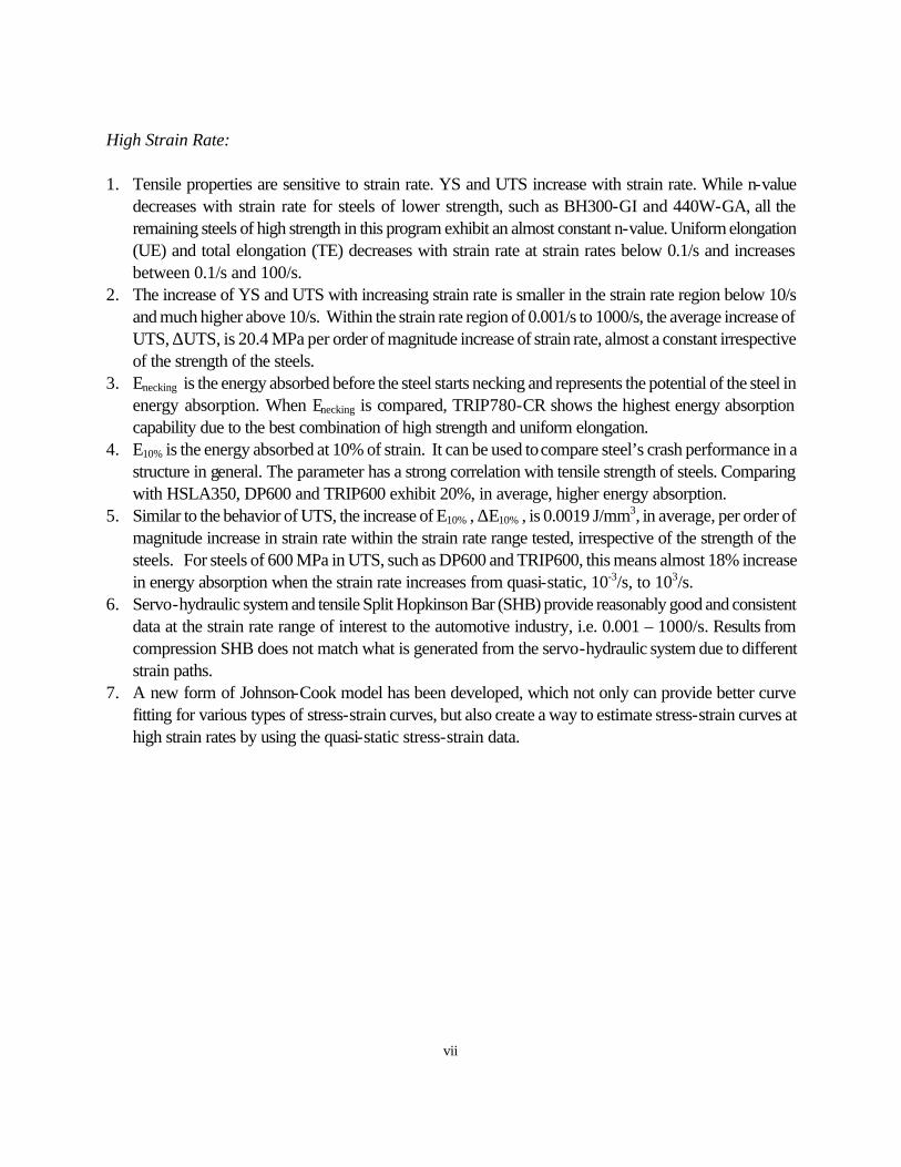
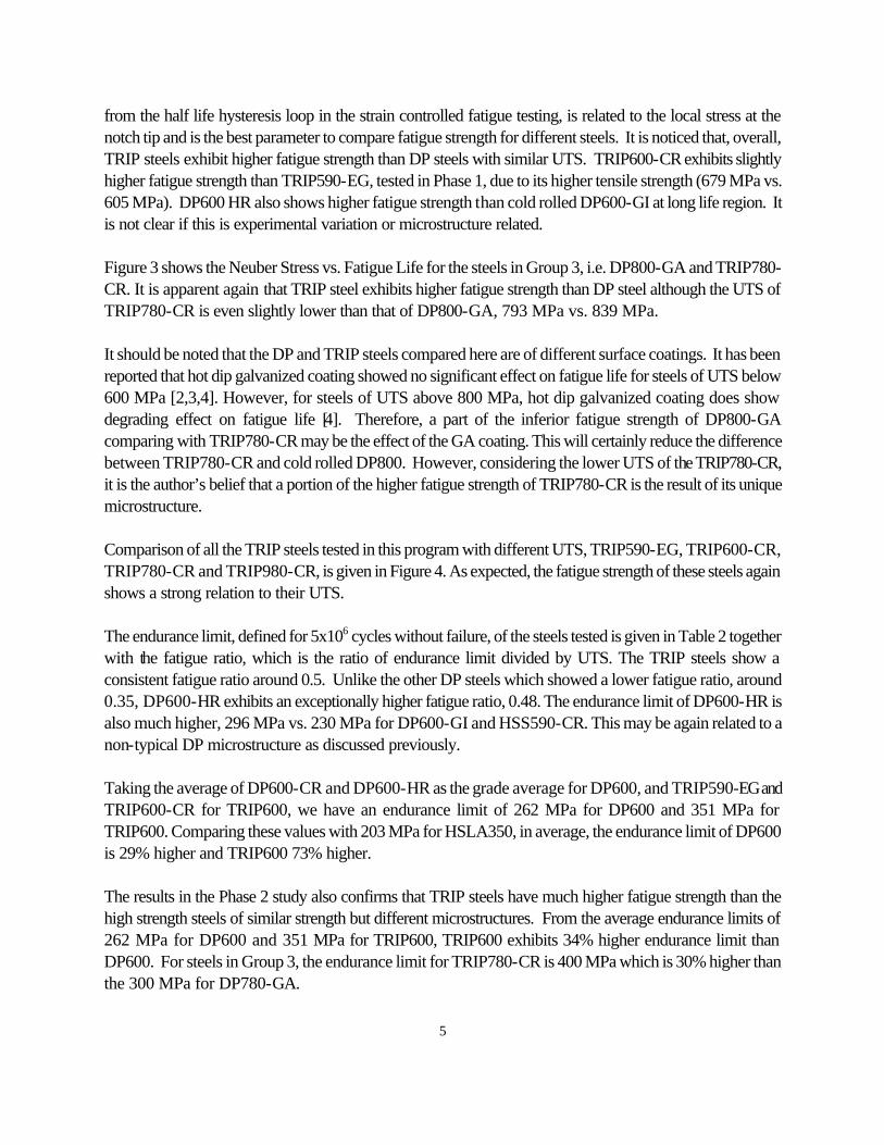
Figure 9 shows the comparison of stress-strain curves for TRIP600-CR at 100/s using the old (load cell) and new (strain gage) methods to measure load. The load cell signal exhibits slightly more oscillation than the strain gage data. However, overall load measurements are fairly comparable for both methods. The slope of the linear section of the stress-strain curve using load cell has been adjusted using the stress-strain curve up to 2% measured by a strain gage in the gage section. The curve using strain gage for load measurement has not, showing a smaller slope. However, in the final data processing, the slope of the curves would be adjusted to the Young’s modulus. The advantage of the new method is more pronounced at 500/s as shown in Figure 10. The stress-strain curve using load cell shows significantly more severe stress oscillation than that using strain gage. The advantage offered by the new method is evident. The stress-strain curve measured by SHB at 500/s is also plotted in Figure 10. Except for the drastic oscillations at the early stage of testing, the overall stress-strain curves from all three test methods are reasonably comparable. The SHB test exhibits a smaller total elongation due to the limited load wave duration in the test setup and the specimen did not break. It was further observed that there was very little difference between 500/s and 1000/s from the SHB test results, probably due to the high strength of the steels tested in Phase 2. Therefore, testing results from SHB are not used in the detail analyses.

14

TRIP600-CR 100/s

0

100

200

300

400

500

600

700

800

900

0 0.1 0.2 0.3 0.4 0.5

Engineering Strain

En

gin

eeri

ng

Str

ess

(MP

a)

100/s Load Cell100/s Strain Gage

Figure 9. Comparison of stress-strain data at 100/s, using load cell vs. strain gage to measure load

TRIP600-CR 500/s

0

200

400

600

800

1000

1200

0 0.1 0.2 0.3 0.4 0.5

Engineering Strain

En

gin

eeri

ng

Str

ess

(MP

a)

500/s Load Cell500/s Strain Gage500/s SHB

Figure 10. Comparison of stress-strain data at 500/s, using load cell, strain gage and SHB, respectively. The SHB specimen did not break due to the limited duration of the stress wave.

15

4.2 Results 4.2.1 Stress-Strain Data at High Strain Rates

The smoothed stress-strain curves at high strain rates for the four grades, tested in Phase 2, are given in Figures 11 through 14. The flow stresses at 6 strain points, 0.005, 0.02, 0.05, 0.1, 0.15 and 0.2 for the four steels are given in Table 3. For the stress-strain results of the seven grades tested in Phase 1, see the Appendix – Phase 1 Report. Tensile properties, including YS, UTS, UE, TE, n value and two energy absorption parameters are summarized in Table 4. For 1000/s, only UTS and UE from SHB are listed. The YS was determined from the stress-strain data below 2% measured by strain gages. The UTS, UE, and TE were obtained from the smoothed stress strain curves. However, raw data was also used when determining the UTS and UE at 500/s and 1000/s in order to avoid the misleading results by load oscillations. The n-value was determined by fitting the smoothed curve for the strain range of 2-5% to uniform elongation. As in Phase 1, energy absorption was characterized using two parameters, Enecking,, and E10% . The former is calculated by

UEUTSYS

*2

+ and represents the energy absorption of a steel grade when deformed before necking,

while the latter represents the energy absorption when deformed to 10% strain. It should be noted that there are larger errors in the tensile properties measured at high strain rates than those measured at the quasi-static strain rate. These inherent system errors are rather significant for properties involving strain measurement, such as UE, TE, and n-value, at 500/s and 1000/s. Therefore, caution must be taken when making any conclusive statement based on the testing results reported here. Since Phase 2 work is focused on DP and TRIP steels, the strain rate dependence of the tensile properties is discussed for all DP and TRIP steels tested in this program, including DP600-GI and TRIP590-EG tested in Phase 1.

16

DP600 HR

0

100

200

300

400

500

600

700

800

900

0 0.05 0.1 0.15 0.2 0.25

True Strain

Tru

e S

tres

s (M

Pa)

0.005/s0.1/s10/s100/s500/s

Figure 11 Smoothed stress-strain curves for DP600-HR at various strain rates

TRIP600-CR

0

200

400

600

800

1000

1200

0 0.05 0.1 0.15 0.2 0.25 0.3

True Strain

Tru

e S

tres

s (M

Pa)

0.005/s0.1/s10/s100/s500/s

Figure 12 Smoothed stress-strain curves for TRIP600-CR at various strain rates

17

TRIP780-CR

0.0

200.0

400.0

600.0

800.0

1000.0

1200.0

0 0.05 0.1 0.15 0.2 0.25 0.3

True Strain

Tru

e S

tres

s (M

Pa)

0.005/s0.1/s10/s100/s500/s

Figure 13 Smoothed stress-strain curves for TRIP780-CR at various strain rates

TRIP980-CR

0

200

400

600

800

1000

1200

1400

0 0.02 0.04 0.06 0.08 0.1 0.12 0.14 0.16

True Strain

Tru

e S

tres

s (M

Pa)

0.005/s0.1/s10/s100/s500/s

Figure 14 Smoothed stress-strain curves for TRIP980-CR at various strain rates

18

Table 3. True Flow Stresses at Various Strain Rates

Steel Grade

Strain Rate (1/s)

σ0.005

(MPa) σ0.02

(MPa) σ0.05

(MPa) σ0.10

(MPa) σ0.15

(MPa) σ0.20

(MPa) 0.005 396 762 557 658 718 766 0.1 432 474 569 669 725 10 490 509 609 709 773 827 100 499 528 626 731 796 851

DP600-HR

500 529 557 526 720 791 0.005 433 464 565 676 750 809 0.1 443 480 587 701 775 832 10 491 522 617 730 811 878 100 529 548 661 782 856 918

TRIP600-CR

500 533 593 699 815 884 935 0.005 512 551 647 761 845 917 0.1 531 579 679 796 882 953 10 586 626 716 834 926 1003 100 603 665 753 862 948 1026

TRIP780-CR

500 621 623 741 887 986 1055 0.005 627 802 942 1060 0.1 669 821 972 1086 10 698 828 986 1134 100 706 879 1021 1151

TRIP980-CR

500 761 793 991 1146

19

Table 4. Tensile Properties at Various Strain Rates

Steel Grade Strain Rate (1/s)

YS (MPa)

UTS (MPa)

UE (%)

TE (%)

n-value (YS+UTS)*UE/2

(J/mm3) E10%

(J/mm3)

0.005 397 628 23.3 36.9 0.216 0.119 0.051 0.1 430 629 20.4 33.4 0.216 0.108 0.052 10 490 677 22.2 34.9 0.215 0.129 0.056 100 500 700 23.1 41.3 0.227 0.139 0.057 500 549 712 22.9 44.0 0.214 0.144 0.059

DP600-HR

1000 709 24.5 0.005 408 668 26.7 39.1 0.253 0.144 0.052 0.1 438 682 22.3 33.3 0.246 0.125 0.054 10 486 721 23.9 36.3 0.238 0.144 0.057 100 527 754 24.3 37.5 0.218 0.156 0.061 500 542 767 24.9 42.9 0.205 0.163 0.064

TRIP600-CR

1000 746 23.0 0.005 498 761 28.2 39.3 0.242 0.178 0.060 0.1 529 782 23.8 33.3 0.228 0.156 0.063 10 594 824 23.9 35.7 0.221 0.169 0.066 100 627 844 25.1 36.1 0.206 0.185 0.071 500 653 865 23.5 42.2 0.210 0.178 0.073

TRIP780-CR

1000 907 27.4 0.005 639 973 15.2 21.5 0.172 0.123 0.085 0.1 672 986 12.1 18.6 0.171 0.100 0.088 10 695 1034 12.7 19.7 0.197 0.110 0.090 100 739 1053 15.8 25.2 0.160 0.142 0.094 500 758 1046 14.6 27.1 0.166 0.131 0.094

TRIP980-CR

1000 1056 14.5

20

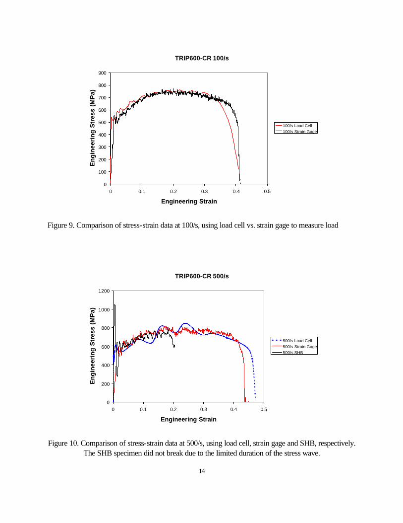
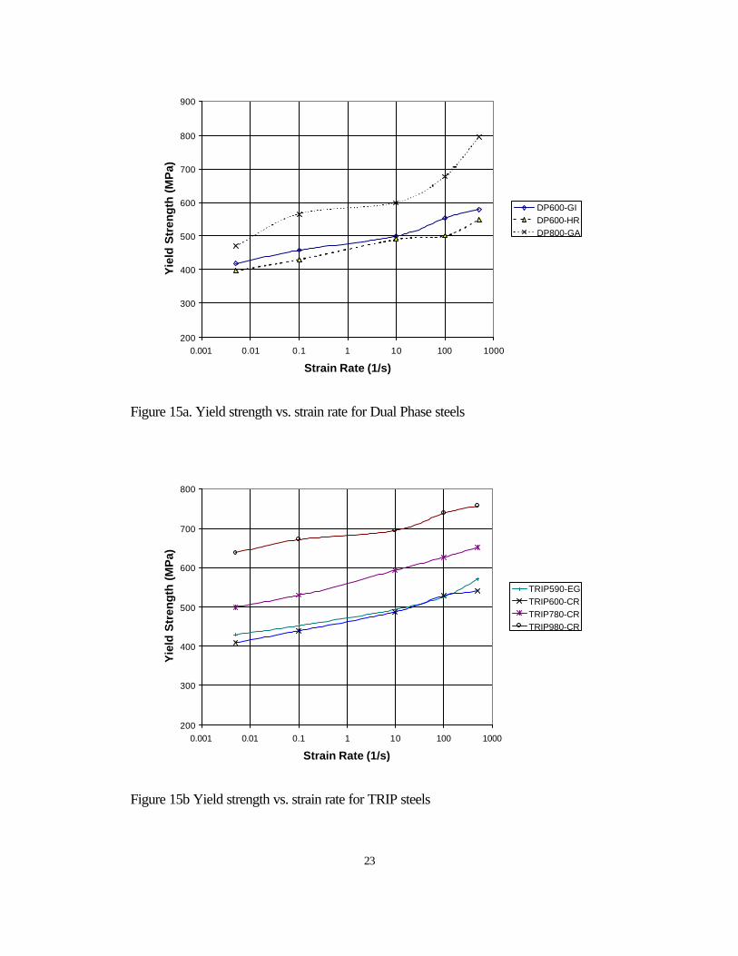
4.2.2 YS and UTS The relationship between YS and strain rate is shown in Figures 15a and 15b for DP and TRIP steels, respectively. As reported in Phase 1, YS increases with strain rate. For most steels, YS increases faster with strain rate at higher strain rates, > 10/s. This is also true for the seven steels tested in Phase 1 (see the Appendix - Phase 1 Report). The same trend was observed for UTS as shown in Figures 16a and 16b for DP and TRIP steels although TRIP980-CR shows slight drop of UTS from 100/s to 500/s, probably caused by testing variability. The increase of UTS per order of magnitude increase in strain rate, ∆UTS, is of great interest in recent years. One of the reasons is that this value seems to be a constant irrespective of the strength of the steel or the type of the steel (e.g. HSLA, DP or TRIP). In Phase 1 work, ∆UTS was shown to be around 22 MPa for strain rates between 0.005/s to 500/s. Using the slope of UTS vs. log ε& , the ∆UTS values for all eleven steels in this program are summarized in Table 5 and is plotted in Figure 17 as a function of UTS at the quasi-static condition. Despite experimental variation, the average of ∆UTS is 20.4 MPa. This is similar to the result in Phase 1. DP600-HR and TRIP980-CR show the lowest ∆UTS. If we exclude these two, the ∆UTS will be 21.3 MPa, very close to the result in Phase 1. 4.2.3 Elongation The dependence of UE and TE on strain rate for DP and TRIP steels is shown in Figures 18a and 18b, and Figures 19a and 19b, respectively. Similar to what was observed in Phase 1 of the investigation, UE decreases first from quasi-static deformation to 0.1/s and then increase with higher strain rates. DP800-GA shows no drop from quasi-static to 0.1/s. At strain rates higher than 100/s, some steels show an increase of uniform elongation and some show a decrease. Moreover, all steels show further increase in TE after 100/s as shown in Figures 19a and 19b. As mentioned earlier, due to the errors involved in the results at 500/s, no conclusion should be made for the behavior at 500/s. Testing for more steel samples is required. 4.2.4 n-value The relationship of n-value with strain rate is shown in Figure 20. No n-values at 500/s are included due to the difficulties in the measurement of n-values at high strain rates. It can be seen that the n-value does not change significantly with strain rate for the DP and TRIP steels tested. TRIP600-CR and TRIP780-CR show slight decrease of n-value with increasing strain rate. 4.2.5 Energy absorption Figures 21 and 22 show the strain rate dependence of the two energy absorption parameters, Enecking , (YS+UTS)*UE/2, in Figure 21 and E10% in Figure 22. Enecking follows the same trend as UE, while E10% increases with strain rate. Furthermore, when Enecking is used to compare the energy absorption for steels, TRIP780-CR and TRIP600-CR are the best among all the DP and TRIP steels tested as the result of their best combination of strength and elongation. However, when E10% is used, TRIP980-CR exhibits the best

21

energy absorption performance, DP800-GA the second, and TRIP780-CR the third. The higher the UTS, the better the energy absorption performance as shown in Figure 23 for 100/s and 500/s. The energy absorption also increases with strain rate in the same way as the UTS. The E10% values at 500/s for DP and TRIP steels in Group 2 are summarized in Table 6 together with that for HSLA350-GI. The average of E10% for DP and TRIP steels in Group 2 is 0.063 J/mm3. Thus, comparing with 0.0527 J/mm3 for HSLA350, DP600 and TRIP600 exhibit 20%, in average, higher energy absorption than HSLA350-GI. It should be noted that the strain value 10% is an arbitrary number and is considered reasonable based on the work by many researchers [5-8] when comparing the steels for crash performance in general. For different structures, different strain values may be needed. For steels of very high strength and UE is less than 10%, strains less than 10%, say 5%, can be used to compare different steels. However, it should be kept in mind that if the total energy under the stress-strain curve before necking or breaking is too low, the steel may buckle or break much earlier before the structure reaches the required energy absorption or displacement. Other steels may perform much better even though their E5% value may be lower. The same situation can happen to E10% , but chance is much higher when E5% is used. Similar to the approach used for UTS, ∆E10%, can be defined as the increase of energy absorption per order of magnitude increase of strain rate and determined from the slope of the ∆E10% vs. log ε& curve. The ∆E10% values are summarized in Table 7 and plotted in Figure 24. It is again almost a constant of 0.0019 J/mm3 irrespective to the steel strength. For steels of UTS 600 MPa in Group 2, the E10% is around 0.063 J/mm3 (see Table 6). This means, if the strain rate increases from 10-3/s to 103/s (6 orders of magnitude increase), the energy absorption, E10% , increases by 0.0114 J/mm3, an increase of almost 18%.

Table 5. Increase of UTS per Order of Magnitude Increase of Strain Rate, in MPa

Phase 1 Phase 2 BH300-GI 20.3 DP600-HR 15.3 440W-GA 22.3 TRIP600-CR 20.6

HSLA350-GI 22.2 TRIP780-CR 20.3 HSS590-CR 23.0 TRIP980-CR 17.0 DP600-GI 24.8

TRIP590-EG 19.3

DP800-GA 18.8 Average of Phase 1

and Phase 2 20.4 MPa

22

Table 6 E 10% at 500/s for DP and TRIP steels in Group 2 in comparison with HSLA350-GI

Grade E10% , in J/mm3

HSLA350-GI 0.0527

DP600-GI 0.0697

DP600-HR 0.0590

TRIP590-EG 0.0606

TRIP600-CR 0.0640

Table 7. Increase of E10% per Order of Magnitude Increase of Strain Rate, in J/mm3

Phase 1 Phase 2

BH300-GI 0.0021 DP600-HR 0.0015

440W-GA 0.0020 TRIP600-CR 0.0020

HSLA350-GI 0.0022 TRIP780-CR 0.0024

HSS590-CR 0.0019 TRIP980-CR 0.0019

DP600-GI 0.0015

TRIP590-EG 0.0017

DP800-GA 0.0018 Average of Phase 1

and Phase 2 0.0019

23

200

300

400

500

600

700

800

900

0.001 0.01 0.1 1 10 100 1000

Strain Rate (1/s)

Yie

ld S

tren

gth

(M

Pa)

DP600-GIDP600-HRDP800-GA

Figure 15a. Yield strength vs. strain rate for Dual Phase steels

200

300

400

500

600

700

800

0.001 0.01 0.1 1 10 100 1000

Strain Rate (1/s)

Yie

ld S

tren

gth

(M

Pa)

TRIP590-EGTRIP600-CRTRIP780-CRTRIP980-CR

Figure 15b Yield strength vs. strain rate for TRIP steels

24

400

500

600

700

800

900

1000

0.001 0.01 0.1 1 10 100 1000 10000

Strain Rate (1/s)

Ten

sile

Str

eng

th (

MP

a)

DP600-GIDP600-HRDP800-GA

Figure 16a. Ultimate tensile stress vs. strain rate for Dual Phase steels

400

500

600

700

800

900

1000

1100

0.001 0.01 0.1 1 10 100 1000 10000

Strain Rate (1/s)

Ten

sile

Str

eng

th (

MP

a)

TRIP590-EGTRIP600-CRTRIP780-CRTRIP980-CR

Figure 16b Ultimate tensile strength vs. strain rate for TRIP steels

25

0

5

10

15

20

25

30

35

40

45

50

200 300 400 500 600 700 800 900 1000 1100

UTS at 0.005/s, MPa

Incr

ease

of

UT

S, M

Pa

Figure 17 Increase in UTS per order of magnitude increase in strain rate vs. quasi-static UTS

0

5

10

15

20

25

30

0.001 0.01 0.1 1 10 100 1000

Strain Rate (1/s)

Un

ifo

rm E

lon

gat

ion

(%

)

DP600-GI

DP600-HR

DP800-GA

Figure 18a Uniform elongation vs. strain rate for Dual Phase steels

26

0

5

10

15

20

25

30

0.001 0.01 0.1 1 10 100 1000

Strain Rate (1/s)

Un

ifo

rm E

lon

gat

ion

(%

)

TRIP590-EGTRIP600-CRTRIP780-CRTRIP980-CR

Figure 18b Uniform elongation vs. strain rate for TRIP steels

0

5

10

15

20

25

30

35

40

45

50

0.001 0.01 0.1 1 10 100 1000

Strain Rate (1/s)

To

tal E

lon

gat

ion

(%

)

DP600-GIDP600-HRDP800-GA

Figure 19a Total elongation vs. strain rate for Dual Phase steels

27

0

5

10

15

20

25

30

35

40

45

50

0.001 0.01 0.1 1 10 100 1000

Strain Rate (1/s)

To

tal E

lon

gat

ion

(%

)

TRIP590-EGTRIP600-CRTRIP780-CRTRIP980-CR

Figure 19b Total elongation vs. strain rate for TRIP steels

0.1

0.15

0.2

0.25

0.3

0.001 0.01 0.1 1 10 100 1000

Strain Rate (1/s)

n-V

alu

e

DP600-GIDP600-HRDP800-GATRIP590-EGTRIP600-CRTRIP780-CRTRIP980-CR

Figure 20 n-values vs. strain rate for Dual Phase and TRIP steels

28

Energy Absorption Before Necking

0.000

0.020

0.040

0.060

0.080

0.100

0.120

0.140

0.160

0.180

0.200

0.001 0.01 0.1 1 10 100 1000

Strain Rate (1/s)

(TS

+YS

)*U

E/2

(J/

mm

3 )

DP600-GIDP600-HRDP800-GATRIP590-EGTRIP600-CRTRIP780-CRTRIP980-CR

Figure 21 Energy absorption before necking per unit volume, Enecking, vs. strain rate.

Energy Absorption at 10% Strain

0

0.01

0.02

0.03

0.04

0.05

0.06

0.07

0.08

0.09

0.1

0.001 0.01 0.1 1 10 100 1000

Strain Rate (1/s)

E 1

0% (J

/mm

3 ) DP600-GIDP600-HRDP800-GATRIP590-EGTRIP600-CRTRIP780-CRTRIP980-CR

Figure 22 Energy absorption below 10% strain, E10% , vs. strain rate

29

0

0.01

0.02

0.03

0.04

0.05

0.06

0.07

0.08

0.09

0.1

200 300 400 500 600 700 800 900 1000 1100

UTS at 10-3/s,MPa

E10

% ,

J/m

m3

100/s500/s

Figure 23 Relationship between E10% and UTS at 10-3/s

0

0.0005

0.001

0.0015

0.002

0.0025

0.003

0.0035

0.004

200 300 400 500 600 700 800 900 1000 1100

UTS at 0.005/s, MPa

Incr

ease

of

E 10%

, J/

mm

3

Figure 24 Increase of E10% per order of magnitude increase in strain rate vs. quasi-static tensile

strength

30

5. Conclusions From the testing results of Phase 1 and Phase 2 in this program, the following conclusions can be drawn: Fatigue 1. In general, fatigue strength has a strong correlation with tensile strength. The higher the tensile strength,

the higher the fatigue strength. Thus, AHSS, such as HSS590, DP600 and TRIP600, exhibited better fatigue strength than the conventional high strength steel of similar yield strength, HSLA350.

2. TRIP steels exhibited significantly better fatigue strength than steels of similar tensile strength but different microstructures. Phase transformation of retained austenite during cyclic deformation may provide additional strengthening to resist fatigue failure.

3. Notch endurance limit increases with increasing tensile strength. For DP and TRIP steels, the increase diminishes for steels of UTS from 600 MPa to 800 MPa for hot dip galvanized steels and from 800 MPa to 1000 MPa for cold rolled bare steels.

High strain rate 4. Tensile properties change with increasing strain rate:

• YS and UTS increases with strain rate • N-value decreases with strain for steels of lower strength, such as BH300 and 440W. For

steels of higher strength in this program, n-value does not change significantly with strain rate • TE and UE decreases with strain rate between 0.001/s to 10/s and increases when the strain

rate is higher than 10/s. 5. ∆UTS, the increase of UTS per order of magnitude increase in strain rate, is almost a constant, 20.4

MPa for all the steels tested within the strain rate range of 0.001/s to 500/s irrespective to their strength and type of the steel.

6. The relationship between the energy absorption parameters, Enecking, and strain rate follows the same trend as UE. TRIP steels exhibit the best energy absorption capability due to the best combination of UTS and UE.

7. The energy absorption below 10% of strain, E10%, increases with strain rate. The parameter shows a strong relationship with UTS of steels. In average, DP600 and TRIP600 exhibited 20% higher energy absorption than HSLA350.

8. When strain rate increases by an order of magnitude, E 10% increases by 0.0019 J/mm3 in average within the range of strain rates tested for all steels tested in this program. For steels of 600 MPa in UTS, such as DP600 and TRIP600, this means almost 18% increase in energy absorption when the strain rate increases from quasi-static, 10-3/s, to 103/s.

9. Servo-hydraulic system and tensile Split Hopkinson Bar (SHB) provide reasonably good and consistent

data at the strain rate range of interest to the automotive industry, i.e. 0.001 – 1000/s. Results from compression SHB does not match what is generated from the servo-hydraulic system due to different

31

strain paths. 10. A new form of Johnson-Cook model has been developed, which not only can provide better curve

fitting for various types of stress-strain curves, but also create a way to estimate stress-strain curves at high strain rates by using the quasi-static stress-strain data

6. References [1] Testing Procedures for Strain Controlled Fatigue Test (Supplement Instructions for A/SP Sheet Steel

Fatigue Program), February 1998, Auto/Steel Partnership [2] R. A. Chernenkoff, R. G. Davies, and A. R. Krause, “Fatigue Characteristics of Galvannealed Steel

Sheet”, in “Proceedings of International Symposium on Interstitial Free Sheet Steet: Processing, Fabrication and Properties”, ed. By L. E. Collins and D. L. Baragar, Canadian Institute of Mining, Metallurgy and Petroleum, 1991

[3] B. Yan, “Fatigue Performance of Zinc Coated Hi-Form Steels (HiForm 50 and HiForm 60)”, Ispat Inland Inc. internal memorandum, 1993

[4] T. Nilsson, G. Engberg and H. Trogen, “Fatigue Properties of Hot-Dip Galvanized Steels”, Scandinavian Journal of Metallurgy, 18, pp. 166-175, 1989

[5] K. Sato, A. Yoshitake and Y. Hosoya, “A Study on Improving the Crashworthiness of Automotive Parts by Using Hat Square Columns”, IBEC ’97, Interior, Safety and Environment, pp. 89-97, 1997

[6] Y. Ojima, Y. Shiroi, Y. Taniguchi, and K. Kato, “Application to Body Parts of High-Strength Steel Sheet Containing Large Volume Fraction of Retained Austenite”, Society of Automotive Engineers, Warrendale, PA, paper# SAE 980954, 1998

[7] K. Miura, S. Takagi, T. Hira and O. Furukimi, and S. Tanimura, “High Strain Rate Deformation on High Strength Sheet Steels for Automotive Parts”, Society of Automotive Engineers, Warrendale, PA, paper# SAE 980952, 1998

[8] ULSAB-AVC Program, Technical Transfer Dispatch #6, 05-01-2001, ULSAB-AVC Body Structure Materials, AISI, ULSAB-AVC, 2001

32

7. Appendix

Phase 1 Report

CHARACTERIZATION OF FATIGUE AND CRASH PERFORMANCE OF NEW GENERATION HIGH STRENGTH STEELS FOR AUTOMOTIVE APPLICATIONS

By

Benda Yan, Principal Investigator Dennis Urban, Program Manager

July 2002

Ispat Inland Inc., Research Laboratories 3001 E. Columbus Drive East Chicago, IN 46375

33

TABLE OF CONTENTS

Page Table of Contents…………………………………………………………………………… 33 List of Figures……………………………………………………………………………… 34 List of Tables………………………………………………………………………………. 36 Executive Summary ……………………………………………………………………….. 37 1. Introduction………………………………………………………………………… 39 2. Steel Grades………………………………………………………………………… 39 3. Testing Programs…………………………………………………………………… 42 4. Fatigue Behavior…………………………………………………………………… 42 4.1 Experiments………………………………………………………………… 42

4.1.1 Strain controlled fatigue test………………………………………… 42 4.1.2 Notched fatigue test…………………………………………………. 42

4.2 Results……………………………………………………………………… 44 4.2.1 Strain-controlled fatigue……………………………………………… 44 4.2.2 Fatigue of notched specimens………………………………………… 48

5. High Strain Rate Behavior…………………………………………………………. 50 5.1 Experiment……………………………………………………………………… 50 5.2 Data reduction…………………………………………………………………… 53

5.2.1 Results from servo-hydraulic systems………………………………… 54 5.2.2 Results from Split Hopkinson Bar (SHB) systems…………………… 59

5.3 Results………………………………………………………………………….. 61 5.3.1 Comparison of various testing methods……………………………… 61 5.3.2 Stress-strain data at high strain rates………………………………… 64 5.3.3 Strain rate effect……………………………………………………… 72 5.3.4 Strain rate sensitivity………………………………………………… 80

5.4 Constitutive model…………………………………………………………….. 81 6. Conclusions………………………………………………………………………… 87 7. References………………………………………………………………………….. 88

34

LIST OF FIGURES Figure A1 Engineering stress-strain curves. …………………………………………… 41 Figure A2 True stress-strain curves…………………………………………………… 41 Figure A3 Configuration of smooth fatigue specimen………………………………… 43 Figure A4 Configuration of notched fatigue specimen, Kt = 2.5……………………… 43 Figure A5 Notched specimen with crack detection gages……………………………… 43 Figure A6 Strain-life curves……………………………………………………………. 45 Figure A7 Eεσ∆∆ vs. life curves …………………………………………………… 45 Figure A8 Variation of strain - life curves for three coils of cold rolled DQSK……… 46 Figure A9 Eεσ∆∆ - life curves to compare HSS590, DP600, TRIP590 with HSLA350…………………………………………………………….. 46 Figure A10 ∆S/2 vs. 2Nf curves for notched fatigue tests……………………………… 49 Figure A11 ∆S/2 vs. 2Nf curves for HSS590, DP600 and TRIP590 vs. HSLA350……. 49 Figure A12a) Tensile specimen used for servo-hydraulic system………………………… 52 Figure A12b) Specimen used for compression SHB……………………………………… 52 Figure A12c) Specimen used for tension SHB………..………………………………….. 52 Figure A13 Schematic illustration of compression SHB system………………………. 53 Figure A14 Schematic illustration of tension SHB system……………………………. 53 Figure A15 Stress and strain raw data from servo-hydraulic tests……………………… 54 Figure A16 A typical displacement vs. time plot………………………………………. 56 Figure A17 Two engineering stress-strain curves. The short one directly from strain gage measurement. The full curve calculated from displacement .… 56 Figure A18 Shifted engineering stress-strain curve……………………………………… 57 Figure A19 Polynomial fitting to get smoothed stress-strain curve……………………… 57 Figure A20 Shifted and smoothed engineering stress-strain curve……………………… 58 Figure A21 Smoothed true stress-strain curve………………………………………….. 58 Figure A22 Stress and strain data from SHB tests……………………………………… 59 Figure A23 Strain rate vs. time for tension and compression SHB tests………………… 60 Figure A24 Polynomial smoothing of tension SHB data………………………………… 60 Figure A25 Comparison of true stress-strain curves between tension and compression SHB for 440W at 1000/s………………………………… 62 Figure A26 Comparison of true stress-strain curves between tension and compression SHB for DP800 at 500/s………………………………… 62 Figure A27 Comparison of true stress-strain curves between servo-hydraulic and SHB tests for 440W at 500/s…………………………………………… 63 Figure A28a) Stress-strain data from strain gages for BH300, showing little systematic changes of the modulus of elasticity with strain rates…………… 65

35

Figure A28b) Stress-strain data from strain gages for HSLA350, showing little systematic changes of the modulus of elasticity with strain rates…………… 65 Figure A29a) Smoothed true stress-strain curves at various strain rates for BH300……… 66 Figure A29b) Smoothed true stress-strain curves at various strain rates for HSLA350…… 66 Figure A29c) Smoothed true stress-strain curves at various strain rates for 440W………… 67 Figure A29d) Smoothed true stress-strain curves at various strain rates for HSS590……… 67 Figure A29e) Smoothed true stress-strain curves at various strain rates for TRIP590…….. 68 Figure A29f) Smoothed true stress-strain curves at various strain rates for DP600……… 68 Figure A29g) Smoothed true stress-strain curves at various strain rates for DP800………. 69 Figure A30 Yield stress vs. strain rate…………………………………………………… 73 Figure A31 Ultimate tensile stress vs. strain rate………………………………………… 73 Figure A32 Uniform elongation vs. strain rate…………………………………………… 74 Figure A33 Total elongation vs. strain rate………………………………………………. 74 Figure A34 n-value vs. strain rate………………………………………………………… 75 Figure A35 Energy absorption before necking per unit volume vs. strain rate..………… 75 Figure A36 Energy absorption before necking per unit volume vs. strain rate for HSS590, DP600 and TRIP590 comparing with HSLA350………………… 76 Figure A37 Energy absorption below 10% strain, E10% , vs. strain rate………………… 77 Figure A38 Energy absorption below 10% strain, E10% vs. quasi-static UTS…………… 77 Figure A39 σ500/σ0.005 vs. quasi-static UTS…………………………………………….. 79 Figure A40 σ500 - σ0.005 vs. quasi-static UTS…………………………………………… 79 Figure A41a Comparison between the smoothed experimental data and model prediction (dashed lines) for BH300…………………………… 83 Figure A41b Comparison between the smoothed experimental data and model prediction (dashed lines) for 440W……………………………… 83 Figure A41c Comparison between the smoothed experimental data and model prediction (dashed lines) for HSLA350………………………… 84 Figure A41d Comparison between the smoothed experimental data and model prediction (dashed lines) for HSS590…………………………… 84 Figure A41e Comparison between the smoothed experimental data and model prediction (dashed lines) for DP600…………………………… 85 Figure A41f Comparison between the smoothed experimental data and model prediction (dashed lines) for TRIP590…………………………… 85 Figure A41g Comparison between the smoothed experimental data and model prediction (dashed lines) for DP800…………………………… 86

36

LIST OF TABLES Table A1 Tensile Properties …………………………………………………………… 40 Table A2 Fatigue Properties…………………………………………………………… 47 Table A3 True flow stresses at various strains rates………………………………….. 70 Table A4 Tensile properties at various strain rates…………………………………… 71 Table A5 Cys and Cuts for simplified Johnson-Cook Model………………….………… 80 Table A6 Parameters for the New Constitutive Model…………………………..……. 82

37

EXECUTIVE SUMMARY Fatigue and high strain rate properties are the important attributes for advanced high strength steels (AHSS) because many of them will be used for structural applications which are subjected to cyclic loading and are often safety critical. In this study, material properties under cyclic and impact loading conditions were investigated for six AHSS steel grades[including Dual-phase (DP) steels, Transformation Induced Plasticity (TRIP) steels, Bake Hardenable (BH) steels, and conventional High Strength Steels (HSS) such as, High Strength Low Alloy (HSLA) steels] with a conventional high strength steel, HSLA350-GI as a benchmark. The six steel grades are: BH300-GI, 440W-GA, HSS590-CR, TRIP590-EG, DP600-GI and DP800-GA. The terms GI, GA, CR, EG denote surface coatings of hot dip galvanized, galvanealed, no coating (cold rolled surface) and electrogalvanized, respectively. The fatigue properties not only include the strain controlled fatigue data, but also fatigue properties of specimens with a stress raiser. While the former provides the material fatigue input for fatigue life prediction, the latter offers information on the notch sensitivity since high strength steels are generally more notch sensitive. Based on the tensile strength, these steels can be categorized into three groups. Group 1 has yield strength 300-350 MPa and UTS 400-440 MPa, and includes BH300, 440W and HSLA350. Group 2 has a minimum UTS of 590-600 MPa, and includes HSS590, DP600 and TRIP590. Group 3 has minimum UTS of 780-800 MPa. DP800 is the only grade in the first phase of the study. The steels in Group 2 have similar yield strength to HSLA350 and are the potential alternative steels for structural applications. Fatigue: The results show that steels in the same group exhibit similar fatigue strength. The fatigue strength increases with the tensile strength of the steels. Therefore, Group 2 exhibits higher fatigue strength than Group 1. Group 3 shows the highest fatigue strength. The results show no significant difference in notch sensitivity for the steels studied except DP800. The relative ranking of these three groups of steels in fatigue strength does not change even when stress raisers are present. There are two exceptions. First, TRIP590 exhibits significantly higher fatigue strength than the steels in the same group, i.e. HSS590 and DP600. This is attributed to the additional strengthening during cyclic deformation when the retained austenite is transforming to martensite. This exceptionally high fatigue strength is maintained when stress raisers are present. Second, DP800 exhibits higher notch sensitivity than the other steels tested in the high cycle region. This results in a reduced endurance limit when stress raisers are present and is related to its high tensile strength. Comparing AHSS steels in Group 2 with HSLA350, the endurance limits of HSS590 and DP600 are 15% higher than that for HSLA350. TRIP590 exhibits a surprisingly 68% higher endurance limit than HSLA350. The existence of a notch in the specimen does not significantly change the advantage of the AHSS over HSLA350.

38

High Strain Rate: The strain rate sensitivity, which is normally defined as the percentage increase of the flow stress due to the increase of strain rate, decreases with increasing tensile strength of the steel. Therefore, the steels in Group 1 are more strain rate sensitive than the steels in Group 2, and steels in Group 3, DP800, shows the lowest strain rate sensitivity due to its high tensile strength. Steels in the same group, such as BH300, 440W and HSLA350 in Group 1, exhibit similar strain rate sensitivity. However, the increment of UTS due to the increasing strain rate is almost constant for all the steels tested, around 22 MPa for each strain rate increase in order of magnitude in average. Since there is no proven parameter to truly represent the capability of energy absorption during a crash

event, two parameters are used in this study, the energy absorbed before necking, UEUTSYS

*2

+, and the

energy absorbed at 10% of strain, E10%. The former represents the potential of a steel to absorb energy, while the latter can be used to compare crash performance of steels when a certain amount of energy is required, or a certain amount of deformation is allowed, in a structure.

When UEUTSYS

*2

+ is used, the TRIP590 shows the highest potential for crash energy absorption as the

result of its exceptionally high elongation. HSLA350 shows the worst potential for energy absorption capability. At 100/s, the capability of energy absorption for the steels in Group 2, HSS590, DP600 and TRIP590, is 51%, 81% and 100% higher, respectively, than that for HSLA350. However, for E10% , the energy absorbed up to 10% of strain in a tensile test is related to the UTS of the steel. The improvement of energy absorption by using HSS590, DP600 and TRIP590 over HSLA350 is reduced to 17%, 34% and 17%, respectively, much less than the steels potentially can offer. Evaluation of the testing methods used in this study shows that servo-hydraulic system and tension Split Hopkinson Bar (SHB) can produce testing results of reasonable quality for the range of strain rates observed during a crash, from quasi-static to 1000/s. Results generated by compression Split Hopkinson Bar do not match well with the data generated by the servo-hydraulic system due to the difference in loading path. Furthermore, a new constitutive model, modified from the Johnson-Cook model, has been developed. The model offers more flexibility to fit experimental results at high strain rates and the potential to estimate stress-strain data at high strain rates from the quasi-static tensile stress strain data.

39

1. Introduction The Project titled "Characterization of Fatigue and Crash Performance of a New Generation of High Strength Steels" started in January 2001. With the support of the AISI Automotive Applications Committee (AISI/AAC) and Auto/Steel Partnership (A/SP) Advanced High Strength Steel Team, the first phase of the project has been successfully completed. Altogether, fatigue and high strain rate data have been generated for six advanced high strength steels (AHSS) and a conventional high strength steel that is used for benchmark. This report documents technical details and findings. 2. Steel Grades Steel grades for this project were selected by the A/SP Advanced High Strength Steel Team. Six Advanced High Strength Steel (AHSS) grades were selected. These are 1.4mm GA 440W, 1.43mm GI BH300, 1.40mm CR HSS590, 1.24mm GI DP600, 1.19mm GA DP800 and 1.45mm EG TRIP590. A conventional high strength steel, 1.6mm GI HSLA350, was also selected for benchmarking. Surface condition of the steels is described by the following designation: GA is galvannealed, GI is hot dip galvanized, EG is electrogalvanized, and CR is cold rolled (bare, no coating). The numbers in the grades denote the minimum ultimate tensile strength (UTS) except GI BH300 and HSLA350, where the numbers are the minimum yield strength (YS). North American steel companies supplied six of the seven grades. However, no commercial TRIP steel products were available in North America when the project started in early 2001. POSCO was then solicited to supply TRIP steels. To protect the product confidentiality for the steel suppliers, no chemical compositions are given. Tensile tests were conducted according to ASTM E8 and the results are summarized in Table A1. Engineering and true stress-strain curves are shown in Figures A1 and A2, respectively. Based on the tensile properties, the steels tested can be categorized into three groups: Group 1 has YS of 300-350 MPa and UTS of 400-440 MPa. This includes BH300, HSLA350 and 440W. While the HSLA350 shows the highest YS among the steels tested, the 440W shows the highest UTS. The BH300 exhibits the highest total elongation (TE). Group 2 has a minimum UTS of 590-600 MPa. This group includes HSS590, DP600 and TRIP590. Tensile tests show that the DP600 supplied exhibits an UTS of 666 MPa that is much higher than the other two grades, 608 MPa and 605 MPa for HSS590 and TRIP590, respectively. As expected, the TRIP590 exhibits the highest TE, 32%. Group 3 has a minimum UTS of 780-800 MPa. There is only one grade in the current phase, DP800. This is the steel grade with the highest strength in all the steel tested in this phase. Since the steels in Group 2 have similar yield strength, 350-400MPa, as the conventional high strength steel, HSLA350, they are considered extensively today as the alternative steels to replace HSLA350 for automotive structural applications to reduce weight. Therefore, comparisons are often made between these steels.

40

Table A1 Tensile Properties (As received, ASTM E8, "L" direction)

Group 1 Group 2 Group 3

BH300 GI

440W GA

HSLA350 GI

HSS590 CR

DP600 GI

TRIP590 EG

DP800 GA

YS (MPa)

309 326 356 431 412 428 462

UTS (MPa)

412 462 441 608 666 605 839

TE (%)

35.8 29.0 28.1 24.5 23.2 32.0 17.9

UE (%)

20.4 16.3 15.8 15.1 15.3 22.6 12.3

n (6-12)

0.19 0.18 0.13 0.17 0.16 0.20 0.13

41

0

100

200

300

400

500

600

700

800

900

0.00 0.05 0.10 0.15 0.20 0.25 0.30 0.35

Engineering Strain

En

gin

eeri

ng

Str

ess,

MP

a

BH300

DP800

DP600

TRIP590

HSS590440W

HSLA350

Figure A1 Engineering stress-strain curves.

Figure A2 True stress-strain curves

0

100

200

300

400

500

600

700

800

900

1000

0 0.05 0.1 0.15 0.2 0.25

True Strain

Tru

e S

tres

s, M

Pa

BH300

HSLA350440W

HSS590

TRIP590

DP800

DP600

42

3. Testing Programs The purpose of this project is to generate fatigue and crash data for the AHSS. Fatigue tests include strain controlled fatigue test using smooth specimens and notched fatigue test using notched specimens. Fatigue data from notched specimens can be used to study the notch sensitivity of steels. The crash data originally included intrinsic material stress-strain data at high strain rates and crush test data for conical tubes. It was realized later that Auto/Steel Partnership (A/SP) High Rate Group is working on a similar project to generate crush test data for benchmarking, so it was approved by AISI/AAC that this project will not perform crush test. Therefore, only the high strain rate results are reported. 4. Fatigue 4.1 Experiments 4.1.1 Strain controlled fatigue test Strain controlled fatigue tests were conducted in accordance with ASTM E606 and Testing procedures for Strain Controlled Fatigue Testing developed by Auto/Steel Partnership Sheet Steel Fatigue Group [A1]. Testing was conducted on a 3 kip MTS closed-loop servo-hydraulic system using smooth specimens with a total strain amplitude ranging from 0.1% to 0.8%. Three replicates for each strain level were used. The highest amplitude is limited by the strength and thickness of the steel due to the propensity to buckling. The geometry of the specimens is shown in Figure A3. Tests were fully reversed tension-compression and terminated when the tensile load is dropped by 60%, indicating cracks in the specimens. Run-out was defined when no failure occurred after 5 million cycles. 4.1.2 Notched fatigue test Notch sensitivity was tested using center hole specimens with the stress concentration factor, Kt = 2.5. The dimensions of the specimens are shown in Figure A4. Tests were load controlled in accordance with the ASTM E466. The load was fully reversed tension-compression with R = -1, where R = Pmin/Pmax, Pmin is the minimum load and Pmax is the maximum load. Cracks initiated from the edges of the center hole and propagated along the width direction. Notice that the notched specimen has a much larger cross section than the smooth specimen. Therefore, if the same load drop is used to terminate tests, the fatigue life in the notched specimen testing will include much longer crack propagation than in the smooth specimen tests. In order to keep the crack length in the notched fatigue testing similar to that in the smooth specimens, crack detection gages were glued on a surface along both sides of the hole as shown in Figure A5. A circuit was set up in such a way that when the crack propagates past the gage, the gage is broken and testing is terminated. Our experience showed that cracks in smooth specimens were generally around 1mm long when the tests were terminated. The distance between the crack detection gages and the edges of the hole was thus set at 1mm. Practice showed that the crack detection gages worked very well and tests were consistently terminated at crack lengths within 0.9 - 1.2mm. Tests were conducted on a 20 kip MTS closed-loop

43

W = 2.0 ∀ 0.025 L = 7.92∀ 0.1 D = 12.7-0.02 t = thickness of the sheet

Figure A3 Configuration of smooth fatigue specimen

Figure A4 Configuration of notched fatigue specimen, Kt = 2.5

Figure A5 Notched specimen with crack detection gages

90 mm

22 mm4.4mm dia

L

8.0

D

76.2

All dimensions in mm

w

Maintain C/Lof gauge + 0.025

44

servo-hydraulic machine. Again, run-out was defined by 5x106 cycles without failure. 4.2 Results 4.2.1 Strain-controlled fatigue The strain - life plot is shown in Figure A6. In the plot, as is customary in fatigue testing, the number of cycles is replaced by the number of reversals which is twice the number of cycles. Using the elastic and plastic strain components, which are not shown in the plot, the strain-life parameters can be calculated. They are listed in Table A2. The parameters are the input for fatigue life prediction as the material property. As discussed in detail in the previous work by B. Yan et al. [A2], for most engineering parts where applied load is fixed and failure occurs at the stress raiser, the fatigue strength of different steels is better compared using the εσ∆∆E vs. life curve. The ∆σ and ∆ε are the stress and strain range during the test. The parameter, εσ∆∆E , which is first introduced by Neuber [A3] and is related to the local stress at the notch tip by Topper et al. [A4]. This parameter is equivalent to the local elastic stress at the notch tip obtained by FEA simulation when determining fatigue life, it is referred to as the Equivalent Notch Stress. Figure A7 shows the εσ∆∆E vs. life plot for the seven steels tested. The differentiation between the steels is much more apparent than in Figure A6. It should be pointed out that only one set of data was generated for each steel grade. Due to the property variability for steels within a grade, there is also variation of fatigue properties. After testing three coils of the same grade from each steel producer for three producers, the Auto/Steel Partnership Sheet Steel Fatigue Program found that the Scattering Factor for a grade within a producer can be as high as 2.0. The

Scattering Factor is defined as min

max

NN

, where Nmax and Nmin are the maximum and minimum fatigue life,

respectively, for a specified strain amplitude applied [A5]. This means that for a given strain amplitude tested for the three coils, the maximum life can be 4 times the minimum fatigue life in the worst case. Typical strain vs. life curves for three coils of cold rolled DQSK from the same producer are given in Figure A8, showing possible variations of fatigue properties [A5]. With this variability in mind, it can been seen that, in general, each group of steels exhibits similar fatigue strength and the higher the tensile strength, the higher the fatigue strength. The fatigue strengths of the steels in Group 1, BH300, HSLA350 and 440W, are similar. The steels in the second group, i.e. steels with UTS of 590-600 MPa, all show higher fatigue strength than the steels in the first group. And Group 3, DP800 exhibits even higher fatigue strength than Group 2. Within Group 2, the HSS590 and DP600 exhibit similar fatigue strength. However, TRIP590 exhibits exceptionally higher fatigue strength, similar to DP800. This exceptionally high fatigue strength is believed to be the result of progressive phase transformation of retained austenite to martensite during cyclic deformation. This additional strengthening delays crack initiation and propagation processes and therefore improves fatigue life.

45

0.0001

0.0010

0.0100

1000 10000 100000 1000000 10000000

2Nf, Number of Reversals

Str

ain

Am

plit

ud

e440WHSS590HSLA350DP600TRIP590DP800BH300

TRIP590

DP800

DP600

HSS590

440W

HSLA350

BH300

Figure A6 Strain vs. life curves

0

100

200

300

400

500

600

700

800

900

1000

1000 10000 100000 1000000 10000000

Number of Reversals to Failure, 2Nf

BH300440WHSLA350HSS590

DP600TRIP590DP800

DP800

TRIP590

DP600

HSS590HSLA350

440W

BH300

Figure A7 εσ∆∆E vs. life curves

(E∆ε

∆σ)1/

2 , MP

a

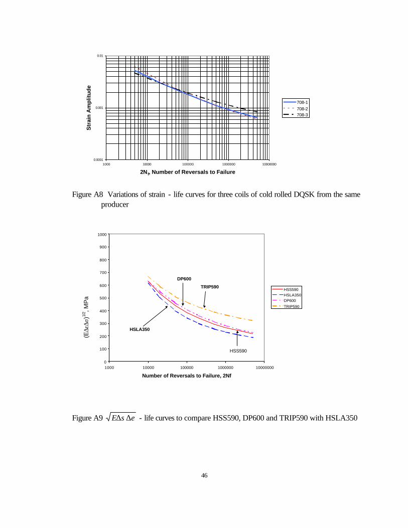
46

Figure A8 Variations of strain - life curves for three coils of cold rolled DQSK from the same

producer

Figure A9 εσ∆∆E - life curves to compare HSS590, DP600 and TRIP590 with HSLA350

(E∆ε

∆σ)1/

2 , MP

a

0.0001

0.001

0.01

1000 10000 100000 1000000 10000000

2N f, Number of Reversals to Failure

Str

ain

Am

plit

ud

e

708-1708-2708-3

0

100

200

300

400

500

600

700

800

900

1000

1000 10000 100000 1000000 10000000

Number of Reversals to Failure, 2Nf

HSS590HSLA350DP600

TRIP590

TRIP590

DP600

HSS590

HSLA350

47

Table A2 Fatigue Properties

BH300 GI

440W GA

HSLA350 GI

HSS590 CR DP600 GI TRIP590 EG

DP800 GA

'fσ (MPa) 549 841 806 886 983 813 1205

'fε 0.969 0.468 1.920 0.480 0.211 0.496 0.104

b -0.063 -0.105 -0.098 -0.095 -0.101 -0.063 -0.101

c -0.614 -0.523 -0.668 -0.538 -0.457 -0.572 -0.394

K' (MPa) 530 966 671 983 1363 871 2104

n' 0.097 0.198 0.133 0.173 0.219 0.109 0.253

Endurance Limit, σe

(MPa) 193 209 203 230 228 336 307

Fatigue Ratio 0.47 0.45 0.46 0.38 0.34 0.56 0.37

Notch Endurance

Limit, σn (MPa)

120 130 125 144 142 178 147

Kf at 107 Reversals

σe/σn 1.61 1.61 1.62 1.60 1.61 1.89 2.09

'fσ - Fatigue strength coefficient

'fε - Fatigue ductility coefficient

b - Fatigue strength exponent c - Fatigue ductility exponent K' - Cyclic strength coefficient n' - Cyclic strain hardening exponent

In Figure A9, HSS590, DP600 and TRIP590 are compared with HSLA350. The advantage of the AHSS over the conventional high strength steel is evident with TRIP590 showing the best fatigue strength. Endurance limits were determined by running additional tests under stress control and the results are also given in Table A2. The endurance limit is the stress amplitude equal and below which no fatigue failure will occur. Along with the endurance limit, the fatigue ratio, that is the ratio of endurance limit/UTS, is also listed. Again, the BH300, 440W and HSLA350 exhibit the similar endurance limits, ∼200 MPa. The endurance limits for HSS590 and DP600 are 15% higher. And the endurance limit for DP800 is 50% higher. The TRIP590 exhibits a endurance limit of 336 MPa, which is 68% higher than those for Group 1, 46% higher than the other two steels in the same group, and even 10% higher than the endurance limit of DP800. It should be noted that the endurance limit was defined by 5x106 cycles without failure. Recent study shows

48

that steel may still fail after 108 to 109 cycles even at stress ranges equal or below the endurance limit [A6, A7]. One thus has to be cautious when using the endurance limit for gigacycle applications. Furthermore, the fatigue properties generated in this study are for the steels in the as-received condition. Since forming strain can affect the tensile properties of the steel, especially for dual phase and TRIP steels, the fatigue strength of the formed part will be different from the steels in the as-received condition. 4.2.2 Fatigue of notched specimens Figure A10 shows nominal stress amplitude, ∆S/2, vs. 2Nf for the steels tested. The nominal stress was calculated by using the net cross section. These are the regression curves from testing data and are shown only within 2000 to 5x106 reversals where testing data are available. For legibility, no data points are shown. The smooth specimen results showed that the steels within a group normally exhibit similar fatigue strength except TRIP590. This is again true for notched specimens as shown in Figure A10. With a center hole of Kt=2.5, BH300, HSLA350 and 440W show similar fatigue strength. Although 440W seems to have lower fatigue strength at the low cycle region and higher fatigue strength at the high cycle region, variations of fatigue strength from coil to coil may eliminate the differences we see from the single-coil data. HSS590 and DP600 also show similar notch fatigue strength. Similar to the base metal fatigue property, TRIP590 again exhibits much higher notch fatigue strength. However, while DP800 exhibits notch fatigue strength higher than DP600 at the low cycle range, in the high cycle region, its fatigue strength decreases quickly and approaching the fatigue strength of DP600. Figure A11 shows the ∆S/2 vs. 2Nf curve for HSS590, DP600 and TRIP590 in comparison with HSLA350. Testing data points are also given in the plot. Similar to the testing results for the smooth specimens as shown in Figure A9, AHSS again show better notch fatigue strength over the conventional high strength steels, HSLA350. The TRIP590 maintains it best fatigue strength. Notch endurance limits with a center hole of Kt 2.5 are also given in Table A2. The notch endurance limits are much lower than the endurance limits for the base metals, indicating a significant drop as the result of the center hole. However, similar to the base metals, HSS590 and DP600 exhibit around 10-15% higher notch endurance limit than steels in Group 1. TRIP590 shows an even higher notch endurance limit. In other words, notch sensitivities of these steels are very similar so that the presence of a notch does not negatively affect the advantage of the AHSS over the conventional high strength steels in fatigue resistance. The only exception is DP800, which shows a notch endurance limit only slightly higher than that of DP600. Fatigue notch sensitivity can be evaluated by the fatigue stress concentration factor, Kf. One simple measurement is by calculating the ratio of the endurance limit over the notch endurance limit, σe/σn. This value represents the notch sensitivity of the steels at high cycle fatigue region. The values are given in Table A2 and show that the notch sensitivity of the steels tested at high cycle region is very similar, with a Kf value of 1.60-1.61, except TRIP590 and DP800. DP800 shows higher notch sensitivity, Kf = 2.09, due to its higher strength. The Kf value of TRIP590 is 1.89 which is higher than the other steels. The reasons for this

49

slightly higher notch sensitivity are not clear. Figure A10 ∆S/2 vs. 2Nf for notched fatigue tests

Figure A11 ∆S/2 vs. 2Nf for HSS590, DP600 and TRIP590 vs. HSLA350

It should be noted that the Kf value is different at different life ranges. Due to the variability of the steel properties as mentioned in this paper, no attempt is made to study the Kf value as a function of fatigue life. However, it can be concluded that, except for DP800, the difference of the notch sensitivity for the steels tested in this study is not significant. It is supported by the fact that the relative fatigue strength of these

0

50

100

150

200

250

300

350

400

450

100 1000 10000 100000 1000000 10000000 100000000

Number of Reversals to Failure

No

min

al S

tres

s A

mp

litu

de,

MP

a

BH300440WHSLA350HSS600DP600TRIP600DP800

0

50

100

150

200

250

300

350

400

450

100 1000 10000 100000 1000000 10000000 100000000

Number of Reversals to Failure

No

min

al S

tres

s A

mp

litu

de,

MP

a

HSLA350(cal)HSS600(cal)DP600(cal)TRIP600(cal)HSLA350(exp)HSS590(exp)DP600(exp)TRIP590(exp)

50

steels is the same with or without notches. 5. High Strain Rate Behavior 5.1 Experiment High strain rate testing is much more complicated than quasi-static testing due to the increasing influence of stress wave propagation. In addition, several different testing methods are available, each is applicable for different ranges of strain rates. Some of the testing techniques are relatively unfamiliar to the steel industry, such as Split Hopkinson Bar (SHB). In the last few years, the Auto/Steel Partnership High Strain Rate Group has coordinated several programs to generate data for a limited number of steel grades. However, questions remain as to what testing method should be used and how the variation in stress-strain data should be treated so that results can be easily used by analysis engineers. In this program, efforts were thus also made to evaluate the two testing methods, servo-hydraulic and SHB systems. Data processing, including data smoothing and curve fitting, will be discussed in detail hoping that this study can provide a basis for the future development of a standard procedure. Six strain rates were selected in this study: 0.001, 0.1, 10, 100, 500 and 1000/s. This is the strain rate range considered most relevant to the automobile crash event. The tests at 0.001, 0.1, 10, 100 and 500/s were performed using servo-hydraulic loading frames at Reinisch-Westfalische Technische Hochschule Aachen (RWTH Aachen, Aachen for short). Tests at strain rates 500 and 1000/s were conducted using Split Hopkinson Bar (SHB), both tension and compression, at the University of Dayton Research Institute (UDRI). The overlap of the 500/s tests was chosen to compare the two testing techniques. All tests were in the “L” direction except the compression SHB tests, where the specimen was tested in the thickness direction. For servo-hydraulic tests, a flat dog-bone type specimen was used with a gage length of 20mm. The specimen drawing is shown in Figure A12a. Three specimens were tested at each condition. Two load cells were used in the loading train, a piezoelectric load cell and an in-house fabricated load cell that is part of the grip system in order to reduce the distance to the specimen. The piezoelectric load cell was used for strain rates less than 5/s, whereas the load cell in the grip was used for higher strain rates. The strain was determined by the displacement divided by the gage length. Comparing the measurement by using an optical extensometer, Aachen claimed that this method is satisfactory. However, in order to obtain direct strain measurements in the small strain region, up to 2%, two out of three specimens were instrumented with a strain gage on each side. During the test, load and displacement were recorded with time. Strains measured directly from the strain gages were also recorded when available. The SHB is routinely used to study mechanical properties of materials at high strain rates in the range of 200 to 105/s. The schematic of the compression SHB system used in this study is shown in Figure A13. The

51

apparatus consists of a striker bar and two pressure bars mounted and aligned longitudinally in bearings that support them rigidly in a horizontal plane. The bars are 12.7 mm in diameter and made of Inconel 718 alloy. The striker bar (0.76 m long) is launched with a torsional spring arrangement and strikes the incident bar (3.7 m long) end to end. This sets up a stress pulse in the incident bar. The magnitude of this incident pulse is proportional to the striker bar velocity and its duration is equal to twice the acoustic transit time of the striker bar. The transit time, t, for this machine is given by

sC

lt s µ315

2

0

=×

= (1)

where ls = 0.76 m, is the length of the striker bar, ρ/0 EC = = 4825 m/s, is the elastic wave velocity, E and ρ is the Young's modulus and density of the pressure bar, respectively. Thus, the maximum strain obtained is 15.7% for 500/s test and 31.5% for 1000/s test. A disc specimen, 3.17mm in diameter as shown in Figure A12b, was used in the compression SHB test and was tested in the thickness direction. The specimen is placed between the two pressure bars. As the compressive pulse is generated in the incident bar, a portion of this incident pulse (ε i) is transmitted through the specimen (ε t) and the remainder is reflected back in the incident bar (εr). The amplitude of the incident, reflected and transmitted pulses are recorded by the strain gages mounted on the two pressure bars as shown in Figure A13. The stress (σ), strain (ε) and strain rate ( ε& ) in the specimen can be calculated from the following equations:

)()( tAA

Et ts

b εσ = (2)

∫=t

r dttLC

t0

0 )(2

)( εε (3)

)(2

)( 0 tLC

t rεε =& (4)

where Ab and As are the cross-sectional area of the pressure bar and the specimen in the gage area, respectively, and L is the gage length of the specimen. The measured strains ε i, εr and ε t have the following relation when the specimen deformed uniformly:

tir εεε −= (5) Strain rate is controlled by changing striker bar velocity. Fine adjustment of the striker bar velocity is practiced until the target strain rate was reached.

52

A= As Received D=6.0 mm B1=10.0 mm H=21.0 mm B2=20.0 mm L1=81.0 mm C=6.0 mm L2=20.0 mm R=10.0 mm

Figure A12(a). Tensile specimen used for servo-hydraulic system

D

D = 3.17 mm (0.125 in) t = steel thickness Figure A12(b). Specimen used for Compression SHB tests

Figure A12(c). Specimen used for tension SHB tests

53

Figure A13. Schematic illustration of the compression SHB system.

Figure A14. Schematic illustration of the tension SHB system. The tension SHB tests follow the same principles as in the compression SHB test. However, because the gage length of the tensile specimen is much longer than that of the compression specimen, the time required for the stress to equilibrate within the specimen is much longer [A8]. UDRI facility uses aluminum pressure bars in the tension SHB system. The test apparatus is shown in Figure A14. A smaller flat dog-bone specimen, with a gage length of 7.62mm, was used for the test. The specimen configuration is given in Figure A12c. The stress, strain and strain rates were obtained from the same equations. Since the maximum strain is only 15.7% for 500/s tests, which is less than the total elongation for the testing materials for this study, specimens were not extended to failure at this strain rate. 5.2 Data Reduction Raw data obtained in servo-hydraulic tests and in SHB tests have different features. Therefore, different data reduction procedures were developed and are discussed here. 5.2.1 Results from the servo-hydraulic tests

54

440W -- Raw data

0

100

200

300

400

500

600

700

0.00 0.10 0.20 0.30 0.40 0.50 0.60 0.70

Strain

Str

ess

(MP

a) 0.005/s0.1/s10/s100/s500/s

Figure A15. Stress and strain data from servo-hydraulic tests

Typical stress-strain curves from the servo-hydraulic systems are given in Figure A15 for 440W. This type of stress strain curve is common for high strain rate testing. There are several features which are compared here to quasi-static tensile curves: § The linear elastic region is delayed by a region of slow increase of stress. § The slope of the linear region is much smaller than the modulus of elasticity at quasi-static testing. § There is a significant load fluctuation at high strain rates which is the result of ringing of the load

measuring system. The causes of the first two phenomena are not totally understood. They can be related to the acceleration of the actuator, the stiffness of the loading system, and the signal delay of the displacement and load due to their different locations. As we were told by Aachen, in order to get data of better quality, two different dampers were used for strain rates of 0.001 and 0.1/s, and strain rates of 10, 100 and 500/s, respectively. This also contributed to the differences between the curves for these two strain rate ranges. Generally, it takes a great deal of tedious data processing to correct the early sections of the stress-strain curve, including slope adjustment. In this study, we rely on the stress-strain data measured by the strain gages as the more accurate information in the elastic region. The following procedures were developed in this study to achieve stress-strain data of good quality (using the 440W data at 500/s for illustration):

1. Verify the strain rate by plotting displacement data versus time. Figure A16 shows a displacement vs. time curve for a 440W specimen tested at a nominal strain rate of 500/s. The slope of the data is 9431mm/s as shown and the strain rate for this test is 9431 (mm/s)/20 (mm) = 472 /s, which is fairly accurate for a 500/s test.

2. Plot the engineering stress-strain data both from direct strain gage measurement and from displacement calculation on the same graph (see Figure A17). The strain gage data terminated

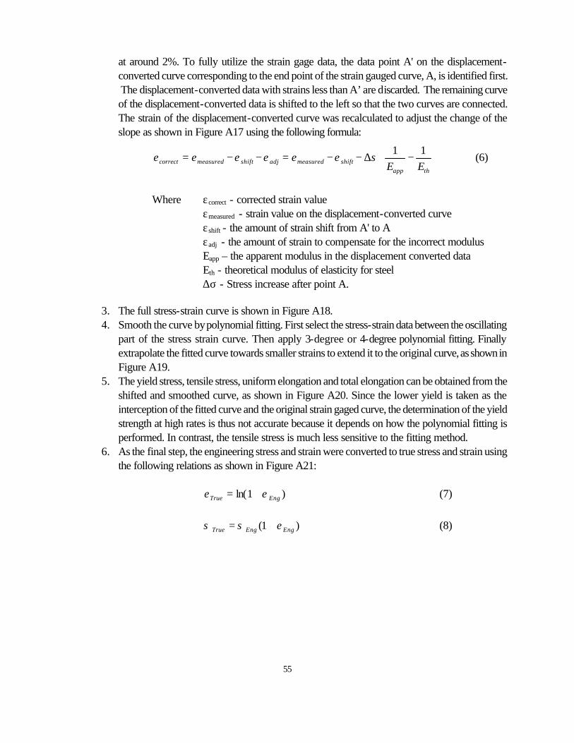
55

at around 2%. To fully utilize the strain gage data, the data point A' on the displacement-converted curve corresponding to the end point of the strain gauged curve, A, is identified first. The displacement-converted data with strains less than A’ are discarded. The remaining curve of the displacement-converted data is shifted to the left so that the two curves are connected. The strain of the displacement-converted curve was recalculated to adjust the change of the slope as shown in Figure A17 using the following formula:

−∆−−=−−=

thappshiftmeasuredadjshiftmeasuredcorrect EE

11σεεεεεε (6)

Where εcorrect - corrected strain value εmeasured - strain value on the displacement-converted curve εshift - the amount of strain shift from A' to A

εadj - the amount of strain to compensate for the incorrect modulus Eapp – the apparent modulus in the displacement converted data Eth - theoretical modulus of elasticity for steel ∆σ - Stress increase after point A.

3. The full stress-strain curve is shown in Figure A18. 4. Smooth the curve by polynomial fitting. First select the stress-strain data between the oscillating

part of the stress strain curve. Then apply 3-degree or 4-degree polynomial fitting. Finally extrapolate the fitted curve towards smaller strains to extend it to the original curve, as shown in Figure A19.

5. The yield stress, tensile stress, uniform elongation and total elongation can be obtained from the shifted and smoothed curve, as shown in Figure A20. Since the lower yield is taken as the interception of the fitted curve and the original strain gaged curve, the determination of the yield strength at high rates is thus not accurate because it depends on how the polynomial fitting is performed. In contrast, the tensile stress is much less sensitive to the fitting method.

6. As the final step, the engineering stress and strain were converted to true stress and strain using the following relations as shown in Figure A21:

)1ln( EngTrue εε += (7)

)1( EngEngTrue εσσ += (8)

56

440W 500/s

y = 9431.1x + 67.36R

2 = 0.9935

66

68

70

72

74

76

78

80

0 0.0002 0.0004 0.0006 0.0008 0.001 0.0012 0.0014

Time (s)

Dis

plac

emen

t (m

m)

Figure A16. A typical plot for displacement vs. time

440W 500/s

0

100

200

300

400

500

600

700

0.00 0.10 0.20 0.30 0.40 0.50 0.60

Engineering Strain

En

gin

ee

rin

g S

tre

ss

(M

Pa

)

Displacement data Strain Gage data

Curve shift (ε shift)

A'

A

Eapp

E th

∆ σ

εadj

Figure A17. Two engineering stress strain curves. The short one directly from strain gage

measurement. The full curve was calculated from displacement.

57

440W 500/s

0

100

200

300

400

500

600

700

0.00 0.05 0.10 0.15 0.20 0.25 0.30 0.35 0.40 0.45 0.50

Engineering Strain

En

gin

eeri

ng

Str

ess

(MP

a)

Figure A18. Shifted engineering stress-strain curve.

440W 500/s

0

100

200

300

400

500

600

700

0.00 0.05 0.10 0.15 0.20 0.25 0.30 0.35 0.40 0.45 0.50

Engineering Strain

En

gin

eeri

ng

Str

ess

(MP

a)

Before smooth Smoothed

Fitting start point Fitting end point

Figure A19. Polynomial fitting to get smoothed stress-strain curve.

58

440W 500/s

0

100

200

300

400

500

600

700

0.00 0.05 0.10 0.15 0.20 0.25 0.30 0.35 0.40 0.45 0.50

Engineering Strain

En

gin

eeri

ng

Str

ess

(MP

a)

Figure A20. Shifted and smoothed engineering stress-strain curve.

440W 500/s

0

100

200

300

400

500

600

700

800

0.00 0.05 0.10 0.15 0.20 0.25 0.30

True Strain

True

Str

ess

(MP

a)

Figure A21. Smoothed true stress - strain curve

59

5.2.2 Results from SHB systems The true stress-strain data for 440W at 500/s are shown in Figure A22 for both tension and compression tests. The tension data show a high degree of oscillation, which is due to the longer stress equilibrium time associated with the longer gage length of the tension specimens. On the other hand, the compression data are much more stable. A close look at the strain rate vs. time data (Figure A23) reveals that the strain rate for the compression SHB tests never stabilized. In fact, it continuously dropped from 200% of the target value at the beginning of the test, 1000/s, to 50% of the target, 250/s, at the end of the test. In contrast, the strain rate in the tension SHB tests was relatively stable. Using a similar smoothing method, stress-strain data for the tension SHB tests at 5% strain or higher were smoothed by 3- or 4- order polynomial fitting. The data with strains less than 5% were discarded due to the instability of the strain rate (see Figure A24). Finally, the true stress and true strain were calculated and plotted. No smoothing was needed for the compression SHB results.

440W 500/s SHB

0

100

200

300

400

500

600

700

800

900

1000

0.00 0.02 0.04 0.06 0.08 0.10 0.12 0.14 0.16 0.18 0.20

True Strain

True

Str

ess

(MP

a)

TensionCompression

Figure A22. Stress and strain data from SHB tests

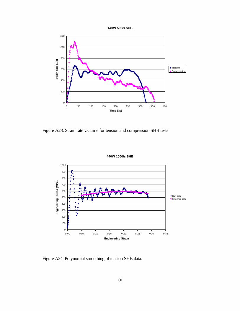
60

440W 500/s SHB

0

200

400

600

800

1000

1200

0 50 100 150 200 250 300 350 400

Time (µs)

Str

ain

rat

e (1

/s)

TensionCompression

Figure A23. Strain rate vs. time for tension and compression SHB tests

440W 1000/s SHB

0

100

200

300

400

500

600

700

800

900

1000

0.00 0.05 0.10 0.15 0.20 0.25 0.30 0.35

Engineering Strain

En

gin

eeri

ng

Str

ess

(MP

a)

Raw dataSmoothed data

Figure A24. Polynomial smoothing of tension SHB data.

61

5.3 Results 5.3.1 Comparison of Various Testing Methods As shown in Figure A22, there are significant differences in the true stress-strain curves between the tension and compression SHB tests. It is speculated that the differences are mainly due to the different loading modes. In the tension SHB test, the steel is subjected to uniaxial tensile loading, whereas in the compression SHB test a compressive load is applied through thickness, which is equivalent to a biaxial in-plane stretch. Yan and et al. showed that the yield strength of an 8% biaxially stretched IF steel is 40% higher than the 8% flow stress during a tensile test (375 MPa vs. 266 MPa) [A2]. This indicates that the flow stress at a certain effective strain can be quite different when the deformation is achieved by two different strain paths. Anisotropy can also contribute to the difference. However, its contribution decreases as the r-value approaches 1.0, as for many high strength steels. An additional factor that may contribute to the difference is the surface friction, which might affect the compression tests but not the tension test. The difference between the tension and compression SHB decreases with increasing strain rate as shown in Figure A25, which exhibits the true stress-stain at 1000/s for the same steel as in Figure A22 (440W). The stress-strain curves from the tension and compression SHB show excellent agreement except much more ringing in the tension results. The difference between the tension and compression SHB also decreases with the strength of steels. Figure A26 shows the true stress-strain curves for DP800 at 500/s. The difference is much smaller than 440W as shown in Figure A22. The true stress-strain curves from the servo-hydraulic system and the SHB tests at 500/s are compared in Figure A27 for 440W. The tension SHB data match the servo-hydraulic data much better than the compression SHB data. This is true for all the steels tested. Thus, the tension SHB data is a better representation for the tensile behavior at higher strain rates. Only the tension SHB data at 1000/s will be combined with the data generated by servo-hydraulic systems for further analysis. For the strain rate of 500/s, data from the servo-hydraulic system are used due to the higher fluctuation of the SHB data.

62

440W 1000/s SHB

0

200

400

600

800

1000

1200

1400

0.00 0.05 0.10 0.15 0.20 0.25 0.30

True Strain

True

Str

ess

(MP

a)

TensionCompression

Figure A25. Comparison of true stress-strain curves between tension and compression SHB for 440W at 1000/s.

DP800 500/s SHB

0

200

400

600

800

1000

1200

1400

0.00 0.02 0.04 0.06 0.08 0.10 0.12 0.14 0.16 0.18 0.20

True Strain

Tru

e S

tres

s (M

Pa)

TensionCompression

Figure A26. Comparison of true stress-strain curves between tension and compression SHB for DP800 at 500/s.

63

440W 500/s

0

100

200

300

400

500

600

700

800

900

1000

0.00 0.05 0.10 0.15 0.20 0.25 0.30

True Strain

Tru

e S

tres

s (M

Pa)

Hydraulic Loading (Aachen) SHB Tension (UDRI) SHB Comp (UDRI)

Figure A27 Comparison of true stress-strain curves between servo-hydraulic tests and SHB for 440W at 500/s.

64

5.3.2 Stress-Strain Data at High Strain Rates It is observed that the data from the two testing labs are of excellent repeatability. Comparison showed that choosing one curve offers as satisfactory an accuracy as averaging two or three duplicating testing curves. Thus only one representative curve is selected for each strain rate. Due to the resolution and noise of the measurement system, accurate measurement of the modulus of elasticity is always difficult. Figures A28a and A28b show the small strain region of the stress-strain curves for BH300 and HSLA350 from the strain gaged data. Although variations exist, no systematic change of the modulus of elasticity can be seen. This observation indicates that the elastic modulus measured at high strain rates is essentially the same as that at the quasi-static condition. The true stress - strain curves for each steel grade processed as discussed in the previous section are given in Figures A29a to A29g. The true flow stresses at 0.5, 2, 5, 15, 20 and 25% of true strain are given in Table A3. The YS, UTS, TE, UE and n-value for the seven steels are summarized in Table A4. The following can be noted: - Aachen could not achieve 0.001/s in their system. The strain rate of 0.005/s was used instead. - Since the loading rate at small strains for the SHB tests was very unstable, no yield stress was

determined for the 1000/s tests. - Only the total elongation values from the Aachen's tests are given in the table. No data are given for the

1000/s that were tested by tension SHB. This is because the tension SHB used specimens with a gage length of 9.5mm that is much shorter than the gage length of 20mm used by the servohydaulic system. The total elongation values are thus not comparable. For the same reason, the total elongation values at 0.005/s are much higher than those from the quasi-static tensile tests listed in Table A1. The quasi-static tensile tests used the standard specimens with a gage length of 50mm that is much larger than that used at Aachen.

- The full curve n-values were determined using the true stress-strain data from 2% true strain to uniform elongation for strain rates of 0.005, 0.1, 10 and 100/s. Since the data above 100/s usually involved significant oscillation, the fitting quality reduced drastically. Therefore, no attempt was made to obtain n-values for the 500/s and 1000/s tests.

- The capability of energy absorption is evaluated by using two parameters: UEUTSYS

*2

+ and E10%.

The former is a rough measurement of energy absorption during the tensile test upto necking, which represents the capability of a steel to absorb energy. The latter is the area below the stress-strain curve upto 10% of strain, which is believed to be equivalent to the energy absorbed during crash event for certain structures and therefore can be used to compare the relative crash performance of steels [A9, A10]. These two parameters were calculated and measured, respectively, at different strain rates and the values are listed in Table A4. Since no YS was measured for the SHB tests, no value was obtained for the first parameter at 1000/s.

65

Figure A28a) Stress-strain data from strain gages for BH300, showing little systematic change of

the modulus of elasticity with strain rates

Figure A28b) Stress-strain data from strain gages for HSLA350, showing little systematic change of the modulus of elasticity with strain rates

BH300

0

100

200

300

400

500

600

0.00 0.00 0.00 0.00 0.00 0.01 0.01 0.01 0.01 0.01 0.01

Engineering Strain

En

gin

eeri

ng

Str

ess

(MP

a)

0.005/s0.1/s10/s100/s500/s

HSLA350

0

100

200

300

400

500

600

700

0.00 0.00 0.00 0.00 0.00 0.01 0.01 0.01 0.01 0.01 0.01

Engineering Strain

En

gin

eeri

ng

Str

ess

(MP

a)

0.005/s0.1/s10/s100/s500/s1000/s SHB

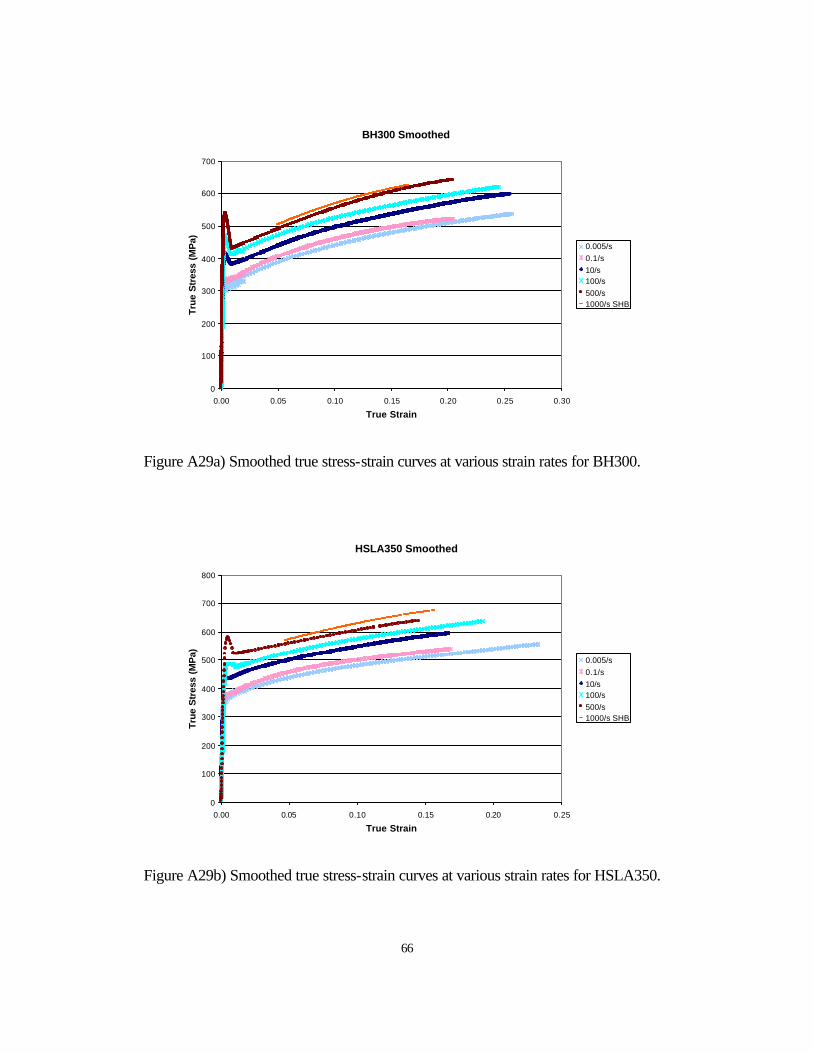
66

BH300 Smoothed

0

100

200

300

400

500

600

700

0.00 0.05 0.10 0.15 0.20 0.25 0.30

True Strain

True

Str

ess

(MP

a)

0.005/s0.1/s10/s100/s500/s1000/s SHB

Figure A29a) Smoothed true stress-strain curves at various strain rates for BH300.

HSLA350 Smoothed

0

100

200

300

400

500

600

700

800

0.00 0.05 0.10 0.15 0.20 0.25

True Strain

True

Str

ess

(MP

a)

0.005/s0.1/s10/s100/s500/s1000/s SHB

Figure A29b) Smoothed true stress-strain curves at various strain rates for HSLA350.

67

440W Smoothed

0

100

200

300

400

500

600

700

800

0.00 0.05 0.10 0.15 0.20 0.25 0.30

True Strain

True

Str

ess

(MP

a)0.005/s0.1/s10/s100/s500/s1000/s SHB

Figure A29c) Smoothed true stress-strain curves at various strain rates for 440W.

HSS590 Smoothed

0

100

200

300

400

500

600

700

800

900

1000

0.00 0.05 0.10 0.15 0.20 0.25 0.30

True Strain

True

Str

ess

(MP

a)

0.005/s0.1/s10/s100/s500/s1000/s SHB

Figure A29d) Smoothed true stress-strain curves at various strain rates for HSS590.

68

TRIP590 Smoothed

0

100

200

300

400

500

600

700

800

900

1000

0.00 0.05 0.10 0.15 0.20 0.25 0.30 0.35

True Strain

Ture

Str

ess

(MP

a)0.005/s0.1/s10/s100/s500/s1000/s SHB

Figure A29e) Smoothed true stress-strain curves at various strain rates for TRIP590.

DP600 Smoothed

0

200

400

600

800

1000

1200

0.00 0.05 0.10 0.15 0.20 0.25

True Strain

True

Str

ess

(MP

a)

0.005/s0.1/s10/s100/s500/s1000/s SHB

Figure A29f) Smoothed true stress-strain curves at various strain rates for DP600.

69

DP800 Smoothed

0

200

400

600

800

1000

1200

0.00 0.02 0.04 0.06 0.08 0.10 0.12 0.14 0.16 0.18 0.20

True Strain

True

Str

ess

(MP

a)0.005/s0.1/s10/s100/s500/s1000/s SHB

Figure A29g) Smoothed true stress-strain curves at various strain rates for DP800.

70

Table A3. True Flow Stresses at Various Strain Rates

Steel Grade

Strain Rate (1/s)

σ0.005

(MPa) σ0.02

(MPa) σ0.05

(MPa) σ0.10

(MPa) σ0.15

(MPa) σ0.20

(MPa) σ0.25

(MPa) 0.005 301 340 385 438 479 510 539 0.1 328 353 400 458 497 526 10 405 395 442 499 540 573 599 100 452 435 473 525 564 598 627 500 534 448 491 557 607 641

BH300

1000 504 569 615 645 0.005 362 399 438 479 506 531 0.1 376 411 458 499 526 10 434 464 501 547 583 100 486 480 529 574 607 634 500 582 533 560 604 638

HSLA350

1000 573 625 664 0.005 325 364 422 486 530 561 585 0.1 351 391 454 518 562 10 421 423 489 555 602 640 100 486 453 513 581 631 670 700 500 530 489 541 611 670 708

440W

1000 552 628 685 721 0.005 402 457 540 624 672 707 0.1 436 471 558 646 691 10 483 543 610 690 747 791 100 532 549 618 705 769 818 500 650 561 636 739 823 850

HSS590

1000 625 726 805 864 0.005 447 480 547 630 690 739 783 0.1 458 506 584 670 727 765 10 492 522 592 683 751 805 847 100 528 553 621 707 774 831 878 500 580 590 654 744 809 863 903

TRIP590

1000 617 708 786 850 894 0.005 437 547 628 713 765 0.1 482 584 661 736 781 10 477 595 695 783 835 874 100 506 619 720 818 876 922 500 565 681 764 843 887 930

DP600

1000 812 881 940 999 0.005 464 684 809 912 0.1 596 772 856 949 1012 10 589 765 881 985 100 703 818 906 981 1049 500 833 928 961 1023 1090

DP800

1000 983 1051 1130

71

Table A4. Tensile Properties at Various Strain Rates

Steel Grade Strain Rate (1/s)

YS (MPa)

UTS (MPa)

UE (%)

TE (%)

n-value (YS+UTS)*UE/2

(J/mm3) E10%

(J/mm3)

0.005 312 419 25.5 47.2 0.190 0.093 0.0357 0.1 337 431 18.7 34.7 0.178 0.072 0.0374 10 388 469 23.4 41.3 0.178 0.100 0.0413 100 408 490 22.7 47.5 0.148 0.102 0.0443 500 443 526 23.2 53.3 0.112 0.0463

BH300

1000 533 17.8 0.0473 0.005 352 443 19.7 41.1 0.129 0.078 0.0417 0.1 377 458 14.1 29.3 0.128 0.058 0.0422 10 429 506 15.6 33.5 0.126 0.073 0.0468 100 475 528 17.7 44.5 0.132 0.089 0.0493 500 519 554 14.9 44.4 0.080 0.0527

HSLA350

1000 577 15.7 0.0545 0.005 325 460 22.7 43.1 0.196 0.089 0.0394 0.1 350 484 16.4 31.7 0.186 0.068 0.0419 10 390 527 23.2 38.5 0.189 0.106 0.0450 100 421 548 24.4 47.5 0.180 0.118 0.0473 500 458 575 20.7 51.7 0.107 0.0504

440W

1000 592 19.3 0.0518 0.005 409 589 19.2 35.9 0.197 0.096 0.0498 0.1 440 610 14.6 27.7 0.190 0.077 0.0526 10 469 650 19.4 34.2 0.179 0.108 0.0571 100 492 683 21.2 42.6 0.195 0.124 0.0579 500 533 705 19.5 42.1 0.121 0.0596

HSS590

1000 718 19.0 0.0591 0.005 428 629 27.5 43.4 0.216 0.145 0.0507 0.1 451 637 16.6 28.8 0.190 0.090 0.0538 10 492 676 23.2 36.8 0.209 0.135 0.0549 100 525 705 25.7 45.1 0.213 0.158 0.0578 500 572 723 24.7 46.1 0.160 0.0606

TRIP590

1000 715 24.6 0.0582 0.005 417 660 14.4 34.8 0.170 0.076 0.0570 0.1 457 678 12.6 22.7 0.140 0.072 0.0611 10 498 728 18.0 27.8 0.172 0.110 0.0628 100 555 768 19.6 34.6 0.169 0.130 0.0659 500 580 777 21.9 39.7 0.149 0.0697

DP600

1000 825 20.8 0.0745 0.005 470 827 11.6 24.4 0.130 0.075 0.0740 0.1 566 872 12.0 21.8 0.135 0.086 0.0786 10 600 901 11.4 22.5 0.150 0.086 0.0807 100 678 902 15.1 29.6 0.128 0.119 0.0831 500 746 936 17.1 39.7 0.144 0.0897

DP800

1000 972 16.6 0.0900

72

5.3.3 Strain Rate Effect The yield stress and ultimate tensile stress of each steel grade are plotted versus strain rate, as shown in Figures A30 and A31. Positive strain rate sensitivity was observed for all the steel grades. Notice the strain rate sensitivity is very low at strain rates below 0.1/s, and higher when the strain rates are higher than 0.1/s, even higher for strain rates above 100/s. The change in UE and TE with strain rate is more complicated than YS and TS, as shown in Figures A32 and A33. It decreases first and then increases with minima at ~0.1/s. The UE drops again when the strain rate is higher than 100/s. While few UE and TE data are available in the literature, Rashid [A11] and Chatfield et al. [A12] showed similar behavior as observed in this study when testing mild and HSLA steels. Unfortunately, such a variation in UE data was overlooked and treated as an experimental variation. As a result, a straight line was drawn. On the other hand, Shi and Meuleman found almost no effect of strain rate on TE [A13]. The discrepency may be related to the strain rate range tested, the gage length of the specimens and the error of testing. Nevertheless, the authors believe Figures A32 truly reflects the dependence of UE on strain rate. Explanation for the dependence of UE on strain rate is attempted here. Plastic strain is mainly achieved by gliding of dislocations, which involves thermally activated motion of dislocations. For example, cross slip is often needed to overcome the barriers. At high strain rate, a thermally activated process becomes difficult due to less time available [A14]. Therefore, ductility is lower and flow stress increases at high strain rates. On the other hand, high strain rate may also delay necking and increases UE if strain rate sensitivity is higher at high strain rates. In this phenomenon, the localized necking area becomes harder and the deformation is spreading towards the neighboring areas. These two opposite processes may control the UE at different strain rates. At lower strain rates, < 0.1/s, as indicated in Figures A30 and A31, strain rate sensitivity of the tensile strength is relatively low, the effect of thermal activation is dominant, the UE decreases with increasing strain rate (Figure A32). At strain rates higher than 0.1/s, strain rate sensitivity of the tensile strength increases, suppression of necking becomes dominant, and UE increases. Note that the suppression of necking is also a time dependent process. At even higher strain rates, >100/s, the localized necking area quickly fractures due to insufficient time to deform further and to spread the strain throughout the gage section of the specimen, resulting in the drastic drop of the UE as shown in Figure A32.

73

200

300

400

500

600

700

800

900

0.001 0.01 0.1 1 10 100 1000

Strain Rate (1/s)

0.2%

Yie

ld S

tres

s (M

pa)

BH300HSLA350440WHSS590TRIP590DP600DP800

Figure A30. Yield stress vs. strain rate

200

300

400

500

600

700

800

900

1000

1100

0.001 0.01 0.1 1 10 100 1000 10000

Strain Rate (1/s)

Ten

sile

Str

ess

(Mp

a)

BH300HSLA350440WHSS590TRIP590DP600DP800

Figure A31. Ultimate tensile stress vs. strain rate

74

0

0.1

0.2

0.3

0.4

0.5

0.001 0.01 0.1 1 10 100 1000 10000

Strain Rate (1/s)

Un

ifo

rm E

lon

gat

ion

BH300HSLA350440WHSS590TRIP590DP600DP800

Figure A32. Uniform elongation vs. strain rate

0

0.1

0.2

0.3

0.4

0.5

0.6

0.001 0.01 0.1 1 10 100 1000

Strain Rate (1/s)

To

tal E

lon

gat

ion

BH300HSLA350440WHSS590TRIP590DP600DP800

Figure A33. Total elongation vs. strain rate

75

Figure A34. n-values vs. strain rate

Figure A35. Energy absorption before necking per unit volume vs. strain rate.

0

0.02

0.04

0.06

0.08

0.1

0.12

0.14

0.16

0.18

0.001 0.01 0.1 1 10 100 1000

Strain Rate, /second

(YS

+UT

S)*

UE

/2, J

/mm

3

BH300440WHSLA350HSS590DP600TRIP590DP800

0

0.05

0.1

0.15

0.2

0.25

0.001 0.01 0.1 1 10 100 1000

Strain Rate (1/s)

n V

alu

e

BH300HSLA350

440WHSS590

TRIP590DP600DP800

76

Figure A36 Energy absorption before necking per unit volume vs. strain rate for HSS590, DP600 and TRIP590 in comparison with HSLA350.

The dependence of work hardening rates of the steels on strain rate can be seen in Figure A34, where n-values are plotted against strain rate. The TRIP steel shows the highest over all n-values, around 0.2. Though the determination of n-values is subjective, especially at high strain rate, several trends can be pointed out from the plot. First, for lower strength steels, such as BH300, the n-value tends to decrease with strain rate. 440W shows the same pattern. This result is in agreement with many previous studies for lower strength steels such as IF and DQSK [A10, A12, A14]. With the increase of steel strength, the n-value becomes less dependent on the strain rate, as seen for all other five high strength steels. The decreasing strain rate sensitivity of n-value with increase steel strength was also noted by Shi et al. [A12]. The low sensitivity of n-value for higher strength steels implies that the formability of the high strength steels may not deteriorate as much as DQSK.

0

0.02

0.04

0.06

0.08

0.1

0.12

0.14

0.16

0.18

0.001 0.01 0.1 1 10 100 1000

Strain Rate, /second

(YS

+UT

S)*

UE

/2, J

/mm

3

HSLA350HSS590DP600TRIP590

77

Figure A37 Energy absorption below 10% strain in the stress-strain curve vs. strain rate

Figure A38 Energy absorption below 10% strain in the stress-strain curve vs. UTS at 10-3/s

0

0.01

0.02

0.03

0.04

0.05

0.06

0.07

0.08

0.09

0.1

0.001 0.01 0.1 1 10 100 1000 10000

Strain Rate, (1/s)

En

erg

y A

bso

rpti

on

at

10%

Str

ain

, (J/

mm

3)BH300440W

HSLA350HSS590

DP600TRIP590

DP800

BH300

440WTRIP590

HSS590

DP600

DP800

HSLA350

0

0.01

0.02

0.03

0.04

0.05

0.06

0.07

0.08

0.09

0.1

200 300 400 500 600 700 800 900

UTS at 10-3/s,MPa

E1

0% ,

J/m

m3

100/s500/s

78

Energy absorption during tests at high strain rates is an important indicator for measuring the crashworthiness of the steel. The values of [(YS+TS)/2]*UE is plotted versus strain rate for each material in Figure A35. The curves follow the same pattern as that of uniform elongation, as seen in Figure A32 since UE is one of the major contributor to the energy absorption. It is clear that the TRIP steel shows a superior energy absorption capability to the other steels within the strain rate investigated. Although its YS and UTS are lower than those of DP600, its energy absorption is the highest due to its superior UE. HSLA350 has the lowest energy absorption except at the quasi-static condition. It is also surprising to see that although DP800 has a much higher strength than other steel grades, its energy absorption is at most comparable with BH300, 440W, HSS590 and DP600 at strain rates below 100/s. Only at very high strain rates, 500/s, does DP800 exhibit higher energy absorption than the other steels, since unlike the other steels, its UE did not drop as much at 500/s as discussed. Figure A36 shows the comparison of HSS590, DP600 and TRIP590 with HSLA350 for the energy absorption. The advantage of the AHSS over the conventional HSS is evident. If the value at 100/s is used for comparison, the results show that the energy absorption for HSS590 is 51% higher than that for the HSLA350. The DP600 and TRIP590 are 81% and 100% higher, respectively. However, the E10% shows a totally different picture as shown in Figure A37. The strain rate dependence does not show any resemblance to the UE behavior. The E10% increases with increasing strain rate for all steels. In contrast to the total energy absorption before necking, DP800 exhibits the highest E10% values. In Group 2, DP600 exhibits the highest E10% value. HSS590 and TRIP590 show similar E10% , lower than DP600. TRIP590 no longer shows any advantage over DP600 and HSS590. The steels in Group 1 exhibit even lower E10% values with BH300 being the lowest. Figure A38 is a plot for E10% vs. UTS at 10-3/s for both 100/s and 500/s. The results show that E10% value is linearly dependent on the UTS of the steel in the quasi-static condition. HSS590, DP600 and TRIP590, still exhibit better energy absorption of E10% than HSLA350. However, the improvement at 100/s is reduced to 17%, 34% and 17%, respectively. Much lower than the improvements for the [(YS+TS)/2]*UE as discussed. This indicates that if only 10%, or any fixed amount of deformation is allowed in a structure during crash, the improvement of the crash performance by using the AHSS to replace the conventional HSS is less than the AHSS potentially can offer. It should be noted that stamping or other forming process could change the strength and microstructure of the steels and thus affect the energy absorption capability during further crash deformation.

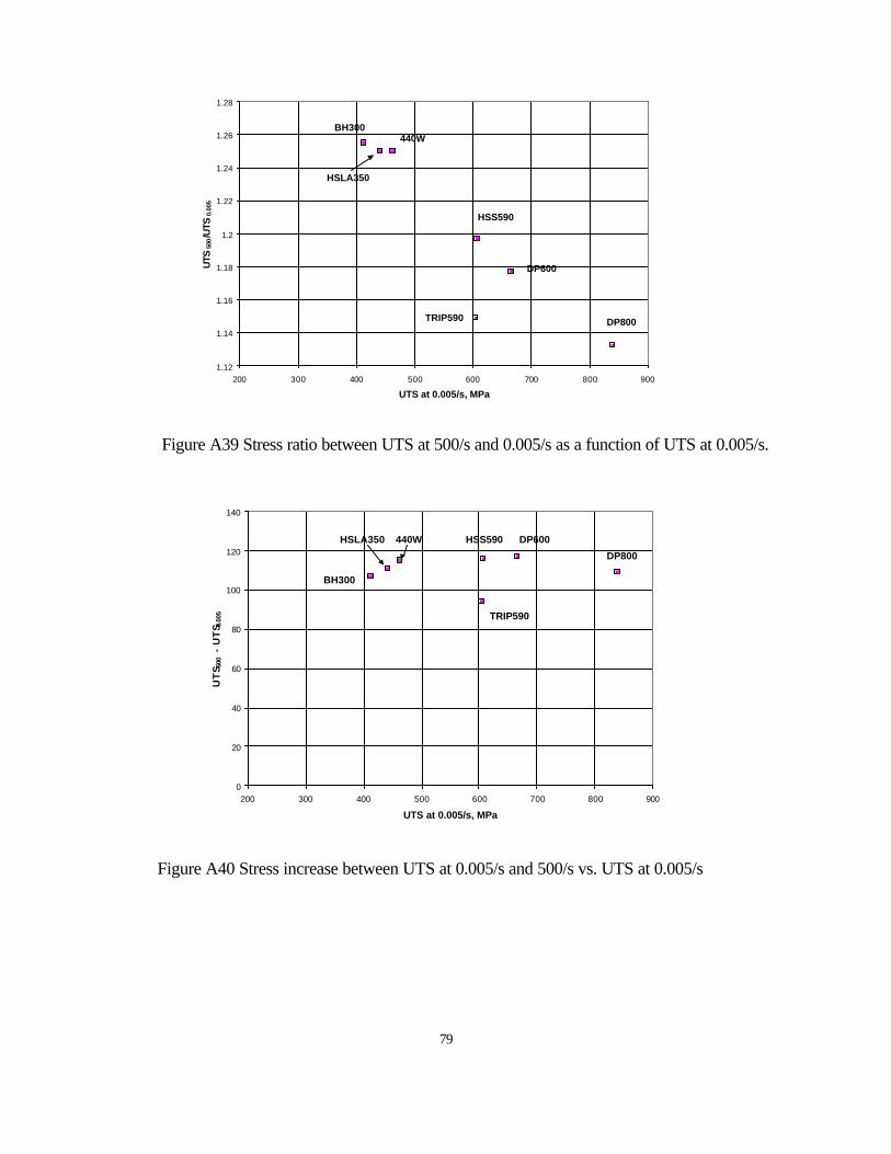
79

Figure A39 Stress ratio between UTS at 500/s and 0.005/s as a function of UTS at 0.005/s.

Figure A40 Stress increase between UTS at 0.005/s and 500/s vs. UTS at 0.005/s

1.12

1.14

1.16

1.18

1.2

1.22

1.24

1.26

1.28

200 300 400 500 600 700 800 900

UTS at 0.005/s, MPa

UTS

500/U

TS0.

005

TRIP590

BH300440W

HSLA350

HSS590

DP600

DP800

0

20

40

60

80

100

120

140

200 300 400 500 600 700 800 900

UTS at 0.005/s, MPa

UT

S 500

- U

TS 0

.005 TRIP590

BH300

440WHSLA350 HSS590 DP600

DP800

80

5.3.4 Strain Rate Sensitivity To evaluate the strain rate sensitivity of these seven different steels, the following simplified Johnson - Cook equations are used here:

+=

00 ln*1*

εε&&

YSCYSYS (9)

+=

00 ln*1*

εε&&

UTSCUTSUTS (10)

where 0ε& = 0.005 in this case, YS0 and UTS0 are the corresponding yield strength and ultimate tensile strength, respectively. CYS and CUTS are the strain rate sensitivity factor for YS and UTS, respectively. The higher the C value, the higher the strain rate sensitivity. By plotting the YS/YS0 and UTS/UTS0 as a function of ln(ε/ε0), the CYS and CUTS can be determined from the linear regression. The values are listed in Table A5. In addition, the values generated in a separate project [A16] are also given in a parenthesis for comparison. As mentioned, the measurement of YS is less accurate. Therefore, the value CYS is less reliable than the CUTS. Comparison with previous results given in the parentheses also shows much better reproducibility of the CUTS value. The following discussion on strain rate sensitivity will be based on the CUTS value only.

Table A5 CYS and CUTS for Simplified Johnson-Cook Model

Steel Grade

YS0 UTS0 CYS CUTS

BH300 312 419 0.0351 0.0225

440W 325 460 0.0336 0.0225

HSLA350 352 443 0.0467 0.0213

HSS590 409 589 0.0398 (0.0296)*

0.0154 (0.0122)

TRIP590 428 629 0.025 0.0139

DP600 448 660 0.0114 (0.0509)

0.0188 (0.0128)

DP800 547 827 0.0292 0.0117

* The data in the parentheses are from B. Yan, Reference [A16].

81

As normally believed, the strain rate sensitivity decreases with the strength of the steel. The CUTS values in Table A5 again confirm this to be true. The steels in Group 1, BH300, 440W and HSLA350, exhibit similar strain rate sensitivity, CUTS = 0.0213-0.0225. The strain rate sensitivities of the steels in Group 2, HSS590, DP600 and TRIP590, with CUTS = 0.0139-0.0188, are lower than those of steels in Group 1. And Group 3, DP800 exhibits the lowest strain rate sensitivity and the lowest CUTS value, 0.0117. In Group 2, DP600 shows slightly higher strain rate sensitivity than HSS590. TRIP590 exhibits the lowest strain rate sensitivity. This is related to the decreasing tensile strength at 1000/s as mentioned. Some researchers use the dynamic factor, the ratio of the UTS at high strain divided by the UTS at the quasi-static condition [A17, A18]. Figure A39 shows the ratio of UTS at 500/s vs. the UTS at 0.005/s as a function of the quasi-static UTS. It again shows that the strain rate sensitivity decreases with the tensile strength of the steels at the quasi-static condition. However, it should be noted that the increase of the flow stress due to the increase of strain rate does not change significantly for steels of different strength. Only the percentage increase, or the ratio, of the flow stress decreases with increasing tensile strength of the steel. Figure A40 shows the stress increase between the UTS at 500/s and 0.005/s as a function of the quasi-static UTS. It is evident while the stress ratio decreases with the increase of UTS as shown in Figure A39 the increase of UTS is around 110 MPa for all the steels tested. This translates to 22 MPa increase of UTS for each increase in order of strain rate magnitude in average. It is noticed that TRIP590 seems to have much lower strain rate sensitivity than HSS590 and DP600 as shown in Figures A39 and A40. Its CUTS value is also the lowest in Group 2. It is possible that heat generated at high strain rates may have increased the stability of the retained austenite and thus decreases UTS as demonstrated by Kanz et al. [A19]. However, more tests for TRIP steels should be conducted in order to collect more evidence. 5.4 Constitutive Model The smoothed tensile stress strain data can be fit for different constitutive models. In the last section, a simplified Johnson-Cook model was used to fit the YS or UTS only to demonstrate the strain rate sensitivity. In crash analysis, the entire stress-strain curve rather than only one or two data points should be fit to certain constitutive models. Zerilli - Armstrong (ZA) and Johnson-Cook (JC) models are popular ones for crash simulation. The former is additive and the latter is multiplicative. This means that the ZA model predicts stress-strain curves parallel to each other, whereas the JC model predicts diverging curves. However, test results can vary and often show "converging" curves, which is attributed to adiabatic heating [A20]. In order to fit the test results with more flexibility, a new modified model based on the Johnson-Cook model is developed in this study. The new model can be expressed by the following equation without the temperature term:

82

[ ]')(

ln)(1n

n

DC

CK

εε

εεεσ

=

+= & (11)

In this equation, the true stress-strain curve is simplified by a power law relation, Kεn. In contrast to the JC model, where C is a constant, the C (ε) in this model is a power function of strain ε. D and n' are the constants. Depending on the value of n', the curves can be "additive" if (n + n') = 0, "diverging" if (n + n') >0, or "converging" if (n + n') < 0. The results of fitting parameters K, n, D and n’ are listed in Table A6. All these steels showed the diverging feature, not the converging as reported by Los Alamos National Lab [A20]. Comparisons between the model prediction and actual smoothed experimental data can be seen in Figures A41a to A41g. The fit for the experimental data is reasonably good. However, the prediction is lower than the experimental data at 1000/s for all steels.

Table A6. Parameters for the New Constitutive Model

Steel Grade

K D n n’ UE CUTS = D(UE)n'

CUTS from Table 5

Ave. n from Table 4

BH300 760.6 0.0179 0.194 -0.0849 0.235 0.0202 0.0225 0.183

440W 858.2 0.0204 0.201 -0.0061 0.229 0.0206 0.0225 0.197

HSLA350 741.8 0.0254 0.141 0.0515 0.181 0.0233 0.0213 0.134

HSS590 1094.2 0.0251 0.211 0.235 0.206 0.0173 0.0154 0.198

TRIP590 1153.8 0.0127 0.226 0.0049 0.253 0.0126 0.0139 0.215

DP600 1105.2 0.0212 0.153 0.148 0.182 0.0164 0.0188 0.153

DP800 1316.8 0.0148 0.135 0.168 0.147 0.0107 0.0117 0.133

83

BH300 Model Prediction

0

100

200

300

400

500

600

700

0.00 0.05 0.10 0.15 0.20 0.25 0.30

True Strain

True

Str

ess

(MP

a)0.005/s0.1/s10/s100/s500/s1000/s SHB

Figure A41a. Comparison between the smoothed experimental data and model prediction (dashed lines) for BH300.

440W Model Prediction

0

100

200

300

400

500

600

700

800

0.00 0.05 0.10 0.15 0.20 0.25 0.30

True Strain

True

Str

ess

(MP

a)

0.005/s0.1/s10/s100/s500/s1000/s SHB

Figure A41b. Comparison between the smoothed experimental data and model prediction (dashed lines) for 440W.

84

HSLA350 Model Prediction

0

100

200

300

400

500

600

700

800

0.00 0.05 0.10 0.15 0.20 0.25 0.30

True Strain

True

Str

ess

(MP

a)0.005/s0.1/s10/s100/s500/s1000/s SHB

Figure A41c. Comparison between the smoothed experimental data and model prediction (dashed lines) for HSLA350.

HSS590 Model Prediction

0

100

200

300

400

500

600

700

800

900

1000

0.00 0.05 0.10 0.15 0.20 0.25 0.30

True Strain

True

Str

ess

(MP

a)

0.005/s0.1/s10/s100/s500/s1000/s SHB

Figure A41d. Comparison between the smoothed experimental data and model prediction (dashed lines) for HSS590.

85

DP600 Model Prediction

0

200

400

600

800

1000

1200

0.00 0.05 0.10 0.15 0.20 0.25 0.30

True Strain

True

Str

ess

(MP

a)0.005/s0.1/s10/s100/s500/s1000/s SHB

Figure A41e. Comparison between the smoothed experimental data and model prediction (dashed lines) for DP600.

TRIP590 Model Prediction

0

100

200

300

400

500

600

700

800

900

1000

0.00 0.05 0.10 0.15 0.20 0.25 0.30 0.35

True Strain

Ture

Str

ess

(MP

a)

0.005/s0.1/s10/s100/s500/s

Figure A41f. Comparison between the smoothed experimental data and model prediction (dashed lines) for TRIP590.

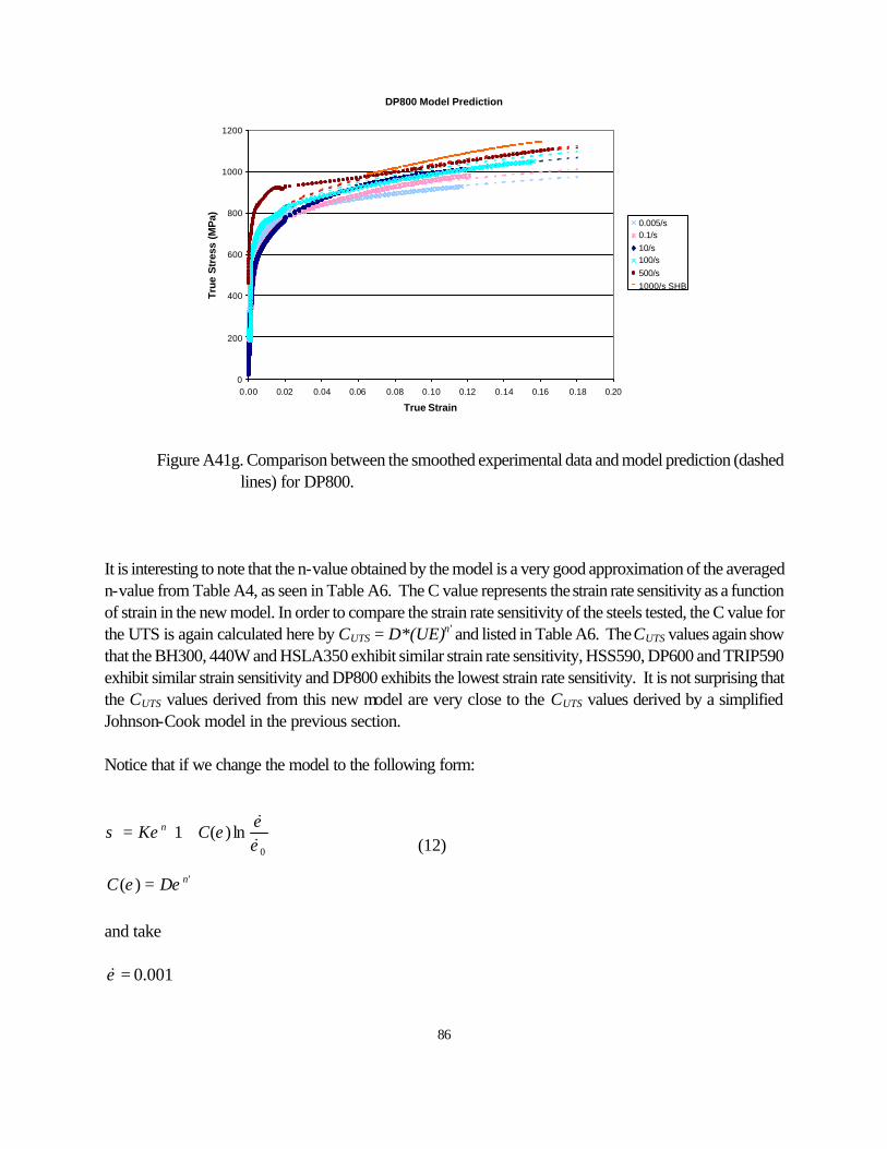
86

DP800 Model Prediction

0

200

400

600

800

1000

1200

0.00 0.02 0.04 0.06 0.08 0.10 0.12 0.14 0.16 0.18 0.20

True Strain

True

Str

ess

(MP

a) 0.005/s0.1/s10/s100/s500/s1000/s SHB

Figure A41g. Comparison between the smoothed experimental data and model prediction (dashed lines) for DP800.

It is interesting to note that the n-value obtained by the model is a very good approximation of the averaged n-value from Table A4, as seen in Table A6. The C value represents the strain rate sensitivity as a function of strain in the new model. In order to compare the strain rate sensitivity of the steels tested, the C value for the UTS is again calculated here by CUTS = D*(UE)n' and listed in Table A6. The CUTS values again show that the BH300, 440W and HSLA350 exhibit similar strain rate sensitivity, HSS590, DP600 and TRIP590 exhibit similar strain sensitivity and DP800 exhibits the lowest strain rate sensitivity. It is not surprising that the CUTS values derived from this new model are very close to the CUTS values derived by a simplified Johnson-Cook model in the previous section. Notice that if we change the model to the following form:

'

0

)(

ln)(1

n

n

DC

CK

εε

εε

εεσ

=

+=

&&

(12)

and take

001.0=ε&

87

then Kεn is the power law equation of the quasi-static stress strain curve. By estimating the D and n' values from the testing results of steels with similar strength, the stress-strain data at high strain rates for a new steel may be generated from this equation when no testing data are available. More detailed evaluation of the new constitutive model is underway and will be reported elsewhere when completed. 6. Conclusions In addition to the data generated for the six AHSS and one conventional HSS in fatigue, notch sensitivity and high strain rate, the following can be concluded from this study: Fatigue 1. In general, the steels with similar UTS exhibit similar fatigue strength. The higher the UTS, the better the

fatigue strength. For example, the steels in Group 1 with UTS between 400-440 MPa, BH300, 440W and HSLA350, exhibited similar fatigue strength. The steels in the Group 2 with UTS of 590-600 MPa, HSS590 and DP600 and TRIP590, exhibited better fatigue strength than the steels in Group 1. The steel in Group 3, DP800, exhibited even higher fatigue strength.

2. The fatigue strength of the dual phase steel, DP600, is not significantly different from HSS590. However, TRIP590 exhibited exceptionally high fatigue strength. This is believed to be the result of extra strengthening from the retained austenite to martensite transformation during cyclic deformation.

3. The AHSS exhibit a significant advantage over the conventional high strength steels. In particular, the fatigue limit of HSS590 and DP600 is 15% higher than that for HSLA350. The fatigue limit of TRIP590 is 68% higher than that of HSLA350.

4. Stress concentration as a result of a centered hole significantly reduces the fatigue strength of the steels. However, there is no significant difference in notch sensitivity for the steels studied except DP800. Therefore, the AHSS maintains its advantage over the conventional HSS, such as HSLA350 even when notches are present. The exception is DP800, which exhibits higher notch sensitivity and therefore reduced notch fatigue strength at the high cycle region.

High strain rate testing 1. The servo-hydraulic system can produce stress-strain data for a wide range of strain rates useful for

automotive crashworthiness, from quasi-static to 500/s. The stress-strain data produced by tension SHB at strain rates higher than 500/s match better with the servo-hydraulic results than the compression SHB.

2. In the servo-hydraulic tests, attaching strain gages can produce high quality strain data up to 2%. It is suggested that this method be used in combination with other methods of strain measurement, such as displacement or optical extensometer, to assure the quality of the stress-strain curves at high strain rates.

Tensile properties of the AHSS at high strain rates 1. There is no obvious change of the modulus of elasticity with strain rate in the strain rate range tested. 2. All seven steels show a positive strain rate sensitivity. However, the strain rate sensitivity, defined as the

88

percentage increase, or ratio, of flow stress due to the increase of strain rate, decreases with the strength of the steel grade. Steels in the same group exhibit the similar strain rate sensitivity. The steels in the Group 1, BH300, 440W and HSLA350, exhibit higher strain rate sensitivity than the steels in Group 2, HSS590, DP600 and TRIP590. The Group3, DP800 exhibits the lowest strain rate sensitivity. However, the increase of flow stress is almost constant for all steels tested, around 22 MPa increase of UTS for each increase of strain rate in order of magnitude in average.

3. The uniform elongation of the steels exhibits a complicated relationship with strain rate. It decreases with increasing strain rate below 0.1/s, and then increases until 100/s, where it starts to drop again. This phenomenon is attributed to the competing effect of strain rate on the thermal activation process of dislocation motion and the suppression of necking.

4. For BH300 and 440W, the full curve n-value decreases with increasing strain rate. The strain rate dependence of the n-value decreases with steel strength. HSLA350 shows very low strain rate sensitivity. The TRIP steel shows the highest work hardening rate in the strain rate range investigated.

3. Two different parameters can be used to describe the capability of steels to absorb energy in the crash event: (YS+UTS)/2*UE, representing the potential of a steel to absorb energy before necking, and E10% , the energy absorption at 10% strain, which can be used to compare crash performance of steels when a certain amount of energy absorption is required or a certain amount of deformation is allowed for a structure. Using either parameter, the AHSS exhibit better energy absorption capability than the conventional high strength steels.

5. A new constitutive model, modified from the Johnson - Cook model, has been developed. Using parameters in the model as functions of strain, the new model can become additive, multiplacative, or neither so that it can fit testing data at various strain rates which are parallel, converging or diverging. The model also has a potential to estimate high rate stress-strain data from quasi-static data when no testing results are available.

References [A1] Testing Procedures for Strain Controlled Fatigue Test (Supplement Instructions for A/SP Sheet Steel

Fatigue Program), February 1998, Auto/Steel Partnership [A2] B. Yan, P. Belanger and K. Citrin, "Effect of Forming Strain on Fatigue Performance of a Mild

Automotive Steel", SAE Publication, 2001-01-0083, 2001 [A3] H. Neuber, "Theory of Stress Concentration for Shear Strained Prismatical Bodies with Arbitrary

Nonlinear Stress-Strain Law", J. of Applied Mechanics, Dec. 1961, pp. 544-550 [A4] T.H. Topper, R.M.Wetzel, and JoDean Morrow, "Neuber's Rule Applied to Fatigue of Notched

Specimens", Journal of Materials, JMLSA, Vol. 4, No. 1, 1969, pp. 200-209 [A5] Automotive Steel Design Manual, Auto/Steel Partnership, April, 2000, p. 3.5-43 [A6] Y. Murakami, T. Nomoto, and T. Ueda, "Factors Influencing the Mechanicm of Superlong Fatigue

Failure in Steels", Fatigue Fract. Engng Mater. Struct. 22, pp. 581-590, 1999 [A7] C. Bathias, "There is No Infinite Fatigue Life in Nonmetallic Materials", Fatigue Fract. Engng Mater.

Struct. 22, pp. 559-565, 1999 [A8] P. Follansbee, “The Hopkinson Bar”, Mechanical Testing, Metals Handbook 8, ASM, p198, 1999. [A9] K. Sato, A. Yoshitake, and Y. Hosoya, "A Study on Improving the Crashworthiness of Automotive

89

Parts by using Hat Square Columns", IBEC'97, Interior, Safety & Environment, pp. 89-97, 1997 [A10] Y. Ojima, Y. Shiroi, Y. Taniguchi, and K. Kato, "Application to Body Parts of High Strength Steel

Sheet Containing Large Volumen Fraction of Retained Austenite", SAE 980954, SAE, 1998 [A11] M. S. Rashid, "Strain rate effect of mechanical behavior: a comparison between SAE 980X steels,

SAE1008 steel and 6061-T6 aluminum", Research Publication GMR-2134, 1976 [A12] D. A. Chatfield and R. R. Rote, “Strain Rate Effects on the Properties of High Strength Low Alloy

Steels”, SAE Paper No. 740177, 1974. [A13] M. Shi and D. J. Meuleman, "Strain rate sensitivity of automotive steels", SAE Technical Paper

Series, 920245, SAE, 1992. [A14] K. Xu and R. J. Arsenault, “High Temperature Deformation of NiAl Matrix Composites”, Acta

Mater., Vol. 47, No. 10, P3023, 1999. [A15] B. S. Levy, B. Yan and M. J. Stringfield, "A hardening rule for steel combining strain and strain rate

hardening and it application in stamping", 2000 IDDRG presentation, 2000. [A16] B. Yan, Ispat Inland Inc. Internal Report, July 13, 2001, Ispat Inland Inc. Research Department [A17] R. G. Davis and C. L. Magee, "The Effect of Strain Rate Upon the Tensile Deformation of

Materials", Journal of Engineering Materials and Technology, April 1975, pp. 151-155, 1975 [A18] E. Nakanishi, H. Tateno, Y. Hishida and K. Shibata, "New Materials Technology for Achieving

Both Crashworthiness and Weight reduction Using Energy Absorbing Steel with Higher Strain Rate Sensitivity", SAE 980953, SAE, 1998

[A19] S. Kantz, W. Bleck and K. Papamantellos, "The Influence of Test Temperature on the Mechanical Properties and Formability of Cold Rolled Low and High Alloyed TRIP Steels", Sheet Metal Forming Beyond 2000, Proceedings of the 20th Biennial Congress, 1998, p. 399

[A20] C. M. Cady et al, “Dynamic Materials Testing and Constitutive Modeling of Structural Sheet Steel for Automotive Applications”, Progress Report, LANL, 1995.