IRREVERSIBILITY AND HYSTERESIS FOR A

FORWARD–BACKWARD DIFFUSION EQUATION

L. C. Evans 1 M. Portilheiro 2

Department of Mathematics Department of MathematicsUniversity of California University of Texas

Berkeley, CA 94720 Austin, TX 78712

Abstract. Our intention in this paper is to publicize and extend somewhat important work

of Plotnikov [P] on the asymptotic limits of solutions of viscous regularizations of an nonlinear

diffusion PDE with a cubic nonlinearity. Since the formal limit PDE is in general ill–posed,

we expect that the limit solves instead a corresponding diffusion equation with hysteresis

effects. We employ entropy/entropy flux pairs to prove various assertions consistent with this

expectation.

1. Introduction.

Initial value problems for nonlinear diffusion PDE of the general form

(1.1) ut = ∆φ(u)

are well–posed, and well–studied, provided the flux function φ : R → R is nondecreas-ing. This paper considers instead smooth nonlinearities φ which violate this monotonicitycondition, and have rather a cubic-type structure as illustrated below.

In this case the PDE (1.1) is ill–posed forwards in time whenever u takes values inthe instable “spinodal” interval (b, a), where φ is decreasing and so (1.1) corresponds to abackward diffusion. Following Novick Cohen–Pego [NC-P] and Plotnikov [P], we replace(1.1) by the “viscous” regularization

(1.2) uεt = ∆φ(uε) + ε∆uε

t

and discuss the limit of uε as ε→ 0+.

1Supported in part by NSF Grant DMS-0070480 and by the Miller Institute for Basic Research in

Science, UC Berkeley.2Supported in part by NSF grant DMS-0074037.

1

�

�

� � �����

����

Graph of φ

We intend our paper to publicize this problem, to draw particular attention to Plotnikov[P], and to contribute some additional theoretical and numerical insights. Section 2 reviewsthe basic available estimates, including the basic “entropy” inequalities. In Section 3 wedemonstrate that if a smooth boundary develops between the stable regions as ε → 0,then the entropy inequalities force this interface to move with direction changes predictedby a hysteresis loop built from the graph of φ. The short Section 4 discusses a partialL1 estimate for uε

t . We provide in Section 5 some numerical simulations, which supportsome of the heuristics developed earlier. The appendix discusses some measure theoretictools for recording the irreversibility and hysteresis effects, and records an interesting, butunproved, formula (A.7).

Our main new contribution is the analysis of the free boundary problem in Section 3.Our discussions elsewhere are, we think, interesting but not especially definitive. As wewill see, it is remarkable that the PDE (1.2) admits the “entropy” type formulations (2.10);and it remains a fascinating problem to better exploit these to understand the limitingbehavior as ε→ 0.

Nishiura’s book [N] is a good general reference for related issues, and in particular forother sorts of reaction–diffusion PDE governed by cubic–type nonlinearities. Brokate–Sprekels [B-S] and Visintin [V1, V2] provide much more information on hysteresis phe-nomena.

To keep this on-line version of our paper short, we omit a section on some prelimminarynumerical simulations.

2. Estimates and weak convergence.2

Take U to be a smooth, bounded domain in Rn, select a time T > 0, and let ε > 0. Weturn our attention to the initial/boundary-value problem

(2.1)

uεt = ∆φ(uε) + ε∆uε

t in U × (0, T ]∂∂ν (φ(uε) + εuε

t ) = 0 on ∂U × (0, T ]uε = uε

0 on U × {t = 0},

ν denoting the unit outward normal to ∂U . The structure of this PDE is greatly clarifiedby introducing the new unknown function

(2.2) vε := φ(uε) + εuεt .

Then from (1.2) we have

(2.3){

uεt = ∆vε

vε − ε∆vε = φ(uε)in U × (0, T ],

with the Neumann boundary condition

(2.4)∂vε

∂ν= 0 on ∂U × (0, T ].

Notice that (2.2) says

(2.5) uεt =

vε − φ(uε)ε

Therefore for small ε, the time derivative uεt will be positive and large on the set {vε >

φ(uε)}, and negative and large on the set {vε < φ(uε)}. So if we imagine the function vε

to be slowly–varying, the dynamics (2.5) should drive the system onto the stable part ofthe graph of φ, where φ′ ≥ 0. As the picture shows, these heuristics suggest the emergenceof hysteresis effects in the small ε limit.

Flow of the ODE, if v varies slowly3

Remark on the regularization. A mathematical interpretation of the regularization(1.2) is this. Let A denote the operator −∆, defined for functions with Neumann boundaryconditions on ∂U . Then

Jε := (I + εA)−1

is a form of the resolvent. The Yosida approximation of A is

Aε := AJε =I − Jε

ε;

and the operator Aε is bounded, say on L2(U). According to (2.3), (2.4), we have vε =Jεφ(uε); and consequently

(2.6) uεt + Aεφ(uε) = 0.

In other words, our approximation (1.2) replaces the unbounded operator A = −∆ in theill-posed evolution (1.1) with its Yosida approximation. Assuming φ is Lipschitz continu-ous, the operator Aεφ(·) is Lipschitz as well, and so the evolution (2.6) will have a uniquesolution, give the initial data. �

The really interesting question is understanding what happens to uε and vε = Jεφ(uε),as ε→ 0.

2.1. Estimates. We assume the uniform bound

(2.5) supU|gε| ≤M

for a constant M independent of ε. Using this, we easily establish

Lemma 2.1. We have the estimates(i)

(2.6) supU×[0,T ]

|uε, vε| ≤ C1,

(ii)

(2.7)∫ T

0

∫U

|Dvε|2 + ε(uεt )

2 dxdt ≤ C2

for constants C1, C2 depending only on M , φ and n.

We next generalize estimate (2.6) as follows, closely following [NC-P] and [P]. Take

(2.8) g : R→ R to be nondecreasing,4

and set

(2.9) G(z) :=∫ z

0

g(φ(s)) ds + C

for any constant C. Thus G′(z) = g(φ(z)). If g is smooth, we compute from (2.3) that

(2.10) G(uε)t = div(g(vε)Dvε)− g′(vε)|Dvε|2 − (g(vε)− g(φ(uε)))(

vε − φ(uε)ε

).

The key observation is that the last two terms are nonnegative, and so this calculation isstrongly reminiscent of “entropy/entropy flux” calculations for dissipative approximationsto conservation laws (cf. [E]).

We obtain upon integrating

Lemma 2.2. For each smooth, nondecreasing function g,

(2.11)∫ T

0

∫U

g′(vε)|Dvε|2 + µεg dxdt ≤ C3

where

(2.12) µεg := (g(vε)− g(φ(uε)))

(vε − φ(uε)

ε

)≥ 0

and C3 is a constant depending only on M and ‖G‖L∞ .

2.2. Weak convergence. In view of these estimates, there exists a sequence εj → 0and bounded functions u, v such that

(2.13)

uεj ⇀ u weakly ∗ in L∞(U × (0, T ))vεj ⇀ v weakly ∗ in L∞(U × (0, T ))Dvεj ⇀ Dv weakly in L2(U × (0, T )).

Our main goal is understanding the relationships between u, v and the equations theysatisfy. Plotnikov [P] has deeply studied this issue, coming to the following conclusions.First, let us as illustrated introduce the three branches βi (i = 0, 1, 2) of φ−1:

�

�

�

β� �� β� �� β� ��

����

�����

5

��

�

�

���������β�

���������β0

���������β2

����

�����

Graph of the inverse functions

Theorem 2.1 ([P]). There exist three measurable functions λ0, λ1, λ2, such that for a.e.point (x, t) ∈ U × (0, T ] we have

(i) 0 ≤ λi ≤ 1 (i = 0, 1, 2)(ii)

∑2i=0 λi = 1.

(iii) Furthermore, passing as necessary to a further subsequence,

(2.14) F (uεj ) ⇀ F :=2∑

i=0

λiF (βi(v))

weakly ∗ in L∞(U × (0, T )) for each continuous function F .(iv) In addition,

(2.15) vεj , φ(uεj )→ v strongly in L2(U × (0, T )).

We call λ0, λ1, λ2 the phase fractions. The importance of assertion (2.14) is its charac-terization of the limiting behavior of the uεj . Very roughly speaking, this possibly highlyoscillating sequence takes the fraction λi of its values near the branch u = βi(v), fori = 0, 1, 2.

Next we take a smooth, nonnegative function ζ ∈ C∞c (U × [0, T ]), multiply (2.10) by ζ

and integrate by parts:

∫ T

0

∫U

−G(uε)ζt + g(vε)Dvε ·Dζ dxdy =∫ T

0

∫U

(g′(vε)|Dvε|2 + µεg)ζ dxdt.

6

Passing to limits as ε = εj → 0 and recalling (2.14), (2.15) we conclude that

(2.16) Gt − div(g(v)Dv) ≤ −g′(v)|Dv|2 in U × (0, T )

for each nondecreasing function g as above. Similarly,

(2.17) ut = ∆v in U × (0, T ).

Remark: failure of strong convergence. It is certainly possible to arrange theinitial data so that any values of the phase fractions λi (i = 0, 1, 2) can occur at a timet > 0, subject only to the constraint that their sum be one.

To see this, first fix a value A < c < B. Then select for ε > 0 an intial function gε

having the form:

uε0 :=

β0(c) on Eε0

β1(c) on Eε1

β2(c) on Eε2 ,

where Eε0 , Eε

1 , Eε2 are arbitrary measurable, disjoint sets, whose union is U . Since φ(uε

0) ≡ c,the solution of (2.1) does not depend on time: uε ≡ uε

0.Given any three nonnegative measurable functions λ0, λ1, λ2, whose sum is identically

1, we can construct the sets Eε0 , Eε

1 , Eε2 so that λ0, λ1, λ2 are the resulting phase fractions,

in the sense of Theorem 2.1. In this example the functions λi do not depend on the timevariable t, but are essentially arbitrary in the x-variables. �

3. A free boundary problem with hysteresis.

In this section we illustrate the utility of the differential inequalities (2.16) if the phasefractions λ0, λ1, λ2 have a particularly simple structure. We therefore assume that

(3.1) λ0 = 0 a.e. in U × [0, T ]

and {λ1 = 1 a.e. in V1

λ2 = 1 a.e. in V2,

where V1, V2 are two open regions in U × (0, T ), with a smooth, n-dimensional interface

Γ := V1 ∩ V2.

In other words, we are supposing that{uεj → β1(v) a.e. in V1

uεj → β2(v) a.e. in V2,7

and that there is a smooth free boundary Γ separating the two pure phase regions V1, V2.We want to deduce the behavior of u in V1, V2 and to understand as well how the

interface Γ moves. We suppose that u, v are smooth in V1, V2. For each point on Γ, let

ν = (ν1, . . . , νn, νn+1) = (ν, νn+1)

denote the unit normal in Rn+1 pointing into V1. Let u1, v1 denote the values along Γfrom within V 1 and u2, v2 the values along Γ from within V 2.

Theorem 3.1. (i) We have

(3.2){

β1(v)t = ∆v in V1

β2(v)t = ∆v in V2.(ii) Furthermore,

(3.3) v1 = v2 along Γ

and

(3.4) νn+1[u] = ν · [Dxv] along Γ,

where [·] denotes a jump across the interface. That is,

[u] := u1 − u2, [Dxu] := Dxv1 −Dxv2.

(iii) Also,

(3.5)

νn+1 = 0 if v �= A, B

νn+1 ≥ 0 if v = A

νn+1 ≤ 0 if v = B,

where we write v = v1 = v2 along Γ.

�

�

� �

A hysteresis loop8

Interpretation. According to (3.5), the interface Γ moves, which is to say that a phasetransition occurs, only if v = A or B. Furthermore, if (x0, t0) ∈ Γ, the surface moves sothat for some small ε > 0, (x0, t0 − ε) lies in phase 1 and (x0, t0 + ε) lies in phase 2 onlyif v(x0, t0) ≈ B. Likewise (x0, t0 − ε) lies in phase 2 and (x0, t0 + ε) lies in phase 1 only ifv(x0, t0) ≈ A.

We can therefore envision the phase transitions as tracing out a clockwise hysteresisloop, as illustrated. �

Proof. 1. We have

(3.6) G ={

G(β1(v)) in V1

G(β2(v)) in V2,

for each function G as above. In particular,

(3.7) u ={

β1(v) in V1

β2(v) in V2;

and so (3.2) follows from (2.18). Also, (2.18) implies

0 =∫ T

0

∫U

−uζt + Dv ·Dζ dxdt

=∫∫

V1

−β1(v)ζt + Dv ·Dζ dxdt +∫∫

V2

−β2(v)ζt + Dv ·Dζ dxdt

for each ζ ∈ C∞c . Integrating by parts and remembering (3.2), (3.7), we deduce

0 =∫

Γ

(νn+1[u]− ν · [Dxv])ζ dHn.

This identity implies the Rankine–Hugoniot relation (3.4).2. We multiply (2.17) by a nonnegative function ζ ∈ C∞c and integrate by parts, to find

0 ≥∫ T

0

∫U

−Gζt + g(v)Dv ·Dζ + g′(v)|Dv|2ζ dxdt

=∫∫

V1

−G(β1(v))ζt + g(v)Dv ·Dζ + g′(v)|Dv|2ζ dxdt

+∫∫

V2

−G(β2(v))ζt + g(v)Dv ·Dζ + g′(v)|Dv|2ζ dxdt.

We once more integrate by parts, remembering that

G′(β1(v)) = g(φ(β1(v))) = g(v), G′(β2(v)) = g(v).9

It follows that

0 ≥∫∫

V1

g(v)(b1(v)t −∆v)ζ dxdt

+∫∫

V2

g(v)(β2(v)t −∆v)ζ dxdt +∫

Γ

(νn+1[G(u)]− ν · [Dxv]g(v))ζ dHn,

and consequentlyνn+1[G(u)]− ν · [Dxv]g(v) ≤ 0 along Γ.

Substituting (3.4), we rewrite this inequality to read

νn+1([G(u)]− g(v)[u]) ≤ 0 along Γ

for each nondecreasing function g.Since G′(z) = g(φ(z)), we can recast this into the form

(3.8) νn+1

(∫ β2(v)

β1(v)

g(φ(s))− g(v) ds

)≥ 0 along Γ.

3. Clearly A ≤ v ≤ B along Γ. If A < v < B, we first take g+ to be zero on (−∞, v],positive and nondecreasing on (v,∞). Then

∫ β2(v)

β1(v)

g+(φ(s))− g+(v) ds > 0

and so νn+1 ≥ 0. Next select g− to be negative and nondecreasing on (−∞, v), zero on[v,∞). This forces ∫ β2(v)

β1(v)

g−(φ(s))− g−(v) ds < 0;

whence νn+1 ≤ 0. Consequently νn+1 = 0 if A < v < B.If v = A, we take g+ as above, to deduce νn+1 ≥ 0. Likewise, νn+1 ≤ 0 if v = B. �

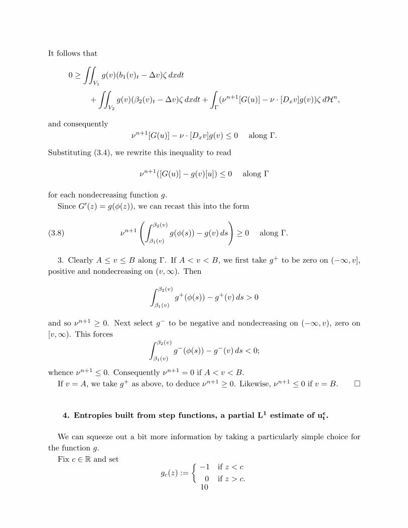
4. Entropies built from step functions, a partial L1 estimate of uεt.

We can squeeze out a bit more information by taking a particularly simple choice forthe function g.

Fix c ∈ R and set

gc(z) :={ −1 if z < c

0 if z > c.10

�

Graph of gc

�

β� �� β� �� β� ��

�����������

���������φ

Then for A < c < B, we have

G′c(z) = gc(φ(z)) =

−1 if z < β1(c)0 if β1(c) < z < β0(c)−1 if β0(c) < z < β2(c)

0 if z > β2(c).

According to (2.11), (2.12), we have∫ T

0

∫U

µεgc

dxdt ≤ C

for

µεgc

:= (gc(vε)− gc(φ(uε)))(

vε − φ(uε)ε

).

11

�

��

Recalling the definition of the step function gc, we deduce this “partial” L1 estimate onuε

t : ∫∫{(uε,vε)∈Sc}

|uεt | dxdt ≤ C,

forSc := {(x, t) |φ((uε) ≤ c ≤ vε or vε ≤ c ≤ φ((uε)}.

See the picture. Likewise ∫∫{|vε−φ(uε)|≥ε}

|uεt | dxdt ≤ C.

Remark: estimates on time derivatives. It remains an outstanding problem toimprove these L1 estimates on the time derivatives uε

t . There is some hope that suchbounds may be valid, since according to Little–Showalter [L-S] and Visintin [V1, V2],certain related hysteresis/diffusion models correspond to flows which are contractions inthe L1 norm. �

12

Appendix : Measures of irreversibility.

We introduce some measures which record certain irreversibility phenomena, and alsostate an interesting, but unproved, formula relating these measures and the time derivativesof the phase fractions.

Theorem A.1. (i) Let Φ denote an antiderivative of φ. There exist nonnegative Radonmeasures ρ, µ on U × [0, T ] such that

(A.1){ |Dvεj −Dv|2 ⇀ ρ

εj(uεj

t )2 ⇀ µ

weakly as measures. Also

(A.2) Φt − div(vDv) = −|Dv|2 − ν

in U × (0,∞), forν := ρ + µ.

(ii) For each nondecreasing C1 function g, there exist nonnegative Radon measuresρg, µg such that

(A.3)

{g′(vεj )|Dvεj −Dv|2 ⇀ ρg

µεjg := (g(vεj )− g(φ(uεj )))

(vεj−φ(uεj )

εj

)⇀ µg.

Furthermore

(A.4) Gt − div(g(v)Dv) = −g′(v)|Dv|2 − νg

in U × (0, T ), forνg := ρg + µg.

We can formally rewrite (A.2), (A.4) in the form

(A.5){

Φt − v∆v = −ν

Gt − g(v)∆v = −νg.

�

Proof. 1. According to estimate (2.7), we have

∫ T

0

∫U

|Dvε −Dv|2 + ε(uεt )

2 dxdt ≤ C

13

for some constant C1 independent of ε. Passing if necessary to a subsequence, we have(A.1). Consider next the PDE

(A.6) Φ(uε)t − div(vεDvε) = −|Dvε|2 − ε(uεt )

2.

We write−|Dvε|2 = |Dv|2 − 2Dv ·Dvε − |Dvε −Dv|2,

to see that|Dvεj |2 ⇀ |Dv|2 + ρ.

We pass to limits in (A.6) as ε = εj → 0, discovering

Φt − div(vDv) = −|Dv|2 − ρ− µ.

2. Likewise we recall the estimate (2.11) to deduce, upon passing if necessary to afurther subsequence, that (A.3) holds. The formula (A.4) results from the identity

G(uε)t − div(g(vε)Dvε) = −g′(vε)|Dvε|2 − µεg.

�

A representation formula. We record next some formal calculations using the en-tropies that suggest the following interesting, but unproved, formula. For any open set onwhich {A < v < B} and any piecewise C1, nondecreasing function g, we have

(A.7)

νg = λ1,t

∫ β0(v)

β1(v)

g(φ(r))− g(v) dr

+ λ2,t

∫ β2(v)

β0(v)

g(v)− g(φ(r)) dr

= λ1,t

∫ B

v

g′(s)(β0(s)− β1(s)) ds

+ λ2,t

∫ v

A

g′(s)(β2(s)− β0(s)) ds.

A formal derivation of (A.7) is this. According to (A.5) and (2.17),

νg = −Gt + g(v)∆v = −Gt + g(v)ut.

But

u =2∑

i=0

λiβi(v), G =2∑

i=0

λiG(βi(v));

14

and therefore

νg = −2∑

i=0

(λi,tG(βi(v)) + λi,tG′(βi(v))βi(v)t) + g(v)

2∑i=0

(λi,tβi(v) + λiβi(v)t) .

Since G′(βi(v)) = g(φ(βi(v))) = g(v), we deduce

νg =2∑

i=0

λi,t(g(v)βi(v)−G(βi(v))).

But λ0,t = −λ1,t − λ2,t, and so we can simplify the foregoing to read

νg = λ1,t[g(v)(β1(v)− β0(v))− [G(β1(v))−G(β0(v))]

+ λ2,t[g(v)(β2(v)− β0(v))− [G(β2(v))−G(β0(v))].

This expression is equivalent to (A.7).

The identity (A.7) is suggestive, in that it relates the time derivatives of the phasefractions λ1, λ2 and the dissipation measure νg, within the region {A < v < B}. But it isnot so clear to us how to make the derivation rigorous.

References

[B-S] M. Brokate and J. Sprekels, Hysteresis and Phase Transitions, Springer, 1996.

[E] L. C. Evans, Partial Differential Equations, American Math Society, third printing, 2002.

[H-L-S] U. Hornung, T. Little and R. Showalter, Parabolic PDE with hysteresis, Control Cybernet 25

(1996), 631–643.

[L-S] T. Little and R. Showalter, The super-Stefan problem, International Journal Eng. Science 33

(1995), 67–75.

[N] Y. Nishiura, Far–from–Equilibrium Dynamics; translated by K. Sakamoto, Translations of Math-

ematical Monographs 209, American Math Society, 2002.

[NC-P] A. Novick Cohen and R. Pego, Stable patterns in a viscous diffusion equation, Transactions AMS

324 (1991), 331–351.

[P] P. I. Plotnikov, Passing to the limit with respect to the viscosity in an equation with variable

parabolicity direction, Differential Equations 30 (1994), 614–622.

[V1] A. Visintin, Differential Models of Hysteresis, Springer, 1994.

[V2] A. Visintin, Forward–backward parabolic equations and hysteresis, Calculus of Variations and PDE

15 (2002), 115–132.

15