measuring the irreversibility of numerical schemes...

ESAIM: M2AN 48 (2014) 1351–1379 ESAIM: Mathematical Modelling and Numerical AnalysisDOI: 10.1051/m2an/2013142 www.esaim-m2an.org

MEASURING THE IRREVERSIBILITY OF NUMERICAL SCHEMESFOR REVERSIBLE STOCHASTIC DIFFERENTIAL EQUATIONS ∗

Markos Katsoulakis1, Yannis Pantazis

1and Luc Rey-Bellet

1

Abstract. For a stationary Markov process the detailed balance condition is equivalent to the time-reversibility of the process. For stochastic differential equations (SDE’s), the time discretization ofnumerical schemes usually destroys the time-reversibility property. Despite an extensive literature onthe numerical analysis for SDE’s, their stability properties, strong and/or weak error estimates, largedeviations and infinite-time estimates, no quantitative results are known on the lack of reversibility ofdiscrete-time approximation processes. In this paper we provide such quantitative estimates by usingthe concept of entropy production rate, inspired by ideas from non-equilibrium statistical mechanics.The entropy production rate for a stochastic process is defined as the relative entropy (per unit time)of the path measure of the process with respect to the path measure of the time-reversed process. Byconstruction the entropy production rate is nonnegative and it vanishes if and only if the process isreversible. Crucially, from a numerical point of view, the entropy production rate is an a posterioriquantity, hence it can be computed in the course of a simulation as the ergodic average of a cer-tain functional of the process (the so-called Gallavotti−Cohen (GC) action functional). We computethe entropy production for various numerical schemes such as explicit Euler−Maruyama and explicitMilstein’s for reversible SDEs with additive or multiplicative noise. In addition we analyze the entropyproduction for the BBK integrator for the Langevin equation. The order (in the time-discretizationstep Δt) of the entropy production rate provides a tool to classify numerical schemes in terms of their(discretization-induced) irreversibility. Our results show that the type of the noise critically affects thebehavior of the entropy production rate. As a striking example of our results we show that the Eulerscheme for multiplicative noise is not an adequate scheme from a reversibility point of view since itsentropy production rate does not decrease with Δt.

Mathematics Subject Classification. 65C30, 82C3, 60H10.

Received July 23, 2012. Revised September 1, 2013.Published online August 13, 2014.

1. Introduction

In molecular dynamics algorithms arising in the simulation of systems in materials science, chemical engi-neering, evolutionary games, computational statistical mechanics, etc. the steady-state statistics obtained fromnumerical simulations is of great importance [8, 27, 33]. For instance, the free energy of the system or free en-ergy differences as well dynamical transitions between metastable states are quantities which are sampled in

Keywords and phrases. Stochastic differential equations, detailed balance, reversibility, relative entropy, entropy production,numerical integration, (overdamped) Langevin process.

∗ We thanks Natesh Pillai for useful comments and suggestions. M.A.K. and Y.P. are partially supported by NSF-CMMI0835673 and L.R.-B. is partially supported by NSF -DMS-1109316.

1 Department of Mathematics and Statistics, University of Massachusetts, Amherst, MA, USA. [email protected]

Article published by EDP Sciences c© EDP Sciences, SMAI 2014

http://dx.doi.org/10.1051/m2an/2013142

http://www.esaim-m2an.org

http://www.edpsciences.org

1352 M. KATSOULAKIS ET AL.

the stationary regime. At the microscopic level, physical processes are often modeled as interactions betweenparticles described by a system of stochastic differential equations (SDE’s) [8,15]. To perform steady-state sim-ulations for the sampling of desirable observables, the solution of the system of SDE’s must possess a (unique)ergodic invariant measure. The uniqueness of the invariant measure follows from the ellipticity or hypoellipticityof the generator of the process together with irreducibility, which means that the process can reach at somepositive time any open set of the state space with positive probability [21,25]. Under such conditions, the pointdistribution of the process converges to the invariant measure (ergodicity) while the process is stationary, i.e.the distribution of the path of the process is invariant under time-shift, when the initial data are drawn from theinvariant measure. Moreover, many processes of physical origin, such as diffusion and adsorption/desorption ofinteracting particles, satisfy the condition of detailed balance (DB), or equivalently, time-reversibility, i.e., thedistribution of the path of the process is invariant under time-reversal. It is easy to see that time-reversibilityimplies stationarity but this a strictly stronger condition in general. The condition of detailed balance oftenarises from a gradient-like behavior of the dynamics or from Hamiltonian dynamics if the time-reversal includesreversal of the velocities.

However, the numerical simulation of SDE’s necessitates the use of numerical discretization schemes. Dis-cretization procedures, except in very special cases, results in the destruction of the DB condition. This affectsthe approximation process in at least two ways. First, the invariant measure of the approximation process, ifit exists at all, is not known explicitly and, second, the time reversibility of the process is lost. Several recentresults prove the existence of the invariant measure for the discrete-time approximation and provide error es-timates [2, 3, 19, 20] but, to the best of our knowledge, there is no quantitative assessment of the irreversibilityof the approximation process. Of course there exist Metropolized numerical schemes such as MALA [26] andvariations thereof [4,15] which do satisfy the DB condition but they are numerically more expensive, especiallyin high-dimensional systems, as they require an accept/reject step. Thus, a quantitative understanding of thelack of reversibility for simpler discretization schemes can provide new insights for selecting which schemes arecloser to satisfying the DB condition.

The implications of irreversibility are only partially understood, both from the physical and mathematicalpoint of view. These issues have emerged as a main theme in non-equilibrium statistical mechanics and it iswell-known that irreversibility introduces a stationary current (net flow) to the system [11,18,23,28] but it is stillunder investigation in statistical mechanics community how this current affects the long-time properties (i.e.,the dynamics and large deviations) of the process such as exit times, correlation times and phase transitions ofmetastable states. Nevertheless, a straightforward implication of irreversibility is the breaking of the symmetryof fundamental quantities and observables: for example, if a process is reversible the autocorrelation functionR(s, t) of a given observable is symmetric, i.e. R(s, t) = R(t, s). Reversibility is a natural and fundamentalproperty of physical systems and thus, if numerical approximation results in the destruction of reversibility, oneshould carefully quantify the irreversibility of the approximation process. More generally, structure preservingnumerical schemes have proved to be vastly superior (in stability) in deterministic ODE’s, e.g Stormer–Verletfor Hamiltonian systems, [10] as well as in PDE, e.g. hyperbolic conservation laws and infinite dimensionalHamiltonian systems, and there is no reason to believe it should be different in the numerical analysis ofstochastic processes. From a physical point of view the reason for detailed balance is the time-reversibility ofan underlying microscopic dynamics over which an (effective) stochastic model is presumably built. Hence,violating such a condition reduces the physical interpretation of our stochastic model. The detailed balancecondition has many implications (Kubo-formula for the linear response and Onsager relations for the responsecoefficients for example which are related to the symmetry of the autocorrelations functions) and as such itshould be preserved as much as possible in computational algorithms. In this paper we quantify irreversibilityin numerical schemes using the entropy production rate, which allows for a quantitative analysis of the pathspace statistics, including the long-time, stationary time-series regime. The entropy production rate, defined asthe relative entropy (per unit time) of the path measure of the process with respect to the path measure ofthe reversed process, is widely used in statistical mechanics for the study of non-equilibrium steady states ofirreversible systems [7, 11, 14, 18].

MEASURING THE IRREVERSIBILITY OF NUMERICAL SCHEMES 1353

A fundamental result on the structure of non-equilibrium steady states is the Gallavotti−Cohen fluctuationtheorem that describes the fluctuations (of large deviations type) of the entropy production [7, 11, 14, 18] andthis result can be viewed as a generalization of the Kubo-formula and Onsager relations far from equilibrium.Specifically for diffusion processes, entropy production governs the long time statistics of the empirical measure(also known as occupation statistics) as well as the current statistics through the Donsker–Varadhan ratefunctional, [16,17]. For our purposes, it is important to note that the entropy production rate is zero when theprocess is reversible and positive otherwise making entropy production rate a sensible quantitative measure ofirreversibility. Furthermore, if we assume ergodicity of the approximation process, the entropy production rateequals the time-average of the Gallavotti−Cohen (GC) action functional which is defined as the logarithm ofthe Radon-Nikodym derivative between the path measure of the process and the path measure of the reversedprocess. A key observation of this paper is that GC action functional is an a posteriori quantity, hence, it is easilycomputable during the simulation making the numerical computation of entropy production rate tractable. Weshow that entropy production is a computable observable that distinguishes between different numerical schemesin terms of their discretization-induced irreversibility and as such could allow us to adjust the discretization inthe course of the simulation.

We use entropy production to assess the irreversibility of various numerical schemes for reversible continuous-time processes. A simple class of reversible processes, yet of great interest, is the overdamped Langevinprocess with gradient-type drift [8, 9, 15]. The discretization of the process is performed using the explicitEuler−Maruyama (EM) scheme and we distinguish between two different cases depending on the kind of thenoise. In the case of additive noise, under the assumption of ergodicity of the approximation process [2,3,19,20]we prove that the entropy production rate is of order O(Δt2) where Δt is the time step of the numerical scheme.In the case of multiplicative noise, the results are strikingly different. Indeed, under ergodicity assumption, theentropy production rate for the explicit EM scheme is proved to have a lower positive bound which is indepen-dent of Δt. Thus irreversibility is not reduced by adjusting Δt, as the approximation process converges to thecontinuous-time process. The different behavior of entropy production depending on the kind of noise is one ofthe prominent findings of this paper. As a further step in our study, we analyze the explicit Milstein’s schemewith multiplicative noise (it is the next higher-order numerical scheme). We prove that the entropy productionrate of Milstein’s scheme decreases as time step decreases with order O(Δt).

Finally, we compute both analytically and numerically the entropy production rate for a discretization schemefor Langevin systems which is another important and widely-used class of reversible models [8,15]. The Langevinequation is time-reversible if in addition to reversing time, one reverses the sign of the velocity of all particles.The noise is degenerate but the process is hypo-elliptic and under mild conditions the Langevin equationis ergodic [20, 24, 31]. Our discretization scheme is a quasi-symplectic splitting scheme also known as BBKintegrator [5, 15]. We rigorously prove, under ergodicity assumption of the approximation process, that theentropy rate produced by the numerical scheme for the Langevin process with additive noise is of order O(Δt),hence, in terms of irreversibility it is an acceptable integration scheme.

The paper is organized in four sections. In Section 2 we recall some basic facts about reversible processesand define the entropy production. Moreover we give the basic assumptions necessary for our proofs, namely,the ergodicity of both continuous-time and discrete-time approximation process. In Section 3 we compute theentropy production rate for reversible overdamped Langevin processes. The section is split into three subsectionsfor the additive and multiplicative noise for the Euler and Milstein schemes. In Section 4 we compute the entropyproduction rate for the reversible (up to momenta flip) Langevin process using the BBK integrator. Conclusionsand future extensions of the current work are summarized in the fourth and final section.

2. Reversibility, Gallavotti−Cohen action functional, and entropy

production

Let us consider a d-dimensional system of SDE’s written as

dXt = a(Xt)dt + b(Xt)dBt (2.1)


where Xt ∈ Rd is a diffusion Markov process, a : R

d → Rd is the drift vector, b : R

d → Rd×m is the diffusion

matrix, and Bt ∈ Rm is a standard m-dimensional Brownian motion. We will always assume that a and b are

sufficiently smooth and satisfy suitable growth conditions and/or dissipativity conditions at infinity to ensurethe existence of global solutions. The generator of the diffusion process is defined by

Lf =d∑

i=1

ai∂f

∂xi+

12

d∑i,j=1

(bbT )i,j∂2f

∂xi∂xj· (2.2)

for smooth test functions f . We assume that the process Xt has a (unique) invariant measure μ(dx), and thatit satisfies the Detailed Balance (DB) condition, i.e., its generator is symmetric in the Hilbert space L2(μ):

〈Lf, g〉L2(μ) = 〈f,Lg〉L2(μ) (2.3)

for suitable smooth test functions f, g.A Markov process Xt is said to be time-reversible if for any n and sequence of times t1 < . . . < tn the finite

dimensional distributions of (Xt1 , . . . , Xtn) and of (Xtn , . . . , Xt1) are identical. More formally, let Pρ[0,t] denote

the path measure of the process Xt on the time-interval [0, t] with X0 ∼ ρ. Let Θ denote the time reversal, i.e.Θ acts on a path {Xs}0≤s≤t has

(ΘX)s = Xt−s (2.4)

Then reversibility is equivalent to Pμ[0,t] = Pμ

[0,t] ◦ Θ and it is well-known that a stationary2 process whichsatisfies the DB condition is time-reversible.

The condition of reversibility can be also expressed in terms of relative entropy as follows. Recall that fortwo probability measure π1, π2 on some measurable space, the relative entropy of π1 with respect to π2 is givenby R(π1|π2) ≡ ∫ dπ1 log dπ1

dπ2if π1 is absolutely continuous with respect to π2 and +∞ otherwise. The relative

entropy is nonnegative, R(π1|π2) ≥ 0 and R(π1|π2) = 0 if and only if π1 = π2. The entropy production rate ofa Markov process Xt is defined by

EPcont := limt→∞

1tR(Pρ

[0,t]|Pρ[0,t] ◦ Θ

)= lim

t→∞1t

∫dPρ

[0,t] logdPρ

[0,t]

dPρ[0,t] ◦ Θ

(2.5)

If Xt satisfies DB and X0 ∼ μ then R(Pμ[0,t]|Pμ

[0,t] ◦ Θ) is identically 0 for all t and the entropy productionrate is 0. Note that if X0 ∼ ρ �= μ then R(Pρ

[0,t]|Pρ[0,t] ◦ Θ) is a boundary term, in the sense that it is O(1)

and so the entropy rate vanishes in this case in the large time limit (under suitable ergodicity assumptions).Conversely when EPcont �= 0 the process is truly irreversible. The entropy production rate for Markov processesand stochastic differential equations is discussed in more detail in [14, 18].

Let us consider a numerical integration scheme for the SDE (2.1) which has the general form

xi+1 = F (xi, Δt, ΔWi) i = 1, 2, . . . (2.6)

Here xi ∈ Rd is a discrete-time continuous state-space Markov process, Δt is the time-step and ΔWi ∈ R

m, i =1, 2, . . . are i.i.d. Gaussian random variables with mean 0 and variance ΔtIm. We will assume that the Markovprocess xi has transition probabilities which are absolutely continuous with respect to Lebesgue measure witheverywhere positive densities Π(xi, xi+1) := ΠF (x,Δt,ΔW )(xi+1|xi) and we also assume that xi has a invariantmeasure which we denote μ(dx) and which is then unique and has a density with respect to Lebesgue measure.In general the invariant measure for Xt and xi differ, μ �= μ and xi does not satisfy a DB condition. Note alsothat the very existence of μ is not guaranteed in general. Results on the existence of μ do exist however andtypically require that the SDE is elliptic or hypoellitptic and that the state space of Xt is compact or that aglobal Lipschitz condition on the drift holds [2, 3, 19, 20].

2Stationarity is equivalent to starting the process Xt from its invariant measure, i.e., X0 ∼ µ.


Proceeding as in the continuous case we introduce an entropy production rate for the Markov process xi. Letus assume that the process starts from some distribution ρ(x)dx, then the finite dimensional distribution onthe time window [0, t] where t = nΔt is given by

P[0,t](dx0, . . . , dxn) = ρ(x0)Π(x0, x1) . . . Π(xn−1, xn)dx0 . . . dxn. (2.7)

For the time reversed path Θ(x0, . . . xn) = (xn, . . . , x0) we have then

P[0,t] ◦ Θ(dx0, . . . , dxn) = ρ(xn)Π(xn, xn−1) . . . Π(x1, x0)dx0 . . . dxn (2.8)

and the Radon-Nikodym derivative takes the form

dP[0,t]

dP[0,t] ◦ Θ= exp(W (t))

ρ(x0)ρ(xn)

(2.9)

where W (t) is the Gallavotti−Cohen (GC) action functional given by

W (t) = W (n; Δt) :=n−1∑i=0

logΠ(xi, xi+1)Π(xi+1, xi)

· (2.10)

Note that W (t) is an additive functional of the paths and thus if xi is ergodic, by the ergodic theorem thefollowing limit exists

EP (Δt) = limt→∞

1tW (t) = lim

n→∞1

nΔtW (n; Δt) P − a.s. (2.11)

We call the quantity EP (Δt) the entropy production rate associated to the numerical scheme. Note that wehave, almost surely,

EP (Δt) =1

Δtlim

n→∞1n

n−1∑i=0

logΠ(xi, xi+1)Π(xi+1, xi)

=1

Δt

∫ ∫μ(x)Π(x, y) log

Π(x, y)Π(y, x)

dxdy (2.12)

and for concrete numerical schemes we will compute fairly explicitly the entropy production in the next sec-tions. Since we are interested in the ergodic average we will systematically omit boundary terms which do notcontribute to ergodic averages and we will use the notation

W1(t)=W2(t) if limt→∞

1t(W1(t) − W2(t)) = 0 . (2.13)

For example we have

W (t) = logdP[0,t]

dP[0,t] ◦ Θ· (2.14)

Note also that using (2.11) and (2.10), entropy production rate is tractable numerically and it can be easilycalculated “on-the-fly” once the transition probability density function Π(·, ·) is provided.

In the following sections we investigate the behavior of the entropy production rate for different discretizationschemes of various reversible processes in the stationary regime. However, before proceeding with our analysis,let us state formally the basic assumptions necessary for our results to apply.

Assumption 2.1. We have

• The drift a and the diffusion b in (2.1) as well as the vector F in (2.6) are C∞ and all their derivatives haveat most polynomial growth at infinity.


• The generatorL is elliptic or hypo-elliptic, in particular the transition probabilities and the invariant measure(if it exists) are absolutely continuous with respect to Lebesgue with smooth densities. We assume that xt

is ergodic, i.e. every open set can be reached with positive probability starting from any point. For thediscretized scheme we assume that xi has smooth everywhere positive transition probabilities.

• Both the continuous-time process Xt and discrete-time process xi are ergodic with unique invariant measuresμ and μ, respectively. Furthermore for sufficiently small Δt we have

|Eμ[f ] − Eμ[f ]| = O(Δt) (2.15)

for functions f which are C∞ with at most polynomial growth at infinity.

Notice that inequality (2.15) is an error estimate for the invariant measures of the processes Xt and xi. Therate of convergence in terms of Δt depends on the particular numerical scheme [19, 30]. Ergodicity results for(numerical) SDEs can be found in [2, 3, 12, 19, 20, 26, 30–32]. For instance, if both drift term a(x) and diffusionterm b(x) have bounded derivatives of any order, the covariance matrix (bbT )(x) is elliptic for all x ∈ R

d andthere is a compact set outside of which holds xT a(x) < −C|x|2 for all x ∈ R

d (Lyapunov exponent) then it wasshown in [30] that the continuous-time process as well both Euler and Milstein numerical schemes are ergodic anderror estimate (2.15) holds. Another less restrictive example where ergodicity properties were proved is for SDEsystems with degenerate noise and particularly for Langevin processes [20,31]. Again, a Lyapunov functional isthe key assumption in order to handle the stochastic process at the infinity. More recently, Mattingly et al. [19]showed ergodicity for SDE-driven processes restricted on a torus as well their discretizations utilizing only theassumptions of ellipticity or hypoellipticity and the assumption of local Lipschitz continuity for both drift anddiffusion terms.

3. Entropy production for overdamped langevin processes

The overdamped Langevin process, Xt ∈ Rd, is the solution of the following system of SDE’s

dXt = −12Σ(Xt)∇V (Xt)dt +

12∇Σ(Xt)dt + σ(Xt)dBt (3.1)

where V : Rd → R is a smooth potential function, σ : Rd → R

d×m is the diffusion matrix, Σ := σσT : Rd → Rd×d

is the covariance matrix and Bt is a standard m-dimensional Brownian motion. We assume from now on thatΣ(x) is invertible for any x so that the process is elliptic. It is straightforward to show that the generator ofthe process Xt satisfies the DB condition (2.3) with invariant measure

μ(dx) =1Z

exp(−V (x))dx (3.2)

where Z =∫

Rd exp(−V (x))dx is the normalization constant and thus if X0 ∼ μ then the Markov process Xt isreversible.

The explicit Euler−Maruyama (EM) scheme for numerical integration of (3.1) is given by

xi+1 = xi − 12Σ(xi)∇V (xi)Δt +

12∇Σ(xi)Δt + σ(xi)ΔWi (3.3)

with ΔWi ∼ N(0, ΔtIm), i = 1, 2, . . . are m-dimensional iid Gaussian random variables. The process xi is adiscrete-time Markov process with transition probability density given by

Π(xi, xi+1) =1

Z(xi)exp

(1

2Δt

(Δxi +

12Σ(xi)∇V (xi)Δt − 1

2∇Σ(xi)Δt

)T

×Σ−1(xi)(

Δxi +12Σ(xi)∇V (xi)Δt − 1

2∇Σ(xi)Δt

)) (3.4)


where Δxi = xi+1 − xi and Z(xi) = (2π)m/2| det Σ(xi)|1/2 is the normalization constant for the multidi-mensional Gaussian distribution. The following lemma provides the GC action functional for the explicit EMtime-discretization scheme of the overdamped Langevin process.

Lemma 3.1. Assume that detΣ(x) �= 0 ∀x ∈ Rd. Then the GC action functional of the process xi solv-

ing (3.3) is

W (n; Δt) = − 12

n−1∑i=0

ΔxTi [∇V (xi+1) + ∇V (xi)] +

12

n−1∑i=0

ΔxTi [Σ−1(xi+1)∇Σ(xi+1) + Σ−1(xi)∇Σ(xi)]

+1

2Δt

n−1∑i=0

ΔxTi

[Σ−1(xi+1) − Σ−1(xi)

]Δxi

(3.5)

where = means equality up to boundary terms, as defined in (2.13).

Proof. The assumption for non-zero determinant is imposed so that the transition probabilities and hence theGC action functional are non-singular. The proof is then a straightforward computation using (3.4) and (2.10).

W (n; Δt) :=n−1∑i=0

[log Π(xi, xi+1) − log Π(xi+1, xi)] =n−1∑i=0

[log Z(xi+1) − log Z(xi)]

− 12Δt

n−1∑i=0

[(Δxi +

12Σ(xi)∇V (xi)Δt − 1

2∇Σ(xi)Δt

)T

×Σ−1(xi)(

Δxi +12Σ(xi)∇V (xi)Δt − 1

2∇Σ(xi)Δt

)

−(−Δxi +

12Σ(xi+1)∇V (xi+1)Δt − 1

2∇Σ(xi+1)Δt

)T

×Σ−1(xi+1)(−Δxi +

12Σ(xi+1)∇V (xi+1)Δt − 1

2∇Σ(xi+1)Δt

)]

= − 12Δt

n−1∑i=0

[ΔxT

i Σ−1(xi)Δxi +14∇V (xi)T Σ(xi)∇V (xi)Δt2 +

14∇Σ(xi)T Σ−1(xi)∇Σ(xi)Δt2

+ ΔxTi ∇V (xi)Δt − ΔxT

i Σ−1(xi)∇Σ(xi)Δt − 12∇V (xi)T∇Σ(xi)Δt2

−ΔxTi Σ−1(xi+1)Δxi− 1

4∇V (xi+1)T Σ(xi+1)∇V (xi+1)Δt2− 1

4∇Σ(xi+1)T Σ−1(xi+1)∇Σ(xi+1)Δt2

+ ΔxTi ∇V (xi+1)Δt − ΔxT

i Σ−1(xi+1)∇Σ(xi+1)Δt +12∇V (xi+1)T∇Σ(xi+1)Δt2

]

= − 12Δt

n−1∑i=0

ΔxTi

[Σ−1(xi) − Σ−1(xi+1)

]Δxi − 1

2

n−1∑i=0

ΔxTi [∇V (xi+1) + ∇V (xi)]

+12

n−1∑i=0

ΔxTi [Σ−1(xi+1)∇Σ(xi+1) + Σ−1(xi)∇Σ(xi)]

where all the terms of the general form G(xi)−G(xi+1) in the sums were cancelled out since they form telescopicsums which become boundary terms. �

Three important remarks can readily be made from the above computation.


Remark 3.2. The numerical computation of entropy production rate as the time-average of the GC actionfunctional on the path space (i.e., based on (2.9)) at first sight seems computationally intractable due to the largedimension of the path space. However, due to ergodicity, the numerical computation of the entropy productioncan be performed as a time-average based on (2.11) and (3.5) for large n. Additionally, this computation canbe done for free and “on-the-fly” since the quantities involved are already computed in the simulation of theprocess. The numerical entropy production rate shown in the following figures is computed using this approach.

Remark 3.3. It was shown in [18] that the GC action functional of the continuous-time process driven by (3.1)equals the Stratonovich integral

Wcont(t) = −∫ t

0

∇V (Xs) ◦ dXs = V (x0) − V (xt) (3.6)

which reduces to a boundary term as expected. This functional has the discretization

Wcont(t) ≈ 12

n−1∑i=0

ΔxTi [∇V (xi+1) + ∇V (xi)] (3.7)

and this is exactly the first term in the GC action functional W (n; Δt) for the explicit EM approximation process(see (3.5)). However, the discretization scheme introduces two additional terms to the GC action functionalwhich may greatly affect the asymptotic behavior of entropy production as Δt goes to zero, as we demonstratein Section 3.2. Notice that when the noise is additive, i.e., when the diffusion matrix is constant, then these twoadditional terms vanish and taking the limit Δt → 0, the GC action functional W (n; Δt), if exists, becomes theStratonovich integral Wcont(t) which is a boundary term.

Remark 3.4. The GC action functional W (n; Δt) consists of three terms (see (3.5)), each of which stems froma particular term in the SDE. Thus, each term in the SDE contributes to the entropy production functionala component which is totally decoupled from the other terms. The reason for this decomposition lies in theparticular form of the transition probabilities for the explicit EM scheme which are exponentials with quadraticargument. This feature can be exploited for the study of entropy production of numerical schemes for processeswith irreversible dynamics. Indeed, if a non-gradient term of the form a(Xt)dt is added to the drift of (3.1), theprocess is irreversible and its GC action functional is not anymore a boundary term and is given by [18]

Wcont(t)= −∫ t

0

Σ−1(Xt)a(Xt) ◦ dXt ≈ 12

n−1∑i=0

ΔxTi

[Σ−1(xi)a(xi) + Σ−1(xi+1)a(xi+1)

](3.8)

On the other hand, due to the separation property of the explicit EM scheme, the GC action functional of thediscrete-time approximation process W (n; Δt) has the additional term

12

n−1∑i=0

ΔxTi [Σ−1(xi)a(xi) + Σ−1(xi+1)a(xi+1)]. (3.9)

Evidently, the discretization of Wcont(t) equals the additional term of the GC functional W (n; Δt). Thus, theGC action functional W (n; Δt) is decomposed into two components, one stemming from the irreversibility ofthe continuous-time process and another one stemming from the irreversibility of the discretization procedure.

3.1. Entropy production for the additive noise case

An important special case of (3.1) is the case of additive noise, i.e., when the covariance matrix does notdepend in the process, Σ(x) ≡ Σ. In this case, the SDE system becomes

dXt = −12Σ∇V (Xt)dt + σdBt

X0 ∼ μ(3.10)


and the GC action functional is simply given by

W (n; Δt)= − 12

n−1∑i=0

ΔxTi [∇V (xi+1) + ∇V (xi)] (3.11)

In this section we prove an upper bound for the entropy production of the explicit EM scheme. The proofuses several lemmas stated and proved in Appendix A.

Theorem 3.5. Let Assumption 2.1 hold. Assume also that the potential function V has bounded fifth-orderderivative and that the covariance matrix Σ is invertible. Then, for sufficiently small Δt, there exists C =C(V, Σ) > 0 such that

EP (Δt) ≤ CΔt2 (3.12)

Proof. Utilizing the generalized trapezoidal rule (A.1) for k = 3, the GC action function is rewritten as

W (n; Δt)= − 12

n−1∑i=0

ΔxTi [∇V (xi+1) + ∇V (xi)]

=n−1∑i=0

⎧⎨⎩−(V (xi+1) − V (xi)) +

∑|α|=3

Cα[DαV (xi+1) + DαV (xi)]Δxαi

+∑

|α|=1,3,5

∑|β|=5−|α|

Bβ [Rβα(xi, xi+1) + Rβ

α(xi+1, xi)]Δxα+βi

⎫⎬⎭

=n−1∑i=0

∑|α|=3


+n−1∑i=0

∑|α|=1,3,5

∑|β|=5−|α|

Bβ [Rβα(xi, xi+1) + Rβ

α(xi+1, xi)]Δxα+βi .

(3.13)

Applying, once again, Taylor series expansion to DαV (xi+1), the GC action functional becomes

W (n; Δt)=n−1∑i=0

⎧⎨⎩∑|α|=3

2CαDαV (xi)Δxαi +

∑|α|=3

Cα

∑|β|=1

Dα+βV (xi)Δxα+βi

⎫⎬⎭

+n−1∑i=0

∑|α|=1,3,5

∑|β|=5−|α|

Rβα(xi, xi+1)Δxα+β

i

(3.14)

where Rβα(xi, xi+1) = Bβ [Rβ

α(xi, xi+1)+Rβα(xi+1, xi)]+�|α|=3R

αβ (xi, xi+1). Moreover, expanding Δxα

i using themulti-binomial formula

Δxαi =(−1

2Σ∇V (xi)Δt + σΔWi

)α

=∑ν≤α

(α

ν

)(−1

2Σ∇V (xi)Δt

)ν

(σΔWi)α−ν . (3.15)


Then, the GC action functional becomes

W (n; Δt) = 2n−1∑i=0

∑|α|=3

∑ν≤α

Cα

(α

ν

)DαV (xi)

(−1

2Σ∇V (xi)Δt

)ν

(σΔWi)α−ν

+n−1∑i=0

∑|α|=3

∑|β|=1

∑ν≤α+β

Cα

(α + β

ν

)Dα+βV (xi)

(−1

2Σ∇V (xi)Δt

)ν

(σΔWi)α+β−ν

+n−1∑i=0

∑|α|=1,3,5

∑|β|=5−|α|

∑ν≤α+β

(α + β

ν

)Rβ

α(xi, xi+1)(−1

2Σ∇V (xi)Δt

)ν

(σΔWi)α+β−ν .

(3.16)

From (2.11), the entropy production rate is the time-averaged GC action functional as n → ∞. Thus,

EP (Δt) = limn→∞

W (n; Δt)nΔt

=2

Δt

∑|α|=3

∑ν≤α

Cα

(α

ν

)lim

n→∞1n

n−1∑i=0

DαV (xi)(−1

2Σ∇V (xi)Δt

)ν

(σΔWi)α−ν

+1

Δt

∑|α|=3

∑|β|=1

∑ν≤α+β

Cα

(α + β

ν

)lim

n→∞1n

n−1∑i=0

Dα+βV (xi)(−1

2Σ∇V (xi)Δt

)ν

(σΔWi)α+β−ν

+1

Δt

∑|α|=1,3,5

∑|β|=5−|α|

∑ν≤α+β

(α + β

ν

)lim

n→∞1n

n−1∑i=0

Rβα(xi, xi+1)

(−1

2Σ∇V (xi)Δt

)ν

(σΔWi)α+β−ν .

(3.17)The ergodicity of xi as well the Gaussianity of ΔWi guarantees that the first two limits in the entropy productionformula exist. Additionally, the residual terms, Rβ

α(xi, xi+1), are bounded due to the assumption on boundedfifth-order derivative of V , hence, the third limit also exists. Note here that this assumption could be changed byassuming boundedness of a higher order derivative and performing a higher-order Taylor expansion. Appendix Agives rigorous proofs of these ergodicity statements. Hence,

EP (Δt) =2

Δt

∑|α|=3

∑ν≤α

Cα

(α

ν

)Eμ

[DαV (x)

(−1

2Σ∇V (x)Δt

)ν]Eρ

[(σy)α−ν

]

+1

Δt

∑|α|=3

∑|β|=1

∑ν≤α+β

Cα

(α + β

ν

)Eμ

[Dα+βV (x)

(−1

2Σ∇V (x)Δt

)ν]Eρ

[(σy)α+β−ν

]

+1

Δt

∑|α|=1,3,5

∑|β|=5−|α|

∑ν≤α+β

(α + β

ν

)Eμ×ρ

[Rβ

α(x, y)(−1

2Σ∇V (x)Δt

)ν]Eρ[(σy)α+β−ν ]

(3.18)

where μ is the equilibrium measure for xi while ρ is the Gaussian measure of ΔWi. Using the Isserlis−Wickformula we can compute the higher moments of multivariate Gaussian random variable from the second-ordermoments. Indeed, we have

E [yν ] = E [yν11 . . . yνd

d ] = E[z1z2 . . . z|ν|

]={

0 if |ν| odd∑∏E [zizj ] if |ν| even (3.19)

where∑∏

means summing over all distinct ways of partitioning z1, . . . , z|ν| into pairs. Moreover, E[zizj ] =ΣijΔt, hence, applying (3.19) into (3.18) and changing the multi-index notation to the usual notation, the


entropy production rate becomes

EP (Δt) =2

Δt

d∑k1=1

d∑k2=1

d∑k3=1

Ck1k2k3

{Eμ

[∂3V

∂xk1∂xk2∂xk3

(−1

2Σ∇V

)k1

]Σk2k3Δt2

+Eμ

[∂3V

∂xk1∂xk2∂xk3

(−1

2Σ∇V

)k2

]Σk1k3Δt2

+Eμ

[∂3V

∂xk1∂xk2∂xk3

(−1

2Σ∇V

)k3

]Σk1k2Δt2 + O

(Δt3)}

+1

Δt

d∑k1=1

d∑k2=1

d∑k3=1

d∑k4=1

Ck1k2k3

{Eμ

[∂4V

∂xk1 . . . ∂xk4

]

× [Σk1k2Σk3k4 + Σk1k3Σk2k4 + Σk1k4Σk2k3 ] Δt2 + O(Δt3)}

+1

ΔtO(Δt3).

(3.20)

Using that (− 12Σ∇V )ki = − 1

2

∑dk4=1 Σkik4

∂V∂xk4

, entropy production is rewritten as

EP (Δt) =d∑

k1=1

d∑k2=1

d∑k3=1

d∑k4=1

Ck1k2k3

{Σk1k2Σk3k4

(−Eμ

[∂3V

∂xk1∂xk3∂xk4

∂V

∂xk2

]+ Eμ

[∂4V

∂xk1 . . . ∂xk4

])

+ Σk1k3Σk2k4

(−Eμ

[∂3V

∂xk1∂xk2∂xk4

∂V

∂xk3

]+ Eμ

[∂4V

∂xk1 . . . ∂xk4

])

+Σk1k4Σk2k3

(−Eμ

[∂3V

∂xk1∂xk2∂xk3

∂V

∂xk4

]+ Eμ

[∂4V

∂xk1 . . . ∂xk4

])}Δt + O

(Δt2).

(3.21)By a simple integration by parts, we observe that for any combination k1, . . . , k4 = 1, . . . , d

Eμ

[∂3V

∂xk1∂xk2∂xk3

∂V

∂xk4

]= Eμ

[∂4V

∂xk1 . . . ∂xk4

](3.22)

where the expectation is taken with respect of μ which is the invariant measure of the continuous-time process.However, in (3.21) the expectation is w.r.t. the invariant measure of the discrete-time process (i.e., μ instead ofμ). Nevertheless, Assumption 2.1 guarantees that the alternation of the measure from μ to μ costs an error oforder O(Δt). Hence, for any coefficient in (3.21), we obtain that∣∣∣∣Eμ

[∂3V

∂xk1∂xk2∂xk3

∂V

∂xk4

]− Eμ

[∂4V

∂xk1 . . . ∂xk4

]∣∣∣∣ ≤ 2KΔt (3.23)

since the potential V as well its derivatives are sufficiently smooth. Hence, we overall showed that

EP (Δt) = O(Δt2)

(3.24)

which completes the proof. �Remark 3.6. Depending on the potential function the entropy production could be even smaller. For instance,when the potential V is a quadratic function (i.e. the continuous-time process is an Ornstein−Uhlenbeck pro-cess), then, it is easily checked by a trivial calculation of (3.11) that the GC action function is a boundary term,thus, the entropy production of the explicit EM scheme is zero. However, for a generic potential V we expectthat the entropy production rate decays quadratically as a function of Δt but not faster.


0 1 2 3 4 5 6 7 8 9 10

x 104

−15

−10

−5

0

5

10

15

Time

GC

Act

ion

Fun

ctio

nal

0 1 2 3 4 5 6 7 8 9 10

x 104

−10

−5

0

5x 10

−3

Time

Ent

ropy

Pro

duct

ion

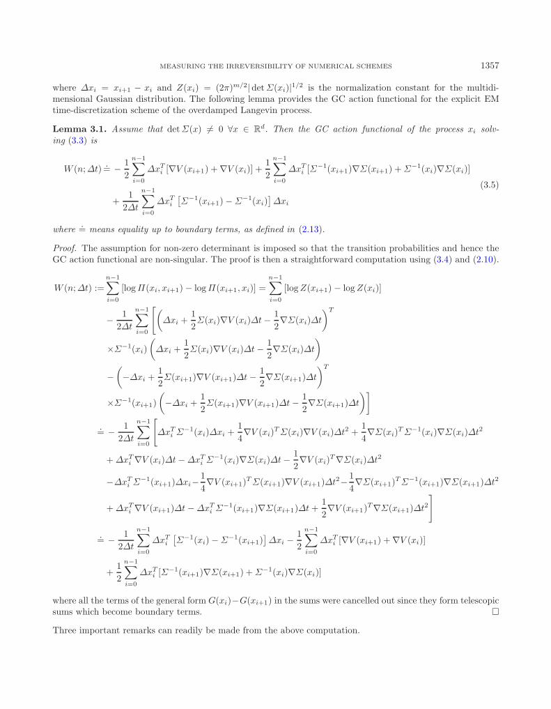
Figure 1. Upper panel: the GC action functional as a function of time for fixed Δt = 0.05. Itsvariance is large necessitating the use of many samples in order to obtain statistically confidentquantities. Lower Panel: the entropy production rate as a function of time for the same Δt. Itconverges to a positive value as expected.

3.1.1. Fourth-order potential on a torus

Lets now proceed with an important example where the potential is a forth-order polynomial while theprocess takes values on a torus. Assume d = 2 while potential V = Vβ is given by

Vβ(x) = β

( |x|44

− |x|22

)(3.25)

where β is a positive real number which in statistical mechanics has the meaning of the inverse temperature.The diffusion matrix is set to σ =

√2β−1Id. Based on [20], Assumption 2.1 is satisfied because the domain is

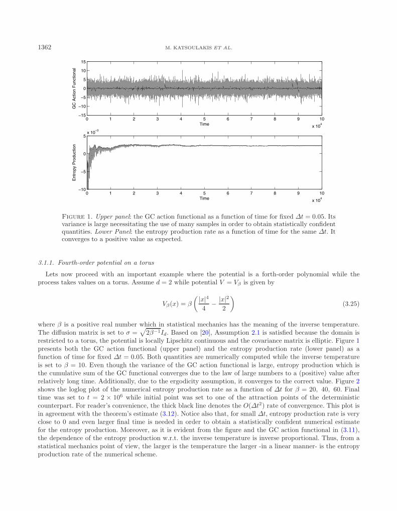
restricted to a torus, the potential is locally Lipschitz continuous and the covariance matrix is elliptic. Figure 1presents both the GC action functional (upper panel) and the entropy production rate (lower panel) as afunction of time for fixed Δt = 0.05. Both quantities are numerically computed while the inverse temperatureis set to β = 10. Even though the variance of the GC action functional is large, entropy production which isthe cumulative sum of the GC functional converges due to the law of large numbers to a (positive) value afterrelatively long time. Additionally, due to the ergodicity assumption, it converges to the correct value. Figure 2shows the loglog plot of the numerical entropy production rate as a function of Δt for β = 20, 40, 60. Finaltime was set to t = 2 × 106 while initial point was set to one of the attraction points of the deterministiccounterpart. For reader’s convenience, the thick black line denotes the O(Δt2) rate of convergence. This plot isin agreement with the theorem’s estimate (3.12). Notice also that, for small Δt, entropy production rate is veryclose to 0 and even larger final time is needed in order to obtain a statistically confident numerical estimatefor the entropy production. Moreover, as it is evident from the figure and the GC action functional in (3.11),the dependence of the entropy production w.r.t. the inverse temperature is inverse proportional. Thus, from astatistical mechanics point of view, the larger is the temperature the larger -in a linear manner- is the entropyproduction rate of the numerical scheme.


10−2

10−1

10−6

10−5

10−4

10−3

10−2

10−1

100

Δ t

Ent

ropy

Pro

duct

ion

β=20β=40β=60

Figure 2. Entropy production rate as a function of time step Δt for additive noise. Theentropy production rate is of order O(Δt2) for small Δt while it decreases linearly as a functionof inverse temperature β.

3.2. Entropy production for the multiplicative noise case: Euler−Marayuma scheme

In this section we consider the EM scheme for overdamped Langevin processes with multiplicative noise. Forsimplicity we restrict our discussion to the one dimensional case, but our results extend immediately to higherdimension if the the diffusion matrix σ(x) is diagonal. We rewrite the GC action function given in Lemma 3.1,

W (n; Δt)= − 12

n−1∑i=0

[V ′(xi+1) + V ′(xi)]Δxi +12

n−1∑i=0

[Σ−1(xi+1)Σ′(xi+1) + Σ−1(xi)Σ′(xi)]Δxi

+1

2Δt

n−1∑i=0

[Σ−1(xi+1) − Σ−1(xi)

]Δx2

i

=: W1(n; Δt) + W2(n; Δt) + W3(n; Δt).

(3.26)

The first term W1(n; Δt) has been computed in the previous section and after an interesting and rather unex-pected cancellation it was proved to be of order O(Δt2). For the multiplicative case, a cancellation also occurs(see (3.30) and (3.31) below) but it does not fully eliminate the lower order term; in the end W1(n; Δt) con-tributes to the entropy production an O(Δt) term. Additionally, W2(n; Δt) turns out to be the sum of gradientterms since Σ−1(x)Σ′(x) = (log Σ(x))′. Thus, assuming a suitable condition on Σ(x), the same computationas for W1(n; Δt) applies and the entropy production rate stemming from W2(n; Δt) is also of order O(Δt).However, W3(n; Δt) contributes to the entropy production a nonzero, positive term which is of order O(1).The following theorem summarizes the behavior of entropy production rate for the explicit EM scheme formultiplicative noise.

Theorem 3.7. Let Assumption 2.1 hold and assume that the potential function V has a bounded fifth-orderderivative, while there exists M > 0 such that Σ(x) > M−1 for all x.

(a) If c := 34Eμ[(Σ−1)(x)(Σ′)2(x)], then, for sufficiently small Δt, there exists C = C(V, Σ) > 0 independent

of Δt such that|EP (Δt) − c| ≤ CΔt (3.27)


(b) Assuming that Eμ[(Σ−1)(x)(Σ′)2(x)] �= 0, then, for sufficiently small Δt, there exists a lower bound c′ =c′(V, Σ) > 0 independent of Δt such that

c′ ≤ EP (Δt) (3.28)

Proof. The assumption that Σ(x) > M−1 ∀x, which is the ellipticity condition in one space dimension, isnecessary because it implies that Σ−1(x) as well its derivatives are bounded around 0. Additionally, as discussedearlier both W1(n; Δt) and W2(n; Δt) contribute to the entropy production by a O(Δt) amount. Therefore wecan concentrate on the term W3(n; Δt); after a Taylor series expansion we have,

W3(n; Δt) =1

2Δt

n−1∑i=0

[(Σ−1)′

(xi)Δx3i +

12(Σ−1)′′(xi)Δx4

i

+1

2Δt

n−1∑i=0

∫ 1

0

(1 − t)(Σ−1)′′′(txi+1 + (1 − t)xi)dtΔx5i

]

=1

2Δt

n−1∑i=0

3∑k=0

(3k

)(Σ−1)′(xi)

(−1

2Σ(xi)V ′(xi)Δt +

12Σ′(xi)Δt

)k

(σ(xi)ΔWi)3−k

+1

4Δt

n−1∑i=0

4∑k=0

(4k

)(Σ−1)′′(xi)

(−1


12Σ′(xi)Δt

)k

(σ(xi)ΔWi)4−k

+1

2Δt

n−1∑i=0

5∑k=0

(5k

)∫ 1

0

(1 − t)(Σ−1)′′′ (txi+1 + (1 − t)xi) dt

×(−1


12Σ′(xi)Δt

)k

(σ(xi)ΔWi)5−k.

As in Theorem 3.5, applying the ergodic lemmas of the appendix, the entropy production rate stemming fromW3(n; Δt) equals to

EP3(Δt) = limt→∞

W3(n; Δt)nΔt

=1

2Δt2

3∑k=0

(3k

)Eμ

[(Σ−1)′(x)(−1

2Σ(x)V ′(x)Δt +

12Σ′(x)Δt)kσ(x)3−k

]Eρ[ΔW 3−k]

+1

4Δt2

4∑k=0

(4k

)Eμ

[(Σ−1)′′(x)(−1

2Σ(x)V ′(x)Δt +


]Eρ[ΔW 4−k]

+1

2Δt2

5∑k=0

Eμ×ρ

[R(x, y)(−1

2Σ(x)V ′(x)Δt +


]Eρ[ΔW 5−k]

=1

2Δt2

[−3

2Eμ[(Σ−1)′(x)Σ2(x)V ′(x)]Δt2 +

32

Eμ[(Σ−1)′(x)Σ′(x)Σ(x)]Δt2 + O(Δt3)]

+1

4Δt2[Eμ

[(Σ−1)′′(x)Σ2(x)

]3Δt2 + O

(Δt3)]

+1

2Δt2O(Δt3)

=34

[−Eμ

[(Σ−1)′(x)Σ2(x)V ′(x)

]+

12

Eμ[(Σ−1)′(x)(Σ2)′(x)] + Eμ[(Σ−1)′′(x)Σ2(x)]]

+ O(Δt)

(3.29)On the other hand,

Eμ[(Σ−1)′(x)Σ2(x)V ′(x)] = Eμ[(Σ−1)′′(x)Σ2(x)] + Eμ[(Σ−1)′(x)(Σ2)′(x)] (3.30)


10−2

10−1

10−2

10−1

100

Δ t

Ent

ropy

Pro

duct

ion

(Eul

er−

Mar

uyam

a)

ε=2ε=1ε=0.5

Figure 3. Entropy production rate as a function of time step Δt for multiplicative noise andthe explicit EM scheme. As Theorem 3.7 asserts, entropy production does not decrease as Δtis decreased. This results in a permanent loss of reversibility which cannot be fixed by reducingthe time step. Star symbols denote the theoretical value of the lower bound as it is given bythe Theorem (i.e., c′ ≈ c = 3

4Eμ[(Σε)−1(x)(Σ′ε)

2(x)]). The agreement between the theoreticaland the numerical values is excellent.

Using (2.15) in Assumption 2.1 we obtain, as in the additive case, that

EP3(Δt) − 34

Eμ[(Σ−1)(x)(Σ′)2(x)] = O(Δt) (3.31)

which concludes the proof of (a). Part (b) is a direct consequence of (a). �

3.2.1. Example: quadratic potential on R

Let the quadratic potential V (x) = x2

2 , and the diffusion term

σε(x) =

√1

1 + εx2· (3.32)

The choice of the diffusion term is justified by the fact that we can control its variation in terms of x, while sendingε to zero, the additive noise case is recovered. The invariant measure of this process is the Gaussian measurewith zero mean and variance one. Moreover, all the assumptions of Theorem 3.7 are satisfied thus we expecta O(1) behavior of the entropy production rate at least for small Δt. Indeed, Figure 3 shows the numerically-computed entropy production as a function of Δt, which clearly does not decrease to zero as Δt tends to zero.Consequently, the explicit EM scheme for the multiplicative noise case totally destroys the reversibility propertyof the discrete-time approximation process independently of how small time-step is selected. Additionally, noticethat as ε decreases, entropy production also decreases. This behavior is expected since σ(x) → σ = constant asε → 0 and in combination with the quadratic potential V , EP (Δt) → 0 as ε → 0 for any Δt sufficiently small.


3.3. Entropy production for the multiplicative noise case: Milstein scheme

Since the EM scheme has entropy production rate which does not decrease as Δt decreases, we turn ourattention to the Milstein’s scheme which is the next higher-order scheme [13,22]:

xi+1 = xi − 12Σ(xi)V ′(xi)Δt +

12Σ′(xi)Δt + σ(xi)ΔWi +

12σ(xi)σ′(xi)(ΔW 2

i − Δt), (3.33)

which can be rewritten asΔxi = a(xi)Δt + σ(xi)ΔWi +

14Σ′(xi)ΔW 2

i , (3.34)

where a(xi) = − 12Σ(xi)V ′(xi)+ 1

4Σ′(xi). Since ΔWi is a zero-mean Gaussian random variable with variance Δt,the transition probability for Milstein’s scheme is

Π(xi, xi+1) =1

|√2πΔtZ(xi, Δxi)|

⎡⎣exp

⎛⎝− 1

2Δt

∣∣∣∣∣−σ(xi) +√

Z(xi, Δxi)12Σ′(xi)

∣∣∣∣∣2⎞⎠

+ exp

⎛⎝− 1

2Δt

∣∣∣∣∣σ(xi) +√


∣∣∣∣∣2⎞⎠⎤⎦

(3.35)

whereZ(xi, Δxi) = Σ(xi) + Σ′(xi) (Δxi − a(xi)Δt) . (3.36)

Notice also that Z(xi, Δxi) = (σ(xi) + 12Σ′(xi)ΔWi)2 ≥ 0 which is positive almost surely. Moreover, the

arguments of the exponentials in (3.35) are of different order in terms of Δt. Indeed, it is straightforwardto show that for small time step, Δt, the argument of the first exponential in (3.35) is of order O(1) whilethe argument of the second exponential is of order O( 1

Δt ). Thus, as Δt tends to zero, the second exponentialbecomes exponentially small and the dominating term is the first exponential. Therefore, using the fact thatlog(e−a + e−b/Δt

)= −a + O(e−b/Δt) for positive a and b, the GC action functional for Milstein’s scheme

reduces to

W (n; Δt) = − 12

n−1∑i=0

logZ(xi, Δxi)

Z(xi+1,−Δxi)

− 2Δt

n−1∑i=0

⎡⎣(−σ(xi) +

√Z(xi, Δxi)

12Σ′(xi)

)2

−(−σ(xi+1) +

√Z(xi+1,−Δxi)

12Σ′(xi+1)

)2⎤⎦

=W1(n; Δt) + W2(n; Δt)

(3.37)

where Z(xi+1,−Δxi) = Σ(xi+1)+Σ′(xi+1) (−Δxi − a(xi+1)Δt). The following theorem demonstrates that theentropy production of the Milstein Scheme is at least linear in Δt:

Theorem 3.8. Under the assumptions of Theorem 3.7 and for sufficiently small Δt, there exists C =C(V, Σ) > 0 independent of Δt such that

EP (Δt) ≤ CΔt (3.38)

Proof. In order to compute the detailed asymptotics for W1(n; Δt) and W2(n; Δt) we write the partition functionZ(xi, Δxi) as

Z(xi, Δxi) = Σ(xi) + Σ′(xi) (Δxi − a(xi)Δt)

= Σ(xi+1) −(

12Σ′′(xi)Δx2

i +16Σ′′′(xi)Δx3

i + Σ′(xi)a(xi)Δt

)+ O(Δx4

i

).

(3.39)


Similarly we have

Z(xi+1,−Δxi) = Σ(xi+1) + Σ′(xi+1) (−Δxi − a(xi+1)Δt)

= Σ(xi) −(

12Σ′′(xi+1)Δx2

i − 16Σ′′′(xi+1)Δx3

i + Σ′(xi+1)a(xi+1)Δt

)+ O(Δx4

i

),

(3.40)

and thus

Z (xi+1,−Δxi) − Z(xi−1, Δxi−1) = − 12(Σ′′(xi+1)Δx2

i − Σ′′(xi−1)Δx2i−1

)+

16(Σ′′′(xi+1)Δx3

i + Σ′′′(xi−1)Δx3i−1

)− (Σ′(xi+1)a(xi+1) − Σ′(xi−1)a(xi−1)) Δt

(3.41)

is obtained. Moreover, in what follows and by slight abuse of O(·) notation, we repeatedly use the relation

[f(xi)g(xi±1) − f(xi±1)g(xi)] Δxki = O(Δxk+1

i ) (3.42)

which holds for any i, k = 0, 1, . . . and any smooth functions f and g and it is easily derived by suitable Taylorexpansions of the functions. We obtain for W1(n; Δt)

W1(n; Δt)

=12

n−1∑i=0

logZ(xi+1,−Δxi)

Z(xi, Δxi)

=12

n−1∑i=0

logZ(xi+1,−Δxi)Z(xi−1, Δxi−1)

=12

n−1∑i=0

log(

1 −12 (Σ′′(xi+1)Δx2

i − Σ′′(xi−1)Δx2i−1) + (Σ′(xi+1)a(xi+1) − Σ′(xi−1)a(xi−1))Δt + O(Δx3

i )Z(xi−1, Δxi−1)

)

=12

n−1∑i=0

∞∑k=1

( 12 (Σ′′(xi+1)Δx2

i − Σ′′(xi−1)Δx2i−1) + O(ΔtΔxi + Δx3

i )Z(xi−1, Δxi−1)

)k

=14

n−1∑i=0

[Σ′′(xi+1)Δx2

i − Σ′′(xi−1)Δx2i−1

Σ(xi) + O(Δt + Δx2i )

+ O(ΔtΔxi + Δx3i )]

=14

n−1∑i=0

[Σ′′(xi+1)Δx2

i − Σ′′(xi−1)Δx2i−1

Σ(xi)

∞∑k=0

(O(Δt + Δx2

i ))k

+ O(ΔtΔxi + Δx3i )

]

=14

n−1∑i=0

[Σ′′(xi+1)Δx2

i − Σ′′(xi−1)Δx2i−1

Σ(xi)+ O(ΔtΔxi + Δx3

i )]

=14

n−1∑i=0

[(1

Σ(xi)− 1

Σ(xi+1)

)Σ′′(xi)Δx2

i + O(ΔtΔxi + Δx3i )]

=n−1∑i=0

O(Δx3i ) + Δt

n−1∑i=0

O(Δxi) (3.43)


The second term of the GC action functional is rewritten as

W2(n; Δt)

=2

Δt

n−1∑i=0

⎡⎣(σ(xi+1) −

√Z(xi+1,−Δxi)

12Σ′(xi+1)

)2

−(

σ(xi) −√


)2⎤⎦

=2

Δt

n−1∑i=0

⎡⎢⎣⎛⎝σ(xi+1)−σ(xi)

(1 − 1

2Σ(xi)

(12Σ′′(xi+1)Δx2

i − 16Σ′′′(xi+1)Δx3

i +Σ′(xi+1)a(xi+1)Δt+O(Δx4i )))

12Σ′(xi+1)

⎞⎠

2

−⎛⎝σ(xi) − σ(xi+1)

(1 − 1

2Σ(xi+1)

(12Σ′′(xi)Δx2

i + 16Σ′′′(xi)Δx3

i + Σ′(xi)a(xi)Δt + O(Δx4i )))

12Σ′(xi)

⎞⎠

2⎤⎥⎦

=2

Δt

n−1∑i=0

[(2σ(xi+1) − σ(xi)

Σ′(xi+1)+

12

Σ′′(xi+1)Δx2i

σ(xi)Σ′(xi+1)− 1

6Σ′′′(xi+1)Δx3

i

σ(xi)Σ′(xi+1)+

12

Σ′(xi+1)a(xi+1)Δt

σ(xi)Σ′(xi+1)+ O(Δx4

i ))2

−(

2σ(xi) − σ(xi+1)

Σ′(xi)+

12

Σ′′(xi)Δx2i

σ(xi+1)Σ′(xi)+

16

Σ′′′(xi)Δx3i

σ(xi+1)Σ′(xi)+

12

Σ′(xi)a(xi)Δt

σ(xi+1)Σ′(xi)+ O(Δx4

i ))2]

(3.44)

where a Taylor series expansion to the square root function was applied. Expanding the squares and keepingonly the terms that have order in terms of Δxi less than 5 we obtain that

W2(n; Δt)

=2

Δt

n−1∑i=0

[4(

(σ(xi+1) − σ(xi))2

Σ′(xi+1)2− (σ(xi+1) − σ(xi))2

Σ′(xi)2

)

+ 2(

Σ′′(xi+1)(σ(xi+1) − σ(xi))σ(xi)Σ′(xi+1)2

+Σ′′(xi)(σ(xi+1) − σ(xi))

σ(xi+1)Σ′(xi)2

)Δx2

i

− 23

(Σ′′′(xi+1)(σ(xi+1) − σ(xi))

σ(xi)Σ′(xi+1)2− Σ′′′(xi)(σ(xi+1) − σ(xi))

σ(xi+1)Σ′(xi)2

)Δx3

i

+ 4(

a(xi+1)(σ(xi+1) − σ(xi))σ(xi)Σ′(xi+1)

+a(xi)(σ(xi+1) − σ(xi))

σ(xi+1)Σ′(xi)

)Δt

+(

Σ′′(xi+1)a(xi+1)Σ(xi)Σ′(xi+1)

− Σ′′(xi)a(xi)Σ(xi+1)Σ′(xi)

)ΔtΔx2

i + O(Δx5i ) + O(ΔtΔx3

i )]

=2

Δt

n−1∑i=0

[σ′(xi+1)2Δx2

i − σ′(xi+1)σ′′(xi+1)Δx3i +(

13σ′(xi+1)σ′′′(xi+1) + 1

4σ′′(xi+1)2)Δx4

i

σ(xi+1)2σ′(xi+1)2

− σ′(xi)2Δx2i + σ′(xi)σ′′(xi)Δx3

i +(

13σ′(xi)σ′′′(xi) + 1

4σ′′(xi)2)Δx4

i

σ(xi)2σ′(xi)2

+ 2σ(xi+1)(σ′(xi+1)Δxi− 1

2σ′′(xi+1)Δx2i )Σ

′′(xi+1)Σ′(xi)2+σ(xi)(σ′(xi)Δxi+ 12σ′′(xi)Δx2

i )Σ′′(xi)Σ′(xi+1)2

σ(xi)σ(xi+1)Σ′(xi)2Σ′(xi+1)2

× Δx2i


+2(

a(xi+1)(σ′(xi+1)Δxi− 12σ′′(xi+1)Δx2

i )σ(xi+1)σ′(xi+1)σ(xi)

+a(xi)(σ′(xi)Δxi+ 1

2σ′′(xi)Δx2i )

σ(xi)σ′(xi)σ(xi+1)

)Δt+O(Δx5

i ) + O(ΔtΔx3

i

)]

=2

Δt

n−1∑i=0

[(1

σ(xi+1)2− 1

σ(xi)2

)Δx2

i −(

σ′′(xi+1)σ(xi+1)2σ′(xi+1)

+σ′′(xi)

σ(xi)2σ′(xi)

)Δx3

i

+Σ′′(xi+1)Σ′(xi) + Σ′′(xi)Σ′(xi+1)

σ(xi)σ(xi+1)Σ′(xi)Σ′(xi+1)Δx3

i + 2a(xi+1) + a(xi)σ(xi)σ(xi+1)

ΔxiΔt + O(Δx5i ) + O

(ΔtΔx3

i

)]

=2

Δt

n−1∑i=0

[−(

σ′(xi+1)σ(xi+1)3

+σ′(xi)σ(xi)3

+σ′′(xi+1)

σ(xi+1)2σ′(xi+1)+

σ′′(xi)σ(xi)2σ′(xi)

)Δx3

i

+(

σ′(xi+1)σ(xi+1)2σ(xi)

+σ′′(xi+1)

σ(xi+1)σ′(xi+1)σ(xi)+

σ′(xi)σ(xi)2σ(xi+1)

+σ′′(xi)

σ(xi)σ′(xi)σ(xi+1)

)Δx3

i + O(Δx5

i

)]

+ 4n−1∑i=0

[(a(xi+1)Σ(xi+1)

+a(xi)Σ(xi)

)Δxi + O

(Δx3

i

)](3.45)

After few more Taylor expansions in the first sum, the terms of order Δx3i are cancelled out while the forth

order terms consists of differences of the form (3.42) thus they become fifth order. Moreover, the second sumcan be handled exactly as the terms W1 and W2 in EM scheme using (A.1) and the leading term is of orderO(Δx3

i ). Overall, we rigorously computed that

W2(n; Δt)=1

Δt

n−1∑i=0

O(Δx5i ) +

n−1∑i=0

O(Δx3i ). (3.46)

Therefore, the entropy production for Milstein’s scheme in the one dimensional overdamped Langevin casewith multiplicative noise is at least of order

EP (Δt) = limt→∞

1nΔt

(W1(n; Δt) + W2(n; Δt))

= limn→∞

1n

n−1∑i=0

O(Δxi) +1

Δtlim

n→∞1n

n−1∑i=0

O(Δx3i ) +

1Δt2

limn→∞

1n

n−1∑i=0

O(Δx5i )

= O(Δt) +1

ΔtO(Δt2) +

1Δt2

O(Δt3)

= O(Δt).

(3.47)

Here we used the fact that limn→∞ 1n

∑n−1i=0 f(xi)Δxk

i = O(Δt�k2 �), where �·� denotes the ceiling function; this

last relation is easily verified by substituting Δxi by (3.33) and then applying the ergodic average lemmas inAppendix A. �

3.3.1. Quadratic potential on R

We compute numerically the entropy production as the time-average of the GC action functional. Figure 4shows the numerically computed entropy production for the same example shown in Figure 3. Evidently, entropyproduction rate decreases at least linearly as time step Δt is decreasing as Theorem 3.8 asserts.

Remark 3.9. We note that the rigorous asymptotics for the entropy production quickly become quite involvedas the Milstein scheme analysis demonstrates. However, the GC functional is easily accessible numerically andthis allows to assess the reversibility of each scheme computationally, as demonstrated in Figures 3 and 4.


10−2

10−1

10−4

10−3

10−2

10−1

100

101

Δ t

Ent

ropy

Pro

duct

ion

(Mils

tein

)

ε=2ε=1ε=0.5

Figure 4. Entropy production rate as a function of time step Δt for the explicit Milstein’sscheme. The decrease of the entropy production rate for this numerical scheme is at least linear.

4. Entropy production for Langevin processes

Let us consider another important class of reversible processes, namely the processes driven by the Langevinequation

dqt = M−1ptdt

dpt = −∇V (qt)dt − γM−1ptdt + σdBt

(4.1)

where qt ∈ RdN is the position vector of the N particles, pt ∈ R

dN is the momentum vector of the particles,M is the mass matrix, V is the potential energy, γ is the friction factor (matrix), σ is the diffusion factor(matrix) and Bt is a dN -dimensional Brownian motion. Even though the Langevin system is degenerate sincethe noise applies only to the momenta, the process is hypoelliptic and is ergodic under mild conditions on V . Thefluctuation-dissipation theorem asserts that friction and diffusion terms are related with the inverse temperatureβ ∈ R of the system by (

σσT)

= 2β−1γ. (4.2)

The Langevin system is reversible (modulo momenta flip, see (4.5)) with invariant measure

μ(dq, dp) =1Z

exp (−βH(q, p)) dqdp. (4.3)

where H(q, p) is the Hamiltonian of the system given by

H(q, p) = V (q) +12pT M−1p. (4.4)

Indeed if L denotes the generator of (4.1), it is straightforward to verify the following modified DB condition

〈Lf(q, p), g(q, p)〉L2(μ) = 〈f(q,−p),Lg(q,−p)〉L2(μ) (4.5)

for any test functions f and g which are bounded, twice differentiable with bounded derivatives. This showsthat the Langevin process is reversible modulo flipping the momenta of all particles.


The BBK integrator [5, 15] which utilizes a Strang splitting is applied for the discretization of (4.1). It iswritten as

pi+ 12

= pi −∇V (qi)Δt

2− γM−1pi

Δt

2+ σΔWi

qi+1 = qi + M−1pi+ 12Δt

pi+1 = pi+ 12−∇V (qi+1)

Δt

2− γM−1pi+1

Δt

2+ σΔWi+ 1

2

(4.6)

with ΔWi, ΔWi+ 12∼ N(0, Δt

2 IdN ). Its stability and convergence properties were studied in [5, 15] while itsergodic properties can be found in [19,20,31]. An important property of this numerical scheme which simplifiesthe computation of the transition probabilities is that the transition probabilities are non-degenerate. We rewritethe BBK integrator as

qi+1 = qi + M−1

[pi −∇V (qi)

Δt

2− γM−1pi

Δt

2

]Δt + M−1σΔtΔWi (4.7a)

pi+1 =(

I + γM−1 Δt

2

)−1 [ 1Δt

M(qi+1 − qi) −∇V (qi+1)Δt

2

]+(

I + γM−1 Δt

2

)−1

σΔWi+ 12

(4.7b)

and thus the transition probabilities of the discrete-time approximation process are given by the product

Π(qi, pi, qi+1, pi+1) = P (qi+1|qi, pi)P (pi+1|qi+1, qi, pi) (4.8)

where P (qi+1|qi, pi) is the propagator of the positions given by

P (qi+1|qi, pi) =1Z0

exp

{− 1

Δt3

(Δqi + M−1(pi −∇V (qi)

Δt

2+ γM−1pi

Δt

2)Δt

)T

× (σM−T M−1σT )−1

(Δqi + M−1(pi −∇V (qi)

Δt

2+ γM−1pi

Δt

2

)Δt)

}(4.9)

where Δqi = qi+1 − qi while P (pi+1|qi+1, qi, pi) is the propagator of the momenta given by

P (pi+1|qi+1, qi, pi) =1Z1

exp

{− 1

Δt

(pi+1 − (I + γ)M−1 Δt

2

)−1( 1Δt

MΔqi −∇V (qi+1)Δt

2

)T

(σT (I + γM)−T (I + γM−1)σ

)−1(

pi+1 − (I + γ)M−1 Δt

2

)−1( 1Δt

MΔqi −∇V (qi+1)Δt

2

)} (4.10)

Finally, since the Langevin process is reversible modulo flip of the momenta, the GC action functional takes theform

W (n; Δt) =n−1∑i=0

logΠ(qi, pi, qi+1, pi+1)

Π(qi+1,−pi+1, qi,−pi)· (4.11)

4.1. Langevin process with additive noise

In the following we assume for simplicity that particles have equal masses (i.e. M = mI) and that σ = σI,γ = γI. In the next lemma we compute the GC action functional.


Lemma 4.1. The GC action functional of the BBK integrator equals to

W (n; Δt)=β

Δt

n−1∑i=0

[ΔpT

i Δqi − Δt2

2m

(∇V (qi)T pi + ∇V (qi+1)T pi+1

)](4.12)

Proof. Firstly, (4.9) and (4.10) are rewritten as

P (qi+1|qi, pi) =1Z0

exp

{− m2

σ2Δt3

∣∣∣∣Δqi +(

pi − 1m∇V (qi)

Δt

2+

γ

mpi

Δt

2

)Δt

∣∣∣∣2}

(4.13)

and

P (pi+1|qi+1, qi, pi) =1Z1

exp

{− 1

σ2Δt

∣∣∣∣(

1 +γΔt

2m

)pi+1 −

(m

ΔtΔqi − Δt

2∇V (qi+1)

)∣∣∣∣2}

(4.14)

respectively. Then, as in the overdamped Langevin case, the computation of the GC action functional isstraightforward,

W (n; Δt) = − m2

σ2Δt3

n−1∑i=0

[∣∣∣∣Δqi +Δt2

2m∇V (qi)

Δt

m

(1 − γΔt

2m

)pi

∣∣∣∣2

−∣∣∣∣−Δqi +

Δt2

2m∇V (qi+1) +

Δt

m

(1 − γΔt

2m

)pi+1

∣∣∣∣2]

− 1σ2Δt

n−1∑i=0

[∣∣∣∣(

1 +γΔt

2m

)pi+1 − m

ΔtΔqi +

Δt

2∇V (qi+1)

∣∣∣∣2

−∣∣∣∣−(

1 +γΔt

2m

)pi +

m

ΔtΔqi +

Δt

2∇V (qi)

∣∣∣∣2]

= − m2

σ2Δt3

n−1∑i=0

[|Δqi|2 +

∣∣∣∣Δt2

2m∇V (qi)

∣∣∣∣2

+∣∣∣∣Δt

m

(1 − γΔt

2m

)pi

∣∣∣∣2

+Δt2

mΔqT

i ∇V (qi)

− 2Δt

m

(1 − γΔt

2m

)ΔqT

i pi − Δt3

m2

(1 − γΔt

2m

)∇V (qi)T pi

− |Δqi|2 −∣∣∣∣Δt2

2m∇V (qi+1)

∣∣∣∣2

−∣∣∣∣Δt

m

(1 − γΔt

2m

)pi+1

∣∣∣∣2

+Δt2

mΔqT

i ∇V (qi+1)

+2Δt

m

(1 − γΔt

2m

)ΔqT

i pi+1 − Δt3

m2

(1 − γΔt

2m

)∇V (qi+1)T pi+1

]

− 1σ2Δt

n−1∑i=0

[∣∣∣∣(

1 +γΔt

2m

)pi+1

∣∣∣∣2

+∣∣∣ mΔt

Δqi

∣∣∣2 +∣∣∣∣Δt

2∇V (qi+1)

∣∣∣∣2

−(

1 +γΔt

2m

)2m

ΔtpT

i+1Δqi

+(

1 +γΔt

2m

)ΔtpT

i+1∇V (qi+1) − mΔqTi ∇V (qi+1)

−∣∣∣∣(

1 +γΔt

2m

)pi

∣∣∣∣2

−∣∣∣ mΔt

Δqi

∣∣∣2 − ∣∣∣∣Δt

2∇V (qi)

∣∣∣∣2

+(

1 +γΔt

2m

)2m

ΔtpT

i Δqi

+(

1 +γΔt

2m

)ΔtpT

i ∇V (qi) − mΔqTi ∇V (qi)

].


Thus we have,

W (n; Δt) = − m2

σ2Δt3

n−1∑i=0

[Δt2

mΔqT

i (∇V (qi) + ∇V (qi+1)) +2Δt

m

(1 − γΔt

2m

)ΔqT

i Δpi

−Δt3

m2

(1 − γΔt

2m

)(∇V (qi+1)T pi+1 + ∇V (qi)T pi

)]

− 1σ2Δt

n−1∑i=0

[−(

1 +γΔt

2m

)2m

ΔtΔpT

i Δqi − mΔqTi (∇V (qi) + ∇V (qi+1))

+(

1 +γΔt

2m

)Δt(pT

i ∇V (qi) + pTi+1∇V (qi+1)

)]

=2m

σ2Δt2

n−1∑i=0

[−(

1 − γΔt

2m

)ΔqT

i Δpi +(

1 +γΔt

2m

)ΔqT

i Δpi

+Δt2

2m

(1 − γΔt

2m

)(∇V (qi+1)T pi+1 + ∇V (qi)T pi

)−Δt2

2m

(1 +

γΔt

2m

)(∇V (qi+1)T pi+1 + ∇V (qi)T pi

)]

=2γ

σ2Δt

n−1∑i=0

[ΔpT

i Δqi − Δt2

2m

(∇V (qi+1)T pi+1 + ∇V (qi)T pi

)]

which is equal with (4.12). �

Remark 4.2. Proceeding as in Remark 3.3 we can compare the GC action functional of the BBK integratorto the GC functional for the additive Langevin process with constant temperature, which is given, [18], by

Wcont(t) =β

m

∫ t

0

∇V (qt)ptdt ≈ βΔt

2m

n−1∑i=0

(∇V (qi+1)T pi+1 + ∇V (qi)T pi) (4.15)

and is a boundary term in continuous time. Comparing the GC functionals, it is evident that the discreteversion of Wcont(t) is contained in the functional W (n; Δt) given by (4.12). This is similar to the overdampedLangevin case when discretized utilizing the explicit EM scheme. In addition the remaining term in the GCaction functional W (n; Δt) stems from the Strang splitting of the numerical scheme. Moreover, this additionalterm critically affects the irreversibility of the discrete-time approximation process since it is the leading orderterm in the entropy production rate, as shown in the following theorem.

Theorem 4.3. Let Assumption 2.1 hold. Assume also that the potential function V has bounded fifth-orderderivative. Then, for sufficiently small Δt, there exists C = C(N, γ, m) > 0 such that

EP (Δt) ≤ CΔt (4.16)

Proof. Solving (4.7a) for pi and multiplying with the transpose of pi, the square of the absolute of the momentaequal to (

1 − γΔt

2m

)|pi|2 =

m

ΔtpT

i Δqi +Δt

2pT

i ∇V (qi) − σpTi ΔWi (4.17)

and similarly for pi+1 in (4.7b)(1 +

γΔt

2m

)|pi+1|2 =

m

ΔtpT

i+1Δqi +Δt

2pT

i+1∇V (qi+1) + σpTi+1ΔWi+ 1

2. (4.18)


Taking the difference between the above two equations for the momenta, we obtain

|pi+1|2−|pi|2+γΔt

2m

(|pi+1|2 + |pi|2)

=m

ΔtΔpT

i Δqi−Δt

2(pT

i+1∇V (qi+1) + pTi ∇V (qi)

)+σ(pT

i+1ΔWi+ 12+pT

i ΔWi)

(4.19)hence, the GC action functional is rewritten as

W (n; Δt) =β

Δt

n−1∑i=0

[ΔpT

i Δqi − Δt2

2m

(∇V (qi+1)T pi+1 + ∇V (qi)T pi

)]

=β

m

n−1∑i=0

[|pi+1|2 − |pi|2 +

γΔt

2m

(|pi+1|2 + |pi|2)− σ

(pT

i+1ΔWi+ 12

+ pTi ΔWi

)]

=βγΔt

m2

n−1∑i=0

|pi|2 − βσ

m

n−1∑i=0

(pT

i+1ΔWi+ 12

+ pTi ΔWi

)(4.20)

Using the fact that pi and ΔWi are independent while pi+1 and ΔWi+ 12

are not as well as the fact that themomenta in the continuous setting are zero-mean Gaussian r.v. with variance m

β IdN , the entropy productionrate for the BBK integrator becomes

EP (Δt) =βγ

m2lim

n→∞1n

n−1∑i=0

|pi|2 − βσ

mΔtlim

n→∞1n

n−1∑i=0

(pT

i+1ΔWi+ 12

+ pTi ΔWi

)

=βγ

m2Eμ[|p|2] − βσ2

mΔt(1 + γΔt

2m

)Eρ[|ΔW |2]

=βγ

m2

(mN

β+ O(Δt)

)− 4γ

Δt(2m + γΔt)ΔtN

2

=γ2N

m(2m + γΔt)Δt + O(Δt)

(4.21)

which completes the proof. �

4.1.1. Quadratic potential on a torus

The conclusions of the above theorem are illustrated by a numerical example where the potential function isquadratic, V (x) = |x|2

2 . Figure 5 shows the behavior of numerical entropy production rate as a function of Δtcomputed as the time-average of the GC action functional. Number of particles was set to N = 5 while themass of its particle was set to m = 1. The variance of the stochastic term was set σ2 = 0.01 while the finaltime was set to t = 2 × 105. The initial data was chosen randomly from the zero-mean Gaussian distributionwith appropriate variance. Notice also that due to the quadratic potential of this example Gaussian distributionis also the invariant measure of the process. Thus, the simulation is performed at the equilibrium regime.Evidently, the entropy production rate is of order O(Δt) as it is expected. Additionally, we plot (stars in theFigure) the leading term of the theoretical value of the entropy production rate as it given by (4.21). Apparently,the theoretical coefficient, Nγ2

2m2 , is very close to the numerically-computed coefficient. Finally, notice that theentropy production rate is quadratically proportional to the friction factor γ which is in accordance with (4.21).

5. Summary and future work

In this paper we use the entropy production rate as a novel tool to assess quantitatively the (lack of) re-versibility of discretization schemes for various reversible SDE’s. Reversibility of the discrete-time approximationprocess is a desirable feature when equilibrium simulations are performed. The entropy production rate which


10−2

10−1

10−2

10−1

100

101

102

Δ t

Ent

ropy

Pro

duct

ion

(BB

K in

tegr

ator

)

γ=1γ=2γ=4

Figure 5. Entropy production rate as a function of time step, Δt, for various friction factors γ.The decrease of the entropy production rate is linear as Theorem 4.3 asserts. Additionally, thetheoretically-computed entropy production rate (star points) perfectly matches the numerically-computed entropy rate.

is defined as the time-average of the relative entropy between the path measure of the forward process andthe path measure of the time-reversed process is zero when the process is reversible and positive when it isirreversible. Thus, it provides a way to quantify the (ir)reversibility of the approximation process. Moreover,under an ergodicity assumption, the entropy production rate can be computed numerically on-the-fly utilizingthe GC action functional. This is another attractive feature of the entropy production rate.

We computed the entropy production rate for overdamped Langevin processes both analytically and numeri-cally when discretized with the explicit Euler−Maruyama scheme. One of the main finding in this paper is thatdepending on the type of the noise – additive vs multiplicative – the entropy production for the explicit EMscheme has a totally different behavior. Indeed, for additive noise entropy production rate is of order O(Δt2)while for multiplicative noise it is of order O(1). Hence, reversibility of the discrete-time approximation processdoes not depend only on the numerical scheme but also on the intrinsic characteristics of the SDE. For theMilstein’s scheme the entropy production rate is O(Δt) for multiplicative noise. Furthermore, we computedthe entropy production rate both analytically and numerically for a discretization scheme of the Langevin pro-cess with additive noise. Specifically, we computed the entropy production rate for the BBK integrator of theLangevin equation which is a quasi-symplectic splitting numerical scheme. The rate of entropy production wasshown to be of order O(Δt).

This paper offers a new conceptual tool for the evaluation of discretization schemes of SDE systems simu-lated at the equilibrium regime. We consider only the simplest schemes here and we will analyze in future workthe behavior of the entropy production for other numerical schemes such as fully implicit EM, drift-implicitEM, higher-order schemes as well as different types of splitting methods. Moreover, other reversible or evennon-reversible processes can be analyzed in the same way, in particular extended, spatially-distributed pro-cesses. Specifically, our proposed approach allows for computationally verifying detailed balance – using theentropy production observable – for numerical approximations of stochastic processes. This feature can be apractical tool for assessing numerical schemes, not just for the stochastic differential equations studied here,


but also for complex spatiotemporal processes that are expected to satisfy detailed balance with respect to aBoltzman−Gibbs distribution. First, a particularly interesting example, where the reversibility of the originalsystem is destroyed by numerical schemes in the form of spatio-temporal fractional step approximations of thegenerator, arises in the (partly asynchronous) parallelization of Kinetic Monte Carlo algorithms [1,29]. Further-more, a rich class of examples of complex spatiotemporal processes that are expected to satisfy detailed balanceis fluctuating hydrodynamics models such as the Landau Lifshitz Navier Stokes equation, see for instance corre-sponding spatiotemporal numerical schemes in [6]. Finally, another possible extension of this work is to developadaptive schemes based on the a posteriori simulation of entropy production rate, which should guarantee thereversibility or the approximate reversibility of the discrete-time approximation process. In this direction, thedecomposition of entropy production functional for Metropolis-adjusted Langevin algorithms (MALA) [15, 26]should be further studied and understood. In fact, an immediate observation is that the probability of theaccept/reject step in MALA is the ratio of the forward and backward transition probabilities, and thus it is inti-mately related to the entropy production observable. Our entropy production analysis of discretization schemes(which can be used as a proposal in MALA) does not readily imply per se any results on the rate of rejectionin MALA but it intuitively suggests a connection between the two concepts that needs to be explored further.

Appendix A. Tools for proving Theorem 3.5

Lemma A.1 (generalized Trapezoidal Rule). For k odd,

V (xi+1) − V (xi) =k∑

|α|=1,3,...


+k+2∑

|α|=1,3,...

∑|β|=k+2−|α|

Bβ[Rβα(xi, xi+1) + Rβ


(A.1)

where α = (α1, . . . , αd) is a typical d-dimensional multi-index vector, DαV (x) = ∂|α|V∂x

α11 ...∂x

αdd

(x) is the αth partial

derivative while xα = xα11 . . . xαd

d . The coefficients Cα are defined recursively by

Cα =12

for |α| = 1

Cα =12

⎛⎝ 1

α!−

|α|−2∑|γ|=1,3,...

1(α − γ)!

Cγ

⎞⎠ for |α| = 3, 5, . . . , k

(A.2)

while the coefficients Bβ are also recursively defined by

Bβ =12

for |β| = 0

Bβ = −12

|β|∑|γ|=2,4,...

1γ!

Bβ−γ for |β| = 2, 4, . . . , k + 1(A.3)

Finally, the remainder terms are given by Rβα(xi, xi+1) = |α|

α!

∫ 1

0 (1 − t)|α|−1Dα+βV ((1 − t)xi + txi+1)dt.

Proof. The starting point is the usual Taylor series expansion around xi

V (xi+1) − V (xi) =k+1∑|α|=1

1α!

DαV (xi)Δxαi +

∑|α|=k+2

R0α(xi, xi+1)Δxα

i (A.4)


and around xi+1

V (xi+1) − V (xi) = −k+1∑|α|=1

1α!

DαV (xi+1)(−Δxi)α −∑

|α|=k+2

R0α(xi+1, xi)(−Δxi)α. (A.5)

Adding the two equations we obtain the symmetrized Taylor series expansion for V given by

V (xi+1) − V (xi) =12

k∑|α|=1,3,...

1α!

[DαV (xi+1) + DαV (xi)]Δxαi

− 12

k+1∑|α|=2,4,...

1α!

[DαV (xi+1) − DαV (xi)]Δxαi

+12

∑|α|=k+2

[R0α(xi, xi+1) + R0

α(xi+1, xi)]Δxαi .

(A.6)

Moreover, generalized trapezoidal formula (A.1) for DαV with |α| even is

DαV (xi+1) − DαV (xi) =k−|α|∑

|γ|=1,3,...

Cγ [Dα+γV (xi+1) + Dα+γV (xi)]Δxγi

+k+2−|α|∑|γ|=1,3,...

∑|β|=k+2−|α|−|γ|

Bβ [Rα+βγ (xi, xi+1) + Rα+β

γ (xi+1, xi)]Δxβ+γi .

(A.7)

Hence, substituting (A.7) into (A.6), a recursive Taylor series expansion

V (xi+1) − V (xi) =12

k∑|α|=1,3,...

1α!


− 12

k+1∑|α|=2,4,...

1α!

k−|α|∑|γ|=1,3,...

Cγ [Dα+γV (xi+1) + Dα+γV (xi)]Δxα+γi

− 12

k+1∑|α|=2,4,...

1α!

k+2−|α|∑|γ|=1,3,...

∑|β|=k+2−|α|−|γ|

Bβ [Rα+βγ (xi, xi+1) + Rα+β

γ (xi+1, xi)]Δxα+β+γi

+12

∑|α|=k+2

[R0α(xi, xi+1) + R0

α(xi+1, xi)]Δxαi

=12

k∑|α|=1,3,...

1α!


− 12

k∑|α|=3,5,...

|α|−2∑|γ|=1,3,...

1(α − γ)!

Cγ [DαV (xi+1) + DαV (xi)]Δxαi

(A.8)


+12

∑|α|=k+2

∑|β|=k+2−|α|

[Rβα(xi, xi+1) + Rβ

α(xi+1, xi)]Δxαi

− 12

k∑|α|=1,3,...

∑|β|=k+2−|α|

|β|∑|γ|=2,4,...

1γ!

Bβ−γ [Rβα(xi, xi+1) + Rβ


(A.9)

is obtained after rearrangements of the sums. Equating the same powers of (A.9) and (A.1), the coefficients Cα

and Bβ are obtained.Thus far, we presented how to compute the coefficients of the generalized trapezoidal formula. A rigorous

proof of the lemma is then easily derived by induction on the order, k, of (A.1) and proceeding on the reversedirection of the above formulae. �

Lemma A.2. Assume that the discrete-time Markov process xi driven by

xi+1 = F (xi, ΔWi) (A.10)

where ΔWi are i.i.d. Gaussian random variables is ergodic with invariant measure μ. Then,

(i) For sufficiently smooth function h we have

limn→∞

1n

n−1∑i=0

h(xi, ΔWi) = Eμ×ρ[h(x, y)]. (A.11)

(ii) For sufficiently smooth functions f and g we have

limn→∞

1n

n−1∑i=0

f(xi)g(ΔWi) = Eμ[f(x)]Eρ[g(y)]. (A.12)

(iii) For sufficiently smooth functions f and g and for bounded f holds that

limn→∞

1n

n−1∑i=0

f(xi, ΔWi)g(ΔWi) = Eμ×ρ[f(x, y)]Eρ[g(y)], (A.13)

where ρ is the Gaussian measure.

Proof. Proving (i) is based on showing that the transition density of the joint process zi = (xi, ΔWi) exists andit is positive. Both are trivial since the transition density is the product of the two densities which are bothpositive. Thus, irreducibility for the joint process is proved and in combination with stationarity, the joint processis ergodic. Relation (ii) is a direct consequence of (i) for h(x, y) = f(x)g(y). By denoting f = Eμ×ρ[f(x, y)] andg = Eρ[g(y)], (iii) is proved by applying (i), noting that∣∣∣∣∣ 1n

n−1∑i=0

f(xi, ΔWi)g(ΔWi) − f g

∣∣∣∣∣=

∣∣∣∣∣ 1nn−1∑i=0

f(xi, ΔWi)g(ΔWi) − 1n

n−1∑i=0

f(xi, ΔWi)g +1n

n−1∑i=0

f(xi, ΔWi)g − f g

∣∣∣∣∣≤ M | 1

n

n−1∑i=0

g(ΔWi) − g| + |g|| 1n

n−1∑i=0

f(xi, ΔWi) − f |,

(A.14)

since f is bounded (i.e., |f | ≤ M). Hence, sending n → ∞, (iii) is proved. �


References

[1] G. Arampatzis, M.A. Katsoulakis, P. Plechac, M. Taufer and L. Xu, Hierarchical fractional-step approximations and parallelkinetic Monte Carlo algorithms. J. Comput. Phys. 231 (2012) 7795–7841.

[2] V. Bally and D. Talay, The law of the Euler scheme for stochastic differential equations. I. Convergence rate of the density.Monte Carlo Methods Appl. 2 (1996) 93–128.

[3] V. Bally and D. Talay, The law of the Euler scheme for stochastic differential equations. I. Convergence rate of the distributionfunction. Probab. Theory Related Fields 104 (1996) 43–60.

[4] N. Bou-Rabee and E. Vanden-Eijnden, Pathwise accuracy and ergodicity of Metropolized integrators for SDEs. Commut. PureAppl. Math. LXIII (2010) 0655–0696.

[5] A. Brunger, C.B. Brooks and M. Karplus, Stochastic boundary conditions for molecular dynamics simulations of ST2 water.Chem. Phys. Lett. 105 (1984) 495–500.

[6] S. Delong, B.E. Griffith, E. Vanden-Eijnden and A. Donev, Temporal integrators for fluctuating hydrodynamics. Phys. Rev.E 87 (2013) 11.

[7] G. Gallavotti and E.G.D. Cohen, Dynamical ensembles in nonequilibrium statistical mechanics. Phys. Rev. Lett. 74 (1995)2694–2697.

[8] C. Gardiner, Handbook of Stochastic Methods: for Physics, Chemistry and the Natural Sciences. Springer Series in Synergetics(1985).

[9] D.T. Gillespie, Markov Processes: An Introduction for Physical Scientists. Academic Press, New York (1992).

[10] E. Hairer, Ch. Lubich and G. Wanner, Structure-preserving algorithms for ordinary differential equations, in Geometric Nu-merical Integration. vol. 31 of Springer Ser. Comput. Math., 2nd edition. Springer-Verlag, Berlin (2006).

[11] V. Jaksic, C.-A. Pillet and L. Rey-Bellet, Entropic fluctuations in statistical mechanics: I. classical dynamical systems. Non-linearity 2 (2011) 699–763.

[12] R. Khasminskii, Stochastic Stability of Differential Equations, 2nd edition. Springer (2010).

[13] P.E. Kloeden and E. Platen, Numerical Solution Stochastic Differential Equations, 3rd edition. Springer-Verlag (1999).

[14] J.L. Lebowitz and H. Spohn, A Gallavotti-Cohen type symmetry in the large deviation functional for stochastic dynamics. J.Stat. Phys. 95 (1999) 333–365.

[15] T. Lelievre, M. Rousset and G. Stoltz, Free Energy Computations: A Math. Perspective. Imperial College Press (2010).

[16] C. Maes and K. Netocny, Minimum entropy production principle from a dynamical fluctuation law. J. Math. Phys. 48 (2007)053306.

[17] C. Maes, K. Netocny and B. Wynants, Steady state statistics of driven diffusions. Phys. A 387 (2008) 2675–2689.

[18] C. Maes, F. Redig and A. Van Moffaert, On the definition of entropy production, via examples. J. Math. Phys. 41 (2000)1528–1553.

[19] J.C. Mattingly, A.M. Stuart and M.V. Tretyakov, Convergence of numerical time-averaging and stationary measures via Poissonequations. SIAM J. Numer. Anal. 48 (2010) 552–577.

[20] J.C. Mattingly, A.M. Stuart and D.J. Higham, Ergodicity for SDEs and approximations: locally Lipschitz vector fields anddegenerate noise. Stoch. Process. Appl. 101 (2002) 185–232.

[21] S.P. Meyn and R.L. Tweedie, Markov Chains and Stochastic Stability. Springer-Verlag (1993).

[22] G. Milstein and M. Tretyakov, Stochastic Numerics for Mathematical Physics for Springer (2004).

[23] G. Nicolis and I. Prigogine, Self-Organization in Nonequilibrium Systems. Wiley, New York (1977).

[24] L. Rey-Bellet and L.E. Thomas, Exponential convergence to non-equilibrium stationary states in classical statistical mechanics.Comm. Math. Phys. 225 (2002) 305–329.

[25] L. Rey-Bellet, Ergodic properties of Markov processes. In Open quantum systems. II, vol. 1881. Lect. Notes Math. Springer,Berlin (2006) 1–39.

[26] G.O. Roberts and R.L. Tweedie, Geometric convergence and central limit theorems for multidimensional Hastings and Metropo-lis algorithms. Biometrika 83 (1996) 95–110.

[27] T. Schlick, Molecular Modeling and Simulation. Springer (2002).

[28] J. Schnakenberg, Network theory of microscopic and macroscopic behavior of master equation systems. Rev. Modern Phys. 48(1976) 571–585.

[29] Yunsic Shim and J.G. Amar, Semirigorous synchronous relaxation algorithm for parallel kinetic Monte Carlo simulations ofthin film growth. Phys. Rev. B 71 (2005) 125–432.

[30] D. Talay, Second order discretization schemes of stochastic differential systems for the computation of the invariant law.Stochastics Stochastics Rep. 29 (1990) 13–36.

[31] D. Talay, Stochastic Hamiltonian systems: exponential convergence to the invariant measure, and discretization by the implicitEuler scheme. Markov Processes and Related Fields 8 (2002) 163–198.

[32] D. Talay and L. Tubaro, Expansion of the global error for numerical schemes solving stochastic differential equations. Stoch.Anal. Appl. 8 (1990) 483–509.

[33] N.G. van Kampen, Stochastic Processes in Physics and Chemistry. North Holland (2006).

measuring the irreversibility of numerical schemes...

Documents