ARTICLE IN PRESS

Journal of Financial Economics 81 (2006) 339–377

0304-405X/$

doi:10.1016/j

$We than

and Inquire-E

seminar, Mc

Research (SI

Conference,

of Southern

and especiall�CorrespoE-mail ad

www.elsevier.com/locate/jfec

Investing in mutual funds when returns arepredictable$

Doron Avramov�, Russ Wermers

R.H. Smith School of Business, University of Maryland, College Park, MD 20742, USA

Received 18 August 2004; received in revised form 22 April 2005; accepted 26 May 2005

Available online 14 February 2006

Abstract

This paper forms investment strategies in US domestic equity mutual funds, incorporating

predictability in (i) manager skills, (ii) fund risk loadings, and (iii) benchmark returns. We find

predictability in manager skills to be the dominant source of investment profitability—long-only

strategies that incorporate such predictability outperform their Fama-French and momentum

benchmarks by 2 to 4%/year by timing industries over the business cycle, and by an additional 3 to

6%/year by choosing funds that outperform their industry benchmarks. Our findings indicate

that active management adds significant value, and that industries are important in locating

outperforming mutual funds.

r 2006 Elsevier B.V. All rights reserved.

JEL classification: G11; G12; C11

Keywords: Equity mutual funds; Asset allocation; Time-varying managerial skills

- see front matter r 2006 Elsevier B.V. All rights reserved.

.jfineco.2005.05.010

k seminar participants at Copenhagen Business School, George Washington University, Inquire-UK

urope Joint Spring Conference, Institute for Advanced Studies and the University of Vienna—joint

Gill Conference on Global Asset Management & Performance, Stockholm Institute for Financial

FR), Tel Aviv University, University of California (Irvine), The First CGA Manitoba Finance

10th Mitsui Life Symposium on Global Financial Markets at the University of Michigan, University

California, University of Toronto, University of Washington, Washington University at St. Louis,

y an anonymous referee for useful comments. All errors are ours.

nding author. Tel.: +1301 405 0400; fax: +1 301 4050359.

dress: davramov@rhsmith.umd.edu (D. Avramov).

ARTICLE IN PRESSD. Avramov, R. Wermers / Journal of Financial Economics 81 (2006) 339–377340

1. Introduction

About $4 trillion is currently invested in U.S. domestic equity mutual funds, makingthem a fundamental part of the average U.S. investor’s overall portfolio. Since about 90%of these funds are actively managed, researchers have devoted extensive efforts in studyingtheir performance and have found that, on average, active management underperformspassive benchmarks. For example, Wermers (2000) finds that the average U.S. domesticequity fund underperforms its overall market, size, book-to-market, and momentumbenchmarks by 1.2%/year over the 1975–1994 period. Recent articles show moreoptimistic evidence of active management skills among subgroups of funds. For instance,Baks et al. (2001) find that mean-variance investors who are skeptical about activemanagement skills can identify mutual funds that generate ex ante positive alphas.Moskowitz (2000) provides further evidence on the value of active management during

different phases of the business cycle, demonstrating that actively managed funds generatean additional 6%/year during recessions versus expansions. A related body of work byAvramov (2004) and Avramov and Chordia (2005b) demonstrates the real-time profit-ability of investment strategies that condition on business cycle variables, such as thedividend yield and the default spread, to allocate funds across equity portfolios as well asindividual stocks.1 Both of these areas of research suggest that business cycle variables maybe useful in identifying outperforming actively managed equity funds.This paper studies portfolio strategies that invest in equity mutual funds, incorporating

predictability in (i) manager selectivity and benchmark timing skills, (ii) fund risk loadings,and (iii) benchmark returns. Ultimately, we provide new evidence on the promise of equitymutual funds by assessing both the ex ante investment opportunity set and the ex post out-of-sample performance delivered by predictability-based strategies. Our framework forforming investment strategies builds on methodologies developed by Avramov (2004) andAvramov and Chordia (2005b). We do bring several methodological contributions,however, especially in modeling manager skills. Overall, our proposed framework is quitegeneral and is applicable to investment decisions in real time. For one, moments used toform optimal portfolios obey closed-form expressions. This facilitates the implementationof formal trading strategies across a large universe of mutual funds. In addition, ourstrategies employ long-only positions in mutual funds, which implies long-only positions inthe underlying stocks (since almost no mutual funds short-sell stocks)—thus, our modelsderive performance from strategies that could potentially be implemented by investing inmutual funds or in their underlying stock choices.Our investment-based approach for studying the value of active management is

especially appropriate in mutual fund markets because no-load retail funds are availablefor large-scale share purchases or redemptions on a daily basis, essentially without tradingfrictions. To elaborate, since essentially all open-end mutual funds traded in U.S. marketsare marked-to-market each day at 4:00 p.m. (New York time), and since all buy or sellorders for these open-end funds are executed at that day’s net asset value (the market valueof portfolio securities at the close of the New York Stock Exchange, per mutual fund

1See also Kandel and Stambaugh (1996) who show that the optimal equity-versus-cash allocation can depend

strongly on the current values of business cycle variables, and Barberis (2000) who finds that, as the investment

horizon increases, strong predictability leads to a higher investment in equities.

ARTICLE IN PRESSD. Avramov, R. Wermers / Journal of Financial Economics 81 (2006) 339–377 341

share, minus any fund liabilities), any predictability that is present in these markets wouldimply a low-cost investment opportunity to capture it.2

We provide several new insights about the value of active management and the economicsignificance of fund return predictability through an analysis of the optimal portfolios ofmutual funds prescribed by our framework at the end of the sample period (December 31,2002). In particular, consider an investor who completely rules out predictability in fundreturns, as well as active management skills. Not surprisingly, this investor heavily weightsindex funds, such as the Vanguard Total Stock Market Index fund. However, if thisinvestor allows for the possibility of predictability in fund risk loadings and benchmarkreturns, she allocates her entire wealth to actively managed funds in the communication,technology, and other industry sectors. Thus, even though this investor disregards anypossibility of active management skills, she holds actively managed funds to capitalize onpredictability in benchmark returns and fund risk loadings in a way that cannot beaccomplished via long-only index fund positions. Next, consider an investor who allowsfor predictability in active management skills. At the end of 2002, this investor optimallyselects actively managed precious metals funds. Moreover, this investor would suffer a 1%per-month utility loss if forced to hold the mutual funds that are optimally selected by aninvestor who allows for active management skills, but not predictability in such skills. It isalso worth noting that predictability-based strategies generate considerably larger Sharperatios than pure index fund strategies.

We also assess the out-of-sample performance of optimal portfolios of mutual funds,using the time series of realized returns generated by various trading strategies. Thesestrategies are formed each month by allocating investments across a total of 1301 domesticequity funds over the December 1979 through November 2002 period. We find thatperformance is statistically indistinguishable from zero (and often negative) for strategiesthat ignore fund return predictability. This suggests that investment opportunities basedon independent and identically distributed (i.i.d.) mutual fund returns that may be ex anteattractive, as advocated by Baks et al. (2001), do not translate into positive out-of-sampleperformance. In contrast, investment strategies that incorporate predictable managerselectivity and benchmark timing skills consistently outperform static and dynamicinvestments in the benchmarks. Specifically, such strategies yield an alpha (benchmark-adjusted performance) of 9.46% (10.52%) per year when investment returns are adjustedusing a model with a fixed (time-varying) market beta. Using the Fama and French (1993)(Carhart, 1997) benchmarks, the corresponding alphas are 12.89% and 14.84% (8.46%and 11.17%).

To examine whether our proposed portfolio strategies are unique, we compare theirperformance to that of three competing strategies that use information in past returns aswell as flows: (1) the ‘‘hot-hands’’ strategy of Hendricks et al. (1993); (2) the four-factor

2Specifically, only about 6% of open-end U.S. mutual funds charge fees that discourage short-term roundtrips,

and most of these are funds that invest in non-U.S. markets, which we exclude from our analysis. For domestic

equity funds—other than the brokerage cost of purchasing fund shares (which is negligible)—the buyer of no-load

open-end fund shares does not pay the full trading costs and management fees incurred in selecting and buying the

underlying portfolio securities. That is, since most securities are already in place, trades must be made by the

mutual fund manager only to accommodate the new cash inflow, and the cost of these trades is shared pro-rata

among all shareholders, new and old. Thus, the buyer of fund shares may take advantage of any predictability in

the future returns of the underlying securities at a far lesser cost than would be incurred by trading these securities

separately through a broker.

ARTICLE IN PRESSD. Avramov, R. Wermers / Journal of Financial Economics 81 (2006) 339–377342

Carhart (1997) alpha strategy; and (3) the ‘‘smart money’’ strategy of Zheng (1999).Specifically, we form portfolios that pick the top 10% of funds based on their (1) 12-monthcompounded prior returns, (2) alpha based on the Fama-French and momentumbenchmarks computed over the prior three-year period, limited to funds that have atleast 30 monthly returns available, and, (3) cash inflows during the prior three months. Weshow that some of these strategies may generate positive performance (albeit not of themagnitude of our own proposed trading strategies) with respect to the Fama-Frenchbenchmarks, but performance becomes insignificant (or even negative) when controllingfor momentum.In contrast, the superior performance of optimal portfolios that incorporate predictable

manager skills is robust to adjusting investment returns by the Fama-French andmomentum benchmarks. Moreover, it is also robust to adjusting investment returns by thesize, book-to-market, and momentum characteristics per Daniel et al. (1997). Wedemonstrate further that our predictable skill strategies perform best during recessions, butalso quite well during expansions, generating positive and significant performance inabsolute terms as well as relative to benchmarks. In addition, the predictable skillstrategies are able to identify the very best performing funds during both expansions andrecessions.Next, we analyze the stockholdings implied by the strategies examined here. The

evidence shows that predictability-based strategies hold mutual funds with similar size,book-to-market, and momentum characteristics as their no-predictability counterparts.Predictability-based strategies also hold stocks with characteristics similar to those of theholdings of the three previously studied strategies noted earlier. Indeed, the overallattributes of the funds selected by strategies that account for predictable manager skills arequite normal—it is their level of performance that is remarkable.So, how can we explain the superior performance of strategies that account for

predictable manager skills? The answer lies in examining inter- and intraindustry assetallocation effects. Specifically, we compute, for each investment month and for eachstrategy considered, industry-level and industry-adjusted returns. We demonstrate that, fora strategy that incorporates manager skill predictability, these industry-level returns are2–4%/year higher than those of a passive strategy that merely holds the time-series averageindustry allocation of that same strategy. In contrast, such industry timing performance isvirtually nonexistent for the other competing strategies that do not account for predictablemanager skills. Moreover, strategies that account for predictable active management skillstilt more heavily toward mutual funds that overweight technology and energy stocksduring recessions, and financial and metals stocks during expansions, indicating thatbusiness cycle variables are key to timing these industries. Remarkably, predictable skillstrategies also choose individual mutual funds within the outperforming industries that, inturn, substantially outperform their industry benchmarks, even though these industrybenchmarks do not account for any trading costs or fees. Specifically, an investor whoallows for predictable manager skills optimally selects mutual funds that outperform theiroverall industry returns by 7.1%/year more than their fees and trading costs. Thus,strategies that search for funds with predictable skills are able to capitalize on the varyinginter- and intraindustry timing skills of these funds over the business cycle.To summarize, this paper is the first to show that incorporating predictability in

manager skills yields meaningful implications for the choice of optimal portfolios of equityfunds. Moreover, we clearly demonstrate in this setting that, although the average actively

ARTICLE IN PRESSD. Avramov, R. Wermers / Journal of Financial Economics 81 (2006) 339–377 343

managed mutual fund underperforms its benchmarks, one can exploit business cyclevariables to, ex ante, identify from the vast cross-section of equity funds, those fundmanagers with superior skills during changing business conditions. Investors who usebusiness cycle information to choose mutual funds derive their robust performance fromtwo important sources. First, they successfully vary their allocations to industries over thebusiness cycle. Second, they vary their allocations to individual actively managed mutualfunds within the outperforming industries. Neither source of performance is particularlycorrelated with the four Fama-French benchmarks, indicating that the private skillsidentified by these predictability-based strategies are based on characteristics of funds thatare heretofore undocumented by the mutual fund literature.

The remainder of this paper proceeds as follows. Section 2 sets forth an econometricframework for studying investments in mutual funds when business cycle variables maypredict future returns. Section 3 describes the data used in the empirical analysis, andSection 4 presents the findings. Conclusions and avenues for future research are offered inSection 5. Unless otherwise noted, all derivations are presented in the appendix.

2. A dynamic model of mutual fund returns

In this section, we derive a framework within which we assess the economic significanceof predictability in mutual fund returns as well as the overall value of active managementfrom the perspective of three types of Bayesian optimizing investors who differ with respectto their beliefs about the potential for mutual fund managers to possess stock picking skillsand benchmark timing abilities. Specifically, the investors differ in their views about theparameters in the mutual fund return generating model, which is described as

rit ¼ ai0 þ a0i1zt�1 þ b0i0 f t þ b0i1 f t � zt�1

� �þ vit, (1)

f t ¼ af þ Af zt�1 þ vft, (2)

zt ¼ az þ Azzt�1 þ vzt. (3)

In this system of equations, rit is the month-t mutual fund return in excess of the risk-free rate, zt�1 is the information set, which contains M business cycle variables observed atthe end of month t� 1, f t is a set of K zero-cost benchmarks, bi0 (bi1) is the fixed (time-varying) component of fund risk loadings, and vit is a fund-specific event, assumed to beuncorrelated across funds and over time, as well as normally distributed with mean zeroand variance ci. Modeling beta variation with information variables goes back to Shanken(1990). Modeling business cycle variables using a vector autoregression of order one in aninvestment context has also been applied by Kandel and Stambaugh (1996), Barberis(2000), Avramov (2002, 2004), and Avramov and Chordia (2005b).

The expression ai0 þ a0i1zt�1 in Eq. (1) captures manager skills in stock selection andbenchmark timing, which may vary in response to changing economic conditions.3

Superior performance is defined as the fund’s expected return (above T-bills), in excess ofthat attributable to a dynamic strategy with the same time-varying risk exposures that

3We assume that the benchmarks price all passive investments. Pastor and Stambaugh (2002a,b) note that if

benchmarks do not price all passive assets, then a manager could achieve a positive alpha in the absence of any

skill by investing in nonbenchmark passive assets with historically positive alphas. Thus, they distinguish between

skill and mispricing, which is beyond the scope of this work.

ARTICLE IN PRESSD. Avramov, R. Wermers / Journal of Financial Economics 81 (2006) 339–377344

exploit benchmark return predictability. Hence, the measure ai0 þ a0i1zt�1 separates timing-and selectivity-based manager skills from fund returns that are related to predictability inbenchmark returns as well as the response of fund risk loadings to changing businessconditions.In particular, note that there are two potential sources of timing-related fund returns

that are correlated with public information. The first, predictable fund risk-loadings, maybe due to changing stock-level risk loadings, to flows into the funds, or to manager timingof the benchmarks. The second exploits predictability in the benchmark returnsthemselves. Such predictability is captured through the time-series regression in Eq. (2).Because both of these timing components are assumed to be easily replicated by aninvestor, we do not consider them to be based on manager ‘‘skill.’’ That is, the expressionai0 þ a0i1zt�1 captures benchmark timing and stock picking skills that exploit only theprivate information possessed by a fund manager. Of course, this private informationcan be correlated with the business cycle, which is indeed what we show in the empiricalsection below.To illustrate the important differences between stock-level predictability, documented by

Avramov (2004) and Avramov and Chordia (2005b), and predictability in mutual fundreturns, we demonstrate that the return dynamics in Eq. (1) may obtain even when stock-level alphas are zero and stock-level betas are time invariant. In particular, assume thatfund i invests in S individual stocks whose return dynamics conform to the constant-betamodel rst ¼ b0sf t þ vst, where f t evolves according to Eq. (2) and Eðvstjzt�1Þ ¼ 0. That is,this setup assumes that there is no stock-level return predictability based on publicinformation, beyond that implied by the predictability of the benchmarks. Now, let rS

t , bS,

and vSt be the corresponding S-stock versions of rst, bs, and vst. At time t� 1, the fund

invests in individual stocks using the strategy oit�1 ¼ oi1ðzt�1Þ þ oi2ðpit�1Þ, where oit�1 isan S-vector describing the fractions (of total invested wealth) allocated to individualstocks, pit�1 denotes private (fund-specific) information available at time t� 1, and oðxÞis some function of x. That is, the fund shifts weights across stocks based on publicand private information. The time-t return on fund i is rit ¼ o0it�1rS

t . It follows that

Eðritjzt�1Þ ¼ E½oi2ðpit�1Þ0bSf tjzt�1� þ E½oi2ðpit�1Þ

0vSt jzt�1� þ biðzt�1Þ

0Eðf tjzt�1Þ.4 Note that

the expression ai0 þ a0i1zt�1 is related to the first two terms of this equation. That is,even when each stock conforms to a constant-beta model in the absence of privateinformation, private manager skills can induce risk loadings and managerial skills thatvary with evolving business conditions. Further, note that abnormal performance isattributed to two sources, E½oi2ðpit�1Þ

0bSf tjzt�1� and E½oi2ðpit�1Þ0vS

t jzt�1�, reflectingbenchmark timing skills and stock picking skills, respectively (the dichotomy betweentiming and selectivity abilities is analyzed by, among others, Merton, 1981; Admati et al.,1986).Implicit in the above analysis is the assumption that there is significant dependence,

either linear or nonlinear, between private (fund-specific) information and the set ofpublicly available information variables zt. Empirically, Moskowitz (2000) documents therelation between fund performance and the state of the economy. This relation can be

4We treat private manager skills as an unknown stochastic quantity, thus, we form the conditional expected

value by conditioning only on public information. Of course, the manager who has a finer information set (private

skills) does not perceive stock-level alphas to be zero. That is, the true model that assumes zero stock-level alphas

does not condition on private skills.

ARTICLE IN PRESSD. Avramov, R. Wermers / Journal of Financial Economics 81 (2006) 339–377 345

expected if managers in different sectors possess specialized skills that best apply undercertain states of the economy. For example, precious metals fund managers may bestdifferentiate among metals–industry stocks during recessionary periods, whereastechnology fund managers may best choose technology stocks during economicexpansions. Thus, using macro variables could potentially help investors identify,ex ante, the best performing managers in different economic states.

Overall, the dynamic model for mutual fund returns described by Eqs. (1)–(3) capturespotential predictability in managerial skills (ai1a0), mutual fund risk loadings (bi1a0),and benchmark returns (Af a0). Indeed, as noted by Dybvig and Ross (1985) andGrinblatt and Titman (1989), among others, using an unconditional approach to modelingmutual fund returns may lead to unreliable inference about performance—for example,assigning negative performance to a successful market-timer. In turn, this could lead to asuboptimal selection of mutual funds; we demonstrate this below when we apply ourproposed framework to our sample of equity mutual funds.

We now turn to our three types of investors, who bring distinct prior beliefs to themutual fund investment decision. Specifically, they have very different views concerningthe existence of manager skills in timing the benchmarks and in selecting securities.

2.1. The ‘‘dogmatist’’

Our first investor, the dogmatist, has extreme prior beliefs about the potential formanager skill. The dogmatist rules out any potential for skill, either fixed or time varying,for any fund manager. That is, the dogmatist’s view is that ai0 is fixed at � 1

12ðexpenseþ

0:01� turnoverÞ and that ai1 is fixed at zero, where expense and turnover are the fund’sreported annual expense ratio and turnover, and where we assume a round-trip total tradecost of 1% (this prior specification is similar to Pastor and Stambaugh (2002a,b)). Thedogmatist believes that a fund manager provides no performance through benchmarktiming or stock selection skills, and that expenses and trading costs are a deadweight lossto investors.

We consider two types of dogmatists. The first is a ‘‘no-predictability dogmatist (ND),’’who rules out predictability, additionally setting the parameters bi1 and Af in Eqs. (1) and(2) equal to zero. The second is a ‘‘predictability dogmatist (PD),’’ who believes thatmutual fund returns are predictable based on observable business cycle variables. Wefurther partition our PD investor into two types: PD-1, who believes that fund riskloadings are predictable (i.e., bi1 is potentially nonzero), and PD-2, who believes that bothrisk loadings and benchmark returns are predictable (i.e., bi1 and Af are both allowed to benonzero). Note that our PD investors believe that asset allocation decisions can beimproved by exploiting predictability in mutual fund returns based on public information,but cannot be improved through seeking managers with private skills.

2.2. The ‘‘skeptic’’

Our second investor, the skeptic, brings more moderate views to the mutual fundselection mechanism. This investor allows for the possibility of active management skills,time-varying or otherwise. The skeptic accepts the idea that some fund managers may beattheir benchmarks—even so, her beliefs about outperformance (or underperformance)are somewhat bounded, as we formalize below. Analogous to our partitioning of the

ARTICLE IN PRESSD. Avramov, R. Wermers / Journal of Financial Economics 81 (2006) 339–377346

dogmatists, we consider two types of skeptics, a ‘‘no-predictability skeptic (NS),’’ whobelieves that macroeconomic variables should be disregarded, and a ‘‘predictability skeptic(PS),’’ who believes that fund risk loadings, benchmark returns, and perhaps even managerskills are predictable based on evolving macroeconomic variables. Specifically, the NSinvestor looks for managers with potential skills in the absence of macroeconomicvariables, while the PS manager believes that asset allocation can be improved byexploiting macroeconomic variables that potentially forecast fund risk loadings, bench-mark returns, and private skills of mutual fund managers.Starting with our NS investor, we model prior beliefs similarly to Pastor and Stambaugh

(2002a,b). In brief, for this investor, ai1 equals zero with probability one, and ai0 isnormally distributed with a mean equal to � 1

12expense and a standard deviation equal to

1%. Note that the NS investor believes that there is no relation between turnover andperformance.Moving to our PS investor, we first note that earlier papers that model informative

priors in the presence of i.i.d. mutual fund returns essentially assume that manager privateskills do not vary over time. In our framework, potential time variation in skills, asspecified in Eq. (1), calls for a different prior. Specifically, when skill may vary, aninvestor’s prior can be modeled as if that investor has observed a (hypothetical)sample of T0 months in which there is no manager skill based on either public orprivate information—the idea of using a hypothetical sample for eliciting prior beliefs issuggested by Kandel and Stambaugh (1996) and implemented by Avramov (2002, 2004).Formally, this implies that the prior mean of ai1 is zero and the prior mean of ai0 equals� 1

12expense. The prior standard errors of these parameters depend upon T0. An investor

who is less willing to accept the existence of skill is perceived to have observed a longsequence of observations from this hypothetical prior sample. At one extreme, T0 ¼ 1

corresponds to dogmatic beliefs that rule out skill, i.e., our dogmatist of the previoussection. At the other, T0 ¼ 0 corresponds to completely agnostic beliefs, which we modelin the next section. To address the choice of T0, we establish an exact link (derived inSection C.2) between the prior uncertainty about skills, denoted by sa, and T0, which isgiven by

T0 ¼s2

s2að1þM þ SR2

maxÞ, (4)

where SRmax is the largest attainable Sharpe ratio based on investments in the benchmarksonly (disregarding predictability), M is the number of predictive variables, and s2 is thecross-fund average of the sample variance of the residuals in Eq. (1). This exact relationgives our prior specification the skill uncertainty interpretation employed by earlier work.To apply our prior specification for the PS investor in the empirical section, we compute s2

and SR2max, and set sa ¼ 1%. Then, T0 is obtained through Eq. (4).

2.3. The ‘‘agnostic’’

Our last investor is the agnostic. The agnostic resembles the skeptic in that he allows formanager skills to exist, but the agnostic has completely diffuse prior beliefs about theexistence and level of skills (i.e., T0 ¼ 0 in our discussion of the previous section).Specifically, the skill level ai0 þ a0i1zt�1 has mean � 1

12ðexpenseÞ and unbounded standard

deviation. Effectively, this means that prior beliefs are noninformative. Hence, the agnostic

ARTICLE IN PRESSD. Avramov, R. Wermers / Journal of Financial Economics 81 (2006) 339–377 347

allows the data to completely determine the existence of funds that have managers withstock selection and/or benchmark timing skills. As with the dogmatist and the skeptic, wefurther subdivide the agnostic into two types, the ‘‘no-predictability agnostic (NA)’’ andthe ‘‘predictability agnostic (PA).’’

Overall we consider 13 investors: three dogmatists, five skeptics, and five agnostics.Table 1 summarizes the investor beliefs and the different strategies that they represent.

2.4. Optimal portfolios of mutual funds

We form optimal portfolios of no-load, open-end U.S. domestic equity mutual funds foreach of our 13 investor types. The time-t investment universe comprises Nt funds, with Nt

varying over time as funds enter and leave the sample through merger or termination. Eachof the various investor types maximizes the conditional expected value of the quadraticutility function

UðW t;Rp;tþ1; at; btÞ ¼ at þW tRp;tþ1 �bt

2W 2

t R2p;tþ1, (5)

where W t denotes the time-t invested wealth, bt reflects the absolute risk aversionparameter, and Rp;tþ1 is the realized excess return on the optimal portfolio of mutual fundscomputed as Rp;tþ1 ¼ 1þ rft þ w0trtþ1, with rft denoting the riskless rate, rtþ1 denotingthe vector of excess fund returns, and wt denoting the vector of optimal allocations tomutual funds.

Taking conditional expectations of both sides of Eq. (5), letting gt ¼ ðbtW tÞ=ð1� btW tÞ

be the relative risk-aversion parameter, and letting Lt ¼ ½St þ mtm0t��1, where mt and St

are the mean vector and covariance matrix of future fund returns, yields the following

Table 1

List of investors: names, beliefs, and the different strategies they represent

This table describes the various investor types considered in this paper, each of which represents a unique

trading strategy. Investors differ in a few dimensions, namely, their belief in the possibility of active management

skills, their belief of whether these skills are predictable, and their belief of whether fund risk loadings and

benchmark returns are predictable. Predictability refers to the ability of the four macro variables, the dividend

yield, the default spread, the term spread, and the Treasury yield to predict future fund returns. The dogmatists

completely rule out the possibility of active management skills, the agnostics are completely diffuse about that

possibility, and the skeptics have prior beliefs reflected by sa ¼ 1% per month. Here are the investor types.

1. ND: no predictability, dogmatic about no managerial skills.

2. PD-1: predictable betas, dogmatic about no managerial skills.

3. PD-2: predictable betas and factors, dogmatic about no managerial skills.

4. NS: no predictability, skeptical about no managerial skills.

5. PS-1: predictable betas, skeptical about no managerial skills.

6. PS-2: predictable betas and factors, skeptical about no managerial skills.

7. PS-3: predictable alphas, betas, and factors, skeptical about no managerial skills.

8. PS-4: predictable alphas, betas, and factors, skeptical about no managerial skills.

9. NA: no predictability, agnostic about no managerial skills.

10. PA-1: predictable betas, agnostic about no managerial skills.

11. PA-2: predictable betas and factors, agnostic about no managerial skills.

12. PA-3: predictable alphas, agnostic about no managerial skills.

13. PA-4: predictable alphas, betas, and factors, agnostic about no managerial skills.

ARTICLE IN PRESSD. Avramov, R. Wermers / Journal of Financial Economics 81 (2006) 339–377348

optimization

w�t ¼ arg maxwt

w0tmt �1

2ð1=gt � rftÞw0tL

�1t wt

� �. (6)

We derive optimal portfolios of mutual funds by maximizing Eq. (6) constrained topreclude short-selling and leveraging. In forming optimal portfolios, we replace mt and St

in Eq. (6) by the mean and variance of the Bayesian predictive distribution

pðrtþ1jDt;IÞ ¼

ZY

pðrtþ1jDt;Y;IÞpðYjDt;IÞdY, (7)

where Dt denotes the data (mutual fund returns, benchmark returns, and predictivevariables) observed up to (and including) time t, Y is the set of parameters characterizingthe processes in Eqs. (1)–(3), pðYjDtÞ is the posterior density of Y, and I denotes theinvestor type. Such expected utility maximization is a version of the general Bayesiancontrol problem developed by Zellner and Chetty (1965). Pastor (2000) and Pastor andStambaugh (2000, 2002b) compute optimal portfolios in a framework in which returns areassumed to be i.i.d., while Kandel and Stambaugh (1996), Barberis (2000), Avramov (2002,2004), and Avramov and Chordia (2005b) analyze portfolio decisions when returns arepotentially predictable.The optimal portfolio of mutual funds does not explicitly account for Merton (1973)

hedging demands. Nevertheless, for a wide variety of preferences, hedging demands aresmall, or even nonexistent, as demonstrated by Ait-Sahalia and Brandt (2001), amongothers. Indeed, in unreported tests, we explicitly derive the hedging demands, followingFama’s (1996) intuition about Merton’s ICAPM. In particular, we derive an optimalICAPM portfolio by maximizing Eq. (6) subject to the constraint that the optimalportfolio weights times the vector of the factor loadings (corresponding to all benchmarksexcluding the market portfolio) is equal to the desired hedge level. For a large range ofdesired hedge levels, we confirm that the mean-variance portfolio component over-whelmingly dominates any effect from the hedge portfolio component. Let us also notethat earlier studies (e.g., Moskowitz, 2003) examine optimal portfolios in the presence ofreturn predictability, focusing on mean-variance optimization excluding hedging demands.We also note that maximizing a quadratic utility function such as that in Eq. (5)

ultimately could lead to optimal portfolios that are not only conditionally efficient, butalso unconditionally efficient in the sense of Hansen and Richard (1987), who generalizethe traditional mean-variance concept of Markowitz (1952, 1959). To see this, note that theconditionally unconstrained optimal portfolio that solves Eq. (6) is given by

wt ¼ ð1=g� rf ÞLtmt.

This conditionally efficient portfolio is equivalent to the unconditionally efficient portfoliopresented in Eq. (12) of Ferson and Siegel (2001), when g ¼ 1=ðmp=zþ rf Þ, where mp is theexcess expected return target and

z ¼ Eðm0tLtmtÞ ¼ Em0tS�1t mt

1þ m0tS�1t mt

" #,

with E denoting the expected value taken with respect to the unconditional distribution ofthe predictors. Since we pre-specify g, our resulting portfolio is both conditionally and

ARTICLE IN PRESSD. Avramov, R. Wermers / Journal of Financial Economics 81 (2006) 339–377 349

unconditionally efficient to an investor whose expected return target is given bymp ¼ zð1=g� rf Þ.

What distinguishes our 13 investor types is the predictive moments of future fundreturns used in the portfolio optimization. Specifically, different views about the existenceand scope of manager skills or about the existence and sources of predictability implydifferent predictive moments, and, therefore, imply different optimal portfolios of mutualfunds. Our objective here is to assess the potential economic gain, both ex ante and out-of-sample, of incorporating fund return predictability into the investment decision for eachinvestor type.

For each of the 13 investors, we derive optimal portfolios considering three benchmarkspecifications, (i) MKT, (ii) MKT, SMB, HML, and (iii) MKT, SMB, HML, WML, whereMKT stands for excess return on the value-weighted CRSP index, SMB and HML are theFama and French (1993) spread portfolios pertaining to size and value premiums, andWML is the winner-minus-loser portfolio intended to capture the Jegadeesh and Titman(1993) momentum effect. The importance of model specification in mutual fund research isdiscussed theoretically by Roll (1978) and documented empirically by Lehmann andModest (1987). By considering three benchmark specifications under various prior beliefsabout manager skills and fund return predictability, we attempt to address concerns aboutmodel misspecification.

3. Data

Our sample contains a total of 1301 open-end, no-load U.S. domestic equity mutualfunds, which include actively managed funds, index funds, sector funds, and ETFs(exchange traded funds). Monthly net returns, as well as annual turnover and expenseratios for the funds, are obtained from the Center for Research in Security Prices (CRSP)mutual fund database over the sample period January 1975–December 2002. Additionaldata on fund investment objectives are obtained from the Thomson/CDA Spectrum files.In Appendix A, we provide both the process for determining whether a fund is a domesticequity fund as well as a description of the characteristics of our investable equity funds.

Table 2 reports summary statistics on the 1301 funds partitioned by self-declaredThomson investment objectives and by the length of the fund’s return history (whichroughly corresponds to the fund’s age). Our investment objectives are ‘‘AggressiveGrowth,’’ ‘‘Growth,’’ ‘‘Growth and Income,’’ and ‘‘Metal and Others.’’ The lastclassification includes precious metals funds, other sector funds (such as health carefunds), ETFs, and a small number of funds that have missing investment-objectiveinformation in the Thomson files (but that we identify as domestic equity through theirnames or other information, as explained in the appendix). Note also that the investmentobjective for a given fund may change during its life, although this is not common. In suchcases, we use the last available investment objective for that fund as the fund’s objectivethroughout its life.

In each objective/return–history category, the first row reports the number of funds, thesecond row displays the cross-sectional median of the time-series average of monthlyreturns (in %), and the third row shows the cross-sectional median of the time-seriesaverage of total net assets (TNA in $ millions). The total number of funds in each agecategory ranges from 239 to 278. Overall, the sample is roughly balanced between newerand more seasoned funds.

ARTICLE IN PRESS

Table 2

Summary statistics for no-load equity mutual funds

The table reports summary statistics for 1301 open-end, no-load U.S. domestic equity mutual funds partitioned

by the intersection of the fund’s return history length and by the following Thompson investment objectives:

‘‘Aggressive Growth,’’ ‘‘Growth,’’ ‘‘Growth & Income,’’ and ‘‘Metal and Others.’’ The last classification includes

precious metal funds, other sector funds (such as health care funds), exchange-traded funds (ETFs), and a small

number of funds that have missing investment objective information in the Thomson files (but that we identify as

domestic equity through the fund name and/or through the CRSP investment objective). If the investment

objective for a given fund changes during its life, we assign the last investment objective available for that fund as

the fund’s objective throughout its life. A fund is included in the investment universe if it contains at least 48

consecutive return observations through the investment period, where investments are made on a monthly basis

starting at the end of December 1979 and ending at the end of December 2002. In each objective-history category,

the first row reports the number of funds, the second displays the cross-sectional median of the time-series average

annual return (in %), and the third describes the cross-sectional median of the time-series average total net assets

(TNA, in $ million).

Investment objective Fund’s return history in months

48–66 67–84 85–108 109–156 157–336 All

Aggressive Growth 8 19 26 24 44 121

15.2 10.6 11.3 11.5 14.4 12.6

58.2 35.2 36.1 162.6 264.7 123.1

Growth 146 216 155 144 146 807

5.7 8.9 10.2 10.3 12.8 10.1

41.4 69.8 116.6 185.1 267.7 100.0

Growth & Income 19 28 49 72 57 225

5.4 6.3 10.7 9.8 11.6 10.0

40.4 151.7 96.8 336.2 249.0 165.4

Metal and Others 99 15 9 10 15 148

2.1 5.6 8.4 10.5 12.0 5.2

45.8 54.5 73.9 345.6 139.1 67.4

Total # of Funds 272 278 239 250 262 1301

D. Avramov, R. Wermers / Journal of Financial Economics 81 (2006) 339–377350

Instruments used to predict future mutual fund returns include the aggregate dividendyield, the default spread, the term spread, and the yield on the three-month T-bill, variablesidentified by Keim and Stambaugh (1986) and Fama and French (1989) as important inpredicting U.S. equity returns. The dividend yield is the total cash dividends on the value-weighted CRSP index over the previous 12 months divided by the current level of theindex. The default spread is the yield differential between Moodys BAA-rated and AAA-rated bonds. The term spread is the yield differential between Treasury bonds with morethan ten years to maturity and T-bills that mature in three months.

4. Results

We measure the economic significance of incorporating predictability into theinvestment decisions of our investor types, i.e., the dogmatists, the skeptics, and theagnostics. Predictability is examined from both ex ante and ex post out-of-sampleperspectives. Our ex ante analysis is based upon the formation of optimal portfolios, byeach investor type, among 890 equity funds at the end of December 2002, which is the end

ARTICLE IN PRESSD. Avramov, R. Wermers / Journal of Financial Economics 81 (2006) 339–377 351

of our sample period. Predictive moments are based on prior beliefs for each investor type,revised by sample data that is observed from January 1975 to December 2002. Our out-of-sample analysis relies on a portfolio strategy based on a recursive scheme that invests in1301 funds over the December 1979–November 2002 period, with monthly rebalancing foreach investor type, for a total of 276 monthly strategies.

The ex ante and out-of-sample analyses rely on portfolio strategies formed bymaximizing Eq. (6) (subject to no short-selling of funds), while replacing mt and St (foreach month, for each investor type) by the updated Bayesian predictive moments thataccount for estimation risk. Closed-form expressions for the Bayesian moments arederived in the appendix for dogmatists, skeptics, and agnostics when benchmark returnsand fund risk loadings are potentially predictable (Appendix B), and for skeptics andagnostics when, in addition, manager skills are potentially predictable (Appendix C).Several other scenarios are examined as well (e.g., i.i.d. fund returns), all of which arenested cases. We pick a level of risk aversion that guarantees that, if the market portfolioand a risk-free asset are available for investment in December 2002, an investor’s entirewealth will be allocated to the market portfolio.5

4.1. Optimal portfolios of equity mutual funds

In this section, we analyze the value of active management and the overall economicsignificance of predictability in mutual fund returns from an ex ante perspective. Inparticular, Table 3 provides optimal portfolio weights across equity mutual funds for eachof the 13 investors described in Table 1. Optimal weights obtain, assuming these investorsuse the market benchmark to form moments for asset allocation. That is, f t in Eq. (2)represents the excess return on the value-weighted CRSP index. Weights are shown for theend of December 2002; at this date, the investment universe consists of 890 no-load, open-end equity mutual funds with at least four years of return history. Weights not reported arezero for all investor types. In unreported results (available upon request), we confirm thatqualitatively identical findings obtain using the three Fama-French benchmarks as well asthe four Carhart benchmarks.

The certainty equivalent loss (shown in Table 3 in basis points per month) is computedfrom the perspective of investors who use the four macro predictive variables noted earlierto choose funds, i.e., PD-, PS-, and PA-type investors, when they are constrained to holdthe optimal portfolios of their no-predictability counterparts, ND, NS, and NA,respectively. The Sharpe ratio is computed for the optimal portfolio of each investorbased on that investor’s Bayesian predictive moments. The certainty equivalent loss andSharpe ratio measures are based on investment opportunities perceived at the end ofDecember 2002. We also report average values of the certainty equivalent loss and theSharpe ratio across all 276 months, beginning December 1979 and ending November 2002,as well as for NBER expansion and recession subperiods. These optimal portfolios thatinvest in 1301 no-load equity funds also form the basis for our out-of-sample analysis,presented in the next section.

We first examine predictability in fund risk loadings. Note from Table 3 thatincorporating predictability in fund risk loadings leaves optimal asset allocations nearlyunchanged. To illustrate, consider the dogmatist who incorporates predictable fund risk

5Specifically, g ¼ 2:94. Experimenting with other values does not change our empirical findings.

ARTICLE IN PRESS

Table 3

Optimal portfolios of mutual funds under the CAPM

The table provides optimal portfolio weights across equity mutual funds for each of the 13 investors described

in Table 1. The optimal weights are presented assuming these investors use the market benchmark to form

moments for asset allocation. Weights are provided for the end of December 2002; at this date, the investment

universe consists of 890 no-load, open-end equity mutual funds with at least four years of return history. The

certainty equivalent loss (in basis points per month) is computed from the perspective of investors who use

predictive variables to choose funds, PD-, PS-, and PA-type investors, when they are constrained to hold the

optimal portfolios of their no-predictability counterparts, ND, NS, and NA. In addition, the Sharpe ratio is

computed for the optimal portfolio of each investor, based on that type’s Bayesian predictive moments. These ex

ante measures of the certainty equivalent loss and of Sharpe ratios are based on investment opportunities

perceived at the end of December 2002. We also report average values of the certainty equivalent loss and the

Sharpe ratio across all 276 months, beginning December 1979 and ending November 2002, as well as for NBER

expansion and recession subperiods.

The dogmatist The skeptic The agnostic

ND PD-1 PD-2 NS PS-1 PS-2 PS-3 PS-4 NA PA-1 PA-2 PA-3 PA-4

December 2002 portfolio weights (%)

White Oak Growth 0.0 0.0 19.4 0.0 0.0 0.0 0.0 0.0 0.0 0.0 0.0 0.0 0.0

Scudder Equity 500 Index 4.7 3.8 0.0 0.0 0.0 0.0 0.0 0.0 0.0 0.0 0.0 0.0 0.0

Neuberger Berman Focus 0.0 0.0 35.0 0.0 0.0 0.0 0.0 0.0 0.0 0.0 0.0 0.0 0.0

Flag Investors Communications 0.0 0.0 11.5 0.0 0.0 0.0 0.0 0.0 0.0 0.0 0.0 0.0 0.0

AXP Precious Metals 0.0 0.0 0.0 0.0 0.0 0.0 10.4 7.0 0.0 0.0 0.0 18.0 6.9

Scudder Technology 0.0 0.0 3.8 0.0 0.0 0.0 0.0 0.0 0.0 0.0 0.0 0.0 0.0

Pin Oak Aggressive Stock 0.0 0.0 9.9 0.0 0.0 0.0 0.0 0.0 0.0 0.0 0.0 0.0 0.0

T Rowe Price Science & Technology 0.0 0.0 14.0 0.0 0.0 0.0 0.0 0.0 0.0 0.0 0.0 0.0 0.0

Scudder Gold Precious Metals 0.0 0.0 0.0 0.0 0.0 0.0 28.7 9.0 0.0 0.0 0.0 25.3 0.0

State Farm Growth Fund 13.8 20.9 0.0 0.0 0.0 0.0 0.0 0.0 0.0 0.0 0.0 0.0 0.0

USAA Precious Metals 0.0 0.0 0.0 0.0 0.0 0.0 60.9 65.6 0.0 0.0 0.0 30.8 34.4

Vanguard Institutional Index 20.7 19.7 0.0 0.0 0.0 0.0 0.0 0.0 0.0 0.0 0.0 0.0 0.0

Vanguard Total Stock Market Index 60.8 55.6 0.0 0.0 0.0 0.0 0.0 0.0 0.0 0.0 0.0 0.0 0.0

PIMCO Funds PEA Innovation 0.0 0.0 0.0 0.0 0.0 2.6 0.0 0.0 0.0 0.0 0.0 0.0 0.0

Munder Funds 0.0 0.0 0.0 0.0 0.0 0.0 0.0 4.7 0.0 0.0 0.0 10.8 27.5

Needham Growth Fund 0.0 0.0 0.0 3.7 13.9 3.9 0.0 0.0 0.0 16.6 5.3 0.0 0.0

Bjurman Barry Micro Cap Growth 0.0 0.0 0.0 17.0 4.0 0.0 0.0 0.0 8.6 0.0 0.0 0.0 0.0

Evergreen Small Company Value 0.0 0.0 6.4 0.0 0.0 7.4 0.0 0.0 0.0 0.0 7.2 0.0 0.0

BlackRock US Opportunities 0.0 0.0 0.0 11.6 9.9 0.0 0.0 0.0 13.6 11.4 2.9 0.0 0.0

Morgan Stanley Small Cap Growth 0.0 0.0 0.0 44.7 54.5 38.7 0.0 0.0 52.2 60.2 42.2 0.0 0.0

ProFunds UltraOTC 0.0 0.0 0.0 0.0 0.0 13.0 0.0 13.7 0.0 0.0 11.7 0.0 31.2

Rydex Srs Tr Electronics 0.0 0.0 0.0 0.0 0.0 25.0 0.0 0.0 0.0 0.0 22.7 0.0 0.0

Strong Enterprise 0.0 0.0 0.0 0.0 4.5 0.0 0.0 0.0 0.0 0.0 0.0 0.0 0.0

Kinetics Internet 0.0 0.0 0.0 23.0 13.2 9.4 0.0 0.0 25.6 11.8 8.0 15.1 0.0

December 2002

Certainty equivalent loss (bp/month) 0.0 15.1 1.3 13.7 89.1 89.6 2.0 11.9 95.0 105.5

Sharpe ratio (monthly) 0.13 0.13 0.37 0.36 0.44 0.56 0.75 0.81 0.42 0.54 0.64 1.16 1.09

December 1979– November 2002

Average CE loss (bp/month)

Overall 0.2 23.5 3.4 23.1 33.9 53.2 3.7 22.6 52.1 74.1

Expansions 0.2 21.1 3.1 22.4 33.6 53.7 3.3 21.8 50.9 74.8

Recessions 0.2 39.0 5.1 27.0 35.9 49.8 5.6 27.2 60.0 69.8

Average Sharpe ratio (monthly)

Overall 0.16 0.16 0.05 0.31 0.32 0.26 0.51 0.47 0.33 0.34 0.29 0.69 0.67

Expansions 0.16 0.16 �0.04 0.31 0.30 0.18 0.50 0.42 0.33 0.33 0.21 0.68 0.60

Recessions 0.14 0.14 0.62 0.32 0.39 0.77 0.53 0.79 0.35 0.43 0.81 0.79 1.09

D. Avramov, R. Wermers / Journal of Financial Economics 81 (2006) 339–377352

ARTICLE IN PRESSD. Avramov, R. Wermers / Journal of Financial Economics 81 (2006) 339–377 353

loadings (PD-1). Forcing this investor to hold the slightly different asset allocation of theND does not lead to any utility loss on December 31, 2002. Also, both the ND and PD-1investors perceive the same ex ante Sharpe ratios at this date (0.1) as well as overexpansions (0.2 on average) and recessions (0.1 on average).

Next, we examine predictability in both benchmark returns and fund risk loadings.Consider the dogmatist who believes in such a predictability structure (PD-2). Thisinvestor would experience a nontrivial utility loss of 15.1 basis points per month (1.8%/year) in December 2002 if forced to hold the optimal portfolio of the ND. The utility loss iseven larger over the course of all 276 monthly investments. This loss averages 21.1 (39)basis points per month over expansions (recessions).

Moreover, the optimal portfolio of the PD-2 investor consists of very differentmutual funds, relative to those optimally selected by investors who disallow predictabilityor who allow predictability only in fund risk loadings. To illustrate, consider the ND.This investor primarily holds index funds, such as the Vanguard Institutional Indexfund and the Vanguard Total Stock Market Index fund. When fund risk loadingpredictability is allowed (see PD-1), the same index funds are still optimally selected,albeit with slightly different weights. However, when predictability in both fund riskloadings and benchmark returns is allowed (see PD-2), the optimal portfolio consists ofno index funds. Instead, a large allocation is made to growth, communication, andtechnology funds, such as the White Oak Growth fund and the T. Rowe Price Science &Technology fund.

Indeed, in the presence of predictability in fund risk loadings and benchmarkreturns, optimal portfolios consist entirely of actively managed funds even when thepossibility of manager skills in stock selection and benchmark timing is ruled out. That is,actively managed funds allow the investor to capitalize on predictability in benchmarksand fund risk loadings in a way that cannot be achieved through long-only index fundpositions.

We now turn to analyze predictability in manager skills. Incorporating suchpredictability results in asset allocation that is overwhelmingly different from the othercases examined. To illustrate, consider the agnostic who believes in predictable skills (PA-3). This investor faces an enormous utility loss of 95 basis points per month (or 11.4%/year) if constrained to hold the asset allocation of the NA. Focusing on all 276 investmentperiods, the average utility loss is 50.9 basis points per month over expansions and 60.0over recessions. Monthly Sharpe ratios are also the largest for investments that allowfor predictability in manager skills. The Sharpe ratio is 1.2 on December 31, 2002. Theaverage Sharpe ratio is 0.7 (0.8) over expansions (recessions) as well as 0.7 during all 276investment periods.

To summarize the findings of this section, we demonstrate that incorporatingpredictability in mutual fund returns exerts a strong influence on the compositionof optimal portfolios of equity mutual funds. The economic significance of predictabilityis especially strong for investments that allow for predictable managerial skills. Inaddition, actively managed funds are much more attractive, relative to index funds, in thepresence of return predictability. Specifically, the ND optimally holds index fundsonly, but when predictability in fund risk loadings as well as in benchmark returns isrecognized, the PD-1 and PD-2 select actively managed funds. Similarly, under predictablemanager skills (PS-3, PS-4, PA-3, and PA-4), all the equity funds that are optimally heldare actively managed.

ARTICLE IN PRESSD. Avramov, R. Wermers / Journal of Financial Economics 81 (2006) 339–377354

4.2. Out-of-sample performance

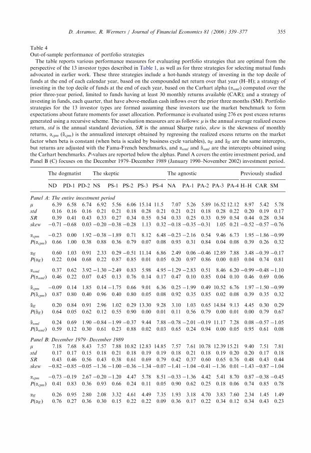
Here, we analyze the ex post, out-of-sample performance of various portfolios strategiesthrough a sequence of investments with monthly rebalancing. Optimal portfolios arederived first using the initial 60 monthly observations, then using the first 61 monthlyobservations, and so on, . . . ; and are finally rebalanced using the first T � 1 monthlyobservations, with T ¼ 336 denoting the sample size. Hence, the first investment is made atthe end of December 1979, the second at the end of January 1980, and so on, . . . ; with thelast at the end of November 2002. We obtain the month-t realized excess return on eachinvestment strategy by multiplying the portfolio weights of month t� 1 by the month-trealized excess returns of the corresponding mutual funds. This recursive scheme produces276 excess returns on 13 investment strategies that differ with respect to the Bayesianpredictive moments used in the portfolio optimization.Table 4 reports various performance measures, described below, for evaluating portfolio

strategies that are optimal from the perspective of the 13 investor types as well as for threeother strategies for selecting mutual funds that have been proposed in past work. Thesethree strategies include a ‘‘hot-hands’’ strategy of investing in the top decile of funds at theend of each calendar year, based on the compounded net return over that year (H–H), astrategy of investing in the top decile of funds at the end of each year, based on theCarhart alpha (awml) computed over the prior three-year period, limited to funds that haveat least 30 monthly returns available (CAR), and a strategy of investing in funds, eachquarter, that have above-median cash inflows (among all positive cash-inflow funds)during the prior three months (SM). The first 13 portfolio strategies are formed assumingthat investors use only the market benchmark (MKT) to form moments for assetallocation.In Table 4, m is the average realized excess return, SR is the annual Sharpe ratio, skew is

the skewness of monthly returns, acpm (~acpm) is the intercept obtained by regressing therealized excess returns on the market factor when beta is constant (when beta is scaled bybusiness cycle variables), aff and ~aff are the same intercepts, but returns are adjusted withthe Fama-French benchmarks (MKT, SMB, and HML), and awml and ~awml are theintercepts obtained using the Carhart benchmarks (MKT, SMB, HML, and WML);p-values are reported below the alphas. All alpha measures as well as m are shown in % perannum. Panel A covers the entire investment period, while Panel B (C) focuses on theDecember 1979–December 1989 (January 1990–November 2002) investment period. Thefirst subperiod corresponds to the time before the discovery of the macro variables byKeim and Stambaugh (1986) and Fama and French (1989). The second subperiod capturesthe post-discovery period.Although we form optimal portfolios for believers in the CAPM, out-of-sample ex post

performance is assessed using the CAPM, the Fama-French three-factor model, and theCarhart four-factor model. That is, we assume that the performance evaluator observes theinvestment returns, but does not know the model that generates the returns, and therefore,implements various performance measures. Note that a positive and significant acpm (~acpm)implies that the evaluated investment outperforms a static (dynamic) investment in themarket benchmark, generating higher payoffs for the same fixed (time-varying) riskexposures. Performance measures under the Fama-French and Carhart models should besimilarly interpreted; that is, they imply that the evaluated investment outperforms a staticor dynamic investment with the same exposures to the multiple risk sources.

ARTICLE IN PRESS

Table 4

Out-of-sample performance of portfolio strategies

The table reports various performance measures for evaluating portfolio strategies that are optimal from the

perspective of the 13 investor types described in Table 1, as well as for three strategies for selecting mutual funds

advocated in earlier work. These three strategies include a hot-hands strategy of investing in the top decile of

funds at the end of each calendar year, based on the compounded net return over that year (H–H); a strategy of

investing in the top decile of funds at the end of each year, based on the Carhart alpha (awml ) computed over the

prior three-year period, limited to funds having at least 30 monthly returns available (CAR); and a strategy of

investing in funds, each quarter, that have above-median cash inflows over the prior three months (SM). Portfolio

strategies for the 13 investor types are formed assuming these investors use the market benchmark to form

expectations about future moments for asset allocation. Performance is evaluated using 276 ex post excess returns

generated using a recursive scheme. The evaluation measures are as follows: m is the annual average realized excess

return, std is the annual standard deviation, SR is the annual Sharpe ratio, skew is the skewness of monthly

returns, acpm ð~acpmÞ is the annualized intercept obtained by regressing the realized excess returns on the market

factor when beta is constant (when beta is scaled by business cycle variables), aff and ~aff are the same intercepts,

but returns are adjusted with the Fama-French benchmarks, and awml and ~awml are the intercepts obtained using

the Carhart benchmarks. P-values are reported below the alphas. Panel A covers the entire investment period, and

Panel B (C) focuses on the December 1979–December 1989 (January 1990–November 2002) investment period.

The dogmatist The skeptic The agnostic Previously studied

ND PD-1 PD-2 NS PS-1 PS-2 PS-3 PS-4 NA PA-1 PA-2 PA-3 PA-4 H–H CAR SM

Panel A: The entire investment period

m 6.39 6.58 6.74 6.92 5.56 6.06 15.14 11.5 7.07 5.26 5.89 16.52 12.12 8.97 5.42 5.78

std 0.16 0.16 0.16 0.21 0.21 0.18 0.28 0.21 0.21 0.21 0.18 0.28 0.22 0.20 0.19 0.17

SR 0.39 0.41 0.43 0.33 0.27 0.34 0.55 0.54 0.33 0.25 0.33 0.59 0.54 0.44 0.28 0.34

skew �0.71 �0.68 0.03 �0.20 �0.38 �0.28 1.13 0.32 �0.18 �0.35 �0.31 1.05 0.21 �0.52 �0.57 �0.76

acpm �0.23 0.00 1.92 �0.38 �1.89 0.71 8.12 6.48 �0.23 �2.16 0.54 9.46 6.73 1.95 �1.86 �0.99

PðacpmÞ 0.66 1.00 0.38 0.88 0.36 0.79 0.07 0.08 0.93 0.31 0.84 0.04 0.08 0.39 0.26 0.32

aff 0.60 1.03 0.91 2.33 0.29 �0.51 11.14 6.86 2.49 0.06 �0.46 12.89 7.88 3.48 �0.39 �0.17

Pðaff Þ 0.22 0.04 0.68 0.22 0.87 0.85 0.01 0.05 0.20 0.97 0.86 0.00 0.03 0.04 0.74 0.81

awml 0.37 0.62 3.92 �1.30 �2.49 0.83 5.98 4.95 �1.29 �2.83 0.51 8.46 6.20 �0.99 �0.48 �1.10

Pðawml Þ 0.46 0.22 0.07 0.45 0.13 0.76 0.14 0.17 0.47 0.10 0.85 0.04 0.10 0.46 0.69 0.06

~acpm �0.09 0.14 1.85 0.14 �1.75 0.66 9.01 6.36 0.25 �1.99 0.49 10.52 6.76 1.97 �1.50 �0.99

Pð~acpmÞ 0.87 0.80 0.40 0.96 0.40 0.80 0.05 0.08 0.92 0.35 0.85 0.02 0.08 0.39 0.35 0.32

~aff 0.20 0.84 0.91 2.96 1.02 0.29 13.30 9.28 3.10 1.03 0.65 14.84 9.13 4.45 0.30 0.29

Pð~aff Þ 0.64 0.05 0.62 0.12 0.55 0.90 0.00 0.01 0.11 0.56 0.79 0.00 0.01 0.00 0.79 0.67

~awml 0.24 0.69 1.90 �0.84 �1.99 �0.37 9.44 7.88 �0.78 �2.01 �0.19 11.17 7.28 0.08 �0.57 �1.05

Pð~awml Þ 0.59 0.12 0.30 0.61 0.23 0.88 0.02 0.03 0.65 0.24 0.94 0.00 0.05 0.95 0.61 0.08

Panel B: December 1979– December 1989

m 7.18 7.68 8.43 7.57 7.88 10.82 12.83 14.85 7.57 7.61 10.78 12.39 15.21 9.40 7.51 7.81

std 0.17 0.17 0.15 0.18 0.21 0.18 0.19 0.19 0.18 0.21 0.18 0.19 0.20 0.20 0.17 0.18

SR 0.43 0.46 0.56 0.43 0.38 0.61 0.69 0.79 0.42 0.37 0.60 0.65 0.76 0.48 0.43 0.44

skew �0.82 �0.85 �0.05 �1.36 �1.00 �0.36 �1.34 �0.07 �1.41 �1.04 �0.41 �1.36 0.01 �1.43 �0.87 �1.04

acpm �0.73 �0.19 2.67 �0.20 �1.20 4.47 5.78 8.51 �0.33 �1.36 4.42 5.41 8.70 0.87 �0.38 �0.45

PðacpmÞ 0.41 0.83 0.36 0.93 0.66 0.24 0.11 0.05 0.90 0.62 0.25 0.18 0.06 0.74 0.85 0.78

aff 0.26 0.95 2.80 2.08 3.32 4.61 4.49 7.35 1.93 3.18 4.70 3.83 7.60 2.34 1.45 1.49

Pðaff Þ 0.76 0.27 0.36 0.30 0.15 0.22 0.22 0.09 0.36 0.17 0.22 0.34 0.12 0.34 0.43 0.23

D. Avramov, R. Wermers / Journal of Financial Economics 81 (2006) 339–377 355

ARTICLE IN PRESS

Table 4 (continued )

The dogmatist The skeptic The agnostic Previously studied

ND PD-1 PD-2 NS PS-1 PS-2 PS-3 PS-4 NA PA-1 PA-2 PA-3 PA-4 H–H CAR SM

awml 0.20 0.79 3.40 �0.58 0.39 4.12 0.52 5.39 �0.85 0.24 4.17 �0.16 5.17 �1.42 �0.10 �0.36

PðawmlÞ 0.82 0.36 0.27 0.74 0.85 0.29 0.88 0.22 0.64 0.91 0.29 0.97 0.29 0.48 0.95 0.73

~acpm �0.70 �0.18 1.63 �0.67 �1.48 3.33 5.56 7.08 �0.80 �1.67 3.19 5.16 7.21 0.73 �0.89 �0.74

Pð~acpmÞ 0.43 0.84 0.56 0.78 0.59 0.36 0.13 0.08 0.75 0.55 0.39 0.20 0.11 0.78 0.66 0.64

~aff �0.27 0.46 �2.30 3.54 5.25 2.39 5.26 5.47 3.35 5.33 2.63 4.98 5.24 6.28 2.14 1.79

Pð~aff Þ 0.76 0.59 0.38 0.05 0.03 0.50 0.12 0.18 0.08 0.03 0.47 0.20 0.25 0.01 0.28 0.17

~awml 0.01 0.76 �1.95 0.95 1.40 1.63 0.88 2.20 0.75 1.46 1.67 0.27 1.04 1.52 �1.23 �1.04

Pð~awmlÞ 0.99 0.39 0.46 0.55 0.54 0.63 0.79 0.61 0.65 0.52 0.63 0.94 0.83 0.48 0.51 0.32

Panel C: January 1990– November 2002

m 5.78 5.73 5.44 6.55 3.79 2.39 16.45 8.93 6.88 3.44 2.13 19.69 9.83 8.8 4.6 4.69

std 0.16 0.16 0.16 0.23 0.21 0.18 0.32 0.23 0.24 0.22 0.18 0.33 0.25 0.20 0.20 0.16

SR 0.36 0.36 0.34 0.28 0.18 0.13 0.51 0.39 0.29 0.16 0.12 0.59 0.40 0.43 0.23 0.29

skew �0.61 �0.55 0.08 0.18 0.10 �0.21 1.35 0.51 0.23 0.15 �0.24 1.26 0.31 0.04 �0.44 �0.53

acpm 0.19 0.17 1.37 �0.31 �2.40 �2.14 10.10 4.90 0.03 �2.74 �2.39 12.83 5.25 2.23 �2.82 �1.62

PðacpmÞ 0.75 0.81 0.66 0.93 0.43 0.55 0.18 0.38 0.99 0.38 0.50 0.09 0.37 0.50 0.20 0.17

aff 0.91 1.09 0.15 2.04 �1.29 �3.63 13.68 5.47 2.42 �1.61 �3.67 16.99 6.72 3.90 �1.55 �1.04

Pðaff Þ 0.09 0.06 0.96 0.48 0.60 0.31 0.03 0.28 0.41 0.53 0.30 0.01 0.20 0.08 0.23 0.14

awml 0.51 0.45 4.91 �3.26 �4.20 �1.25 6.79 3.65 �3.01 �4.76 �1.90 11.15 5.40 �1.79 �1.25 �2.35

PðawmlÞ 0.34 0.44 0.08 0.19 0.08 0.73 0.27 0.49 0.23 0.05 0.60 0.07 0.32 0.28 0.36 0.00

~acpm 0.36 0.37 1.82 0.10 �1.64 �1.48 11.90 6.14 0.43 �1.91 �1.68 14.58 6.61 2.28 �2.46 �1.40

Pð~acpmÞ 0.54 0.59 0.56 0.98 0.58 0.68 0.11 0.27 0.91 0.54 0.63 0.05 0.25 0.49 0.27 0.24

~aff 0.67 1.19 1.95 1.42 �1.18 �2.62 17.39 10.28 1.97 �1.32 �2.43 19.77 9.96 3.09 �1.28 �1.04

Pð~aff Þ 0.07 0.01 0.37 0.59 0.59 0.39 0.00 0.03 0.47 0.56 0.43 0.00 0.05 0.08 0.30 0.09

~awml 0.74 0.81 2.14 �3.49 �3.79 �3.66 14.23 8.76 �2.99 �3.66 �3.63 15.83 6.80 �1.21 �1.28 �2.05

Pð~awmlÞ 0.06 0.07 0.34 0.15 0.08 0.24 0.02 0.09 0.23 0.10 0.25 0.01 0.20 0.41 0.32 0.00

D. Avramov, R. Wermers / Journal of Financial Economics 81 (2006) 339–377356

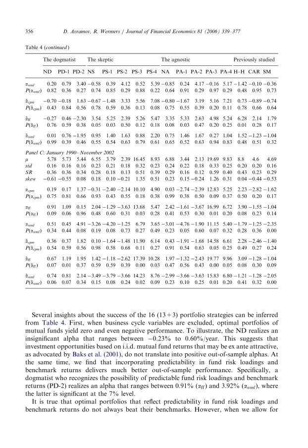
Several insights about the success of the 16 (13+3) portfolio strategies can be inferredfrom Table 4. First, when business cycle variables are excluded, optimal portfolios ofmutual funds yield zero and even negative performance. To illustrate, the ND realizes aninsignificant alpha that ranges between �0.23% to 0.60%/year. This suggests thatinvestment opportunities based on i.i.d. mutual fund returns that may be ex ante attractive,as advocated by Baks et al. (2001), do not translate into positive out-of-sample alphas. Atthe same time, we find that incorporating predictability in fund risk loadings andbenchmark returns delivers much better out-of-sample performance. Specifically, adogmatist who recognizes the possibility of predictable fund risk loadings and benchmarkreturns (PD-2) realizes an alpha that ranges between 0.91% (aff ) and 3.92% ðawml), wherethe latter is significant at the 7% level.It is true that optimal portfolios that reflect predictability in fund risk loadings and

benchmark returns do not always beat their benchmarks. However, when we allow for

ARTICLE IN PRESSD. Avramov, R. Wermers / Journal of Financial Economics 81 (2006) 339–377 357

predictability in manager skills, we find that the resulting optimal portfolios consistentlyoutperform strategies that exclude predictability, strategies that account for predictablefund risk loadings and benchmark returns only, static and dynamic investments in theFama-French and momentum benchmarks, and the three previously studied strategies thatwe describe above.

To illustrate the strong performance of strategies that account for predictable managerskills, we note that the PA-3 investor selects optimal portfolios that generate acpm ¼ 9:46%,~acpm ¼ 10:52%, aff ¼ 12:89%, ~aff ¼ 14:84%, awml ¼ 8:46%, and ~awml ¼ 11:17%, all ofwhich are significant at the 5% level. Moreover, the out-of-sample Sharpe ratios ofstrategies that reflect predictability in manager skills are the largest, consistent with the exante results described earlier. Take, for instance, the agnostic investor. When predictabilityis disregarded altogether (NA), the annual Sharpe ratio is 0.33. Allowing for predictabilityin fund risk loadings and benchmark assets (PA-2) does not change this Sharpe ratio.However, allowing for predictability in manager skills (PA-3) delivers a much larger Sharperatio of 0.59.

Note, also, that the skewness of investment returns is much larger for strategies thatinclude predictable manager skills. For instance, the level of skewness is 1.05 for investorPA-3, whereas skewness is negative for all investors who disregard predictability, such asinvestor NA. Although we consider only investor types who are mean-variance optimizers,the higher skewness obtained by PA-3 and other predictable skills strategies indicate thatinvestors who directly include skewness in their preferences (such as those that have apower utility function) would prefer these optimal portfolios relative to those obtained byNA and other no-predictability strategies. That is, the higher levels of skewness indicatethat predictable skills strategies may be attractive to an even broader set of investor typesthan those considered in this paper.

Interestingly, none of the previously studied strategies, H–H, CAR, and SM, produceperformance that matches the optimal portfolios that use predictability in skills. The CARand SM generate mostly negative alphas. The H–H strategy generates a positive andsignificant aff and ~aff of 3.48% and 4.45%, respectively. However, this performancebecomes insignificant when adding a momentum factor, consistent with Carhart (1997),suggesting that our portfolio strategies are unique, and that they outperform optimalstrategies that exclude conditioning information as well as strategies that pick funds basedon past returns and flows, as advocated previously in the mutual fund literature.

We conduct two additional experiments. First, we implement the same performancemeasures for two subperiods, namely, the investment period December 1979–December1989 (Panel B, Table 4), and the investment period January 1990–November 2002 (PanelC). Second, we analyze performance (see Table 5) when optimal portfolios are formed bythe 13 types of investors that believe in the Fama-French model as well as the Carhartfour-factor model.

Studying two subperiods is important because the mutual fund industry has grown overtime with many more funds available for investment in the second part of the sample.Moreover, through this subperiod analysis, we attempt to address data-mining concerns.Specifically, Schwert (2003) notes that the so-called financial market anomalies related toprofit opportunities tend to disappear, reverse, or attenuate following their discovery. Forexample, he shows that the relation between the aggregate dividend yield and the equitypremium is much weaker after the discovery of that predictor by Keim and Stambaugh(1986) and Fama and French (1989).

ARTICLE IN PRESS

Table 5

Out-of-sample performance of optimal portfolio strategies

The table reports various performance measures for evaluating portfolio strategies that are optimal from the

perspective of the 13 investor types described in Table 1, using the Fama-French model and the Carhart (1997)

models to form moments for asset allocation. Performance is evaluated using 276 ex post excess returns generated

using a recursive scheme. The evaluation measures are as follows: m is the average realized excess return, acpm

(~acpm) is the intercept obtained by regressing the realized excess returns on the market factor when beta is constant

(when beta is scaled by business cycle variables), aff and ~aff are the same intercepts, but returns are adjusted with

the Fama-French benchmarks, and awml and ~awml are the intercepts obtained using the Carhart benchmarks. All

measures are percent per annum. The symbols � and �� reflect significance at the 5% and 10% levels, respectively.

The dogmatist The skeptic The agnostic

ND PD-1 PD-2 NS PS-1 PS-2 PS-3 PS-4 NA PA-1 PA-2 PA-3 PA-4

The Fama-French model

m 6.64 6.24 5.86 6.57 4.56 6.25 11.11 10.24 6.65 4.68 6.24 11.17 10.26

acpm 1.68 1.05 1.00 �0.01 �2.37 0.36 4.57 4.96 �0.10 �2.35 0.30 4.51 4.53

aff �2.00 �1.60 �0.71 1.09 �0.99 0.77 8.35* 5.00 1.37 �0.68 0.95 9.09* 5.13

awml �1.36 �2.47 �1.56 �1.50 �3.07 �0.11 2.98 3.00 �1.32 �2.65 0.12 4.11 3.10

~acpm 1.21 0.61 0.42 0.36 �2.00 0.62 5.67 4.96 0.30 �1.93 0.57 5.70 4.60

~aff �1.33 �0.51 0.82 2.34 1.22 2.92 12.38* 7.67* 2.77 1.65 3.04 12.80* 7.41*

~awml �0.46 �1.30 �1.03 �0.32 �1.71 0.74 8.89* 5.99 0.04 �1.21 0.87 9.35* 5.13

The Carhart model

m 3.43 8.67 5.11 5.82 8.42 5.17 10.80 10.38 5.95 8.35 5.40 11.73 10.62

acpm �1.48 3.25 �0.07 �0.75 2.24 �0.92 4.12 4.78 �0.75 2.08 �0.74 5.02 4.45

aff �3.41 2.95 �0.50 0.16 4.10** 0.25 7.33** 5.17** 0.47 4.17** 0.56 9.15* 5.80**

awml �5.13* 0.27 �3.87 �2.12 2.42 �2.03 2.30 2.49 �1.92 2.68 �1.59 4.16 3.14

~acpm �1.82 3.07 �0.27 �0.39 2.73 �0.61 5.12 4.83 �0.32 2.64 �0.42 6.18 4.67

~aff �2.26 3.98** 1.31 1.69 4.54** 2.17 10.96* 6.97* 2.24 4.63* 2.39 12.96* 6.77*

~awml �3.48 1.60 �2.01 �0.63 2.56 �0.55 7.71* 4.77 �0.19 2.75 �0.21 9.47* 4.56

D. Avramov, R. Wermers / Journal of Financial Economics 81 (2006) 339–377358

Observe from Table 4, Panel C that, over the second subperiod, the PA-3 strategyproduces robust performance measures. Specifically, the Sharpe ratio attributable to thatstrategy, 0.59, continues to be the largest across all strategies. In addition, all (annual)alphas are large and significant, given by acpm ¼ 12:83%, ~acpm ¼ 14:58%, aff ¼ 16:99%,~aff ¼ 19:77%, awml ¼ 11:15%, and ~awml ¼ 15:83%. Indeed, much of the remarkableperformance of the PA-3 strategy can be traced to this second subperiod, during whichtime the predictive variables are already known and available for investment, and when theinvestment universe contains many more funds.Finally, observe from Table 5 that the superior performance of strategies that allow for

predictability in manager skills also obtains when the three Fama-French benchmarks andthe four Carhart benchmarks are used to form optimal portfolios. Such strategiesconsistently deliver positive alphas that are often significant at the 5% or 10% level. Alsonote that optimal trading strategies that exclude predictability altogether mostly generateinsignificant levels of performance. Overall, the finding that predictability in manager skillsis the dominant source of investment profitability still prevails under these alternativemodels.We note that the findings in Moskowitz (2000) suggest that fund performance may

vary with the business cycle. Moskowitz (2000) uses the NBER characterization for

ARTICLE IN PRESSD. Avramov, R. Wermers / Journal of Financial Economics 81 (2006) 339–377 359

recessionary and expansionary periods, and documents higher performance duringrecessions, relative to expansions, using the difference in portfolio holdings basedperformance measures or the difference in net returns. Our work shows that fundperformance varies predictably (and substantially) with predetermined macroeconomicvariables. Moreover, explicitly incorporating predictability in manager skills using suchmacro variables leads to dramatically different optimal portfolios of equity mutual funds.In our framework, one can identify ex ante the best performing funds, leading to anoptimal fund-of-funds that outperforms dynamic and static investments in passivebenchmarks as well as other strategies previously studied in the mutual fund context.Overall, our findings suggest that active mutual fund management adds much more valuethan previously recognized.

4.3. The determinants of the superior predictability-based performance

What explains the remarkable performance of strategies that account for predictableskills? In this section, we attempt to address this question. We study the attributes ofthese strategies at the stock holdings and net returns levels, and we explore inter- andintraindustry effects in their portfolio allocations.

4.3.1. Attributes of portfolio strategies

We first examine the attributes of our optimally selected portfolios of equity mutualfunds. Table 6 provides time-series average portfolio-level and fund-level attributes acrossall 276 investment periods (December 1979–November 2002), as well as averages acrossNBER expansions only, and across NBER recessions only.

Portfolio holdings attributes of mutual funds include the time-series averagecharacteristic selectivity performance measure of Daniel, Grinblatt, Titman, and Wermers(DGTW; 1997) in percent per year (CS), as well as its p-value, and the size (Size), book-to-market (BTM), and momentum (MOM) nonparametric rank characteristics of thestockholdings, as defined by DGTW. To compute the CS measure as well asnonparametric characteristics of the stockholdings of each fund, we follow DGTW increating portfolios, for each stock during each year, that closely match the size, book-to-market, and momentum characteristics of that stock.6 In turn, these portfolio holdingsattributes of funds are weighted by each investor’s optimal fund holdings to arrive atinvestor-level attributes. To illustrate, the ND investor records a CS measure of 0.39%/year over the entire investment period, 0.23% over expansions, and 1.25% over recessions.

These portfolio-level and fund-level attributes provide insights into the types of mutualfunds that the different optimal strategies choose to hold. Let us start with the CS measure.There are two notable findings here. First, the CS measure indicates that funds selected by

6To be specific, we sort all CRSP stocks, conditionally, into quintiles based on their size, book-to-market, and

momentum characteristics on June 30 of each year, thereby forming 125 portfolios (e.g., the portfolio identified as

5,5,5 is the large-capitalization, high book-to-market, high momentum stock portfolio). Then, the characteristic-

adjusted return for each stock, from July 1 to June 30 of the following year, is the return on the stock minus the

return on the value-weighted portfolio to which that stock belongs. The CS measure for a given fund is computed

as the portfolio-weighted characteristic-adjusted return during each month of that fund’s existence. The

nonparametric size characteristic for a given fund is the quintile size portfolio number to which each stock belongs

during a given year, weighted across all stocks held by the fund each month. The BTM and MOM nonparametric

characteristics of each fund are computed similarly.

ARTICLE IN PRESS

Table

6

Attributesofoptimalportfolios

Thetablereportsseveralattributesoftheportfoliostrategiesthatare

optimalfrom

theperspectiveofthe13investortypes

described

inTable1,aswellasforthree

strategiesforselectingmutualfundsthatappearin

previousstudies,asexplained

inTable4.Theseattributesincludetheportfolio-w

eightedcharacteristicselectivity

measure

inpercentper

year(C

S),aswellasits

p-value(inparentheses),lagged

net

return,compounded

over

the12monthspriorto

each

portfolioform

ationdate

(Lag12ðR

etÞ),totalnet

assetsin

millionsofdollars(T

NA)offunds,portfolioholdings-basedDGTW

(nonparametric)

styleattributesin

thesize

(Siz

e),book-to-m

arket

(BT

M),andmomentum

(MO

M)dim

ensions,percentmonthly

fundturnover,computedasannualreported

turnover

divided

by12(T

urn

ove

r),monthly

percentage

net

cash

inflows(F

low),computedas

TN

Aminusone-quarter-lagged

TN

A(adjusted

forinvestm

entreturnsanddistributions),divided

bythree,

fundexpense

ratio

(Ex

pen

seR

ati

o),portfolioweightallocationto

index

funds(I

nd

exF

un

ds),andleadmanager

experience

inmonths(M

an

ager

Ex

per

ien

ce).Theseattributesare

presented

forallperiods,forexpansionsonly,andforrecessionsonly.

Thedogmatist

Theskeptic

Theagnostic

Previouslystudied

ND

PD-1

PD-2

NS

PS-1

PS-2

PS-3

PS-4

NA

PA-1

PA-2

PA-3

PA-4

H–H

CAR

SM

Ove

rall

CS

0.39

0.26

2.13

0.57

1.47

2.99

7.19

4.38

0.47

1.06

2.78

8.10

6.02

3.30

0.38

1.84

PðC

SÞ

0.28

0.51

0.36

0.72

0.36

0.38

0.09

0.31

0.77

0.51

0.42

0.05

0.19

0.08

0.82

0.05

Lag12ðR

etÞ

7.92

8.75

8.54

26.89

22.68

17.53

37.71

28.70

26.69

22.55

17.68

38.73

29.58

29.78

19.33

19.56

TN

A388.73

343.74

201.40

343.47

296.58

224.68

170.39

149.13

318.45

286.68

216.20

146.77

139.68

175.61

195.34

243.97

Siz

e4.58

4.62

4.05

3.61

4.04

3.69

3.62

3.61

3.52

3.99

3.63

3.55

3.60

3.63

3.68

3.95

BT

M2.70

2.72

2.70

2.51

2.49

2.44

2.45

2.47

2.53

2.49

2.43

2.48

2.44

2.52

2.51

2.62

MO

M3.01

3.03

2.98

3.81

3.88

3.44

3.66

3.35

3.79

3.86

3.45

3.61

3.39

3.70

3.41

3.40

Turn

ove

r1.71

1.91

3.79

9.01

9.29

7.72

8.37

7.85

9.29

9.53

8.05

8.75

7.49

8.43

8.44

7.56

Flo

w2.57

2.49

3.51

5.23

4.52

4.67

6.75

6.54

5.47

4.69

4.93

7.28

6.96

5.91

4.54

6.01

Ex

pen

seR

ati

o0.02

0.02

0.08

0.11

0.11

0.11

0.11

0.11

0.11

0.11

0.11

0.12

0.11

0.11

0.11

0.09

Ind

exF

un

ds

0.54

0.52

0.15

0.03

0.02

0.02

0.02

0.01

0.03

0.03

0.02

0.02

0.01

0.02

0.01

0.08

Ma

na

ger

Ex

per

ien

ce85.53

88.61

123.46

155.84

179.45

120.79

120.24

111.92

148.33

171.58

117.97

108.92

106.46

99.11

105.77

97.92

Ex

pa

nsi

on

s

CS

0.23

0.10

1.29�0.93�0.11

0.63

5.45

2.68�0.91�0.01

0.41

7.19

5.14

2.89

0.37

1.37

PðC

SÞ

0.58

0.82

0.61

0.60

0.95

0.87

0.23

0.56

0.62

0.99

0.92

0.12

0.30

0.16

0.82

0.16

Lag12ðR

etÞ

8.94

9.83

10.60

28.86

25.37

20.15

41.76

32.75

28.69

25.23

20.24

42.68

33.73

31.84

21.85

21.88

D. Avramov, R. Wermers / Journal of Financial Economics 81 (2006) 339–377360

ARTICLE IN PRESST

NA

403.78

354.54

194.70

375.00

316.34

233.05

180.75

159.07

347.75

304.64

223.50

154.80

144.70

182.07

201.74

250.87

Siz

e4.59

4.63

4.08

3.70

4.09

3.73

3.68

3.68

3.60

4.03

3.66

3.59

3.66

3.63

3.67

3.97

BT

M2.70

2.73

2.81

2.50

2.55

2.50

2.42

2.51

2.52

2.56

2.49

2.44

2.49

2.52

2.52

2.65

MO

M3.04

3.05

2.95

3.80

3.84

3.41

3.68

3.35

3.78

3.83

3.40

3.62

3.38

3.71

3.44

3.40

Turn

ove

r1.71

1.91

3.79

9.01

9.29

7.72

8.37

7.85

9.29

9.53

8.05

8.75

7.49

8.43

8.44

7.56

Flo

w2.63

2.54

3.60

4.89

4.48

4.59

6.75

6.56

5.16

4.63

4.88

7.20

7.09

5.96

4.58

6.09

Ex

pen

seR

ati

o0.02

0.02

0.08

0.11

0.11

0.11

0.11

0.11

0.11

0.11

0.11

0.12

0.11

0.11

0.11

0.09

Ind

exF

un

ds

0.56

0.54

0.13

0.04

0.03

0.02

0.02

0.01

0.04

0.03

0.03

0.02

0.01

0.02

0.01

0.09

Ma

na

ger

Ex

per

ien

ce89.67

91.70

120.10

160.45

176.23

117.91

120.57

111.17

152.26

167.70

114.93

105.88

105.11

96.60

102.17

95.34

Rec

essi

on

s

CS

1.25

1.07

9.47

9.12

10.25

14.62

11.28

11.99

8.24

7.19

14.38

13.86

8.81

6.63

0.42

4.38

PðC

SÞ

0.13

0.18

0.07

0.00

0.07

0.06

0.20

0.31

0.00

0.18

0.05

0.09

0.43

0.00

0.80

0.13

Lag12ðR

etÞ

1.53

2.00�4.36

14.56

5.84

1.10

12.32

3.28

14.19

5.72

1.65

14.00

3.55

16.92

3.54

5.05

TN

A294.91

276.12

242.66

159.24

176.95

176.90

106.01

87.68

155.00

177.99

174.76

91.68

108.41

135.09

155.26

200.77

Siz

e4.55

4.53

3.82

3.06

3.73

3.49

3.26

3.22

2.98

3.72

3.47

3.31

3.24

3.61

3.75

3.82

BT

M2.74

2.72

2.10

2.62

2.13

2.10

2.65

2.17

2.60

2.09

2.08

2.68

2.16

2.52

2.45

2.48

MO

M2.85

2.89

3.17

3.85

4.08

3.67

3.48

3.39

3.83

4.06

3.69

3.54

3.47

3.64

3.28

3.36

Turn

ove

r2.45

2.39

3.96

7.55

9.37

7.87

9.71

11.00

7.86

9.51

7.95

9.88

9.80

7.97

10.73

7.03

Flo

w2.09

2.09

3.00

7.21

4.75

5.08

6.76

6.40

7.21

5.00

5.21

7.89

6.25

5.61

4.35

5.50

Ex

pen

seR

ati

o0.03

0.03

0.08

0.10

0.10

0.10

0.11

0.11

0.11

0.11

0.11

0.11

0.10

0.11

0.11

0.09

Ind

exF

un

ds

0.41

0.40

0.24

0.00

0.00

0.00

0.00

0.01

0.00

0.00

0.00

0.00

0.00

0.01

0.02

0.07

Ma

na

ger

Ex

per

ien

ce59.78

68.67

147.42

127.21

199.60

139.71

118.21

116.54

124.74

195.85

137.60

129.70

115.17

114.85

128.32

114.06

D. Avramov, R. Wermers / Journal of Financial Economics 81 (2006) 339–377 361

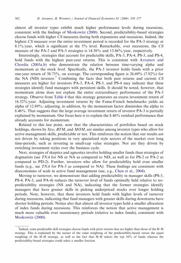
ARTICLE IN PRESSD. Avramov, R. Wermers / Journal of Financial Economics 81 (2006) 339–377362

almost all investor types exhibit much higher performance levels during recessions,consistent with the findings of Moskowitz (2000). Second, predictability-based strategieschoose funds with higher CS measures during both expansions and recessions. Indeed, thehighest CS measure over the entire investment period is recorded for the PA-3 strategy at8.1%/year, which is significant at the 5% level. Remarkably, over recessions, the CS

measure of the PA-2 and PA-3 strategies is 14.38% and 13.86%/year, respectively.Interestingly, strategies that account for predictable skills, PA-3, PA-4, PS-3, and PS-4,

hold funds with the highest past-year returns. This is consistent with Avramov andChordia (2005a,b) who demonstrate the relation between time-varying alpha andmomentum at the stock level. Specifically, the PA-3 investor holds funds with a priorone-year return of 38.73%, on average. The corresponding figure is 26.69% (7.92%) forthe NA (ND) investor.7 Combining the facts that both past returns and current CS

measures are higher for investors PA-3, PA-4, PS-3, and PS-4 may indicate that thesestrategies identify fund managers with persistent skills. It should be noted, however, thatmomentum alone does not explain the entire extraordinary performance of the PA-3strategy. Observe from Table 4 that this strategy generates an excess investment return of16.52%/year. Adjusting investment returns by the Fama-French benchmarks yields analpha of 12.89%; adjusting, in addition, by the momentum factor diminishes the alpha to8.46%. That suggests that the large average investment return of investor PA-3 is partiallyexplained by momentum. Our focus here is to explain the 8.46% residual performance thatalready accounts for momentum.Related to this last point, note that the characteristics of portfolios based on stock

holdings, shown by Size, BTM, and MOM, are similar among investor types who allow foractive management skills, predictable or not. This reinforces the notion that our results arenot driven by taking positions in very specialized style sectors of the market over longtime-periods, such as investing in small-cap value strategies. Nor are they driven byswitching investment styles over the business cycle.Next, strategies of skeptics and agnostics involve holding smaller funds than strategies of

dogmatists (see TNA for NS or NA as compared to ND, as well as for PS-2 or PA-2 ascompared to PD-2). Further, investors who allow for predictability hold even smallerfunds (e.g., see TNA for PA-3 as compared to NA). These findings are consistent withdiseconomies of scale in active fund management (see, e.g., Chen et al., 2004).Moving to turnover, we demonstrate that adding predictability in manager skills (PS-3,

PS-4, PA-3, and PA-4) reduces the turnover level of funds optimally held relative to no-predictability strategies (NS and NA), indicating that the former strategies identifymanagers that have greater skills in picking underpriced stocks over longer holdingperiods. Note, however, that these investors hold funds with higher levels of turnoverduring recessions, indicating that fund managers with greater skills during downturns haveshorter holding periods. Notice also that almost all investor types hold a smaller allocationof index funds during recessions. This reinforces the notion that active management ismuch more valuable over recessionary periods (relative to index funds), consistent withMoskowitz (2000).

7Indeed, some predictable skill strategies choose funds with prior returns that are higher than those of the H–H

strategy. This is explained by the nature of the value weighting of the predictability-based versus the equal

weighting of the H–H strategy, as well as the fact that H–H selects the top 10% of funds whereas the

predictability-based strategies could select a smaller fraction.

ARTICLE IN PRESSD. Avramov, R. Wermers / Journal of Financial Economics 81 (2006) 339–377 363

The pattern of flows indicates that investors who believe in active management skillsfollow funds with higher levels of lagged net inflows, which is not surprising since theyhave higher allocations to funds that have high past returns, and flows and past returnshave been shown to be highly correlated (see, e.g., Sirri and Tufano, 1998). However,strategies PS-3, PS-4, PA-3, and PA-4 do not merely capture the smart money effectbecause, as Table 4 highlights, a strategy that merely selects funds based on their flowsproduces negative performance relative to the Fama-French and momentum benchmarks.

The level of manager experience indicates that predictability-based strategies involvechoosing fund managers with slightly less experience, but this trend does not seemespecially strong.

For comparison purposes, we also present portfolio attributes for the hot-hands,Carhart, and smart money strategies discussed previously. We find that these strategiesgenerally involve holding funds with similar fund-level and portfolio-level attributes asinvestors PA-3 and PA-4, but that they do not generate similar levels of CS performance.Thus, predictability-based strategies involve selecting from similar groups of funds as themore mechanical hot-hands, Carhart, and smart money strategies, but are much moresuccessful in identifying manager talents.

We summarize the evidence emerging from this section as follows. Strategies thataccount for predictable manager skills outperform their characteristic-based benchmarks,especially during recessions. Such strategies pick funds with higher past one-yearreturns and funds with higher new money inflows. Even so, their overall extraordinaryperformance is unexplained by following mechanical trading strategies based on flows ormomentum because the hot-hand and smart money strategies that exploit information inpast returns and new money inflows do not produce such robust performance measures. Inaddition, the outperforming predictability-based strategies hold stocks with similar size,book-to-market, and momentum characteristics as those held by other less promisingstrategies. However, although the average TNA is different across the strategies, this doesnot explain the dispersion in performance. Specifically, Chen et al. (2004) find a differencein performance of only 1%/year between the smallest and largest quintiles of mutual funds.Thus, we need to look for other sources, beyond the characteristic styles, past fund returns,and new money inflows, or fund TNA, to explain the disparity in performance among thecompeting strategies. We turn to this issue next.

4.3.2. Industry allocation analysis

Specifically, we examine whether inter- and intraindustry effects can explain thedispersion in performance among trading strategies. In particular, we consider 13industries based on the Fama-French 12-industry classification, plus a separate industrycategory for stocks in the metals mining and metals wholesaling businesses.8 The 13industries include: computer hardware, software, and other electronic equipment (Buseq);chemicals (Chems); durable goods, including autos, televisions, furniture, and householdappliances (Durbl); oil, gas, and coal extraction (Enrgy); healthcare, medical equipment,and drugs (Hlth); machinery, trucks, planes, office furniture, paper, and commercial

8Metals stocks are extracted from the ‘‘Shops’’ (wholesale, retail, and some service industries) or ‘‘Other’’

categories of the Fama-French 12-industry classification. Stocks with SIC codes of 1000-1049, 1060-1069,

and 1080-1099 are extracted from the ‘‘Other’’ industry category, while SIC codes of 5050-5052 are extracted

from ‘‘Shops.’’

ARTICLE IN PRESSD. Avramov, R. Wermers / Journal of Financial Economics 81 (2006) 339–377364

printing (Manuf); financials (Money); food, tobacco, textiles, apparel, leather, and toys(NoDur); wholesale, retail, and some services such as laundries and repair shops (Shops);telephone and television transmission (Telcm); utilities (Utils); metals mining andwholesaling (Metals); and all other industries (e.g., construction, building materials,transportation, hotels, business services, and entertainment).Table 7 shows the time-series average allocations to industries over all months from

December 1979 to November 2002, as well as over expansions and recessions. Theallocation to a given industry during a given month is computed by multiplying the fund-level industry weight by the investor’s optimal weight on that fund, then summing thisproduct over all funds held by the investor. Fund-level industry weights are computed byassigning an industry classification to each stock in the fund’s portfolio at the end of eachcalendar quarter. These fund-level weights are assumed to be constant until the end of thefollowing calendar quarter, while investor-level weights are updated monthly. Quarterlyholdings data for mutual funds are obtained from the Thomson/CDA database, and aredescribed in Wermers (1999, 2000).The evidence shows that no-predictability investors who differ in their outlook toward

the value of active management, i.e., ND, NS, and NA, hold similar allocations toindustries, both overall, as well as during expansions and recessions. Since the NDinvestor, who rules out any possibility of active management skills, has industryallocations that are similar to the less dogmatic NS and NA investors, active managementskills do not seem to be particularly concentrated in funds with a certain industry tilt whenone disregards business cycle variations.However, predictability-based strategies yield significantly different industry allocations

relative to their no predictability counterparts, both during expansions and recessions. Forexample, investors PA-1, PA-2, PA-3, and PA-4 hold much higher allocations to energy(enrgy), utilities (utils), and especially metals (metals), and a lower allocation to computersand other business equipment (buseq) than investor NA. Moreover, predictability-basedstrategies do change their industry tilts over the business cycle. For instance, the PA-3agent invests about 18% in metals during expansions, and only 8% during recessions. Wealso formally test whether industry allocations differ more for predictability-basedapproaches, and find support for this hypothesis.To summarize, unlike their no-predictability counterparts, investors that use informa-

tion variables in forming their optimal portfolios exhibit large variation in industry tiltsover the business cycle. This suggests that such investors consider a mutual fund’s industryorientation as an important characteristic in predicting and ultimately improvingperformance. Our findings here invite further inquiry into such investor strategies. Forexample, it is unclear why industry variation enhances performance. It is also unclearwhether managers are able to pick funds within the selected industries that ultimatelyoutperform their industry benchmarks. The next section addresses these issues.

4.3.3. Industry attribution analysis

Table 8 exhibits performance measures based on an industry-level attribution. The firstthree rows of the table present time-series average net returns ( ~m, obtained by adding theannual risk-free rate to m as reported in Table 4), industry-level returns ( ~mI), and industry-adjusted net returns ( ~m� ~mI). Industry-level returns are computed for each month bymultiplying the industry allocations implied by each strategy’s holdings of mutual funds byindustry-level returns. The reported time-series average of industry-adjusted net returns is

ARTICLE IN PRESS

Table 7

Industry allocations of optimal portfolios

The table reports the industry allocations of portfolio strategies that are optimal from the perspective of the 13

investor types described in Table 1, as well as for three strategies for selecting mutual funds that appear in

previous studies, as explained in Table 4. The industries presented include 13 industries, based on the 12 Fama-

French industry classification, plus a separate industry category for stocks in metals mining and metals

wholesaling. These metals–industry stocks are extracted from the ‘‘energy’’ or ‘‘other’’ categories of the Fama-

French 12 industry classification. The 13 industries include computer hardware, software, and other electronic

equipment (Buseq); chemicals (Chems); durable goods, including autos, televisions, furniture, and household

appliances (Durbl); oil, gas, and coal extraction (Enrgy); healthcare, medical equipment, and drugs (Hlth);

machinery, trucks, planes, office furniture, paper, and commercial printing (Manuf); financials (Money); food,

tobacco, textiles, apparel, leather, and toys (NoDur); wholesale, retail, and some services such as laundries and

repair shops (Shops); telephone and television transmission (Telcm); utilities (Utils); metals mining and

wholesaling (Metals); and, all other industries (e.g., construction, building materials, transportation, hotels,

business services, and entertainment). These allocations are computed using the portfolio holdings of the mutual

funds, then weighting these fund-level industry characteristics by each investor’s optimal portfolio each month.

This table shows the time-series average allocations over all months from December 1979 to November 2002, as

well as over expansions and recessions.

The dogmatist The skeptic The agnostic Previously studied

ND PD-1 PD-2 NS PS-1 PS-2 PS-3 PS-4 NA PA-1 PA-2 PA-3 PA-4 H–H CAR SM

Overall

Buseq 0.24 0.20 0.11 0.19 0.19 0.11 0.17 0.11 0.20 0.19 0.11 0.17 0.12 0.18 0.20 0.16

Chems 0.06 0.07 0.02 0.02 0.03 0.01 0.02 0.01 0.02 0.03 0.01 0.02 0.01 0.03 0.03 0.04

Durbl 0.02 0.03 0.02 0.03 0.03 0.02 0.02 0.01 0.03 0.03 0.02 0.02 0.01 0.03 0.03 0.04

Enrgy 0.07 0.08 0.09 0.04 0.07 0.15 0.08 0.14 0.03 0.08 0.16 0.09 0.14 0.07 0.07 0.07

Hlth 0.13 0.13 0.06 0.10 0.09 0.05 0.07 0.04 0.10 0.09 0.05 0.07 0.04 0.10 0.10 0.08

Manuf 0.12 0.11 0.06 0.11 0.09 0.08 0.09 0.06 0.11 0.09 0.08 0.08 0.06 0.11 0.10 0.12

Money 0.13 0.12 0.24 0.22 0.21 0.25 0.18 0.24 0.22 0.20 0.25 0.18 0.23 0.17 0.16 0.17

NoDur 0.07 0.08 0.04 0.07 0.06 0.06 0.05 0.05 0.06 0.06 0.05 0.04 0.05 0.06 0.07 0.07

Shops 0.05 0.05 0.07 0.09 0.10 0.06 0.05 0.04 0.09 0.10 0.07 0.05 0.04 0.10 0.09 0.10

Telcm 0.04 0.05 0.03 0.06 0.06 0.04 0.06 0.05 0.06 0.06 0.04 0.06 0.05 0.04 0.05 0.04

Utils 0.02 0.04 0.17 0.01 0.01 0.07 0.07 0.07 0.01 0.01 0.07 0.07 0.07 0.04 0.03 0.05

Metals 0.00 0.02 0.11 0.01 0.06 0.17 0.15 0.24 0.01 0.06 0.17 0.16 0.23 0.05 0.07 0.02

Others 0.05 0.05 0.07 0.10 0.10 0.08 0.09 0.09 0.09 0.10 0.08 0.08 0.09 0.10 0.10 0.10

Expansions

Buseq 0.25 0.21 0.09 0.19 0.18 0.08 0.17 0.09 0.20 0.18 0.09 0.17 0.11 0.19 0.20 0.17

Chems 0.06 0.07 0.03 0.02 0.03 0.01 0.02 0.01 0.02 0.03 0.01 0.02 0.01 0.03 0.03 0.04

Durbl 0.02 0.03 0.02 0.03 0.03 0.02 0.02 0.01 0.03 0.03 0.02 0.02 0.01 0.03 0.03 0.04

Enrgy 0.06 0.07 0.08 0.03 0.06 0.14 0.08 0.14 0.03 0.07 0.15 0.09 0.13 0.06 0.06 0.06

Hlth 0.13 0.13 0.05 0.09 0.08 0.04 0.06 0.03 0.09 0.08 0.04 0.06 0.03 0.10 0.10 0.08

Manuf 0.11 0.11 0.06 0.11 0.09 0.08 0.08 0.06 0.11 0.09 0.08 0.07 0.06 0.11 0.10 0.11

Money 0.14 0.13 0.26 0.23 0.22 0.28 0.19 0.26 0.24 0.22 0.27 0.19 0.26 0.17 0.16 0.17

NoDur 0.07 0.08 0.05 0.07 0.06 0.06 0.05 0.05 0.07 0.06 0.05 0.04 0.05 0.06 0.07 0.07

Shops 0.04 0.05 0.06 0.08 0.10 0.06 0.05 0.03 0.09 0.10 0.06 0.05 0.03 0.10 0.09 0.09

Telcm 0.04 0.05 0.03 0.06 0.06 0.04 0.07 0.05 0.06 0.06 0.04 0.06 0.06 0.04 0.05 0.05

Utils 0.02 0.04 0.20 0.01 0.01 0.08 0.07 0.08 0.01 0.01 0.08 0.07 0.08 0.04 0.03 0.05

Metals 0.00 0.01 0.11 0.01 0.06 0.18 0.16 0.26 0.01 0.06 0.19 0.18 0.25 0.05 0.07 0.02

Others 0.05 0.05 0.06 0.09 0.10 0.08 0.08 0.08 0.09 0.10 0.08 0.07 0.09 0.10 0.10 0.10

Recessions

Buseq 0.20 0.16 0.25 0.19 0.23 0.23 0.19 0.23 0.19 0.23 0.23 0.16 0.22 0.13 0.18 0.15

Chems 0.05 0.05 0.02 0.03 0.02 0.01 0.02 0.02 0.03 0.02 0.01 0.02 0.02 0.03 0.03 0.04

Durbl 0.03 0.03 0.01 0.02 0.01 0.01 0.03 0.01 0.02 0.01 0.01 0.02 0.01 0.02 0.02 0.03

D. Avramov, R. Wermers / Journal of Financial Economics 81 (2006) 339–377 365

ARTICLE IN PRESS

Table 7 (continued )

The dogmatist The skeptic The agnostic Previously studied

ND PD-1 PD-2 NS PS-1 PS-2 PS-3 PS-4 NA PA-1 PA-2 PA-3 PA-4 H–H CAR SM

Enrgy 0.12 0.18 0.19 0.08 0.14 0.19 0.11 0.20 0.09 0.15 0.20 0.12 0.21 0.12 0.13 0.10

Hlth 0.11 0.11 0.11 0.17 0.13 0.12 0.11 0.10 0.17 0.12 0.11 0.11 0.11 0.09 0.09 0.09

Manuf 0.14 0.13 0.07 0.12 0.09 0.08 0.11 0.07 0.11 0.09 0.08 0.11 0.07 0.11 0.11 0.13

Money 0.11 0.11 0.08 0.10 0.08 0.10 0.13 0.09 0.11 0.08 0.10 0.15 0.10 0.17 0.13 0.13

NoDur 0.08 0.07 0.03 0.06 0.05 0.03 0.07 0.02 0.05 0.04 0.03 0.07 0.02 0.07 0.05 0.07

Shops 0.07 0.07 0.09 0.10 0.09 0.09 0.08 0.07 0.10 0.09 0.09 0.08 0.08 0.10 0.10 0.10

Telcm 0.03 0.04 0.04 0.05 0.07 0.05 0.05 0.04 0.05 0.07 0.05 0.05 0.04 0.03 0.05 0.04

Utils 0.03 0.03 0.01 0.04 0.02 0.02 0.06 0.02 0.04 0.01 0.02 0.06 0.02 0.05 0.03 0.05

Metals 0.01 0.08 0.09 0.02 0.05 0.06 0.09 0.13 0.02 0.06 0.06 0.08 0.11 0.04 0.08 0.02

Others 0.06 0.07 0.11 0.13 0.10 0.10 0.15 0.11 0.13 0.11 0.10 0.15 0.11 0.13 0.12 0.11

D. Avramov, R. Wermers / Journal of Financial Economics 81 (2006) 339–377366

obtained as the difference between ~m and ~mI, and represents the net returns accomplishedby each strategy above that accomplished through their allocations to industries.The industry-level returns explain some of the variation in net returns across investor

types. For example, investor PA-3 generates an average net return that is 9.3% higher thanthat of investor NA (22.82–13.48%). Of this 9.3% difference, 3.6% is due to higher returnsgenerated by industry selection. The remaining 5.7% difference is due to higher returnsearned in excess of industry allocations, as shown by the industry-adjusted net returns.That is, investor PA-3 uses business cycle information first to choose industries thatsignificantly outperform those chosen by NA, and then to select individual mutual fundswithin those well-performing industries that are able to outperform their industrybenchmarks. This latter point is especially noteworthy, since the industry benchmarks aregross of any trading costs of implementing such an industry-level mimicking strategy.Specifically, PA-3 chooses individual mutual funds, using business cycle information, thatoutperform their industry benchmarks by 7.1%/year more than the level of fees andtrading costs of the funds.Next, we break down the monthly industry-level returns ð ~mIÞ into two components. The

first component, the ‘‘industry passive return’’ ( ~mIP ), is computed as the industry-levelreturn that accrues to a passive strategy that merely holds the allocation to each industryconstant over time (at its time-series average for a given investor). The second, the‘‘industry timing return’’ ð ~mI � ~mIP Þ, is the difference between the total industry return andthe industry passive return. This second component represents the industry-level returnearned by timing the industries through holdings of mutual funds, since this returncomponent can only reflect time-series variations in industry allocations relative to passivestrategies that merely hold the average allocations.The evidence shows that the industry passive return component is comparable across all

investor types. On the other hand, investors that account for predictability in managerskills actively time industries to enhance performance; for example, PA-3 exhibits anindustry timing return of almost 3%/year, while NA exhibits a negative industry timingreturn. In general, investors using business cycle information generate industry timingreturns of 2–4%/year.At this stage, it is an open question as to whether these industry-level returns and/or

industry-adjusted returns reflect strategies already documented in previous work, such as

ARTICLE IN PRESS

Table 8

Industry attribution analysis

This table decomposes the net investment returns generated by portfolio strategies that are optimal from the

perspective of the 13 investor types described in Table 1, as well as for the additional three strategies for selecting

mutual funds that appear in previous studies, as explained in Table 4. The first three rows of the table present

time-series average net returns ( ~m, the same m reported in Table 4 plus the average annual risk-free rate), industry-

level returns, based on a 13-industry classification of the stocks held by funds, weighted by the optimal investor

holdings of these funds ( ~mI), and industry-adjusted net returns ( ~m� ~mI), computed as the difference between these

first two return items (its time-series p-value is also shown). The next three rows break down industry-level returns

( ~mI) into two components namely, the ‘‘industry passive return’’ ( ~mIP ), which is the industry-level return that

accrues to holding the allocation to each industry constant over time (at its time-series average for a given

investor), and the ‘‘industry timing return’’ ( ~mI � ~mIP ), which is the difference between the industry-level return

and the industry passive return (its time-series p-value is also shown). The following three sections report the

Carhart alpha (awml ) and associated p-values for investor net returns, as previously reported in Table 4, industry-

level returns, and industry-adjusted net returns. Slope coefficients for the Carhart model, as well as their p-values,

are also shown for industry-level and industry-adjusted returns (bmkt;bsize; bbtm; andbmom represent loadings on the

market, size, book-to-market, and momentum factors).

The dogmatist The skeptic The agnostic Previously studied

ND PD-1 PD-2 NS PS-1 PS-2 PS-3 PS-4 NA PA-1 PA-2 PA-3 PA-4 H–H CAR SM

~m 12.68 12.88 13.02 13.30 11.88 12.33 21.18 17.80 13.48 11.56 12.17 22.82 18.47 15.27 11.72 12.58

~mI 13.03 12.96 13.93 12.41 12.94 13.40 16.72 15.11 12.13 13.06 13.43 15.72 14.14 13.13 12.81 13.19

~m� ~mI �0.34 �0.09 �0.91 0.89 �1.07 �1.07 4.47 2.69 1.35 �1.50 �1.26 7.10 4.33 2.13 �1.09 �0.61

Pð ~m� ~mIÞ 0.50 0.87 0.66 0.70 0.59 0.67 0.23 0.42 0.57 0.46 0.61 0.06 0.18 0.29 0.49 0.51

~mIP 13.72 13.75 13.16 13.98 13.61 13.06 12.73 12.29 13.98 13.58 13.03 12.74 12.31 13.51 13.34 13.69

~mI � ~mIP �0.69 �0.79 0.78 �1.57 �0.67 0.34 3.98 2.82 �1.85 �0.52 0.40 2.98 1.82 �0.38 �0.53 �0.49

Pð ~mI � ~mIP Þ 0.22 0.19 0.52 0.04 0.36 0.74 0.03 0.07 0.03 0.47 0.74 0.11 0.30 0.68 0.48 0.39

Net return

awml 0.37 0.62 3.92 �1.30 �2.49 0.83 5.98 4.95 �1.29 �2.83 0.51 8.46 6.20 �0.99 �0.48 �1.10

Pðawml Þ 0.46 0.22 0.07 0.45 0.13 0.76 0.14 0.17 0.47 0.10 0.85 0.04 0.10 0.46 0.69 0.06

Industry return

awml 0.17 0.00 1.10 �0.79 �0.31 0.34 3.10 1.58 �0.93 �0.20 0.60 2.82 0.46 0.23 0.09 0.25

Pðawml Þ 0.41 0.99 0.28 0.24 0.62 0.71 0.06 0.23 0.20 0.74 0.57 0.07 0.77 0.63 0.79 0.10

bmkt 1.01 1.01 1.03 1.06 1.06 1.04 1.03 1.02 1.07 1.05 1.03 1.00 1.03 0.99 0.99 1.00

PðbmktÞ 0.00 0.00 0.00 0.00 0.00 0.00 0.00 0.00 0.00 0.00 0.00 0.00 0.00 0.00 0.00 0.00

bsize 0.01 0.00 �0.06 �0.02 0.00 �0.05 0.13 0.10 �0.02 0.01 �0.04 0.13 0.09 0.07 0.02 0.00

PðbsizeÞ 0.22 0.67 0.03 0.37 0.77 0.04 0.00 0.00 0.28 0.61 0.13 0.00 0.02 0.00 0.01 0.72

bbtm �0.01 �0.01 0.09 �0.04 �0.02 0.07 �0.03 0.09 �0.07 �0.02 0.05 �0.10 0.06 �0.07 �0.07 �0.01

PðbbtmÞ 0.05 0.14 0.00 0.04 0.20 0.02 0.59 0.03 0.00 0.19 0.15 0.03 0.24 0.00 0.00 0.24

bmom 0.00 0.00 �0.06 0.01 0.01 �0.04 0.05 0.00 0.00 0.01 �0.04 0.04 0.02 0.03 0.01 0.00

PðbmomÞ 0.53 0.34 0.00 0.53 0.48 0.03 0.08 0.91 0.71 0.33 0.03 0.18 0.38 0.00 0.03 0.14

Industry adjusted return

awml 0.20 0.63 2.82 �0.51 �2.18 0.49 2.89 3.37 �0.36 �2.63 �0.09 5.64 5.73 �1.22 �0.58 �1.35

Pðawml Þ 0.68 0.22 0.13 0.75 0.16 0.85 0.37 0.29 0.83 0.10 0.97 0.10 0.07 0.34 0.64 0.02

bmkt �0.04 �0.06 �0.27 �0.12 �0.06 �0.21 �0.21 �0.33 �0.12 �0.07 �0.21 �0.17 �0.31 �0.04 �0.02 �0.03

PðbmktÞ 0.00 0.00 0.00 0.00 0.04 0.00 0.00 0.00 0.00 0.03 0.00 0.02 0.00 0.12 0.48 0.00

bsize �0.02 �0.03 0.03 0.48 0.34 0.29 0.62 0.43 0.50 0.35 0.31 0.65 0.42 0.48 0.38 0.24

PðbsizeÞ 0.05 0.02 0.57 0.00 0.00 0.00 0.00 0.00 0.00 0.00 0.00 0.00 0.00 0.00 0.00 0.00

bbtm �0.09 �0.12 0.00 �0.24 �0.20 0.09 �0.24 �0.07 �0.20 �0.21 0.09 �0.23 �0.15 �0.03 �0.11 �0.07

PðbbtmÞ 0.00 0.00 0.96 0.00 0.00 0.23 0.01 0.49 0.00 0.00 0.24 0.02 0.12 0.46 0.00 0.00

bmom 0.02 0.03 �0.17 0.26 0.20 �0.07 0.33 0.13 0.28 0.20 �0.03 0.28 0.09 0.30 �0.01 0.10

PðbmomÞ 0.05 0.01 0.00 0.00 0.00 0.13 0.00 0.02 0.00 0.00 0.43 0.00 0.09 0.00 0.60 0.00

D. Avramov, R. Wermers / Journal of Financial Economics 81 (2006) 339–377 367

ARTICLE IN PRESSD. Avramov, R. Wermers / Journal of Financial Economics 81 (2006) 339–377368

the industry-level momentum of Moskowitz and Grinblatt (1999), or, instead, that theyindicate genuine skills based on private information. To address this issue, Table 8 breaksdown the net return alpha (computed using the four-factor Carhart model) into the alphaderived by industry allocations and the alpha derived by allocations to individual mutualfunds, controlling for their industry exposures. Alphas are computed by regressing theexcess industry-level returns as well as the industry-adjusted returns (both described above)on the four Fama-French and momentum benchmarks. Table 8 also presents the factorloadings for each of these two regressions.We start with the industry-level regressions. We show that almost none of the industry-

level timing returns are due to the investors using industry–momentum strategies. Inparticular, note that the industry return alpha (2.82%/year for PA-3) is very similar to theindustry-timing return described previously (2.98%/year). That is, returns attributable toindustry timing by strategies that incorporate predictability in manager skills survive thefour-benchmark adjustment. This evidence indicates that funds selected by the PA-3investor load on industries using private information, or at least information unrelated tothe standard four benchmarks. Moreover, examining the benchmark loadings reveals noparticular tilts toward any style factor.Next, we consider regression results for the industry-adjusted net returns for each

investor type. We demonstrate that the skeptics and agnostics hold mutual funds that haveslightly negative market and book-to-market exposures relative to their industries,and positive size and momentum exposures, suggesting that actively managed mutualfunds that load on smaller, more growth-oriented stocks that have higher past returnsoutperform other funds.However, among actively managed funds, predictability-based strategies have similar

exposures to benchmarks as their no-predictability counterparts, indicating that thesuperior performance of predictability-based strategies is not due to their taking positionsin funds with different style characteristics. Further, the majority of industry-adjusted netreturns is unexplained by the four benchmarks. In particular, as noted earlier, the industry-adjusted net return for PA-3 is 7.3%/year. When we adjust this return using the fourbenchmarks, the alpha is 5.6%/year.To summarize the results of this section, we find that investors who use business-cycle

information to choose mutual funds derive their returns from two important sources. First,they vary their allocations to industries over the business cycle. Second, they vary theirallocations to individual mutual funds within the chosen industries. Neither source ofreturns is particularly correlated with the four Fama-French and momentum benchmarks,indicating that the private skills identified by these predictability-based strategies arebased on characteristics of funds that are heretofore undocumented by the mutual fundliterature.

4.4. Survivorship bias

Survivorship bias has been extensively studied in the context of mutual funds. Indeed, inthe single-period investments, which are the basis for Table 3, only funds that exist inDecember 2002 are investable. Otherwise, funds that were liquidated or otherwise ceasedto exist prior to December 2002 are excluded. This may raise survivorship bias concerns.The multiperiod out-of-sample investment analysis undertaken here seems relatively morerobust to survivorship bias, because funds that did not survive until December 2002 are

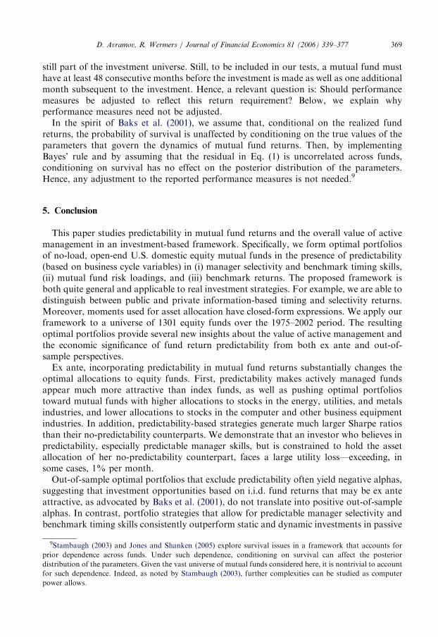
ARTICLE IN PRESSD. Avramov, R. Wermers / Journal of Financial Economics 81 (2006) 339–377 369

still part of the investment universe. Still, to be included in our tests, a mutual fund musthave at least 48 consecutive months before the investment is made as well as one additionalmonth subsequent to the investment. Hence, a relevant question is: Should performancemeasures be adjusted to reflect this return requirement? Below, we explain whyperformance measures need not be adjusted.

In the spirit of Baks et al. (2001), we assume that, conditional on the realized fundreturns, the probability of survival is unaffected by conditioning on the true values of theparameters that govern the dynamics of mutual fund returns. Then, by implementingBayes’ rule and by assuming that the residual in Eq. (1) is uncorrelated across funds,conditioning on survival has no effect on the posterior distribution of the parameters.Hence, any adjustment to the reported performance measures is not needed.9

5. Conclusion

This paper studies predictability in mutual fund returns and the overall value of activemanagement in an investment-based framework. Specifically, we form optimal portfoliosof no-load, open-end U.S. domestic equity mutual funds in the presence of predictability(based on business cycle variables) in (i) manager selectivity and benchmark timing skills,(ii) mutual fund risk loadings, and (iii) benchmark returns. The proposed framework isboth quite general and applicable to real investment strategies. For example, we are able todistinguish between public and private information-based timing and selectivity returns.Moreover, moments used for asset allocation have closed-form expressions. We apply ourframework to a universe of 1301 equity funds over the 1975–2002 period. The resultingoptimal portfolios provide several new insights about the value of active management andthe economic significance of fund return predictability from both ex ante and out-of-sample perspectives.

Ex ante, incorporating predictability in mutual fund returns substantially changes theoptimal allocations to equity funds. First, predictability makes actively managed fundsappear much more attractive than index funds, as well as pushing optimal portfoliostoward mutual funds with higher allocations to stocks in the energy, utilities, and metalsindustries, and lower allocations to stocks in the computer and other business equipmentindustries. In addition, predictability-based strategies generate much larger Sharpe ratiosthan their no-predictability counterparts. We demonstrate that an investor who believes inpredictability, especially predictable manager skills, but is constrained to hold the assetallocation of her no-predictability counterpart, faces a large utility loss—exceeding, insome cases, 1% per month.

Out-of-sample optimal portfolios that exclude predictability often yield negative alphas,suggesting that investment opportunities based on i.i.d. fund returns that may be ex anteattractive, as advocated by Baks et al. (2001), do not translate into positive out-of-samplealphas. In contrast, portfolio strategies that allow for predictable manager selectivity andbenchmark timing skills consistently outperform static and dynamic investments in passive

9Stambaugh (2003) and Jones and Shanken (2005) explore survival issues in a framework that accounts for

prior dependence across funds. Under such dependence, conditioning on survival can affect the posterior

distribution of the parameters. Given the vast universe of mutual funds considered here, it is nontrivial to account

for such dependence. Indeed, as noted by Stambaugh (2003), further complexities can be studied as computer

power allows.

ARTICLE IN PRESSD. Avramov, R. Wermers / Journal of Financial Economics 81 (2006) 339–377370

benchmarks. Specifically, such strategies yield an a of 9.46% and 10.52%/year wheninvestment returns are adjusted using a model with a fixed and with a time-varying marketbeta, respectively. Using the Fama-French (Carhart) benchmarks, the correspondingfigures are 12.89% and 14.84% (8.46% and 11.17%).We show that inter- and intraindustry asset allocation patterns are key to understanding

the source of these superior levels of performance. Specifically, strategies that incorporatetime-varying manager skills outperform their benchmarks by 2–4%/year through theirability to time industries over the business cycle. Moreover, they choose individual fundsthat outperform their industry benchmarks to achieve an additional 3–6%/year. Thesestrategies choose funds that do not differ much in their size, book-to-market, andmomentum styles, based on stock holdings, relative to other strategies that allow for activemanagement skill but disallow predictability in manager skill.We also compare the performance of strategies that incorporate predictability in

managerial skills to that of competing strategies that use past returns and flows: (1) the‘‘hot-hands’’ strategy of Hendricks et al. (1993); (2) the four-factor Carhart (1997) alphastrategy; and, (3) the ‘‘smart money’’ strategy of Zheng (1999). Specifically, we formportfolios that pick the top 10% of funds based on their (1) 12-month compounded priorreturns, (2) alpha with respect to the Fama-French and momentum benchmarks, and (3)positive new cash flows. We show that, unlike our predictability-based strategies, thesecompeting strategies generate insignificant performance relative to the Fama-French andmomentum benchmarks. This suggests that our portfolio strategies are unique, and thatthey outperform optimal strategies that exclude information based on business cyclevariables as well as previously studied strategies that pick funds based on past returnsand flows.Our paper suggests several avenues for future research. First, our framework might be

extended to study optimal portfolios that incorporate predictability based on fund-level ormanager-level variables. The impact of the changing characteristics of stocks held by afund (such as the size, book-to-market, and prior-year return) on the profitability ofoptimal portfolios is also an open question—such characteristics have been widely used inrecent studies of performance evaluation (see, e.g., Daniel et al., 1997). Examining whetherthese characteristics add to the predictability of fund returns may provide further insightsinto active management.

Appendix A. Description of mutual fund database

This part of the appendix describes the database in detail. Our procedure for buildingour database begins with the merged CRSP/Thomson open-end mutual fund databasedescribed by Wermers (2004). This merged database contains monthly fund net returns,self-declared investment objectives (quarterly in Thomson, annually in CRSP), annualturnover and expense ratios, and annual load charges for each shareclass of each fund(from CRSP). Our procedure for classifying and characterizing funds is as follows.

A.1. Investment objectives

We focus on open-end, no-load U.S.-headquartered domestic equity funds. We excludebalanced or flexible funds because we wish to rule out strategies that involve investments innonequity securities, such as U.S. government or corporate bonds.

ARTICLE IN PRESSD. Avramov, R. Wermers / Journal of Financial Economics 81 (2006) 339–377 371

To determine whether a fund qualifies as a domestic equity fund, we proceed throughseveral steps. Then, we determine whether, at the beginning of a given quarter, the fundhas a self-declared investment objective that is consistent with investing almost exclusivelyin domestic equities. In particular, we check the investment objective from the Thomsondatabase, as well as the (somewhat different) investment objective data from the CRSP filesto make a first pass at a classification. In doing so, we verify investment objectives for allshareclasses of a given fund (because the data is missing in some cases from someshareclasses in CRSP). Our approach is to use Thomson investment objectives, which areless precise but rarely missing; CRSP investment objectives are more precise, but the largeproportion of missing data precludes the wholesale use of these data. Nevertheless, we useCRSP objectives to refine, where possible, our inclusion of funds.

Next, we check the name of the fund for words that indicate that it has an objectiveother than domestic equity, such as an international growth fund. This step helps us tocorrect any omissions and/or errors in the Thomson or CRSP investment objectives(i.e., when the investment objective is vague, wrong, or missing). For example, we identifyindex funds both through CRSP investment objectives and through the names of funds,since Thomson does not identify these funds. Finally, we exclude any shareclasses for suchfunds that have a nonzero total load (including front-end and deferred) only during theyear that the total load is nonzero. We exclude all other funds such as balanced funds,international funds, and bond funds.

A.2. Net returns

We obtain monthly net returns from the CRSP mutual fund database. To computethe net return for a given mutual fund in the linked Thomson/CRSP database, weaggregate the net returns on all no-load shareclasses that exist during that month byvalue-weighting the shareclass returns using beginning-of-month total net assets (TNA)for each shareclass. Thus, our monthly returns mimic the returns that would have beenearned by a pro-rata investment across all no-load shareclasses of a given fund. Thisapproach avoids any biases that might result from using only a single shareclass from agiven fund.

When one or more no-load shareclasses has missing returns or total net assetinformation, we aggregate the net returns for remaining shareclasses that have fulldata. Finally, when a missing return is indicated for a fund-month for a shareclassin the CRSP files, the first nonmissing return is discarded to alleviate the CRSP approachof filling in a cumulative return at this date, which would introduce large measurementerrors.

In forming ‘‘hot-hands’’ and ‘‘smart money’’ portfolios of mutual funds as well as inassessing whether the universe of equity funds provides close substitutes to the Fama-French and momentum benchmarks, we include all shareclasses, including those charginga load. In this case, we reconstruct our shareclass-averaged net returns including all no-load and load shareclasses for each fund.

A.3. Turnover and expenses

Like net returns, turnover and expenses are shareclass-averaged for each fund, withrebalancing done when a shareclass disappears or has missing data. Shareclass-specific

ARTICLE IN PRESSD. Avramov, R. Wermers / Journal of Financial Economics 81 (2006) 339–377372

monthly turnover and expenses are derived by dividing the annual numbers (from CRSP)by 12. Weights for shareclass averaging are based on beginning-of-month total net assets(TNA) for the shareclass.

A.4. Flows

Net flows from consumers are estimated with the change in the ratio of total net assetsdivided by the net asset value per share (i.e., the shares outstanding of the fund) during amonth, where the effect of splits during the month are reversed from the end-of-monthshares outstanding. In addition, cash distributions are all assumed to be reinvested,meaning that the growth in shares outstanding are net of all distribution-relatedreinvestments (which are assumed to be 100% reinvested). In other words, reinvesteddistributions, both capital-gain and dividend, are not counted as flows. Before 1991, totalnet assets are available only on a quarterly basis, so monthly flows are estimated bydividing the quarterly number by three.In unreported tests, we compared these estimated flows with the known, actual monthly

flows from a large number of funds from a given major mutual fund family. We find thatthe estimates based on the above procedure are very close to the known actuals for thesefunds (over 100 funds), which provides reassurance that our computation of flows is morebroadly applicable to the universe of funds.

Appendix B. Investments when fund risk loadings and benchmark returns may be predictable

This part of the appendix derives moments for asset allocation under the case in whichfund risk loadings and benchmark returns could be predictable by business cycle variables,but managerial skill is not.

B.1. Prior beliefs

First note that ai1 ¼ 0 in Eq. (1) because skill is assumed to be unpredictable. Part C ofthe appendix relaxes this assumption. The prior on ai0 is

pðai0 jciÞ / ðciÞ�1=2 exp �

1

2ci

ðGi � Gi0Þ0UðGi � Gi0Þ

� �, (8)

where Gi0 ¼ ½ai0; 0; . . . ; 0�0, U ¼ DD0s2=s2a, D is a ðKM þ K þ 1Þ vector whose first element is

one and the rest of the elements are zero, s2a is the degree of belief about managerial skill,and s2 is computed as the cross-sectional average of the sample variance of the residuals inEq. (1). Note that the dogmatic (agnostic) case implies that sa ¼ 0 ð1Þ. The skeptic caseimplies that 0osao1. (In the empirical application, we set sa ¼ 1%.) For the dogmatist,we set ai0 ¼ �

112ðexpenseþ 0:01� turnoverÞ, where expense and turnover are the fund’s

annual average values of reported expense ratio and turnover. For the skeptic andagnostic, we set ai0 ¼ �

112ðexpenseÞ. The prior beliefs about all other parameters in

Eqs. (1)–(3) are taken to be noninformative. Specifically, the prior is proportional toðciÞ

�1jSff j

�ðKþ1Þ=2jSzz:r:f j�ðMþ1Þ=2.

ARTICLE IN PRESSD. Avramov, R. Wermers / Journal of Financial Economics 81 (2006) 339–377 373

B.2. The likelihood function

The sample contains Ti monthly returns of fund i (overall, the investment universecontains N ¼ 1301 no-load, open-end, equity mutual funds) and T monthly observationsof K benchmark returns and M business cycle variables. Fund i enters the sample at time ti

and leaves at time ti þ Ti � 1, following a merger or termination. The fund may remainuntil the end of our sample period, December 2002. Let ri denote the Ti-vector of

excess returns on fund i, let Gi ¼ ½G0ti; . . . ;G0tiþTi�1

�0, where Gt ¼ ½1; f0t; f0t � z0t�1�

0, let

Gi ¼ ½ai0;b0i0;b

0i1�0, let Z ¼ ½z01; . . . ; z

0T �0, let F ¼ ½f 01; . . . ; f

0T �0, let X ¼ ½x00; . . . ;x

0T�1�

0, where

x0 ¼ ½1; z00�0 with z0 being the first observation of the macro predictors, let

V f ¼ ½v0f 1; . . . ; v

0fT �0, let V Z ¼ ½v

0z1; . . . ; v

0zT �0, let Vrz be a T �N matrix whose ith column

contains Ti values of vit when returns on fund i are recorded and T � Ti zeros when such

returns are missing, let AZ ¼ ½az;Az�0, let AF ¼ ½af ;Af �

0, let QGi¼ ITi

� GiðG0iGiÞ

�1G0i, let

QX ¼ IT � X ðX 0X Þ�1X , let W Z ¼ ½X ;V f ;V rz�, and let QZ ¼ IT �W Z W 0ZW Z

� ��1W 0

Z:The processes for fund returns, benchmark returns, and business cycle predictorscharacterized in Eqs. (1)–(3) can be rewritten as ri ¼ GiGi þ vi;F ¼ XAF þ vf , andZ ¼ XAZ þ vz, respectively. Then, the likelihood can be factored as

L /YNi¼1

ðciÞ�Ti=2 exp �

1

2ci

ðr0iQGiri þ ðGi � GiÞ

0G0iGiðGi � GiÞÞ

� �" #

�jSff j�T=2 exp �

1

2tr½S�1ff ðF

0QX F þ ðAF � AF Þ0X 0X ðAF � AF Þ�

� �

�jSzz:r:f j�T=2 exp �

1

2tr½S�1zz:r:f ðZ

0QZZ þ ðx� xÞ0W 0ZW Zðx� xÞ�

� �, ð9Þ

where x ¼ ½A0Z;Szf S�1ff ;SzrC�1�0, C is a diagonal matrix whose ði; iÞth element is ci,

Szz:r:f ¼ Szz � SzrS�1rr Srz � Szf S�1ff Sfz, Sfz is the covariance between vft and vzt, Szz is the

variance of vzt, and Srz is an N �M matrix whose ith row contains the covariance betweenvit and vzt, Gi ¼ ðG

0iGiÞ

�1G0iri; AF ¼ ðX0X Þ�1X 0F ; and x ¼ ðW 0

ZW Z�1W 0

ZZ:

B.3. The predictive moments

The first two moments of the Bayesian predictive distribution displayed in Eq. (7), say attime T, are

EfrTþ1jDT g ¼ ~a0 þ ~bT~A0F xT , (10)

VfrTþ1jDT g ¼ ð1þ dT Þ~bT Sff

~b0T þ AT , (11)

where ~a0 and ~bT are the all-fund versions of ~ai0 and ~biðzT Þ ½~biðzT Þ ¼

~bi0 þ ðIK � z0T Þ~bi1�,

~ai0; ~bi0, and ~bi1 are the first element, the next K elements, and the last KM elementsin the vector ~Gi ¼ ðG

0iGi þ UÞ�1ðG0iri þ UGi0Þ, dT ¼

1T½1þ ðz� zT Þ

0V�1z ðz� zT Þ�, ~AF ¼ AF ,Sff ¼ F 0QX F=ðT � K �M � 2Þ, and AT is a diagonal matrix whose ði; iÞ element is

~ci1ð1þ tr½Sff~Oi�ð1þ dT Þ þ O11

i þ 2½O12i þ O13

i ðIK � zT Þ� ~A0F xT þ tr½ ~A0F xT x0T

~AF~Oi�Þ.

(12)

ARTICLE IN PRESSD. Avramov, R. Wermers / Journal of Financial Economics 81 (2006) 339–377374

In (12), ~ci1 ¼~ci=ðTi � K � KM � 2Þ, ~ci ¼ r0iri þ G0i0UGi0 � ~G0iðG

0iGi þ U Þ ~Gi, ~Oi ¼ O22

i þ

O23i IK � zTð Þ þ IK � z0T

� �O32

i þ IK � z0T� �

O33i IK � zTð Þ, and Omn

i is a partition of ðG0iGi þ

UÞ�1 (based on the partitions of Git ¼ ½1; f0t; f0t � z0t�1�

0Þ given by

ðG0iGi þ UÞ�1 ¼

O11i O12

i O13i

O21i O22

i O23i

O31i O32

i O33i

0B@

1CA. (13)

Appendix C. Investments when skills may be predictable

Here we study the agnostic and skeptic investors. Of course, the dogmatist rules outskill, both fixed and time-varying.

C.1. The agnostic

The agnostic investor allows the data to determine the magnitude of skill, both fixed andtime-varying. Under that assumption of diffuse priors, the Bayesian predictive mean andvariance are given by

EfrTþ1jDT g ¼ ~a0 þ ~a1zT þ~bT~A0F xT , (14)

VfrTþ1jDT g ¼ ð1þ dT Þ~bT Sff

~b0T þ AT , (15)

where the ði; iÞ element of the diagonal matrix AT is given by

~ci2ð1þ tr½Sff~Oi�ð1þ dT Þ þ x0TO

11i xT þ 2xT ½O12

i þ O13i ðIK � zT Þ� ~A

0F xT

þ tr½ ~A0F xT x0T~AF~Oi�Þ, ð16Þ

~ci2 ¼~ci=ðTi � K �M � KM � 2Þ, and the quantities ~ci2 and Omn

i are based upon thepartitions of Git ¼ ½1; zt�1; f

0t; f0t � z0t�1�

0.

C.2. The skeptic

Here, prior beliefs about time-varying skill are informative. To simplify theanalysis we study the case in which risk premia and fund risk loadings are constant.That is, bi1 ¼ 0 and Af ¼ 0 with probability one. When skill varies over time theinvestor’s prior is modeled as if a hypothetical sample of T0 months has been observed.In this sample, there is no manager skill in benchmark timing and stock selectionbased on either public or private information. The mean and variance of fundreturns, benchmark returns, and predictive variables in the hypothetical sample areequal to those in the actual sample. Thus, based on that hypothetical sample, the prior onGi is modeled as

Gijci�N½Gi0;ci½G0i0Gi0�

�1�, (17)

ARTICLE IN PRESSD. Avramov, R. Wermers / Journal of Financial Economics 81 (2006) 339–377 375

where Gi0 ¼ ½ai0; 00; b0i0�

0, ai0 ¼ �112ðexpenseÞ, bi0 ¼ ðf

0f Þ�1ðf 0riÞ � Tiðf0f Þ�1f ai0, and

½G0i0Gi0��1 ¼

1

T0

1þ z0V�1z zþ f 0V�1f f �z0V�1z �f 0V�1f

�V�1z z V�1z 0

�V�1f f 0 V�1f

2664

3775. (18)

To address the choice of T0, we establish an exact link between sa (the skill uncertaintyentertained by Pastor and Stambaugh (2002a,b)) and T0. The link is given by

T0 ¼s2

s2að1þM þ SR2

maxÞ, (19)

where SRmax is the largest attainable Sharpe ratio based on investments in the benchmarksonly (disregarding predictability), M is the number of macroeconomic variables that arepotentially useful in predicting fund returns, and s2 is the cross-fund average of the samplevariance of the residuals in Eq. (1). This exact link gives our prior specification the skilluncertainty interpretation employed by earlier work. To apply our prior specification forthe predictability skeptic investor in the empirical section, we compute s2 and SR2

max, andset sa ¼ 1%. Then, we obtain T0 through Eq. (19).

The derivation of the link displayed in Eq. (19) is presented below. First note that basedon the hypothetical sample, the prior of ai ¼ ½ai0; a0i1�

0 is given by

aijci�N ai;ci

T0

1þ z0V�1z zþ f 0V�1f f �z0V�1z

�V�1z z V�1z

24

35

0@

1A, (20)

where ai ¼ ½�112ðexpenseÞ; 01;M �

0 and 01;M is an M-row vector of ones. Then, we derive theprior variance of ai0 þ a0i1zt�1 using the steps

varðai0 þ a0i1zt�1jci;D0Þ ¼ E½a2i0 þ ai1zt�1z0t�1a0i1 þ 2ai0a0i1zt�1� � a2i0

¼ci

T0ð1þ z0V�1z zþ f 0V�1f f Þ þ

ci

T0trf½V z þ zz0�½V�1z �g

�2ci

T0z0V�1z z

¼ci

T0½1þM þ f 0V�1f f �

¼ci

T0½1þM þ SR2

max�, ð21Þ

where D0 stands for the information in the hypothetical sample, tr denotes the traceoperator, and f 0V�1f f is the square of the maximal admissible Sharpe ratio obtained byinvesting in benchmarks only. The link in Eq. (19) follows by comparing the unconditionalvariance derived in Eq. (21) with that of Pastor and Stambaugh (2002a,b), which is givenby cis

2a=s2.

Next, we form posterior densities by combining the hypothetical prior sample with thenoninformative prior c�1i jSff j

�ðKþ1Þ=2jSzz:r:f j�ðMþ1Þ=2 and the actual data. We then find that

the Bayesian predictive mean and variance are

EfrTþ1jDT g ¼ ~a0 þ ~a1zT þ~bf , (22)

ARTICLE IN PRESSD. Avramov, R. Wermers / Journal of Financial Economics 81 (2006) 339–377376

VfrTþ1jDT g ¼ 1þ1

T�

� �~b ~Vf

~b0 þ AT , (23)

where ~a0; ~a1, and ~b are the all-fund versions of ~ai0; ~ai1, and ~bi, obtained as the first column,the next M columns, and the last K columns of ~Gi ¼ G0iGi þ G0i0Gi0

� ��1G0iri þ ½G

0i0Gi0�Gi0

� �,

AT ði; iÞ ¼ ~ci3 1þ tr½ ~Vf O22i � 1þ

1

T�

� �þ x0TO

11i xT þ 2xTO12

i f þ tr½f f 0O22i �

� �, (24)

T�i ¼ Ti þ T0; T� ¼ T þ T0; ~ci3 ¼ðT�i =TiÞr

0iri � ~G0iðG

0iGi þ G0i0Gi0Þ ~Gi

T�i � K �M � 2,

~Vf ¼T�V f

T� � K � 3,

and the Omni matrices are obtained by partitioning ðG0iGi þ G0i0Gi0Þ

�1.

References

Admati, A., Bhattacharya, S., Pfleiderer, P., Ross, S., 1986. On timing and selectivity. Journal of Finance 41,

715–730.

Ait-Sahalia, Y., Brandt, M., 2001. Variable selection for portfolio choice. Journal of Finance 56, 1297–1351.

Avramov, D., 2002. Stock return predictability and model uncertainty. Journal of Financial Economics 64,

423–458.

Avramov, D., 2004. Stock return predictability and asset pricing models. The Review of Financial Studies 17,

699–738.

Avramov, D., Chordia, T., 2005a. Asset pricing models and financial market anomalies. Review of Financial

Studies, forthcoming.

Avramov, D., Chordia, T., 2005b. Predicting stock returns. Journal of Financial Economics, forthcoming.

Baks, K.P., Metrick, A., Wachter, J., 2001. Should investors avoid all actively managed mutual funds? A study in

Bayesian performance evaluation. Journal of Finance 56, 45–85.

Barberis, N., 2000. Investing for the long run when returns are predictable. Journal of Finance 55, 225–264.

Carhart, M., 1997. On persistence in mutual fund performance. Journal of Finance 52, 57–82.

Chen, J., Hong, H., Huang, M., Kubik, J., 2004. Does fund size erode mutual fund performance? The role of

liquidity and organization. American Economic Review 94, 1276–1302.

Daniel, K., Grinblatt, M., Titman, S., Wermers, R., 1997. Measuring mutual fund performance with

characteristic-based benchmarks. Journal of Finance 52, 1035–1058.

Dybvig, P., Ross, S., 1985. Performance measurement using differential information and a security market line.

Journal of Finance 40, 383–399.

Fama, E., 1996. Multifactor portfolio efficiency and multifactor asset pricing. Journal of Financial and

Quantitative Analysis 31, 441–465.

Fama, E., French, K., 1989. Business conditions and expected returns on stocks and bonds. Journal of Financial

Economics 19, 3–29.

Fama, E., French, K., 1993. Common risk factors in the returns on stocks and bonds. Journal of Financial

Economics 33, 3–56.

Ferson, W., Siegel, A., 2001. The efficient use of conditioning information in portfolios. Journal of Finance 56,

967–982.

Grinblatt, M., Titman, S., 1989. Mutual fund performance: an analysis of quarterly portfolio holdings. Journal of

Business 62, 394–415.

Hansen, L., Richard, S., 1987. The role of conditioning information in deducing testable restrictions implied by

dynamic asset pricing models. Econometrica 55, 587–613.

Hendricks, D., Patel, J., Zeckhauser, R., 1993. Hot hands in mutual funds: the persistence of performance,

1974–88. Journal of Finance 48, 93–130.

Jegadeesh, N., Titman, S., 1993. Returns to buying winners and selling losers: implications for stock market

efficiency. Journal of Finance 48, 65–91.

ARTICLE IN PRESSD. Avramov, R. Wermers / Journal of Financial Economics 81 (2006) 339–377 377

Jones, C.S., Shanken, J., 2005. Mutual fund performance with learning across funds. Journal of Financial

Economics 78, 507–552.

Kandel, S., Stambaugh, R., 1996. On the predictability of stock returns: an asset allocation perspective. Journal of

Finance 51, 385–424.

Keim, D., Stambaugh, R., 1986. Predicting returns in the stock and the bond markets. Journal of Financial

Economics 17, 357–390.

Lehmann, B., Modest, D., 1987. Mutual fund performance evaluation: a comparison of benchmarks and

benchmark comparisons. Journal of Finance 42, 233–265.

Markowitz, H.M., 1952. Portfolio selection. Journal of Finance 7, 77–91.

Markowitz, H.M., 1959. Portfolio Selection: Efficient Diversification of Investments. Yale University Press, New

Haven, CT.

Merton, R.C., 1973. An intertemporal capital asset pricing model. Econometrica 41, 867–887.

Merton, R.C., 1981. On market timing and investment performance Part I: an equilibrium theory of value for

market forecasts. Journal of Business 54, 263–289.

Moskowitz, T., 2000. Discussion: mutual fund performance: an empirical decomposition into stock-picking

talent, style, transactions costs, and expenses. Journal of Finance 55, 1695–1703.

Moskowitz, T., 2003. An analysis of covariance risk and pricing anomalies. Review of Financial Studies 16,

417–457.

Moskowitz, T., Grinblatt, M., 1999. Do industries explain momentum? Journal of Finance 54, 1249–1290.

Pastor, L., 2000. Portfolio selection and asset pricing models. Journal of Finance 55, 179–223.

Pastor, L., Stambaugh, R., 2000. Comparing asset pricing models: an investment perspective. Journal of Financial

Economics 56, 335–381.

Pastor, L., Stambaugh, R., 2002a. Mutual fund performance and seemingly unrelated assets. Journal of Financial

Economics 63, 315–349.

Pastor, L., Stambaugh, R., 2002b. Investing in equity mutual funds. Journal of Financial Economics 63, 351–380.

Roll, R., 1978. Ambiguity when performance is measured by the securities market line. Journal of Finance 33,

1051–1069.

Schwert, G.W., 2003. Anomalies and market efficiency. In: Constantinides, G.M., Harris, M., Stulz, R. (Eds.),

Handbook of Economics and Finance, pp. 937–972.

Shanken, J., 1990. Intertemporal asset pricing: an empirical investigation. Journal of Econometrics 45, 99–120.

Sirri, E., Tufano, P., 1998. Costly search and mutual fund flows. Journal of Finance 53, 1589–1622.

Stambaugh, R.F., 2003. Inference about survivors. Unpublished Working Paper, The Wharton School.

Wermers, R., 1999. Mutual fund herding and the impact on stock prices. Journal of Finance 54, 581–622.

Wermers, R., 2000. Mutual fund performance: an empirical decomposition into stock-picking talent, style,

transactions costs, and expenses. Journal of Finance 55, 1655–1695.

Wermers, R., 2004. Is money really smart? New evidence on the relation between mutual fund flows, manager

behavior, and performance persistence. Unpublished Working Paper, The University of Maryland.

Zellner, A., Chetty, V.K., 1965. Prediction and decision problems in regression models from the Bayesian point of

view. Journal of the American Statistical Association 60, 608–615.

Zheng, L., 1999. Is money smart? A study of mutual fund investors’ fund selection ability. Journal of Finance 54,

901–933.

Further Reading

Jensen, M.C., 1969. Risk, the pricing of capital assets, and the evaluation of investment portfolios. Journal of

Business 42, 167–247.