technological links and predictable returns · 2018-01-10 · technological links and predictable...
TRANSCRIPT

Technological Links and Predictable Returns
Charles M. C. Lee, Stephen Teng Sun, Rongfei Wang, and Ran Zhang**
September 10, 2017
Abstract
This paper finds evidence of return predictability across technology-linked firms.
Employing a classic measure of technological closeness between firms, we show that
the returns of technology-linked firms have strong predictive power for focal firms’
returns. A long-short strategy based on this effect yields monthly alpha of 117 basis
points. This effect is distinct from industry momentum, and is more pronounced for
more innovative firms, firms with higher investor inattention, and firms with higher
costs of arbitrage. We find a similar lead-lag relation between the earnings surprises,
analyst revisions, and innovation-related activities (such as patent and citation counts)
of technology-linked firms. Our results are broadly consistent with sluggish price
adjustment to more nuanced technological news.
JEL classification: G10, G11, G14, O30
Keywords: Technology momentum, stock returns, return predictability, patents,
technological closeness, limited attention, market efficiency
** Corresponding author: Charles M.C. Lee, Joseph McDonald Professor of Accounting, Graduate
School of Business, Stanford University, 655 Knight Way, Stanford, CA 94305-7298; Tel: (650)
721-1295; Fax: (650) 725-9932; Email: [email protected]. Stephen Teng Sun
([email protected]) is Assistant Professor of Economics at the Guanghua School of Management,
Peking University. Rongfei Wang ([email protected]) is a PhD Candidate in Accounting at
the Guanghua School of Management, Peking University. Ran Zhang ([email protected])
is Associate Professor of Accounting at the Guanghua School of Management, Peking University.

1
Technological Links and Predictable Returns
September 10, 2017
Abstract
This paper finds evidence of return predictability across technology-linked firms.
Employing a classic measure of technological closeness between firms, we show that
the returns of technology-linked firms have strong predictive power for focal firms’
returns. A long-short strategy based on this effect yields monthly alpha of 117 basis
points. This effect is distinct from industry momentum, and is more pronounced for
more innovative firms, firms with higher investor inattention, and firms with higher
costs of arbitrage. We find a similar lead-lag relation between the earnings surprises,
analyst revisions, and innovation-related activities (such as patent and citation counts)
of technology-linked firms. Our results are broadly consistent with sluggish price
adjustment to more nuanced technological news.
JEL classification: G10, G11, G14, O30
Keywords: Technology momentum, stock returns, return predictability, patents,
technological closeness, limited attention, market efficiency

2
1. Introduction
The valuation of firms’ technological capabilities is becoming increasingly
important for investors as society becomes more innovation-driven. For many firms
today, technological prowess is an important determinant not only of short-term
profitability but also of long-term survival. At the same time, a firm’s technological
capabilities are notoriously difficult to measure. Moreover, a growing literature
reports that investors do not seem particularly good at valuing these capabilities. For
example, investors tend to misvalue innovation (Cohen, Diether and Malloy, 2013) or
undervalue innovative efficiency and originality (Hirshleifer, Hsu, and Li, 2013,
2017). In this paper, we find that investors also seem to overlook another potentially
important source of technology-related information: recent price-relevant news
affecting other technologically linked firms.
Firms do not conduct its technological research in isolation; frequently, they
interact with each other intensively, leading to an innovation process characterized by
knowledge spillovers (Jaffe, Trajtenberg, and Henderson, 1993). Given the
particular nature of innovation and its ever-growing role in firm behavior and
valuation, it is important that we go beyond firms’ own innovation characteristics and
examine the implications of firms’ interactions in innovation. Firms working on
areas of innovation that substantially overlap with each other could be subject to
similar input or output linkages, which become important transmission channels for
common price shocks (Acemoglu et al., 2012). Firms with similar technologies can
also benefit from the spillover effect of each other’s innovation activity along

3
technological lines (Bloom, Schankerman, and Van Reenen, 2013). Specifically,
firms working on similar technologies may use similar inputs of production, with the
inputs here being broadly interpreted as anything required in the production process,
i.e., valuable human resources, key raw materials, production and management
equipment and structures including Information and Communication Technology
(ICT) or intangible knowledge in production. For example, breakthroughs in
production technology led to dramatic cost reductions in silicon chips, which in turn
greatly impacted on the vitality of the electronics industry that relies on these chips as
a raw material. Similarly, technological progress in touch screen technology today
bodes well for the firms making products that use these touch-screens.
In this paper, we examine how shocks to one firm affect other firms that are
closely related in terms of their technological expertise. While previous studies
document rich asset pricing implications of several types of relationship between
firms, including product market link, customer-supplier link, geographical link, labor
market link, and alliance link (Hou, 2007; Cohen and Frazzini, 2008; Cohen and Lou,
2012; Li, Richardson, and Tuna, 2014; Huang, 2015; Lee, Ma, and Wang, 2015; Li,
2015; Cao, Chordia, and Lin, 2016), relatively little work has been done on the
pricing implications of technological affinity. If investors understand and take into
account the ex ante publicly available technological links, prices of the focal firm
should fully adjust when news about its technology-linked firms arrives at the market.
On the other hand, if investors are slow to understand and/or do not pay enough
attention to the news affecting firms that are closely-aligned in technological space,

4
stock prices of focal firms will exhibit a predictable lag with respect to recent news
affecting its technology-linked peers. Therefore, one asset pricing implication of
investors’ limited processing capability and attention with respect to technological
links is that price movements across linked firms are predictable: specifically, focal
firm prices will adjust with a lag to shocks experienced by linked firms.
To better illustrate our idea that news about one firm could translate into other
firms in the technology space, consider the celebrated “Steve Jobs Patent” (patent
number 7,479,949, with Steve Jobs as Co-inventors), which was granted on January
20, 2009. This patent, titled “Touch screen device, method, and graphical user
interface for determining commands by applying heuristics”, is the core patent of
Apple’s multi-touch technology, which is widely used today in iPhones and iPads.
The granting of this patent was accompanied by extensive media coverage right after
the grant date and in subsequent years.1 During the [t, t+2] window of the patent
grant date, the abnormal return of Apple is 10.56%, which largely accounted for the
firm’s abnormal returns for the entire month of January.2
Although Steve Jobs and Apple are the most direct beneficiaries of this patent
grant, the event is also significant for the broader field of multi-touch technology.
This is because multi-touch technology has wide applicability to many products
beyond iPhones and iPads.3 For example, touch screens can be used in products
1 For example: http://www.dailytech.com/Apple+Awarded+MultiTouch+Patent/article14073.htm. The
wide influence of the “Steve Jobs Patent” is also reflected in the enormous number of forward citations:
as of August 31, 2017, it has been cited more than 1,000 times, according to the google patent website.
https://patents.google.com/patent/US7479949B2/. 2 The 3-day abnormal return is defined as 3-day cumulative market adjusted return, where the market
return is the CRSP value-weighted average return. 3 As the title suggests, multi-touch technology allows two or more fingers to be used on the
touchscreen, and this enables devices to recognize and respond to more than one touch at the same time.
5
such as televisions, interactive screens, and ATMs. This technology also has
application in contexts as wide as in-car instrument panels, intelligent home
appliances, hospitality counters, among others. According to Research and Markets,
a market research company, the global market for multi-touch screen alone was
valued at $6 billion in 2016, and is projected to reach $16 billion by 2023.4
Therefore, while the granting of this patent confers some monopoly power upon
Apple, it also is an endorsement of the potential value and the technological feasibility
of multi-touch technology as a whole. It seems likely that other firms with similar
technological expertise will also benefit from this new information.
In Appendix Table A1, we report the returns for a portfolio of firms that are most
closely linked to Apple in terms of their technology, in the months surrounding the
approval of the Steve Jobs patent. Market-adjusted return (MAR) is defined as raw
monthly return minus CRSP value-weighted monthly return, and all stocks within a
given portfolio are weighted by a measure of technology closeness following Jaffe
(1986). For the month of the patent grant (January 2009), the full-sample MAR is
6.43% (t=6.10). In the subsequent month (February), the full-sample MAR is 2.67%
(t=4.71). These results suggest some contemporaneous stock comovement, as well
as some lead-lag effect. Interestingly, the effect of the contemporaneous
comovement is stronger for firms in the same 2-digit industry as Apple, while the
lead-lag return predictability is more pronounced for firms in different industries. In
fact, we find that technological proximity is directly related to the intensity of these
The multi-touch technology greatly expands the range of functionality that devices can support. For
instance, pinch to zoom is a classic function that works with multi-touch technology. 4 https://www.thestreet.com/story/14257336/1/.
6
results – both contemporaneous comovement and lead-lag return predictability are
stronger in the portfolio with the closest technology-link. These anecdotal findings
suggest that the pricing implications are stronger for firms with closer technological
ties.5 The Steve Jobs example demonstrates that technological affinity, an idea that
was first documented in Jaffe (1986), can capture an important dimension of
inter-firm relationship. To the extent that investors do not immediately recognize the
price relevance of this information, we would expect a diffused price adjustment
process along the lines of these technological links.
To test for the return predictability of technology-linked firms more generally,
we implement the following portfolio strategy. For each focal firm i, we calculate
the weighted return of a portfolio of firms that share similar technology as the focal
firm, 𝑇𝐸𝐶𝐻𝑅𝐸𝑇𝑖 = ∑ 𝑇𝐸𝐶𝐻𝑖𝑗 ∙ 𝑅𝐸𝑇𝑗𝑗≠𝑖 / ∑ 𝑇𝐸𝐶𝐻𝑖𝑗𝑗≠𝑖 where 𝑅𝐸𝑇𝑗 is the return of
firm j and 𝑇𝐸𝐶𝐻𝑖𝑗 measures the degree of technology closeness between firm i and j.
Specifically, we adopt the classic approach first pioneered in Jaffe (1986) and
developed in Bloom, Schankerman, and Van Reenen (2013) to calculate 𝑇𝐸𝐶𝐻𝑖𝑗,
which exploits firm-level data on patent distribution out of 427 different technology
classes to locate firms in a multidimensional technology space.
We then sort focal firms into decile portfolios based on lagged returns of their
technology-linked firms, and find strong evidence that lagged returns of those
technology-linked firms have significant return predictability for focal firms.
Specifically, a portfolio that goes long in those focal firms whose technology-linked
5 This results also indicate that it is important to use the degree of technology closeness as weights to
calculate technology-linked returns (TECHRET).
7
firms performed best in the prior month and goes short in those focal firms whose
technology-linked firms performed worst in the prior month, yields an equal-weighted
return of 117 basis points (t=5.47) per month. For the analogous value-weighted
portfolio, the returns are 69 basis points per month (t=3.19). We refer to this return
predictability as “technology momentum”. In subsequent tests, we show these return
prediction results are robust to a variety of controls, including size, book-to-market,
gross profitability, asset growth, R&D intensity, short-term reversal and medium-term
price momentum variables.
It is natural for firms in the same industry to share similar technologies, so
perhaps the return predictability we document is a rediscovery of the well-known
industry momentum effect (Moskowitz and Grinblatt, 1999; Hou, 2007). On the
other hand, prior studies report that while firms’ technology space has some overlap
with their product market space, firms in distinct product markets or industries also
often invest in similar technologies.6 Empirically, we also find that firms in the
closest technology-linked cohorts can come from many different industries.7
To formally test the prediction that the technology momentum effect that we
6 For example, Bloom, Schankerman, and Van Reenen (2013) document that while IBM, Apple,
Motorola, and Intel are all close in technology space, as demonstrated in their patenting activity and
joint research partnerships, but only IBM and Apple compete in the same PC market and only Motorola
and Intel compete in the semiconductor market. They also document firms competing in the same
industry (or more specifically, the same product market) may invest R&D in distinct technologies.
For instance, Gillette and Valance both compete in batteries but Gillette does R&D mainly in personal
care products while Valance developed a new phosphate technology for lithium ion batteries. 7 In our tests, an average (median) patent technology class contains firms from 10 (10) different
2-digit SIC industries and 31 (26) different 4-digit SIC industries. The average HHI concentration
ratio in a patent technology class by different 2-digit (4-digit) industry is 0.37 (0.21), showing that
various industries indeed secure patents in the same technology class. An HHI concentration ratio
close to 1 in our case means the majority of patents in one technology class comes from one industry
while a smaller ratio means patents are more evenly distributed among different industries in a given
technology class. In comparison, the HHI concentration ratio based on sales for an average 3-digit
SIC industry in Hou and Robinson (2006) is 0.54.

8
documented is not driven by the industry momentum effect identified by Moskowitz
and Grinblatt (1999), we incorporate past and current industry returns in our tests and
find that the technology-linked results are even stronger in the presence of industry
controls. In further tests, we also control for supplier and customer returns, and
pseudo-conglomerate returns, and find that our main results continue to hold.
Overall, these tests show that the technology momentum that we documented is
distinct from return momentum arising from industry links, customer-supplier links,
and standalone-conglomerate firm links.
To establish the robustness of this return predictability result, we conduct a series
of additional tests. First, we examine the predictive relation in sample sub-periods.
Dividing the full sample into four sub-periods, we find a clear and robust lead-lag
return relation in every sub-period. Next, we examine the sensitivity of our results to
the age of the technological closeness measure. Specifically we compute the
closeness measure based on patent issuance data that is available in year t, t-1, t-2, and
t-3. Our results show that measures of TECHRET relying on lagged one-, two-, and
even three-year technology closeness data still significantly predict focal firm returns,
although the predictive power decreases as the technology mapping becomes more
stale. Evidently, investors can form trading strategies like ours even with relatively
old measures of technological closeness.
Finally, we perturb the length of the return estimation and holding periods.
Following Moskowitz and Greenblatt (1999), we use various (L, H) strategies,
whereby the technology momentum portfolios are formed on L-month lagged returns,

9
held for H months, and rebalanced monthly. We examine various different lags (L =
1, 3, 6, and 12) and a variety of different holding periods (H = 1, 6, 12, 24, 36). We
find that the profitability of shorter-term strategies is not sensitive to the length of
ranking period L. The equal-weighted raw monthly return for (1,1) strategy and
(12,1) strategy is 1.17% and 1.11%, respectively. We also find that the profits decay
monotonically and diminish to be insignificant in the longer holding period H.
Specifically, we observe no sign of any return reversal in the longer period, indicating
that the return predictability of technology momentum cannot be explained by
investors’ overreaction.
Having established the robustness of the main result, we then conduct a series of
cross-sectional tests to shed light on how this result varies across different firms and
types of news. Ex ante, we posit that the magnitude of the delayed price reaction
will be an increasing function of: (a) the relevance of technology-linked firm news to
the focal firm, (b) the extent to which investors are inattentive, and (c) the relative
costs of arbitrage.
Specifically, we expect a stronger effect for focal firms that are more
innovation-driven (as measured by the size of their R&D spending and patent-related
activities, both scaled by book equity). If the technology momentum we document
represents a market inefficiency driven by investors’ limited attention and information
processing capacity, we should find a stronger effect for firms that investors are more
likely to overlook. To test this hypothesis, we use firm size, analyst coverage, and
institutional ownership as proxies for investor attention. Finally, if the return

10
predictability reflects mispricing, we would expect to see a greater effect in situations
where arbitrage costs are higher (firms with greater idiosyncratic volatility, or in the
case of bad news).8
Our test results support all these conjectures. We find strong evidence that the
technology-linked momentum effect is more pronounced when the focal firm is:
smaller, has fewer analysts covering them, has lower institutional ownership, and
exhibits higher arbitrage costs (proxied by idiosyncratic volatility and bad news).
The effect is also much stronger (more than doubled) for firms with higher than
median R&D spending and patent-related activities. These results further support
the view that technology momentum is a mispricing phenomenon driven by investors’
limited attention, valuation uncertainty, and arbitrage costs.
Finally, we conduct a series of tests designed to establish the fundamental nature
of the lead-lag pattern observed in returns. An alternative to the mispricing
explanation is that firms with similar technology are exposed to similar risk factors,
and that variations in these risk factors are driving the lead-lag return pattern. It is
not easy to think of examples of risk factors that might behave in ways that give rise
to these patterns. Nevertheless, a risk-based argument is difficult to rule out using
evidence based on stock return correlations alone.
In our final set of tests, we turn to measures of real activity and show that
technological linkages are helpful in identifying lead-lag correlation in the operating
performance as well as the innovation-related activities of tech-linked firms.
8 Prior studies suggest bad news tend to be incorporated into price more slowly (Hong, Lim, and Stein,
2000), either because investors are more reluctant to sell their losers, or because short-selling is more
costly to implement (Beneish, Lee, and Nichols, 2015).

11
Specifically, we find that the lagged earnings surprises (SUEs) of the
technology-linked firms are strong predictors of focal firm earnings surprises (SUEs),
even after controlling SUEs of the focal firm from the last four quarters. In fact, the
SUEs of the tech-linked firms have predictive power for the focal firm’s SUE over the
next four quarters. We observe a similar pattern in analyst forecast revisions
(FREV). Specifically, we find that, after including a host of control variables, lagged
FREVs of the tech-linked firms have strong predictive power for the FREV of the
focal firm. These earnings-based results strongly suggest that the return patterns we
documented earlier have their root in lead-lag patterns in firm fundamentals.
Furthermore, we find a similar lead-lag pattern in two important
innovation-related activities: the patent and citation counts. Specifically, we show
that the average number of patents granted in a given year to a portfolio of
technology-linked firms (where each peer firm is weighted by its pairwise closeness
to the focal firm) has significant predictive power for the patent applications of the
focal firm in the subsequent year. Similarly, the citation counts of technology-linked
peers (the number of forward life-time citations received by patents granted in a given
year) is a significant predictor of the citation counts of the focal firm. These results
are robust to the inclusion of a myriad of control variables, including year and
industry (or firm) fixed effects. Taken together, the patent and citation counts results
document a strong “innovation spillover” effect along technology-linked firms, which
lends further credence to the sluggish price adjustment hypothesis.
The remainder of the paper is organized as follows. Section 2 lays out the

12
background for the setting we examine in the paper. Section 3 describes the data and
variables. Section 4 provides our main results on technology momentum. Section
5 conducts more extensive robustness tests while Section 6 examines the mechanisms
in more detail. Section 7 explores the real effects of the technological link and
Section 8 concludes.
2. Background
Our paper is broadly related to several strands of literature. Firstly, there is a
rich literature documenting the patterns and consequences of investors’ limited
attention to information with substantial value implications. Theoretical works
starting with Merton (1987) examine the effect of investor inattention in security
prices, followed by later studies including Hong and Stein (1999), Hirshleifer and
Teoh (2003), and Peng and Xiong (2006). The general message from these models
is that delayed information recognition due to investors’ limited attention can give rise
to return predictability, beyond explanations by traditional asset pricing models. A
growing empirical literature is lending substantial support for these models’
predictions.9 In particular, Cohen and Frazzini (2008) find investors pay limited
attention to the performance of focal firm’s economically linked firms, i.e., the
customer firms. Consequently, focal firm’s stock price does not immediately
incorporate news involving linked firms, generating predictable future price
movement. We here study a more nuanced but nevertheless important link between
9 Exemplary works include Huberman and Regev (2001), Barber and Odean (2007), DellaVigna and
Pollet (2009), Hou (2007), Menzly and Ozbas (2010), and Hong, Torous and Valkanov (2007).
13
firms: their distance in technology space. Given limited investor attention, we posit
the value implications of this link will only be fully priced gradually over time,
particularly for firms that are more costly to arbitrage.10
Secondly, our work relates to research that examines investors’ limited
information processing capacity and its ramifications. Investors’ biased
interpretation of information could lead to a significant delay in the impounding of
information into asset prices. Tversky and Kahneman (1974) and Daniel, Hirshleifer,
and Subrahmanyam (1998), among others, show that this bias could stem from
investors overweighting their own prior beliefs and underweighting observable public
signals. Numerous recent empirical works lend support to this view. For example,
investors under-react to public announcements of corporate events (Kadiyala and Rau,
2004), stock splits (Ikenberry and Ramnath, 2002), and goodwill write-offs (Hirschey
and Richardson, 2003). Some of this work shows industry peer firms’ stock return
portends the focal firm’s stock return. For instance, Hou (2007) finds a lead-lag
pattern between weekly returns of large firms and small firms from the same industry,
and Jiang, Qian and Yao (2016) find industry leaders’ R&D growth could have
predictability for stock returns of other firms in the same industry, due to R&D
spillover effects. Our study of technology-linked momentum is a context where
investors are subject to limited information processing capacity along the
technological links, which often transcend industry links.
Thirdly, our work joins a burgeoning literature that studies the asset pricing
10 We use idiosyncratic volatility as a proxy for cross-sectional differences in arbitrage costs. Firms
with greater idiosyncratic volatility are generally more costly for investors to trade (see Baker and
Wurgler, 2006).

14
implications of firms’ innovation-related activities. Existing works find various
aspects of firm’s innovation activity, such as R&D intensity (Chan, Lakonishok, and
Sougiannis, 2001), R&D growth (Penman and Zhang, 2002; Eberhart, Maxwell, and
Siddique, 2004; Lev, Sarath, and Sougiannis, 2005), patent citations (Gu, 2005;
Matolcsy and Wyatt, 2008), and more recently, innovative efficiency (Hirshleifer, Li
and Hsu, 2013) and innovative originality (Hirshleifer, Li and Hsu, 2017) have strong
predictability for its future operating performance and stock return. Our work is
distinct from the existing literature in that we study the effect innovations by
technologically related peer firms, rather than innovations at the focal firm itself.
Our work is inspired by Bloom, Schankerman, and Van Reenen (2013), who
demonstrate that a firm’s technology space and product market space provide two
distinct inter-firm networks, as two firms in different product market industries could
produce patent in the same technology class and share similar innovative
knowledge.11 Utilizing the measure of technology closeness originally from Jaffe
(1986), they demonstrate the effect of peer firms’ R&D spending could be
decomposed into technology spillover effect (on technology space) and product
market stealing effect (on product market space). Our paper also makes use of this
approach to parametrize the distance between two firms in technology space and
complements the literature that has focused exclusively on the product market space.
In this dimension, our paper belongs to a growing accounting and finance literature 11 It is useful to note that the Bloom, Schankerman, and Van Reenen (2013) capture the effects of
concurrent R&D spending, our return prediction captures the information contained in other tech peers’
both existing and new knowledge stock. For example, stock return of a technology peer firm could
reflect investor valuation of new patent, or about valuation change to certain technology embedded in
existing patents due to news reflecting potential new usage or news about new innovations that will
make the existing technology obsolete.

15
that studies the wide implications of previously understudied firms’ technological link,
for example, corporate cash-holding (Qiu and Wan, 2014), M&A (Bena and Li, 2014),
bankruptcy (Qiu, Wang and Wang, 2016), strategic alliances (Li, Qiu and Wang, 2017)
and analysts coverage and forecast (Tan, Wang and Yao, 2016). Particularly relevant
to our work, Tan, Wang and Yao (2016) provide strong evidence that an information
spillover effect exists between two technologically related firms and it has substantial
implications for analyst coverage.
Lastly, our work is related to a concurrent working paper by Bekkerman and
Khimich (2017; hereafter BK) that also examines the pricing implications of firms’
technological link. We became aware of BK’s work only as we were wrapping up
our own. The motivating research question and main results of the two studies are
similar. However, our paper differs from BK in several important respects. First,
BK apply textual analysis to patent documents to determine technological affinity,
while our paper measures pairwise distance using patent class distribution (Jaffe,
1986).12 One advantage of our measure is that it measures the degree of technology
closeness between firms, providing an economically meaningful weighting scheme to
construct a weighted-average return of technology-linked firms. Second, due to
more stringent data requirements, BK only examine stock returns from 1997 onward,
while our approach enables us to study a much longer time period (from 1963
onward). Finally, we provide an extensive set of test results that document a lead-lag
12 The Jaffe (1986) approach is gaining wide acceptance in economics. A growing empirical
literature in accounting and finance has also utilized the this approach to measure the distance between
firms’ in technology space (such as Bena and Li, 2014; Qiu and Wan, 2015; Qiu, Wang and Wang,
2016; Li, Qiu, and Wang, 2016; Tan, Wang, and Yao, 2016). None of these studies focus on the issue
of lead-lag patterns in returns.

16
relationship in the fundamentals of technology-linked firms (i.e., unexpected earnings,
analyst forecast revisions, patent and citation counts). Overall, the two papers
corroborate well with each other, and provide complementary evidence that firms’
technological links contain valuable information that market prices only fully
incorporate gradually over time.
3. Data and Variables
The main data set used in this study is the Google patent data generously
provided by Kogan et al. (2017).13 Specifically, Kogan et al. (2017) use Optical
Character Recognition (OCR) technology and a number of textual analysis algorithms
to extract relevant information from the patent document, and then map the identified
assignees to the Center for Research in Security Prices (CRSP) unique identifiers
(PERMNO). This dataset covers 1.9 million CRSP matched patents granted by the
US Patent and Trademark Office (USPTO) from 1926 to 2010.14 We extract CRSP
matched patent information from the Google patent data to construct our
technology-linked variables.
Since we focus on the stock market implication for the patent information, it is
important to identify patents that are publicly available to investors to avoid
look-ahead bias. In particular, there are two important time points for each patent:
the application date and the grant date. The application date is the date that the
13 The Google patent data are available at: https://iu.app.box.com/patents. 14 The Google patent data has a more extensive coverage than the NBER patent data developed by Hall,
Jaffe, and Trajtenberg (2001). For example, during the same period covered by the NBER patent data
(1976-2006), the Google patent data adds an average of 2,187 patents per year to the NBER patent data
and corrects some errors.

17
inventors apply for a new patent to the USPTO, the grant date is the date that the
patent gets formally issued by the USPTO, and the lag between the two dates is on
average two to three years. Unless there is a federal holiday, the USPTO issues
patents every Tuesday, and its publication, Official Gazette, lists detail information of
the patents granted on that day.15 Thus the investors are able to get the patent
information freely from the patent offices on the grant date.16 Examining abnormal
stock turnover around patent grant date, Kogan et al. (2017) provide evidence that
patent grant conveys important information to the market and is reflected in the stock
price. Therefore, we use the grant date as our key time point to identify the patent
information.
Our main sample consists of firms in the intersection of the Google patent data,
CRSP and COMPUSTAT. We focus the analysis on common stocks (CRSP share
codes 10 and 11) and exclude financial firms with one-digit SIC codes of six. To
insure that the relevant accounting and patent information is publicly known to
investors in the market, we impose at least a six-month gap between fiscal-year end
month and stock returns in our stock return tests. Specifically, we first match the
Google patent data for grant year t with COMPUSTAT accounting data for the same
fiscal year t, and then match to CRSP stock returns data from July year t+1 to June
year t+2, as in Fama and French (1992). We require firms to have non-missing
15 The USPTO patent information is available at: https://www.uspto.gov/patent. 16 We note that after the American Inventors Protection Act (AIPA), which came into effect on
November 30, 2000, the USPTO began publishing patent applications 18 months after the application
date. For patents that were filed after November 30, 2000, the market had full knowledge of the
patent at the publication date (which is 18 months after the application date) or the grant date,
depending on which is earlier. In contrast, for the patents filed before November 30, 2000, the grant
date was the earliest time for the market to know the patent.

18
market equity and SIC classification code from CRSP, and non-negative book equity
data at the end of previous fiscal year from COMPUSTAT. We further restrict our
sample to firms that have at least one patent granted in the rolling-window of past five
years.17 In order to reduce the impact of micro-cap stocks, we exclude from our
sample stocks that are priced below one dollar a share at the beginning of the holding
period. 18 Moreover, we employ the return correction approach suggested in
Shumway (1997) for the delisting bias, though these adjustments have no effect on
our results.
In addition to stock returns, we obtain institutional holdings data from the
Thomson Reuters 13F dataset, and analyst forecast data from Institutional Brokers’
Estimate System (IBES) unadjusted files. Specifically, in each month we get most
recent mean consensus forecasts as well as the analyst coverage number immediately
prior to the portfolio formation date. Following Jegadeesh et al. (2004), analyst
forecast revision is defined as the change of one-year-ahead earnings consensus
forecasts for the same fiscal year in a given month, scaled by the beginning price of
the month.
We measure technology-linked return (TECHRET) as the average monthly return
of technology-linked firms in the technology space weighted by pairwise technology
closeness, which is determined on the basis of 427 different technology classes
defined by USPTO for all patents. Formally, technology-linked return for firm i and 17 In the robustness tests (Panel A, Online Appendix Table A.1), we further require the sample firms to
have at least two or three years with granted patents in the rolling-window of past five years, and our
results are robust with this alteration. 18 In the robustness tests (Panel B, Online Appendix Table A.1), we exclude stocks with price below
five dollars a share or market capitalizations below the 10th percentile of NYSE stocks in our analysis,
and find results unchanged.

19
month t is defined as:
𝑇𝐸𝐶𝐻𝑅𝐸𝑇𝑖𝑡 = ∑ 𝑇𝐸𝐶𝐻𝑖𝑗 ∙ 𝑅𝐸𝑇𝑗𝑘𝑗≠𝑖
/ ∑ 𝑇𝐸𝐶𝐻𝑖𝑗𝑗≠𝑖
where k ={1, 3, 6, 12} represents the number of past month returns of
technology-linked firm j. Unless otherwise noted, we use k = 1 to construct our
main variable throughout the paper. We also take k = 3, 6, 12 in our robustness tests.
Following Jaffe (1986) and Bloom, Schankerman, and Van Reenen (2013), 𝑇𝐸𝐶𝐻𝑖𝑗
is the technology closeness defined as the uncentered correlation between all pairs,
𝑇𝐸𝐶𝐻𝑖𝑗 =(𝑇𝑖𝑇𝑗
′)
(𝑇𝑖𝑇𝑖′)1/2(𝑇𝑗𝑇𝑗
′)1/2
where 𝑇𝑖 = (𝑠1, 𝑠2, … , 𝑠𝜏, … , 𝑠427) is the vector of firm i’s technology activity of 427
elements and the τth element 𝑠𝜏 is the average share of number of patents in USPTO
technology class τ out of the firm i’s total number of patents over the rolling past five
years. Technology closeness ranges between zero and one, depending on the degree
of overlap in technology space, and is symmetric in firm ordering (i.e., 𝑇𝐸𝐶𝐻𝑖𝑗 =
𝑇𝐸𝐶𝐻𝑗𝑖 ). Note that by construction the TECH essentially acts as a weight in
calculating the average stock return of technology-linked firms and is biased toward
firms more technologically close to the focal firm (i.e., firms more adjacent to the
focal firm in technology space is given higher weights). TECH is calculated at the
end of each year t based on patent grant date that is publicly available, and then
mapped to the return data from July year t+1 to June year t+2. Other variables are
defined in Appendix Table A2.
The final sample consists of 561,989 firm-month observations spanning July
1963 to June 2012 (i.e., 588 months). Panel A of Table 1 presents the descriptive
20
statistics of sample firms. The number of firms varies from a low of 189 firms in
July 1963 and a high of 1,363 firms in June 2012. The sample firms cover almost 53%
of the CRSP common stock universe in terms of market capitalization. This is
unsurprising since we only include the sample firms with at least one patent granted in
the past five years. We note that the average number of linked firms in the
technology space is 280, and the pairwise technology closeness (TECH) has the
average of 0.11 and standard deviation of 0.16, indicating that the technological link
is quite pervasive and sparse.19 Panel A of Table 1 reports summary statistics for our
key variables. The average technology-linked return (TECHRET) is 0.01. The
distribution pattern is quite similar to industry momentum return (INDRET), and less
volatile than firm past one-month return (REV).
In Panel B of Table 1, several correlation coefficients are noteworthy. The
Pearson correlation between TECHRETt-1 and RETt is 0.028, providing raw evidence
for the lead-lag effect along the technological link. Although TECHRETt-1 exhibits
trivial correlations with a bunch of traditional return predictors (i.e., size,
book-to-market, gross profitability, asset growth, R&D intensity), it is considerably
positively correlated with industry momentum return (INDRETt-1), past one-month
return (REV) and medium-term momentum (MOM) (Pearson correlations are 0.203
for INDRETt-1, 0.124 for REV, and 0.031 for MOM). In the subsequent analysis, we
show the return predictability of TECHRETt-1 remains after controlling for other
variables under various settings.
19 In the robustness tests (Panel C, Online Appendix Table A.1), we only include sample firms of
which the technology-linked firms have TECH larger than 0.01 or rank in the top 50 in terms of TECH,
our main results are unchanged.

21
4. Empirical Results
4.1. Portfolio tests
Table 2 shows the basic results of our paper. At the beginning of each month,
we sort all firms into deciles based on the return of their technology-linked portfolios
in the previous month. The decile portfolios are then rebalanced at the beginning of
each month to maintain either equal or value weights. The bottom lines show the
returns of a zero-cost portfolio that hold the top 10% high technology-linked firm
return stocks and sells short the bottom 10% low technology-linked firm return
stocks.
In Table 2, we find strong evidence consistent with technology-linked firm
returns predict focal firm returns. Specifically, taking the strategy of going long in
firms whose technology-linked firms performed best in the prior months and selling
short those firms whose technology-linked firms performed worst (L/S), yields
equal-weighted returns of 117 basis points per month (t = 5.47), or roughly 14.1% per
year. The corresponding value-weighted returns from the L/S portfolio are 69 basis
points per month (t = 3.19), or about 8.3% per year. In the next five columns, we
control for other known return determinants. The technology-momentum strategy
delivers CAPM abnormal returns of 1.22% (0.74%) per month for the equal (value)
weighted portfolios. The strategy delivers Fama and French (1993) abnormal returns
of 1.26% (0.80%) per month for the equal (value) weighted portfolios. Adjusting
returns for the stock’s own price momentum by augmenting the factor model with
22
Carhart’s (1997) momentum factor has the only negative but negligible effect on the
results. Subsequent to the portfolio formation, the baseline long-short portfolio
earns an abnormal return of 1.08% (0.65%) per months for equal (value) weighted
portfolios. Lastly, we adjust returns using the Fama and French (2015) five-factor
model and using the five-factor model plus the momentum factor. Those
adjustments have little effect on the results: subsequent to the portfolio formation, the
baseline zero-cost portfolio earns abnormal returns of 1.37% (0.86%) and 1.21%
(0.73%) for equal (value) weighted portfolios. The results show that after
controlling for common risk factors, high (low) technology-momentum stocks earn
high (low) subsequent (risk-adjusted) returns.20
4.2. Regression results
In this section, we formally test our hypothesis in a regression framework,
controlling for other determinants of firm return and isolate the marginal effect of our
main variable, lagged technology-linked returns. Specifically, in Table 3, we
conduct forecasting regressions of focal firm returns using Fama and MacBeth (1973)
regressions. The dependent variable in columns 1-3 is the focal firm return in month
t (RETt). The independent variable of interest is the return of the focal firm’s
technology-linked firms in month t-1 (TECHRETt-1). We also include the
20 In Panel D of Online Appendix Table A.1, we show the portfolio results using alternative weighting
schemes. Specifically, for the equal-weighted scheme (i.e., constructing TECHRET by giving all
technology-linked firms equal weights), the long-short portfolio earns raw returns of 1.07% (0.64%)
per month for equal (value) weighted portfolios. For the value-weighted scheme (i.e., weighting
returns of technology-linked firms by their market capitalization), the long-short portfolio return
decrease to 0.39% (0.36%) per month for equal (value) weighted portfolios. These portfolio returns
are smaller than the TECH-weighted (i.e., weighting returns of technology-linked firms by the degree
of technology closeness to focal firms) baseline results in Table 2, supporting the value of technology
closeness (TECH) weighting scheme.
23
value-weighted industry return of the focal firm in month t-1 (INDRETt-1) as an
independent variable, following Cohen and Lou (2012) and Moskowitz and Grinblatt
(1999). Other control variables include lagged size, book-to-market, gross
profitability, asset growth, R&D intensity. Lastly, we include REV, a short-term
return reversal variable, defined as the focal firm’s stock return in month t-1, to
control for the short term reversal effect of Jegadeesh and Titman (1993), and MOM, a
medium-term price momentum variable, defined as the focal firm’s stock return for
the last 12 months except for the past one month, to control for the momentum effect
of Chan, Jegadeesh, and Lakonishok (1996). Cross-sectional regressions are run
every calendar month and the time-series standard errors are Newey-West adjusted
(up to 12 lags) for heteroskedasticity and autocorrelation.
Table 3 column 1-3 report the basic results. Consistent with the portfolio
results, TECHRETt-1 is a strong predictor of next month’s technology-linked focal
firm return in all three specifications. Specifically, before controlling for any other
variables, the coefficient of TECHRETt-1 in column 1 is 0.643 with a t-statistic of 4.18,
indicating that the average monthly return spread of the focal firms in the top and
bottom technology-linked return deciles is 64.3 basis point. In column 2, we include
size, book-to-market, gross profitability, asset growth, R&D intensity, reversal, and
momentum as control variables. The magnitude and significance of the coefficient
of TECHRETt-1 are almost the same as in column 1. In column 3, we further include
lagged industry return as a control variable. Both the magnitude and the significance
of the coefficient of TECHRETt-1 are getting even more pronounced to predict focal

24
firm’s return for month t after adding the industry momentum control variable, which
indicates that the technology momentum effect we documented cannot be explained
by the industry momentum effect documented by Hou (2007).
To better distinguish our technology-momentum effect from the previously
known industry momentum effect, we further report results of taking the
industry-adjusted return (calculated as the difference between a focal firm’s return this
month and its contemporaneous industry return) instead of the raw return as a
dependent variable. By subtracting the industry return from focal firm return, we
purge out stock return continuation that arises from industry wide return
auto-correlations. Column 4 of Table 3 indicates that, even after subtracting this
industry-wide information, TECHRETt-1 remains a strong predictor of focal firms’
returns next month. The magnitude and significance of the coefficient for
TECHRETt-1 are virtually the same when we use industry-adjusted returns. Finally,
consistent with the prior literature (Cohen and Lou, 2012), if the part of predictable
returns of focal firms is solely attributable to delayed information processing, rather
than industry-wide return continuation, we should see past industry returns have no
predictive power for (RETt-INDRETt). Consistent with this prediction, we find that
the coefficient on past industry returns, INDRETt-1, is indistinguishable from zero in
column 4. The coefficients for the control variables are also consistent with prior
literature: size, asset growth, and reversal variable are significantly negative related to
future returns, while the coefficient of book-to-market, gross profitability, R&D
intensity, and momentum are positive.
25
We further control for supplier and customer returns (Menzly and Ozbas, 2010),
pseudo-conglomerate returns (Cohen and Lou, 2012), and stock turnover in Table 4.
The results confirm the return predictability along the supply-chain as well as in the
complicated firms, and low turnover stocks require higher future returns. We note
that the magnitude and significance of the coefficient for TECHRETt-1 are
qualitatively the same as our main results, indicating that the information diffused
along the technological link cannot be explained by the information shocks from
supply-chain, business segment, or the illiquidity of stocks.
5. Other Robustness Tests
5.1. Technology-linked return predictability across time
In Online Appendix Table A.2, we examine whether the return predictability
power of technology-linked firms varies across time. We divide our full sample
periods into 1963-1979, 1980-1989, 1990-1999, and 2000-2012. We then exactly
repeat our baseline analysis from Table 3 for each subperiod. Our results hold up
well to this time disaggregation. The coefficients of TECHRETt-1 are all positive and
statistically significant after controlling for various return determinants.
In fact, the only surprise in Online Appendix Table A.2 is that there appears to be
little industry momentum in the last subperiod, which runs from 2000-2012. The
coefficient of INDRETt-1 is not significant for 2000-2012, while it is significant for the
first three subperiods. It is hard to say whether this just reflects noise in a short
sample or the fact that more arbitrageurs have caught on to the industry momentum

26
effects and are beginning to drive them out of existence. In any case, what is
noteworthy from our perspective is that though the average degree of industry
momentum may be declining over time, the technology momentum that we
documented have been robust across four periods.
5.2. Persistence of technology closeness
In this section, we examine the persistence, or stickiness, of technology closeness.
More specifically, we examine the return predictability power when our technology
momentum strategy is based on the lagged one-, two-, three-year technology
closeness measures. Panel A of Online Appendix Table A.3 shows the correlations
for TECHRETt-1, TECHRET_L1t-1, TECHRET_L2t-1, TECHRET_L3t-1. The results
show that the correlation between TECHRETt-1 and its corresponding one-, two-,
three-year lagged measures are remarkably positive and significant. For instance,
the Pearson correlation coefficients between TECHRETt-1 and TECHRET_L1t-1 is
0.843. When the lagged year increases, the correlation coefficient decreases, but the
Pearson correlation between TECHRETt-1 and TECHRET_L3t-1 is still positive and
significant, with the coefficient of 0.610.
In Panel B, we find that technology closeness is quite sticky, in that both
and its lagged forms predict focal firm returns, while the predictability
power is lower, but still significant, for the lagged forms. Specifically, the one-year
lagged TECHRET_L1t-1 generates equal weighted returns of 88 basis points per month
(t=4.22), or roughly 10.6% per year. Controlling for other known return
determinants generates equally good or even better results. Comparing to
t-1TECHRET

27
TECHRETt-1, the return predictability power of TECHRET_L1t-1 is lower but still
quite good. Results for TECHRET_L2t-1 and TECHRET_L3t-1 further confirm the
return predictability of technology-linked returns, while predictability power
decreases when the lagged year increases. But even the technology momentum
strategy based on three-year lagged technology closeness measures works quite well,
which means that firm locations in technology space are quite stable, and even for
investors who do not have timely information on patent could still be able to make
good return predictions based on this strategy.
5.3. Predictability for time-period beyond one month
In Online Appendix Table A.4, we consider the profitability of (L, H) strategies
following Moskowitz and Greenblatt (1999) to show the speed of information
diffusion. In the (L, H) strategy, the technology momentum portfolios are formed
based on L-month lagged returns, held for H months, and rebalanced monthly. Both
equal-weighted and value-weighted results are reported for the (L, H) strategy of the
hedge portfolio that, each month, buys (shorts) stocks with technology-linked returns
in the highest (lowest) decile. For brevity, we only report the L = 1-, 3-, 6-,
12-month lagged and H = 1-, 6-, 12-, 24-, 36-month holding period strategies.
Among the strategies that we consider, the short-term (1,1) strategy (i.e., L=1,
H=1) is the most profitable. This result is robust to Daniel et al. (1997) (DGTW)
characteristic-adjusted returns and industry-adjusted returns, which is consistent with
prior regression results. Moreover, the profitability of short-term strategy is less
sensitive to the length of ranking period L. For example, the equal-weighted raw
28
monthly return for (1,1) strategy and (12,1) strategy is 1.17% and 1.11%, respectively.
And the equal-weighted DGTW-adjusted and industry-adjusted monthly return for
(1,1) strategy is 0.79% and 0.99%, respectively. We also note that the
value-weighted returns are smaller than the equal-weighted returns in all the strategies,
indicating that the speed of information diffusion is quicker in firms with big size.
While the return predictability along the technological link is considered to be a
short-term effect, we still find significant profits for strategies with longer holding
period H. For example, the equal-weighted raw monthly return for (1, 12) strategy is
0.32% with t-statistics of 3.90. However, the return predictability diminished to
insignificant in the longer holding period, and the decay is much quicker for
value-weighted portfolios, supporting the view that the information diffusion along
the technological link is a gradual process.
We further examine the long-run return patterns of our technology momentum
effect. It is possible that investors become enthusiastic about news to certain
technologies in some firms first and overreact by buying into other technologically
related firms in a lagged fashion. If this is the main driver behind the strong return
predictability we documented, then we should expect to see a full reversal in longer
periods. On the other hand, if the effect we document indeed reflects updating of
shocks to focal firms’ real fundamental values, we should see no reversal in the future.
In Figure 1, we test these two alternative hypotheses by showing the cumulative
returns to the hedge portfolio in the six months after portfolio formation. Consistent
with the results in Online Appendix Table A.4, we also observe modest additional

29
upward drift through month six. Extending the holding period to 12 or 24 months
produces similar patterns. Similar to the return lag reported in other inter-firm
studies (Moskowitz and Grinblatt, 1999; Cohen and Frazzini, 2008; Cohen and Lou,
2012), we see no reversal over the long-run, suggesting that we are capturing a
mechanism of delayed updating of focal firm prices to reflect information important
to their fundamental values.
6. Innovative Firms, Limited Attention, and Cost of Arbitrage
6.1. More innovative firms
In this section, we examine the mechanism of technology-linked momentum
effect in more depth. Ex ante, we posit that the magnitude of the delayed price
reaction will be an increasing function of: (a) the relevance of technology-linked firm
news to the focal firm, (b) the extent to which investors are inattentive, and (c) the
relative costs of arbitrage. We begin by examining whether the technology
momentum effect is more pronounced for more innovative firms. We expect so for
two reasons: first, compared with traditional firms, more innovative firms are harder
to value and thus the information diffusion could be slower (Hirshleifer, Hsu, and Li,
2013); second, comparing a firm that takes innovation more seriously with a firm that
barely does innovation, the former is more likely to be affected by innovation shocks
and shocks to its technology-linked peers in particular. Thus, if our return effect is
truly driven by investors’ limited capacity and resources, combined with the valuation
difficulty of more innovative firms, we would expect that the more innovative the
30
firm, the more severe the lag in incorporating information into prices, and thus the
stronger the return predictability. Specifically, for each of the two innovation
intensity measures, we create a dummy variable that equals one if a focal firm is
above the sample median in a given year in terms of the innovation intensity measure
and zero otherwise. The prediction is that the coefficient on the interaction term of
TECHRETt-1 with the dummy variables is positive, i.e., these firms that are more
innovative should have more pronounced return predictability.
Columns 1-2 of Table 5 report the results. The regression specification is
similar to those in Table 3, i.e., a Fama-MacBeth predictive regression with the
dependent variable being the focal firm return (RETt) in the following month. In
addition to the interaction term between the categorical variable and TECHRETt-1, the
categorical variable itself and all control variables from the full specification (Table 3,
column 3) are also included, which are not reported for brevity. The coefficient
estimate on the interaction term between the R&D dummy and TECHRETt-1 is
positive and statistically significant, 0.520 (t=3.67), which implies that the magnitude
of the documented return effect is larger for firms with more R&D spending. In the
same vein, column 2 shows that the coefficient on the interaction term between the
Patent dummy and TECHRETt-1 is positive and statistically significant, 0.416 (t=2.92).
The difference is also economically large, as the technology momentum effect for
more innovative firms is over twice as large as that of other firms. These findings
confirm our prediction that more innovative firms exhibit a stronger return effect.
6.2. Investors’ limited attention

31
If the technology-momentum we documented is due to investors’ limited
attention, we should observe a stronger return effect for firms with less investor
attention. We employ three variables that are commonly used in the literature to
capture investor inattention: firm size, analyst coverage and institutional ownership.
Firms with smaller size, lower analyst coverage, and less institutional holding receive
less attention from investors and, therefore, should have more sluggish short-term
stock price reactions to the information contained in technology-linked firms and a
greater predictability of stock returns. Hirshleifer, Hsu, and Li (2013) report that
their innovative efficiency strategy is more pronounced for small firms. Analyst
stock coverage and institutional ownership are commonly used in the literature as
proxies for investor attention, and a number of papers show that return predictability
is stronger for firms with fewer analysts following and more institutional holdings
(Hou, 2007; Cohen and Frazzini, 2008; Menzly and Ozbas, 2010; Hirshleifer, Hsu,
and Li, 2013; Jiang, Qian, and Yao, 2015).
To test this prediction, we define a dummy variable to capture the size effect
that equals one if a focal firm is above the sample median in a given month in terms
of the log value of market capitalization and zero otherwise. Similarly, we capture
the analyst coverage effect by defining a dummy variable that equals one if the
number of analysts following a focal firm at the end of the previous month is above
the sample median and zero otherwise; and we define a dummy variable to capture the
institutional ownership effect that equals one if the institutional holding at the end of
the previous fiscal-year end of a focal firm is above the sample median. The results

32
of the test are reported in column 3 to 5 of Table 5. The coefficient estimates on the
interaction term between the size dummy and TECHRETt-1 , between the analyst
coverage dummy and TECHRETt-1, and between the institutional ownership dummy
and TECHRETt-1 are all negative and statistically significant. This lends support to
our hypothesis that the return effect is driven by investors’ inattention of this
underlying information of technology-linkage.
6.3. Cost of arbitrage
We also expect to see a stronger return effect for stocks with more binding limits
to arbitrage, as investors are less able (or willing) to fully update these firms’ prices
(Hirshleifer, Teoh, and Yu, 2011; Beneish, Lee, and Nichols, 2015). Specifically, we
use two measures to proxy for the cost of arbitrage: idiosyncratic volatility (IdioVol)
and Bad News. We interpret firms with higher idiosyncratic volatility as having a
higher cost of arbitrage, since an arbitrageur’s demand for a stock is inversely related
to the stock’s arbitrage risk, which is essentially its idiosyncratic risk (Wurgler and
Zhuravskaya, 2002). Existing research also suggests that the slow diffusion of bad
news into price more could happen because investors are more reluctant to sell their
losers, or because short-selling is more costly to implement (Beneish, Lee, and
Nichols, 2015). Therefore, we expect the technology momentum that we
documented will be more pronounced for bad news.
To test this prediction, we define IdioVol as the standard deviation of the
residuals from a regression of daily stock returns in the previous month on the Fama
and French (1993) factors (at least ten daily returns required). Also, following Hong,

33
Lim, and Stein (2000), we define Bad News as an indicator variable that equals to one
if TECHRETt-1 falls in the worst-performing 30%, and zero otherwise.21 The results
of the test are reported in column 6 and 7 of Table 5. The coefficient estimates on
the interaction term between the idiosyncratic volatility dummy and TECHRETt-1 is
positive and statistically significant. Column 6 of Table 5 shows that the coefficient
estimate on the interaction term between an indicator of bad news and past
technology-linked return (TECHRETt-1) is also positive and statistically significant,
0.948 (t=2.10). For comparison, the unconditional coefficient on TECHRETt-1 from
Table 3 is 0.643. Both of these findings lend support to our prediction that
technology-linked momentum effect has an even larger impact on
difficult-to-arbitrage stocks.
7. Prediction of Fundamentals
The preceding sections document a robust return lead-lag effect along the
technological link, consistent with the argument of sluggish price adjustment. An
alternative to the mispricing explanation is that firms with similar technology are
exposed to similar risk factors, and that variations in these risk factors are driving the
lead-lag return pattern. To rule out this possibility, we further examine how shocks
to one firm affect other firms along the technology space in real quantities,
establishing the fundamental nature of the lead-lad pattern observed in returns. This
could reflect two scenarios. First, common shocks could originate due to input or
21 According to the untabulated results, min, mean, and max TECHRETt-1 for Bad News=1 is -0.05,
0.01, and 0.00, respectively.
34
output linkages or news about underlying technological change, and then propagate
along the technological link (Acemoglu et al., 2012). Second, firms may benefit
from the spillover effects of other firms’ innovation-related activities along the
technological link (Bloom, Schankerman, and Van Reenen, 2013).
7.1. Unexpected earnings
We first examine firms’ future earnings predictability in multivariate regressions
and report results in Table 6. In particular, we test whether the performance of the
technology-linked firms predicts future performance of the focal firm. The
dependent variable is standardized unexpected earnings (SUE), and the explanatory
variables include one-quarter lagged technology-linked SUE (TECHSUE) and lagged
SUE up to 4 quarters. For consistency, the sample is further restricted to firms
having fiscal quarters ending in March, June, September, and December.
Panel A of Table 6 contains regression results under various specifications.
Column 1 presents specification using one-quarter lagged TECHSUE with firm and
time fixed effects, we find a significant positive association between SUE and
one-quarter lagged TECHSUE. We add lags of SUE as control variables in column
2-4 to reflect the serial correlation of SUE. Consistent with Bernard and Thomas
(1989), the first three lags of SUE are positively associated with future SUE, and the
coefficient of the fourth lag SUE is negative and significant. The predictive
coefficient of one-quarter lagged TECHSUE decreases to 0.168 in column 4 and is
still statistically and economically significant. The Newey-West adjusted t-statistics
is 5.98, and there is a difference of 0.10 ((0.69-0.09)*0.168) in future SUE between

35
the first and third quartile.
In Panel B of Table 6, we report cross-sectional regressions of future SUE over
next four quarters with control variables of up-to-four-lag serial correlations of lagged
SUE. The predictability of one-quarter lagged TECHSUE decreases monotonically
from 0.169 to 0.107 from column 1 to column 4, indicating that the TECHSUE may
be informative with decay for the focal firms over the next four quarters.
7.2. Analyst forecast revisions
Next, we examine the analyst behavior along the technological link. As analysts
play an important role in information diffusion and are less likely to be subject to the
behavioral biases or constraints as investors, if we find similar predictability patterns
in analyst forecast revisions, this will provide further support that the technology
momentum we documented is indeed driven by investors’ limited attention and
information processing capacity.
We report results from regressing analyst forecast revisions (FREV) on the main
explanatory variables in Table 7. TECHFREV is technology-linked firms’ analyst
forecast revision in month t-1, and control variables include lagged value of FREV,
size, book-to-market ratio, past performance, accruals, and long-term growth forecast,
following So (2013). For consistency, the sample is further restricted to firms
having fiscal years ending in December. In all of the four columns, the coefficients
of TECHFREV are positively related to future forecast revisions and are highly
significant. For example, in column 4, after controlling for a host of variables, the
coefficient of 5.919 (t=3.90) on TECHFREV implies a difference of around 0.03 in
36
future FREV between the first and third quartile. Given the difference in FREV
between the first and third quartile is around 0.12, the effect of TECHFREV is
economically large. This result indicates that similar to investors, analysts are also
less attentive to the fundamental performance of the technology-linked firms.
7.3. Innovation-related activities
In addition to the earnings-based results above, we also examine the predictability
of future innovation-related activities along the technological links. We consider
two important innovation-related activities: the patent and citation counts. First we
define patent counts (PNUM) as the number of new patents applied in a given year,
and citation counts (CNUM) as the number of adjusted forward life-time citations
received by new patents applied in a given year. After that, we calculate
technology-linked patent counts (TECHPNUM) and technology-linked citation counts
(TECHCNUM) in the same way as TECHRET. Finally, we take the log value of
innovation-related variables in the multivariate regressions.22 Control variables
include lagged log value of PNUM and CNUM, size, book-to-market ratio, leverage,
age, and R&D intensity. For consistency, the sample is further restricted to firms
having fiscal years ending in December.
We report the regression results of future innovation-related activities in Table 8.
Panel A presents the results of future patent counts. The coefficient of
LNTECHPNUM is significantly positive, indicating that more patents granted for the 22 There are two types of truncation problems in patents data, one is the application-grant lags that
affects patent counts, the other is citation truncation lags that affects citation counts (Hall, Jaffe, and
Trajtenberg, 2001, 2005). To adjust for application-grant lags, we follow Hall, Jaffe, and Trajtenberg
(2001) to take 3-year lag and end our sample period in 2007. To adjust for citation truncation lags, we
follow Kogan et al. (2017) to scale the raw number of forward citations by the average number of
forward citations received by the patents applied in the same year (i.e., adjusted forward citations).

37
technology-linked firms in year t-1, the focal firms will have more applied (and
ultimately granted) patents in year t. For illustration, in column 4, the coefficient of
0.057 (t=4.53) on LNTECHPNUM implies that 1% increase in TECHPNUM in year
t-1 will predict 0.057% increase in PNUM for the focal firm in year t. Panel B
shows the results of future citation counts. Similarly, the significantly coefficient of
LNTECHCNUM indicates that the citation counts of technology-linked peers is a
significant predictor of citation counts of the focal firm. These results demonstrate
that technology-linked firms’ innovation-related activities are positively associated
with focal firm’s in terms of both quantity and quality. They are robust to various
settings (i.e., year, industry, or firm fixed effects), highlighting the technology
spillover effect along the technological links, consistent with Bloom, Schankerman,
and Van Reenen (2013).
To summarize, the above evidence strongly suggests that the return patterns we
documented earlier have their root in lead-lag patterns in firm fundamentals, and other
than investors, sell-side analysts are also subject to these same inattentions. These
results are largely consistent with the mispricing explanation of return predictability.
8. Conclusion
Our paper established that technology-linked firms’ stock returns predict focal
firms’ stock returns. This technology momentum effect that we documented is
robust to controlling for a variety of variables including size, book-to-market, gross
profitability, asset growth, R&D intensity, and short-term reversal and medium-term

38
price momentum. Furthermore, it cannot be explained by previously documented
industry momentum, customer momentum, or standalone-conglomerate momentum.
In a series of additional tests, we find a clear and robust return predictability in
every subperiod. We also show that even relying on lagged one- to three-year
technology closeness data, the technology momentum strategy still earns significant
returns, which demonstrates that technology closeness is particularly sticky.
Furthermore, the profitability of the short-term strategy is not sensitive to the length
of ranking period, ranges from 1 to 12 months. Specifically, we observe no sign of
any return reversal in the longer period, indicating that the return predictability of
technology momentum cannot be explained by stock overreaction.
We also conduct cross-sectional analysis and find the technology momentum is
stronger for more innovative firms. Further analysis shows that firms subject to
more investor inattention as well as firms with higher arbitrage costs are associated
with stronger predictability of the technology momentum effect. These findings
provide further support for psychological biases or constraints contributing to return
effect that we documented.
Finally, we show that technology-linked firms’ current shocks have significant
predictability over focal firm’s future real activities. Specifically, technology-linked
firms’ unexpected earnings, and innovation-related activities have strong predictable
power over focal firms’ corresponding measures. The evidence that the forecast
revisions of technology-linked firms predict their focal firms’ future revisions further
support the view that sell-side analysts are subject to these same constraints.

39
Our paper makes an important contribution to the asset pricing literature by
making a strong case that not only firms’ own innovation characteristics but also
shocks to technology-linked firms play an important role in the valuation of these
firms. Specifically, the significant return predictability along the technological link
supports the argument that efficient market is an on-going process, not a destination.

40
References
Acemoglu, D., Carvalho, V. M., Ozdaglar, A., & Tahbaz-Salehi, A. 2012. The network origins of aggregate
fluctuations. Econometrica, 80(5), 1977-2016.
Barber, B. M., & Odean, T. 2007. All that glitters: The effect of attention and news on the buying behavior of
individual and institutional investors. Review of Financial Studies, 21(2), 785-818.
Baker, M., & Wurgler, J. 2006. Investor sentiment and the cross-section of stock returns. The Journal of
Finance, 61(4), 1645-1680.
Bekkerman, R., & Khimich, N. 2017. Technological similarity and stock return cross-predictability: Evidence from
patent big data. Working paper.
Bena, J., & Kai, L. 2014. Corporate innovations and mergers and acquisitions. The Journal of Finance, 69(5),
1923–1960.
Beneish, M., Lee, C, & Nichols, D. 2015. In short supply: Short-sellers and stock returns. Journal of Accounting
and Economics, 60(2), 33-57.
Bernard, V. L., & Thomas, J. K. 1989. Post-earnings-announcement drift: Delayed price response or risk premium?.
Journal of Accounting Research, 27(27), 1-36.
Bloom, N., Schankerman, M., & Van Reenen, J. 2013. Identifying technology spillovers and product market rivalry.
Econometrica, 81(4), 1347-1393.
Carhart, M. M. 1997. On persistence in mutual fund performance. The Journal of Finance, 52(1), 57-82.
Cao, J., Chordia, T., & Lin, C. 2016. Alliances and return predictability. Journal of Financial and Quantitative
Analysis, 51(5), 1689-1717.
Chan, L. K., Jegadeesh, N., & Lakonishok, J. 1996. Momentum strategies. The Journal of Finance, 51(5),
1681-1713.
Chan, L. K., Lakonishok, J., & Sougiannis, T. 2001. The stock market valuation of research and development
expenditures. The Journal of Finance, 56(6), 2431-2456.
Cohen, L., & Frazzini, A. 2008. Economic links and predictable returns. The Journal of Finance, 63(4),
1977-2011.
Cohen, L., & Lou, D. 2012. Complicated firms. Journal of Financial Economics, 104(2), 383-400.
Cohen, L., Diether, K., & Malloy, C. 2013. Misvaluing innovation. Review of Financial Studies, 26(3), 635-666.
Cooper, M. J., Gulen, H., & Schill, M. J. 2008. Asset growth and the cross-section of stock returns. The Journal of
Finance, 63(4), 1609-1651.
Daniel, K., Grinblatt, M., Titman, S., & Wermers, R. 1997. Measuring mutual fund performance with
characteristic-based benchmarks. The Journal of Finance, 52(3), 1035-1058.
Daniel, K., Hirshleifer, D. A., & Subrahmanyam, A. 1998. Investor psychology and security under-and
overreactions. The Journal of Finance, 53(6), 1839-1885.
DellaVigna, S., & Pollet, J. M. 2009. Investor inattention and Friday earnings announcements. The Journal of
Finance, 64(2), 709-749.
Eberhart, A. C., Maxwell, W. F., & Siddique, A. R. 2004. An examination of long-term abnormal stock returns and
operating performance following R&D increases. The Journal of Finance, 59(2), 623-650.
Fama, E. F., & MacBeth, J. D. 1973. Risk, return, and equilibrium: Empirical tests. Journal of Political
Economy, 81(3), 607-636.
Fama, E. F., & French, K. R. 1992. The cross-section of expected stock returns. The Journal of Finance, 47(2),
427-465.
41
Fama, E. F., & French, K. R. 1993. Common risk factors in the returns on stocks and bonds. Journal of Financial
Economics, 33(1), 3-56.
Fama, E. F., & French, K. R. 2015. A five-factor asset pricing model. Journal of Financial Economics, 116(1),
1-22.
Gu, F. 2005. Innovation, future earnings, and market efficiency. Journal of Accounting, Auditing & Finance, 20(4),
385-418.
Hall, B. H., Jaffe, A. B., & Trajtenberg, M. 2001. The NBER patent citation data file: Lessons, insights and
methodological tools. Working paper.
Hirschey, M., & Richardson, V. J. 2003. Investor underreaction to goodwill write-offs. Financial Analysts Journal,
59(6), 75-84.
Hirshleifer, D., Teoh, S. H., & Yu, J. 2011. Short arbitrage, return asymmetry, and the accrual anomaly. Review of
Financial Studies, 24(7), 2429-2461.
Hirshleifer, D., Hsu, P. H., & Li, D. 2013. Innovative efficiency and stock returns. Journal of Financial
Economics, 107(3), 632-654.
Hirshleifer, D., Hsu, P. H., & Li, D. 2017. Innovative originality, profitability, and stock returns. Review of
Financial Studies, forthcoming.
Hirshleifer, D., & Teoh, S. H. 2003. Limited attention, information disclosure, and financial reporting. Journal of
Accounting and Economics, 36(1), 337-386.
Hong, H., Lim, T., & Stein, J. C. 2000. Bad news travels slowly: Size, analyst coverage, and the profitability of
momentum strategies. The Journal of Finance, 55(1), 265-295.
Hong, H., Torous, W., & Valkanov, R. 2007. Do industries lead stock markets?. Journal of Financial Economics,
83(2), 367-396.
Hong, H., & Stein, J. C. 1999. A unified theory of underreaction, momentum trading, and overreaction in asset
markets. The Journal of Finance, 54(6), 2143-2184.
Hou, K. 2007. Industry information diffusion and the lead-lag effect in stock returns. Review of Financial
Studies, 20(4), 1113-1138.
Hou, K., & Robinson, D. T. 2006. Industry concentration and average stock returns. The Journal of Finance, 61(4),
1927-1956.
Hou, K., Hsu, P., Watanabe, A., & Xu, Y. 2016. Corporate R&D and stock returns: International evidence. Working
paper.
Huang, X. 2015. Thinking outside the borders: Investors’ underreaction to foreign operations information. Review
of Financial Studies, 28(11), 3109-3152.
Huberman, G., & Regev, T. 2001. Contagious speculation and a cure for cancer: A nonevent that made stock prices
soar. The Journal of Finance, 56(1), 387-396.
Ikenberry, D. L., & Ramnath, S. 2002. Underreaction to self-selected news events: The case of stock splits. Review
of Financial Studies, 15(2), 489-526.
Jaffe, A. B. 1986. Technological opportunity and spillovers of R&D: Evidence from firms’ patents, profits, and
market value. American Economic Review, 76(5), 984-1001.
Jaffe, A. B., Trajtenberg, M., & Henderson, R. 1993. Geographic localization of knowledge spillovers as evidenced
by patent citations. Quarterly Journal of Economics, 108(3), 577-598.
Hall, B. H., Jaffe, A. B., & Trajtenberg, M. 2001. The NBER patent citation data file: Lessons, insights and
methodological tools. Working paper.
Hall, B. H., Jaffe, A., & Trajtenberg, M. 2005. Market value and patent citations. RAND Journal of Economics,
36(1), 16-38.
42
Jegadeesh, N., Kim, J., Krische, S. D., & Lee, C. 2004. Analyzing the analysts: When do recommendations add
value?. The Journal of Finance, 59(3), 1083-1124.
Jegadeesh, N., & Titman, S. 1993. Returns to buying winners and selling losers: Implications for stock market
efficiency. The Journal of Finance, 48(1), 65-91.
Jiang, Y., Qian, Y. and Yao, T., 2015. R&D spillover and predictable returns. Review of Finance, 20(5), 769-1797.
Kadiyala, P., & Rau, P. R. 2004. Investor reaction to corporate event announcements: Underreaction or
overreaction?. The Journal of Business, 77(2), 357-386.
Kogan, L., Papanikolaou, D., Seru, A., & Stoffman, N. 2017. Technological innovation, resource allocation, and
growth. Quarterly Journal of Economics, 132(2), 665-712.
Lee, C., Ma, P., & Wang, C. 2015. Search-based peer firms: Aggregating investor perceptions through internet
co-searches. Journal of Financial Economics, 116(2), 410-431.
Lev, B., Sarath, B., & Sougiannis, T. 2005. R&D reporting biases and their consequences. Contemporary
Accounting Research, 22(4), 977-1026.
Li, K., Qiu, J., & Wang, J. 2017. Technological competition and strategic alliances. Working paper.
Li, N., Richardson, S., & Tuna, İ. 2014. Macro to micro: Country exposures, firm fundamentals and stock returns.
Journal of Accounting and Economics, 58(1), 1-20.
Li, N. 2015. Labor market peer firms. Working paper.
Matolcsy, Z. P., & Wyatt, A. 2008. The association between technological conditions and the market value of
equity. The Accounting Review, 83(2), 479-518.
Menzly, L., & Ozbas, O. 2010. Market segmentation and cross-predictability of returns. The Journal of
Finance, 65(4), 1555-1580.
Merton, R. C. 1987. A simple model of capital market equilibrium with incomplete information. The Journal of
Finance, 42(3), 483-510.
Moskowitz, T. J., & Grinblatt, M. 1999. Do industries explain momentum?. The Journal of Finance, 54(4),
1249-1290.
Newey, W. K., & West, K. D. 1987. A simple, positive semi-definite, heteroskedasticity and autocorrelation
consistent covariance matrix. Econometrica, 55(3), 703-708.
Novy-Marx, R. 2013. The other side of value: The gross profitability premium. Journal of Financial Economics,
108(1), 1-28.
Peng, L., & Xiong, W. 2006. Investor attention, overconfidence and category learning. Journal of Financial
Economics, 80(3), 563-602.
Penman, S. H., & Zhang, X. J. 2002. Accounting conservatism, the quality of earnings, and stock returns. The
Accounting Review, 77(2), 237-264.
Qiu, J., & Wan, C. 2015. Technology spillovers and corporate cash holdings. Journal of Financial
Economics, 115(3), 558-573.
Qiu, J., Wang, J., & Wang, W. 2016. Bankruptcy and the technology channel. Working paper.
Shumway, T. 1997. The delisting bias in CRSP data. The Journal of Finance, 52(1), 327-340.
So, E. C. 2013. A new approach to predicting analyst forecast errors: Do investors overweight analyst
forecasts?. Journal of Financial Economics, 108(3), 615-640.
Tan, H., Wang, J., & Yao, L. 2016. Tracking analysts along the technological links. Working paper.
Tversky, A., & Kahneman, D. 1974. Judgment under uncertainty: Heuristics and biases. Science, 185(4157),
1124-1131.
Wurgler, J., & Zhuravskaya, E. 2002. Does arbitrage flatten demand curves for stocks?. Journal of Business, 75(4),
583-608.
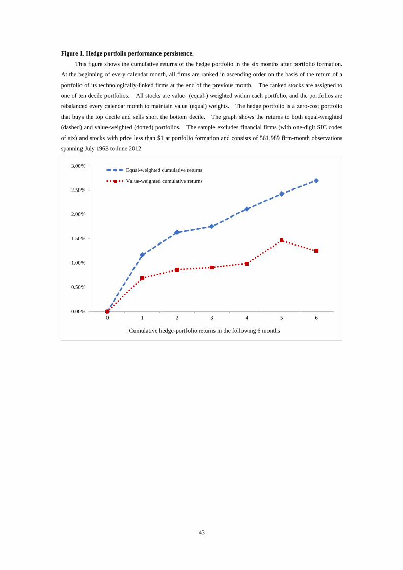
43
Figure 1. Hedge portfolio performance persistence.
This figure shows the cumulative returns of the hedge portfolio in the six months after portfolio formation.
At the beginning of every calendar month, all firms are ranked in ascending order on the basis of the return of a
portfolio of its technologically-linked firms at the end of the previous month. The ranked stocks are assigned to
one of ten decile portfolios. All stocks are value- (equal-) weighted within each portfolio, and the portfolios are
rebalanced every calendar month to maintain value (equal) weights. The hedge portfolio is a zero-cost portfolio
that buys the top decile and sells short the bottom decile. The graph shows the returns to both equal-weighted
(dashed) and value-weighted (dotted) portfolios. The sample excludes financial firms (with one-digit SIC codes
of six) and stocks with price less than $1 at portfolio formation and consists of 561,989 firm-month observations
spanning July 1963 to June 2012.
0.00%
0.50%
1.00%
1.50%
2.00%
2.50%
3.00%
0 1 2 3 4 5 6
Cumulative hedge-portfolio returns in the following 6 months
Equal-weighted cumulative returns
Value-weighted cumulative returns
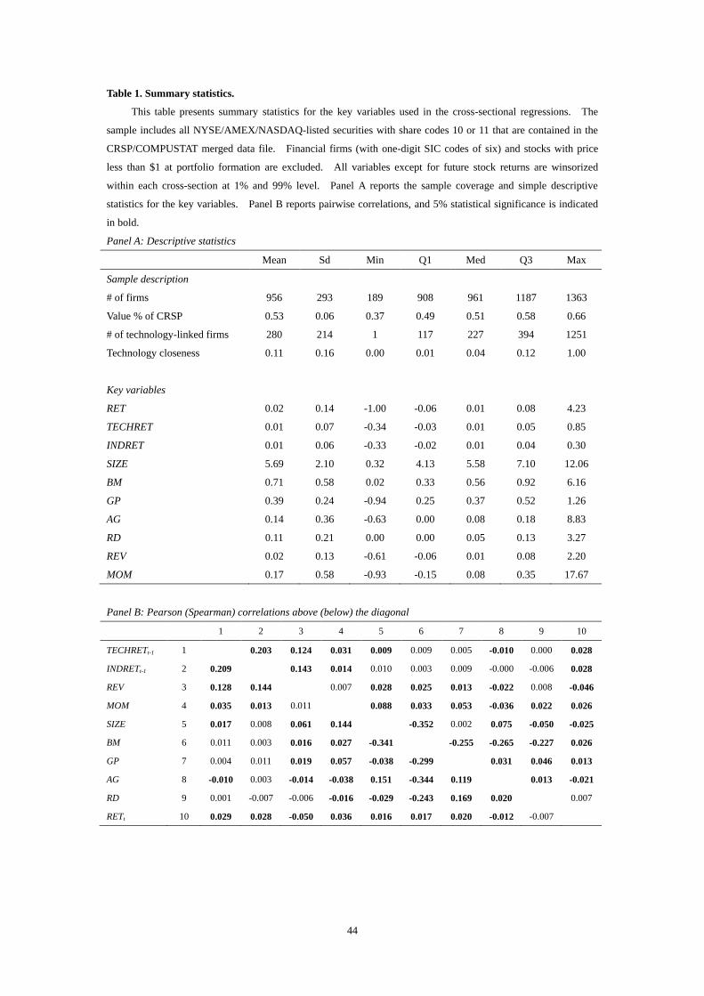
44
Table 1. Summary statistics.
This table presents summary statistics for the key variables used in the cross-sectional regressions. The
sample includes all NYSE/AMEX/NASDAQ-listed securities with share codes 10 or 11 that are contained in the
CRSP/COMPUSTAT merged data file. Financial firms (with one-digit SIC codes of six) and stocks with price
less than $1 at portfolio formation are excluded. All variables except for future stock returns are winsorized
within each cross-section at 1% and 99% level. Panel A reports the sample coverage and simple descriptive
statistics for the key variables. Panel B reports pairwise correlations, and 5% statistical significance is indicated
in bold.
Panel A: Descriptive statistics
Mean Sd Min Q1 Med Q3 Max
Sample description
# of firms 956 293 189 908 961 1187 1363
Value % of CRSP 0.53 0.06 0.37 0.49 0.51 0.58 0.66
# of technology-linked firms 280 214 1 117 227 394 1251
Technology closeness 0.11 0.16 0.00 0.01 0.04 0.12 1.00
Key variables
RET 0.02 0.14 -1.00 -0.06 0.01 0.08 4.23
TECHRET 0.01 0.07 -0.34 -0.03 0.01 0.05 0.85
INDRET 0.01 0.06 -0.33 -0.02 0.01 0.04 0.30
SIZE 5.69 2.10 0.32 4.13 5.58 7.10 12.06
BM 0.71 0.58 0.02 0.33 0.56 0.92 6.16
GP 0.39 0.24 -0.94 0.25 0.37 0.52 1.26
AG 0.14 0.36 -0.63 0.00 0.08 0.18 8.83
RD 0.11 0.21 0.00 0.00 0.05 0.13 3.27
REV 0.02 0.13 -0.61 -0.06 0.01 0.08 2.20
MOM 0.17 0.58 -0.93 -0.15 0.08 0.35 17.67
Panel B: Pearson (Spearman) correlations above (below) the diagonal
1 2 3 4 5 6 7 8 9 10
TECHRETt-1 1 0.203 0.124 0.031 0.009 0.009 0.005 -0.010 0.000 0.028
INDRETt-1 2 0.209 0.143 0.014 0.010 0.003 0.009 -0.000 -0.006 0.028
REV 3 0.128 0.144 0.007 0.028 0.025 0.013 -0.022 0.008 -0.046
MOM 4 0.035 0.013 0.011 0.088 0.033 0.053 -0.036 0.022 0.026
SIZE 5 0.017 0.008 0.061 0.144 -0.352 0.002 0.075 -0.050 -0.025
BM 6 0.011 0.003 0.016 0.027 -0.341 -0.255 -0.265 -0.227 0.026
GP 7 0.004 0.011 0.019 0.057 -0.038 -0.299 0.031 0.046 0.013
AG 8 -0.010 0.003 -0.014 -0.038 0.151 -0.344 0.119 0.013 -0.021
RD 9 0.001 -0.007 -0.006 -0.016 -0.029 -0.243 0.169 0.020 0.007
RETt 10 0.029 0.028 -0.050 0.036 0.016 0.017 0.020 -0.012 -0.007
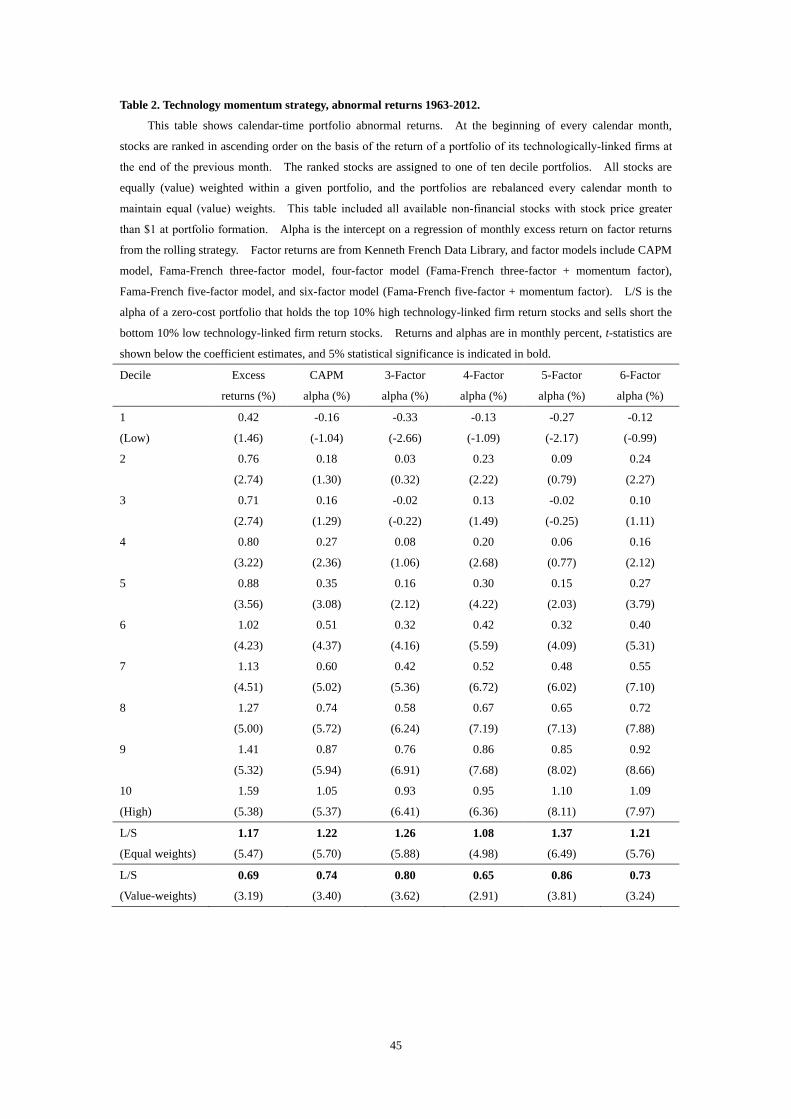
45
Table 2. Technology momentum strategy, abnormal returns 1963-2012.
This table shows calendar-time portfolio abnormal returns. At the beginning of every calendar month,
stocks are ranked in ascending order on the basis of the return of a portfolio of its technologically-linked firms at
the end of the previous month. The ranked stocks are assigned to one of ten decile portfolios. All stocks are
equally (value) weighted within a given portfolio, and the portfolios are rebalanced every calendar month to
maintain equal (value) weights. This table included all available non-financial stocks with stock price greater
than $1 at portfolio formation. Alpha is the intercept on a regression of monthly excess return on factor returns
from the rolling strategy. Factor returns are from Kenneth French Data Library, and factor models include CAPM
model, Fama-French three-factor model, four-factor model (Fama-French three-factor + momentum factor),
Fama-French five-factor model, and six-factor model (Fama-French five-factor + momentum factor). L/S is the
alpha of a zero-cost portfolio that holds the top 10% high technology-linked firm return stocks and sells short the
bottom 10% low technology-linked firm return stocks. Returns and alphas are in monthly percent, t-statistics are
shown below the coefficient estimates, and 5% statistical significance is indicated in bold.
Decile Excess
returns (%)
CAPM
alpha (%)
3-Factor
alpha (%)
4-Factor
alpha (%)
5-Factor
alpha (%)
6-Factor
alpha (%)
1 0.42 -0.16 -0.33 -0.13 -0.27 -0.12
(Low) (1.46) (-1.04) (-2.66) (-1.09) (-2.17) (-0.99)
2 0.76 0.18 0.03 0.23 0.09 0.24
(2.74) (1.30) (0.32) (2.22) (0.79) (2.27)
3 0.71 0.16 -0.02 0.13 -0.02 0.10
(2.74) (1.29) (-0.22) (1.49) (-0.25) (1.11)
4 0.80 0.27 0.08 0.20 0.06 0.16
(3.22) (2.36) (1.06) (2.68) (0.77) (2.12)
5 0.88 0.35 0.16 0.30 0.15 0.27
(3.56) (3.08) (2.12) (4.22) (2.03) (3.79)
6 1.02 0.51 0.32 0.42 0.32 0.40
(4.23) (4.37) (4.16) (5.59) (4.09) (5.31)
7 1.13 0.60 0.42 0.52 0.48 0.55
(4.51) (5.02) (5.36) (6.72) (6.02) (7.10)
8 1.27 0.74 0.58 0.67 0.65 0.72
(5.00) (5.72) (6.24) (7.19) (7.13) (7.88)
9 1.41 0.87 0.76 0.86 0.85 0.92
(5.32) (5.94) (6.91) (7.68) (8.02) (8.66)
10 1.59 1.05 0.93 0.95 1.10 1.09
(High) (5.38) (5.37) (6.41) (6.36) (8.11) (7.97)
L/S 1.17 1.22 1.26 1.08 1.37 1.21
(Equal weights) (5.47) (5.70) (5.88) (4.98) (6.49) (5.76)
L/S 0.69 0.74 0.80 0.65 0.86 0.73
(Value-weights) (3.19) (3.40) (3.62) (2.91) (3.81) (3.24)
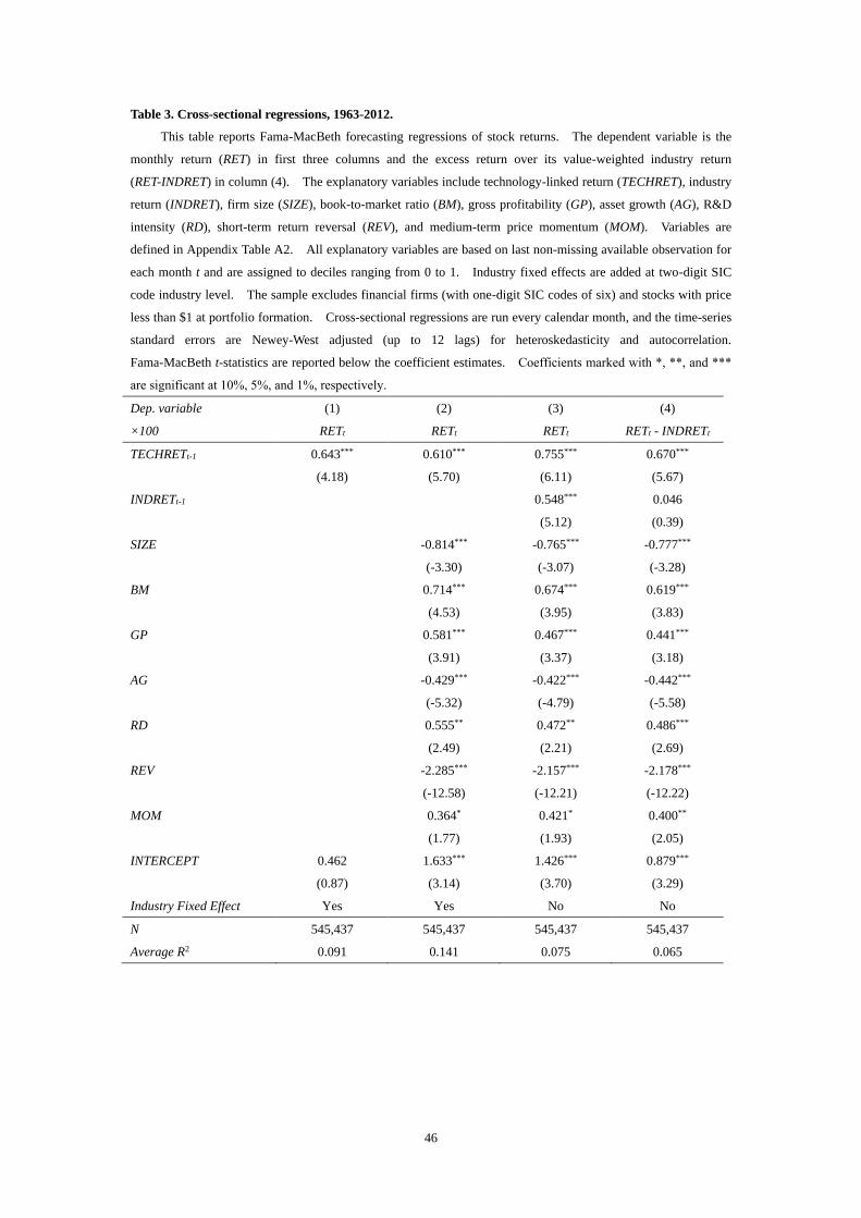
46
Table 3. Cross-sectional regressions, 1963-2012.
This table reports Fama-MacBeth forecasting regressions of stock returns. The dependent variable is the
monthly return (RET) in first three columns and the excess return over its value-weighted industry return
(RET-INDRET) in column (4). The explanatory variables include technology-linked return (TECHRET), industry
return (INDRET), firm size (SIZE), book-to-market ratio (BM), gross profitability (GP), asset growth (AG), R&D
intensity (RD), short-term return reversal (REV), and medium-term price momentum (MOM). Variables are
defined in Appendix Table A2. All explanatory variables are based on last non-missing available observation for
each month t and are assigned to deciles ranging from 0 to 1. Industry fixed effects are added at two-digit SIC
code industry level. The sample excludes financial firms (with one-digit SIC codes of six) and stocks with price
less than $1 at portfolio formation. Cross-sectional regressions are run every calendar month, and the time-series
standard errors are Newey-West adjusted (up to 12 lags) for heteroskedasticity and autocorrelation.
Fama-MacBeth t-statistics are reported below the coefficient estimates. Coefficients marked with *, **, and ***
are significant at 10%, 5%, and 1%, respectively.
Dep. variable (1) (2) (3) (4)
×100 RETt RETt RETt RETt - INDRETt
TECHRETt-1 0.643*** 0.610*** 0.755*** 0.670***
(4.18) (5.70) (6.11) (5.67)
INDRETt-1 0.548*** 0.046
(5.12) (0.39)
SIZE -0.814*** -0.765*** -0.777***
(-3.30) (-3.07) (-3.28)
BM 0.714*** 0.674*** 0.619***
(4.53) (3.95) (3.83)
GP 0.581*** 0.467*** 0.441***
(3.91) (3.37) (3.18)
AG -0.429*** -0.422*** -0.442***
(-5.32) (-4.79) (-5.58)
RD 0.555** 0.472** 0.486***
(2.49) (2.21) (2.69)
REV -2.285*** -2.157*** -2.178***
(-12.58) (-12.21) (-12.22)
MOM 0.364* 0.421* 0.400**
(1.77) (1.93) (2.05)
INTERCEPT 0.462 1.633*** 1.426*** 0.879***
(0.87) (3.14) (3.70) (3.29)
Industry Fixed Effect Yes Yes No No
N 545,437 545,437 545,437 545,437
Average R2 0.091 0.141 0.075 0.065
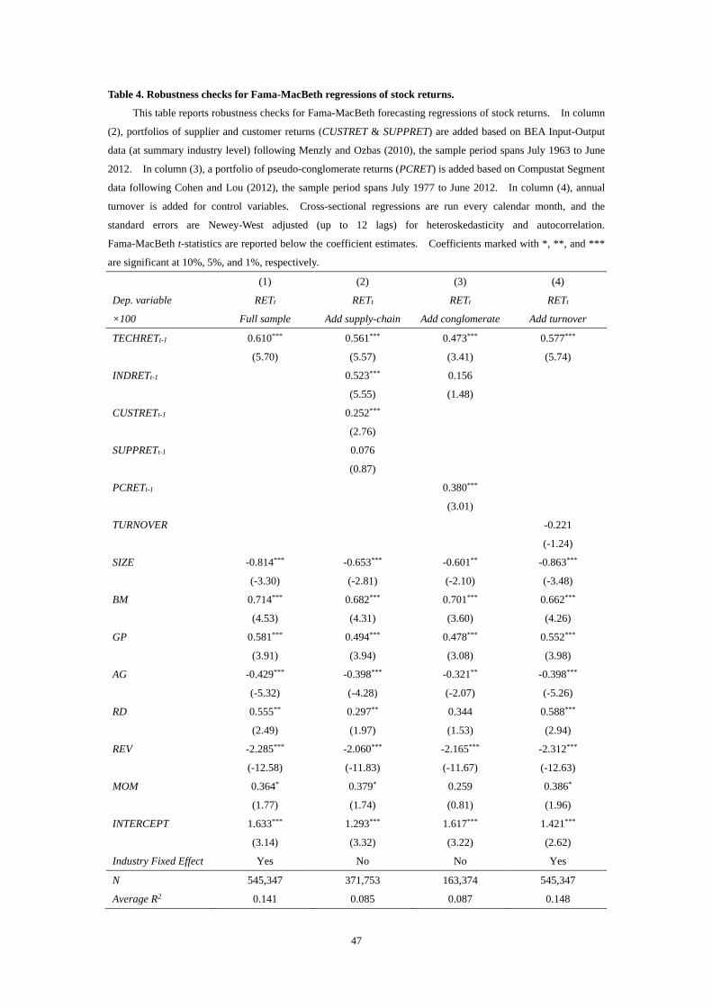
47
Table 4. Robustness checks for Fama-MacBeth regressions of stock returns.
This table reports robustness checks for Fama-MacBeth forecasting regressions of stock returns. In column
(2), portfolios of supplier and customer returns (CUSTRET & SUPPRET) are added based on BEA Input-Output
data (at summary industry level) following Menzly and Ozbas (2010), the sample period spans July 1963 to June
2012. In column (3), a portfolio of pseudo-conglomerate returns (PCRET) is added based on Compustat Segment
data following Cohen and Lou (2012), the sample period spans July 1977 to June 2012. In column (4), annual
turnover is added for control variables. Cross-sectional regressions are run every calendar month, and the
standard errors are Newey-West adjusted (up to 12 lags) for heteroskedasticity and autocorrelation.
Fama-MacBeth t-statistics are reported below the coefficient estimates. Coefficients marked with *, **, and ***
are significant at 10%, 5%, and 1%, respectively.
(1) (2) (3) (4)
Dep. variable RETt RETt RETt RETt
×100 Full sample Add supply-chain Add conglomerate Add turnover
TECHRETt-1 0.610*** 0.561*** 0.473*** 0.577***
(5.70) (5.57) (3.41) (5.74)
INDRETt-1 0.523*** 0.156
(5.55) (1.48)
CUSTRETt-1 0.252***
(2.76)
SUPPRETt-1 0.076
(0.87)
PCRETt-1 0.380***
(3.01)
TURNOVER -0.221
(-1.24)
SIZE -0.814*** -0.653*** -0.601** -0.863***
(-3.30) (-2.81) (-2.10) (-3.48)
BM 0.714*** 0.682*** 0.701*** 0.662***
(4.53) (4.31) (3.60) (4.26)
GP 0.581*** 0.494*** 0.478*** 0.552***
(3.91) (3.94) (3.08) (3.98)
AG -0.429*** -0.398*** -0.321** -0.398***
(-5.32) (-4.28) (-2.07) (-5.26)
RD 0.555** 0.297** 0.344 0.588***
(2.49) (1.97) (1.53) (2.94)
REV -2.285*** -2.060*** -2.165*** -2.312***
(-12.58) (-11.83) (-11.67) (-12.63)
MOM 0.364* 0.379* 0.259 0.386*
(1.77) (1.74) (0.81) (1.96)
INTERCEPT 1.633*** 1.293*** 1.617*** 1.421***
(3.14) (3.32) (3.22) (2.62)
Industry Fixed Effect Yes No No Yes
N 545,347 371,753 163,374 545,347
Average R2 0.141 0.085 0.087 0.148
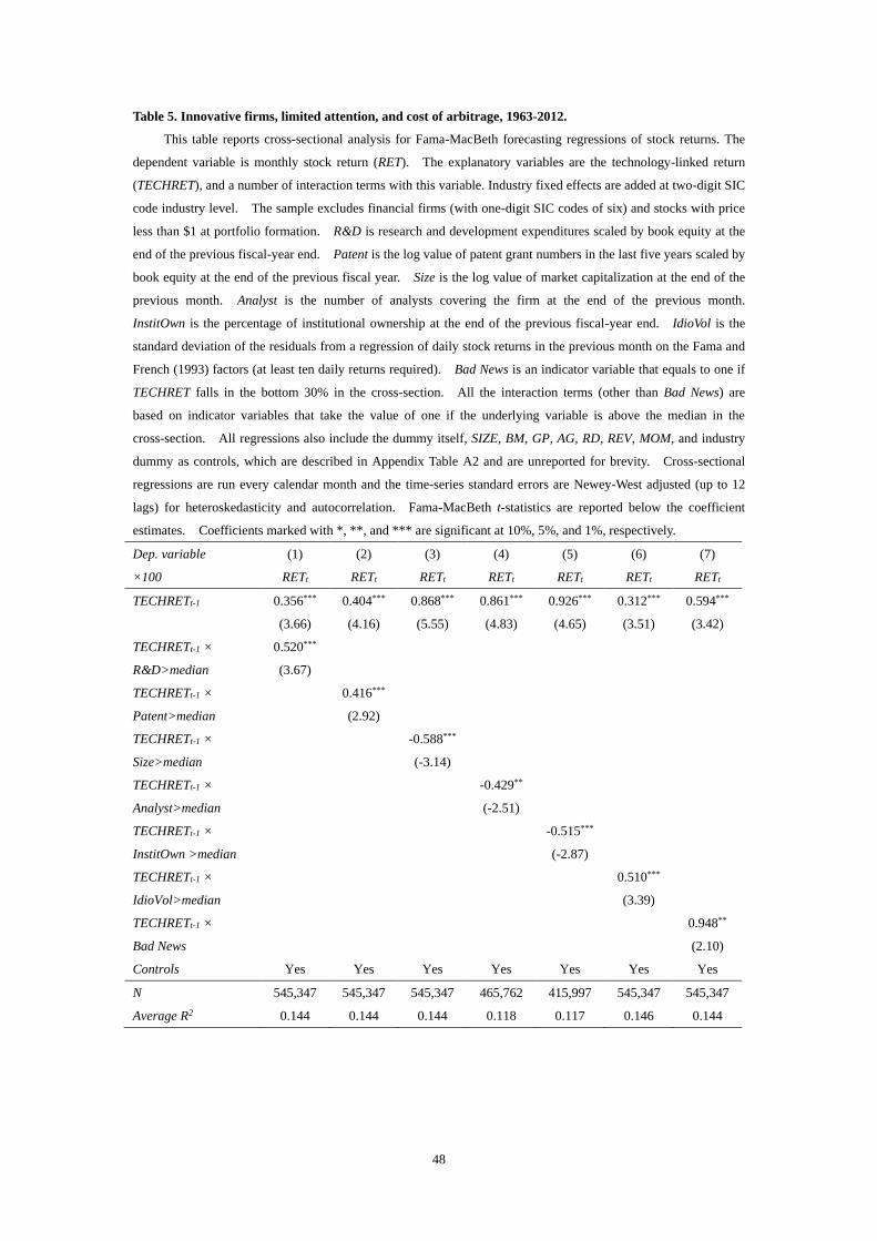
48
Table 5. Innovative firms, limited attention, and cost of arbitrage, 1963-2012.
This table reports cross-sectional analysis for Fama-MacBeth forecasting regressions of stock returns. The
dependent variable is monthly stock return (RET). The explanatory variables are the technology-linked return
(TECHRET), and a number of interaction terms with this variable. Industry fixed effects are added at two-digit SIC
code industry level. The sample excludes financial firms (with one-digit SIC codes of six) and stocks with price
less than $1 at portfolio formation. R&D is research and development expenditures scaled by book equity at the
end of the previous fiscal-year end. Patent is the log value of patent grant numbers in the last five years scaled by
book equity at the end of the previous fiscal year. Size is the log value of market capitalization at the end of the
previous month. Analyst is the number of analysts covering the firm at the end of the previous month.
InstitOwn is the percentage of institutional ownership at the end of the previous fiscal-year end. IdioVol is the
standard deviation of the residuals from a regression of daily stock returns in the previous month on the Fama and
French (1993) factors (at least ten daily returns required). Bad News is an indicator variable that equals to one if
TECHRET falls in the bottom 30% in the cross-section. All the interaction terms (other than Bad News) are
based on indicator variables that take the value of one if the underlying variable is above the median in the
cross-section. All regressions also include the dummy itself, SIZE, BM, GP, AG, RD, REV, MOM, and industry
dummy as controls, which are described in Appendix Table A2 and are unreported for brevity. Cross-sectional
regressions are run every calendar month and the time-series standard errors are Newey-West adjusted (up to 12
lags) for heteroskedasticity and autocorrelation. Fama-MacBeth t-statistics are reported below the coefficient
estimates. Coefficients marked with *, **, and *** are significant at 10%, 5%, and 1%, respectively.
Dep. variable (1) (2) (3) (4) (5) (6) (7)
×100 RETt RETt RETt RETt RETt RETt RETt
TECHRETt-1 0.356*** 0.404*** 0.868*** 0.861*** 0.926*** 0.312*** 0.594***
(3.66) (4.16) (5.55) (4.83) (4.65) (3.51) (3.42)
TECHRETt-1 × 0.520***
R&D>median (3.67)
TECHRETt-1 × 0.416***
Patent>median (2.92)
TECHRETt-1 × -0.588***
Size>median (-3.14)
TECHRETt-1 × -0.429**
Analyst>median (-2.51)
TECHRETt-1 × -0.515***
InstitOwn >median (-2.87)
TECHRETt-1 × 0.510***
IdioVol>median (3.39)
TECHRETt-1 × 0.948**
Bad News (2.10)
Controls Yes Yes Yes Yes Yes Yes Yes
N 545,347 545,347 545,347 465,762 415,997 545,347 545,347
Average R2 0.144 0.144 0.144 0.118 0.117 0.146 0.144
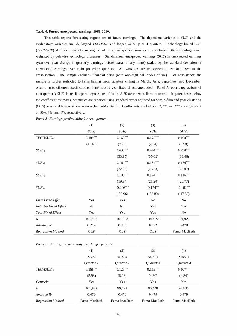
49
Table 6. Future unexpected earnings, 1966-2010.
This table reports forecasting regressions of future earnings. The dependent variable is SUE, and the
explanatory variables include lagged TECHSUE and lagged SUE up to 4 quarters. Technology-linked SUE
(TECHSUE) of a focal firm is the average standardized unexpected earnings of other firms in the technology space
weighted by pairwise technology closeness. Standardized unexpected earnings (SUE) is unexpected earnings
(year-over-year change in quarterly earnings before extraordinary items) scaled by the standard deviation of
unexpected earnings over eight preceding quarters. All variables are winsorized at 1% and 99% in the
cross-section. The sample excludes financial firms (with one-digit SIC codes of six). For consistency, the
sample is further restricted to firms having fiscal quarters ending in March, June, September, and December.
According to different specifications, firm/industry/year fixed effects are added. Panel A reports regressions of
next quarter’s SUE; Panel B reports regressions of future SUE over next 4 fiscal quarters. In parentheses below
the coefficient estimates, t-statistics are reported using standard errors adjusted for within-firm and year clustering
(OLS) or up to 4 lags serial correlation (Fama-MacBeth). Coefficients marked with *, **, and *** are significant
at 10%, 5%, and 1%, respectively.
Panel A: Earnings predictability for next quarter
(1) (2) (3) (4)
SUEt SUEt SUEt SUEt
TECHSUEt-1 0.489*** 0.166*** 0.175*** 0.168***
(11.69) (7.73) (7.94) (5.98)
SUEt-1 0.438*** 0.474*** 0.490***
(33.95) (35.02) (38.46)
SUEt-2 0.164*** 0.184*** 0.176***
(22.93) (23.53) (25.07)
SUEt-3 0.106*** 0.124*** 0.116***
(19.94) (21.20) (20.77)
SUEt-4 -0.206*** -0.174*** -0.162***
(-30.96) (-23.80) (-17.80)
Firm Fixed Effect Yes Yes No No
Industry Fixed Effect No No Yes Yes
Year Fixed Effect Yes Yes Yes No
N 101,922 101,922 101,922 101,922
Adj/Avg. R2 0.219 0.458 0.432 0.479
Regression Method OLS OLS OLS Fama-MacBeth
Panel B: Earnings predictability over longer periods
(1) (2) (3) (4)
SUEt SUEt+1 SUEt+2 SUEt+3
Quarter 1 Quarter 2 Quarter 3 Quarter 4
TECHSUEt-1 0.168*** 0.128*** 0.113*** 0.107***
(5.98) (5.18) (4.60) (4.84)
Controls Yes Yes Yes Yes
N 101,922 99,179 96,448 93,835
Average R2 0.479 0.479 0.479 0.479
Regression Method Fama-MacBeth Fama-MacBeth Fama-MacBeth Fama-MacBeth
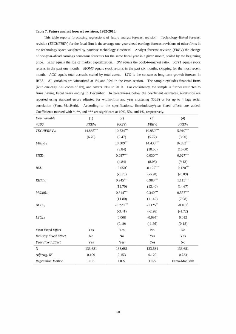
50
Table 7. Future analyst forecast revisions, 1982-2010.
This table reports forecasting regressions of future analyst forecast revision. Technology-linked forecast
revision (TECHFREV) for the focal firm is the average one-year-ahead earnings forecast revisions of other firms in
the technology space weighted by pairwise technology closeness. Analyst forecast revision (FREV) the change
of one-year-ahead earnings consensus forecasts for the same fiscal year in a given month, scaled by the beginning
price. SIZE equals the log of market capitalization. BM equals the book-to-market ratio. RET1 equals stock
returns in the past one month. MOM6 equals stock returns in the past six months, skipping for the most recent
month. ACC equals total accruals scaled by total assets. LTG is the consensus long-term growth forecast in
IBES. All variables are winsorized at 1% and 99% in the cross-section. The sample excludes financial firms
(with one-digit SIC codes of six), and covers 1982 to 2010. For consistency, the sample is further restricted to
firms having fiscal years ending in December. In parentheses below the coefficient estimates, t-statistics are
reported using standard errors adjusted for within-firm and year clustering (OLS) or for up to 4 lags serial
correlation (Fama-MacBeth). According to the specifications, firm/industry/year fixed effects are added.
Coefficients marked with *, **, and *** are significant at 10%, 5%, and 1%, respectively.
Dep. variable (1) (2) (3) (4)
×100 FREVt FREVt FREVt FREVt
TECHFREVt-1 14.885*** 10.534*** 10.950*** 5.919***
(6.76) (5.47) (5.72) (3.90)
FREVt-1 10.309*** 14.430*** 16.892***
(8.84) (10.50) (10.60)
SIZEt-1 0.087*** 0.030*** 0.027***
(4.84) (8.03) (9.13)
BMt-1 -0.050* -0.125*** -0.120***
(-1.78) (-6.28) (-5.09)
RET1t-1 0.945*** 0.983*** 1.115***
(12.70) (12.40) (14.67)
MOM6t-1 0.314*** 0.340*** 0.557***
(11.80) (11.42) (7.98)
ACCt-1 -0.220*** -0.125** -0.101*
(-3.41) (-2.26) (-1.72)
LTGt-1 0.008 -0.095* 0.012
(0.10) (-1.86) (0.18)
Firm Fixed Effect Yes Yes No No
Industry Fixed Effect No No Yes Yes
Year Fixed Effect Yes Yes Yes No
N 133,681 133,681 133,681 133,681
Adj/Avg. R2 0.109 0.153 0.120 0.233
Regression Method OLS OLS OLS Fama-MacBeth
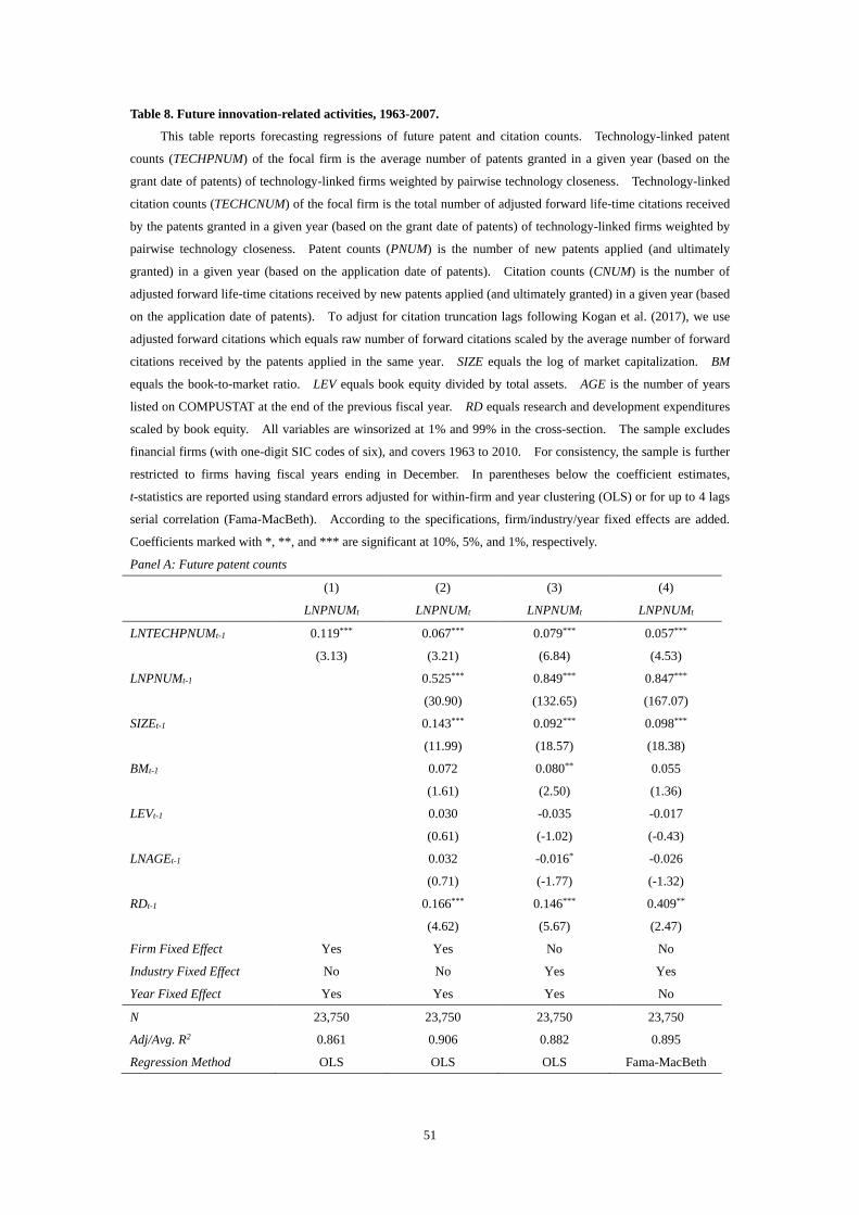
51
Table 8. Future innovation-related activities, 1963-2007.
This table reports forecasting regressions of future patent and citation counts. Technology-linked patent
counts (TECHPNUM) of the focal firm is the average number of patents granted in a given year (based on the
grant date of patents) of technology-linked firms weighted by pairwise technology closeness. Technology-linked
citation counts (TECHCNUM) of the focal firm is the total number of adjusted forward life-time citations received
by the patents granted in a given year (based on the grant date of patents) of technology-linked firms weighted by
pairwise technology closeness. Patent counts (PNUM) is the number of new patents applied (and ultimately
granted) in a given year (based on the application date of patents). Citation counts (CNUM) is the number of
adjusted forward life-time citations received by new patents applied (and ultimately granted) in a given year (based
on the application date of patents). To adjust for citation truncation lags following Kogan et al. (2017), we use
adjusted forward citations which equals raw number of forward citations scaled by the average number of forward
citations received by the patents applied in the same year. SIZE equals the log of market capitalization. BM
equals the book-to-market ratio. LEV equals book equity divided by total assets. AGE is the number of years
listed on COMPUSTAT at the end of the previous fiscal year. RD equals research and development expenditures
scaled by book equity. All variables are winsorized at 1% and 99% in the cross-section. The sample excludes
financial firms (with one-digit SIC codes of six), and covers 1963 to 2010. For consistency, the sample is further
restricted to firms having fiscal years ending in December. In parentheses below the coefficient estimates,
t-statistics are reported using standard errors adjusted for within-firm and year clustering (OLS) or for up to 4 lags
serial correlation (Fama-MacBeth). According to the specifications, firm/industry/year fixed effects are added.
Coefficients marked with *, **, and *** are significant at 10%, 5%, and 1%, respectively.
Panel A: Future patent counts
(1) (2) (3) (4)
LNPNUMt LNPNUMt LNPNUMt LNPNUMt
LNTECHPNUMt-1 0.119*** 0.067*** 0.079*** 0.057***
(3.13) (3.21) (6.84) (4.53)
LNPNUMt-1 0.525*** 0.849*** 0.847***
(30.90) (132.65) (167.07)
SIZEt-1 0.143*** 0.092*** 0.098***
(11.99) (18.57) (18.38)
BMt-1 0.072 0.080** 0.055
(1.61) (2.50) (1.36)
LEVt-1 0.030 -0.035 -0.017
(0.61) (-1.02) (-0.43)
LNAGEt-1 0.032 -0.016* -0.026
(0.71) (-1.77) (-1.32)
RDt-1 0.166*** 0.146*** 0.409**
(4.62) (5.67) (2.47)
Firm Fixed Effect Yes Yes No No
Industry Fixed Effect No No Yes Yes
Year Fixed Effect Yes Yes Yes No
N 23,750 23,750 23,750 23,750
Adj/Avg. R2 0.861 0.906 0.882 0.895
Regression Method OLS OLS OLS Fama-MacBeth
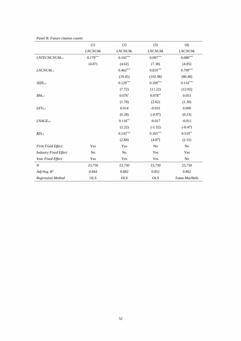
52
Panel B: Future citation counts
(1) (2) (3) (4)
LNCNUMt LNCNUMt LNCNUMt LNCNUMt
LNTECHCNUMt-1 0.179*** 0.102*** 0.097*** 0.080***
(4.87) (4.62) (7.38) (4.85)
LNCNUMt-1 0.462*** 0.810*** 0.799***
(19.45) (102.98) (86.48)
SIZEt-1 0.129*** 0.100*** 0.116***
(7.72) (11.22) (12.02)
BMt-1 0.076* 0.078** 0.053
(1.70) (2.62) (1.30)
LEVt-1 0.014 -0.031 0.009
(0.28) (-0.97) (0.23)
LNAGEt-1 0.116** -0.017 -0.011
(2.22) (-1.52) (-0.47)
RDt-1 0.143*** 0.165*** 0.519**
(2.84) (4.87) (2.31)
Firm Fixed Effect Yes Yes No No
Industry Fixed Effect No No Yes Yes
Year Fixed Effect Yes Yes Yes No
N 23,750 23,750 23,750 23,750
Adj/Avg. R2 0.844 0.882 0.851 0.862
Regression Method OLS OLS OLS Fama-MacBeth
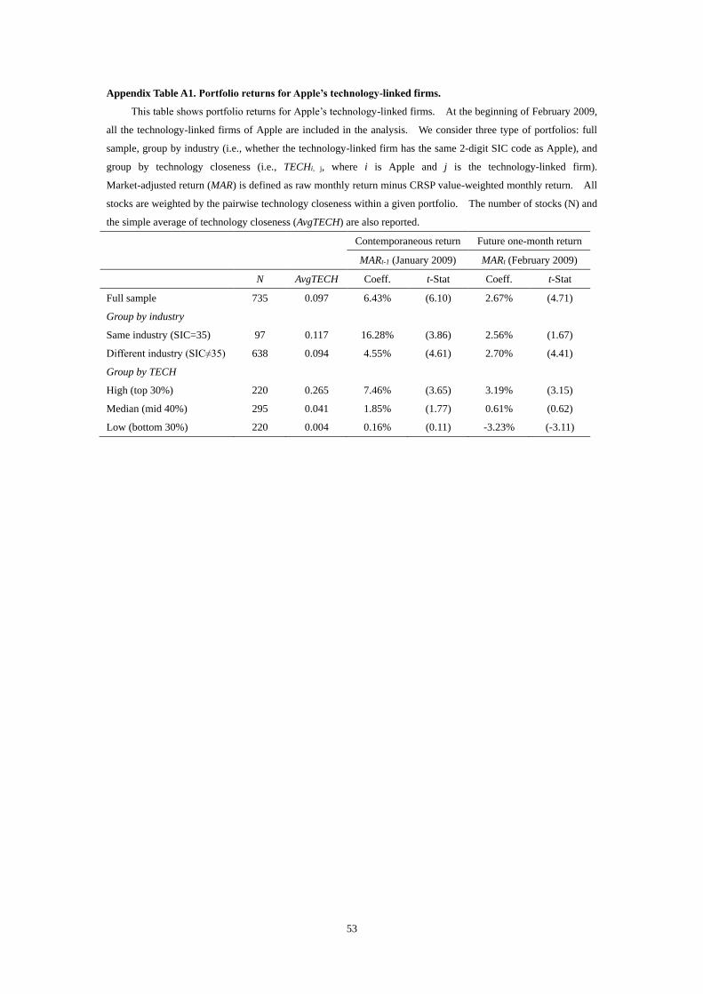
53
Appendix Table A1. Portfolio returns for Apple’s technology-linked firms.
This table shows portfolio returns for Apple’s technology-linked firms. At the beginning of February 2009,
all the technology-linked firms of Apple are included in the analysis. We consider three type of portfolios: full
sample, group by industry (i.e., whether the technology-linked firm has the same 2-digit SIC code as Apple), and
group by technology closeness (i.e., TECHi, j, where i is Apple and j is the technology-linked firm).
Market-adjusted return (MAR) is defined as raw monthly return minus CRSP value-weighted monthly return. All
stocks are weighted by the pairwise technology closeness within a given portfolio. The number of stocks (N) and
the simple average of technology closeness (AvgTECH) are also reported.
Contemporaneous return Future one-month return
MARt-1 (January 2009) MARt (February 2009)
N AvgTECH Coeff. t-Stat Coeff. t-Stat
Full sample 735 0.097 6.43% (6.10) 2.67% (4.71)
Group by industry
Same industry (SIC=35) 97 0.117 16.28% (3.86) 2.56% (1.67)
Different industry (SIC≠35) 638 0.094 4.55% (4.61) 2.70% (4.41)
Group by TECH
High (top 30%) 220 0.265 7.46% (3.65) 3.19% (3.15)
Median (mid 40%) 295 0.041 1.85% (1.77) 0.61% (0.62)
Low (bottom 30%) 220 0.004 0.16% (0.11) -3.23% (-3.11)
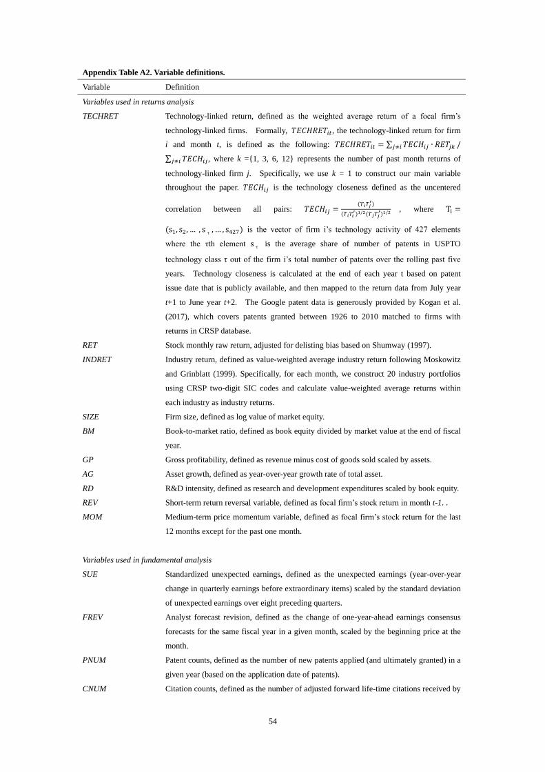
54
Appendix Table A2. Variable definitions.
Variable Definition
Variables used in returns analysis
TECHRET
Technology-linked return, defined as the weighted average return of a focal firm’s
technology-linked firms. Formally, 𝑇𝐸𝐶𝐻𝑅𝐸𝑇𝑖𝑡, the technology-linked return for firm
i and month t, is defined as the following: 𝑇𝐸𝐶𝐻𝑅𝐸𝑇𝑖𝑡 = ∑ 𝑇𝐸𝐶𝐻𝑖𝑗 ∙ 𝑅𝐸𝑇𝑗𝑘𝑗≠𝑖 /
∑ 𝑇𝐸𝐶𝐻𝑖𝑗𝑗≠𝑖 , where k ={1, 3, 6, 12} represents the number of past month returns of
technology-linked firm j. Specifically, we use k = 1 to construct our main variable
throughout the paper. 𝑇𝐸𝐶𝐻𝑖𝑗 is the technology closeness defined as the uncentered
correlation between all pairs: 𝑇𝐸𝐶𝐻𝑖𝑗 =(𝑇𝑖𝑇𝑗
′)
(𝑇𝑖𝑇𝑖′)1/2(𝑇𝑗𝑇𝑗
′)1/2, where Ti =
(s1, s2, … , sτ, … , s427) is the vector of firm i’s technology activity of 427 elements
where the τth element sτ is the average share of number of patents in USPTO
technology class τ out of the firm i’s total number of patents over the rolling past five
years. Technology closeness is calculated at the end of each year t based on patent
issue date that is publicly available, and then mapped to the return data from July year
t+1 to June year t+2. The Google patent data is generously provided by Kogan et al.
(2017), which covers patents granted between 1926 to 2010 matched to firms with
returns in CRSP database.
RET Stock monthly raw return, adjusted for delisting bias based on Shumway (1997).
INDRET Industry return, defined as value-weighted average industry return following Moskowitz
and Grinblatt (1999). Specifically, for each month, we construct 20 industry portfolios
using CRSP two-digit SIC codes and calculate value-weighted average returns within
each industry as industry returns.
SIZE Firm size, defined as log value of market equity.
BM Book-to-market ratio, defined as book equity divided by market value at the end of fiscal
year.
GP Gross profitability, defined as revenue minus cost of goods sold scaled by assets.
AG Asset growth, defined as year-over-year growth rate of total asset.
RD R&D intensity, defined as research and development expenditures scaled by book equity.
REV Short-term return reversal variable, defined as focal firm’s stock return in month t-1. .
MOM Medium-term price momentum variable, defined as focal firm’s stock return for the last
12 months except for the past one month.
Variables used in fundamental analysis
SUE Standardized unexpected earnings, defined as the unexpected earnings (year-over-year
change in quarterly earnings before extraordinary items) scaled by the standard deviation
of unexpected earnings over eight preceding quarters.
FREV Analyst forecast revision, defined as the change of one-year-ahead earnings consensus
forecasts for the same fiscal year in a given month, scaled by the beginning price at the
month.
PNUM Patent counts, defined as the number of new patents applied (and ultimately granted) in a
given year (based on the application date of patents).
CNUM Citation counts, defined as the number of adjusted forward life-time citations received by

55
new patents applied (and ultimately granted) in a given year (based on the application
date of patents). To adjust for citation truncation lags following Kogan et al. (2017), we
use adjusted forward citations which equals raw number of forward citations scaled by
the average number of forward citations received by the patents applied in the same year.
TECHSUE Technology-linked SUE, defined as the average of standardized unexpected earnings
weighted by pairwise technology closeness. For consistency, the sample is restricted to
firms having fiscal quarters ending in March, June, September, and December.
TECHFREV Technology-linked forecast revision, defined as the average of one-year-ahead earnings
forecast revisions in a given month weighted by pairwise technology closeness. For
consistency, the sample is restricted to firms having fiscal years ending in December.
TECHPNUM Technology-linked patent counts, defined as the average number of patents granted in a
given year (based on the grant date of patents) of technology-linked firms weighted by
pairwise technology closeness. For consistency, the sample is restricted to firms having
fiscal years ending in December.
TECHCNUM Technology-linked citation counts, defined as the total number of adjusted forward
life-time citations received by new patents granted in a given year (based on the grant
date of patents) of technology-linked firms weighted by pairwise technology closeness.
For consistency, the sample is restricted to firms having fiscal years ending in December.
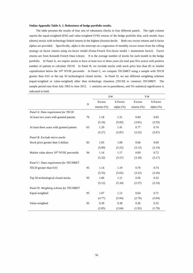
56
Online Appendix Table A. 1. Robustness of hedge portfolio results.
The table presents the results of four sets of robustness checks in four different panels. The right column
reports the equal-weighted (EW) and value-weighted (VW) returns of the hedge portfolio that, each month, buys
(shorts) stocks with technology-linked returns in the highest (lowest) decile. Both raw excess returns and 6-factor
alphas are provided. Specifically, alpha is the intercept on a regression of monthly excess return from the rolling
strategy on factor returns using six-factor model (Fama-French five-factor model + momentum factor). Factor
returns are from Kenneth French Data Library. N is the average number of stocks for each month in the hedge
portfolio. In Panel A, we require stocks to have at least two or three years (in total past five years) with positive
number of patents to calculate TECH. In Panel B, we exclude stocks with stock price less than $5 or market
capitalization below the 10th NYSE percentile. In Panel C, we compute TECHRET using a sample with TECH
greater than 0.01 or the top 50 technological closed stocks. In Panel D, we use different weighting schemes
(equal-weighted or value-weighted) other than technology closeness (TECH) to construct TECHRET. The
sample period runs from July 1963 to June 2012. t -statistics are in parentheses, and 5% statistical significance is
indicated in bold.
EW VW
N Excess
returns (%)
6-Factor
alpha (%)
Excess
returns (%)
6-Factor
alpha (%)
Panel A: Data requirement for TECH
At least two years with granted patents 76 1.18 1.31 0.84 0.83
(5.16) (5.83) (3.81) (3.55)
At least three years with granted patents 63 1.29 1.41 0.77 0.74
(5.27) (5.87) (3.32) (3.07)
Panel B: Exclude micro stocks
Stock price greater than 5 dollars 83 1.05 1.08 0.66 0.69
(5.00) (5.22) (3.12) (3.14)
Market value above 10th NYSE percentile 94 1.14 1.17 0.69 0.72
(5.32) (5.57) (3.18) (3.17)
Panel C: Data requirement for TECHRET
TECH greater than 0.01 95 1.14 1.19 0.70 0.74
(5.35) (5.65) (3.22) (3.26)
Top 50 technological closed stocks 95 1.06 1.11 0.56 0.53
(5.12) (5.34) (2.57) (2.33)
Panel D: Weighting scheme for TECHRET
Equal-weighted 95 1.07 1.12 0.64 0.71
(4.77) (5.04) (2.76) (3.04)
Value-weighted 95 0.39 0.38 0.36 0.35
(2.85) (2.64) (1.92) (1.70)
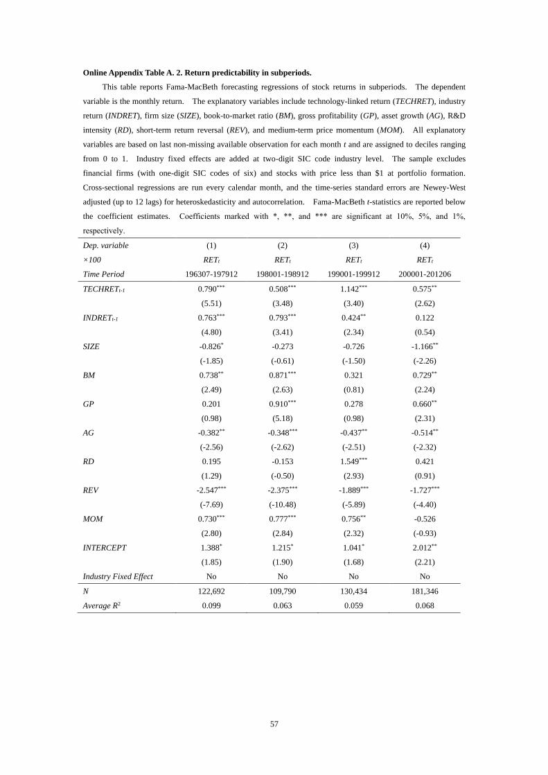
57
Online Appendix Table A. 2. Return predictability in subperiods.
This table reports Fama-MacBeth forecasting regressions of stock returns in subperiods. The dependent
variable is the monthly return. The explanatory variables include technology-linked return (TECHRET), industry
return (INDRET), firm size (SIZE), book-to-market ratio (BM), gross profitability (GP), asset growth (AG), R&D
intensity (RD), short-term return reversal (REV), and medium-term price momentum (MOM). All explanatory
variables are based on last non-missing available observation for each month t and are assigned to deciles ranging
from 0 to 1. Industry fixed effects are added at two-digit SIC code industry level. The sample excludes
financial firms (with one-digit SIC codes of six) and stocks with price less than $1 at portfolio formation.
Cross-sectional regressions are run every calendar month, and the time-series standard errors are Newey-West
adjusted (up to 12 lags) for heteroskedasticity and autocorrelation. Fama-MacBeth t-statistics are reported below
the coefficient estimates. Coefficients marked with *, **, and *** are significant at 10%, 5%, and 1%,
respectively.
Dep. variable (1) (2) (3) (4)
×100 RETt RETt RETt RETt
Time Period 196307-197912 198001-198912 199001-199912 200001-201206
TECHRETt-1 0.790*** 0.508*** 1.142*** 0.575**
(5.51) (3.48) (3.40) (2.62)
INDRETt-1 0.763*** 0.793*** 0.424** 0.122
(4.80) (3.41) (2.34) (0.54)
SIZE -0.826* -0.273 -0.726 -1.166**
(-1.85) (-0.61) (-1.50) (-2.26)
BM 0.738** 0.871*** 0.321 0.729**
(2.49) (2.63) (0.81) (2.24)
GP 0.201 0.910*** 0.278 0.660**
(0.98) (5.18) (0.98) (2.31)
AG -0.382** -0.348*** -0.437** -0.514**
(-2.56) (-2.62) (-2.51) (-2.32)
RD 0.195 -0.153 1.549*** 0.421
(1.29) (-0.50) (2.93) (0.91)
REV -2.547*** -2.375*** -1.889*** -1.727***
(-7.69) (-10.48) (-5.89) (-4.40)
MOM 0.730*** 0.777*** 0.756** -0.526
(2.80) (2.84) (2.32) (-0.93)
INTERCEPT 1.388* 1.215* 1.041* 2.012**
(1.85) (1.90) (1.68) (2.21)
Industry Fixed Effect No No No No
N 122,692 109,790 130,434 181,346
Average R2 0.099 0.063 0.059 0.068
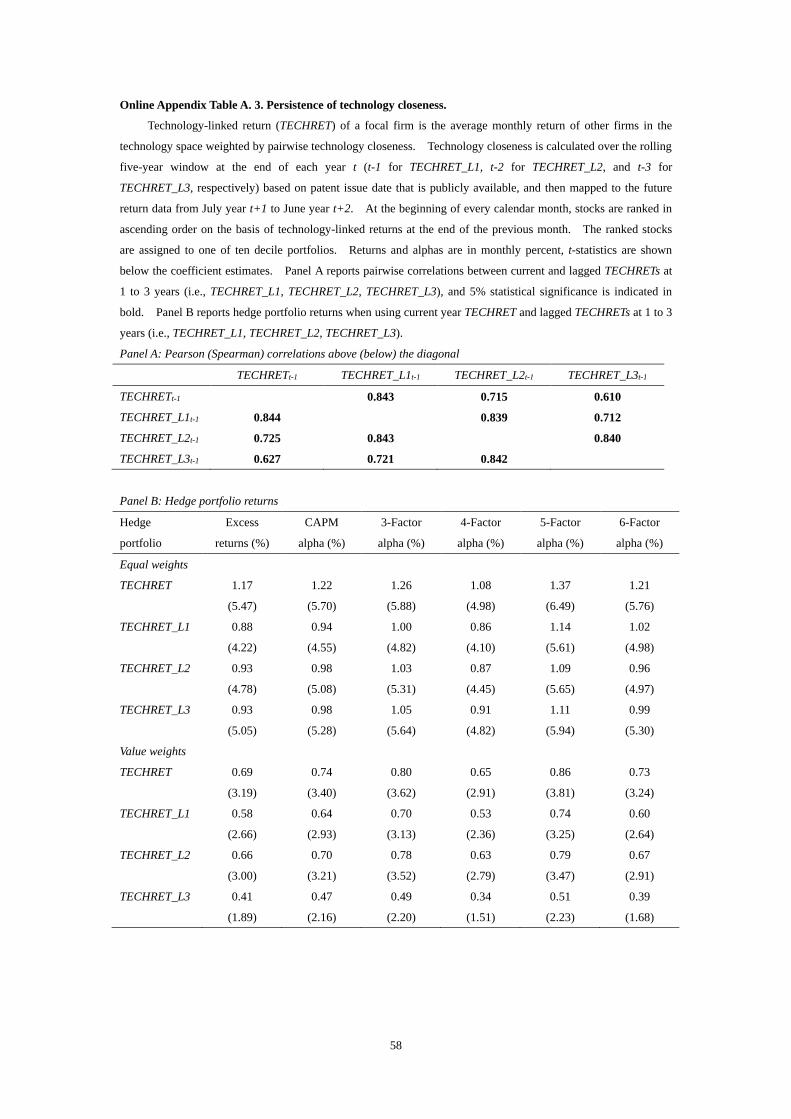
58
Online Appendix Table A. 3. Persistence of technology closeness.
Technology-linked return (TECHRET) of a focal firm is the average monthly return of other firms in the
technology space weighted by pairwise technology closeness. Technology closeness is calculated over the rolling
five-year window at the end of each year t (t-1 for TECHRET_L1, t-2 for TECHRET_L2, and t-3 for
TECHRET_L3, respectively) based on patent issue date that is publicly available, and then mapped to the future
return data from July year t+1 to June year t+2. At the beginning of every calendar month, stocks are ranked in
ascending order on the basis of technology-linked returns at the end of the previous month. The ranked stocks
are assigned to one of ten decile portfolios. Returns and alphas are in monthly percent, t-statistics are shown
below the coefficient estimates. Panel A reports pairwise correlations between current and lagged TECHRETs at
1 to 3 years (i.e., TECHRET_L1, TECHRET_L2, TECHRET_L3), and 5% statistical significance is indicated in
bold. Panel B reports hedge portfolio returns when using current year TECHRET and lagged TECHRETs at 1 to 3
years (i.e., TECHRET_L1, TECHRET_L2, TECHRET_L3).
Panel A: Pearson (Spearman) correlations above (below) the diagonal
TECHRETt-1 TECHRET_L1t-1 TECHRET_L2t-1 TECHRET_L3t-1
TECHRETt-1 0.843 0.715 0.610
TECHRET_L1t-1 0.844 0.839 0.712
TECHRET_L2t-1 0.725 0.843 0.840
TECHRET_L3t-1 0.627 0.721 0.842
Panel B: Hedge portfolio returns
Hedge
portfolio
Excess
returns (%)
CAPM
alpha (%)
3-Factor
alpha (%)
4-Factor
alpha (%)
5-Factor
alpha (%)
6-Factor
alpha (%)
Equal weights
TECHRET 1.17 1.22 1.26 1.08 1.37 1.21
(5.47) (5.70) (5.88) (4.98) (6.49) (5.76)
TECHRET_L1 0.88 0.94 1.00 0.86 1.14 1.02
(4.22) (4.55) (4.82) (4.10) (5.61) (4.98)
TECHRET_L2 0.93 0.98 1.03 0.87 1.09 0.96
(4.78) (5.08) (5.31) (4.45) (5.65) (4.97)
TECHRET_L3 0.93 0.98 1.05 0.91 1.11 0.99
(5.05) (5.28) (5.64) (4.82) (5.94) (5.30)
Value weights
TECHRET 0.69 0.74 0.80 0.65 0.86 0.73
(3.19) (3.40) (3.62) (2.91) (3.81) (3.24)
TECHRET_L1 0.58 0.64 0.70 0.53 0.74 0.60
(2.66) (2.93) (3.13) (2.36) (3.25) (2.64)
TECHRET_L2 0.66 0.70 0.78 0.63 0.79 0.67
(3.00) (3.21) (3.52) (2.79) (3.47) (2.91)
TECHRET_L3 0.41 0.47 0.49 0.34 0.51 0.39
(1.89) (2.16) (2.20) (1.51) (2.23) (1.68)
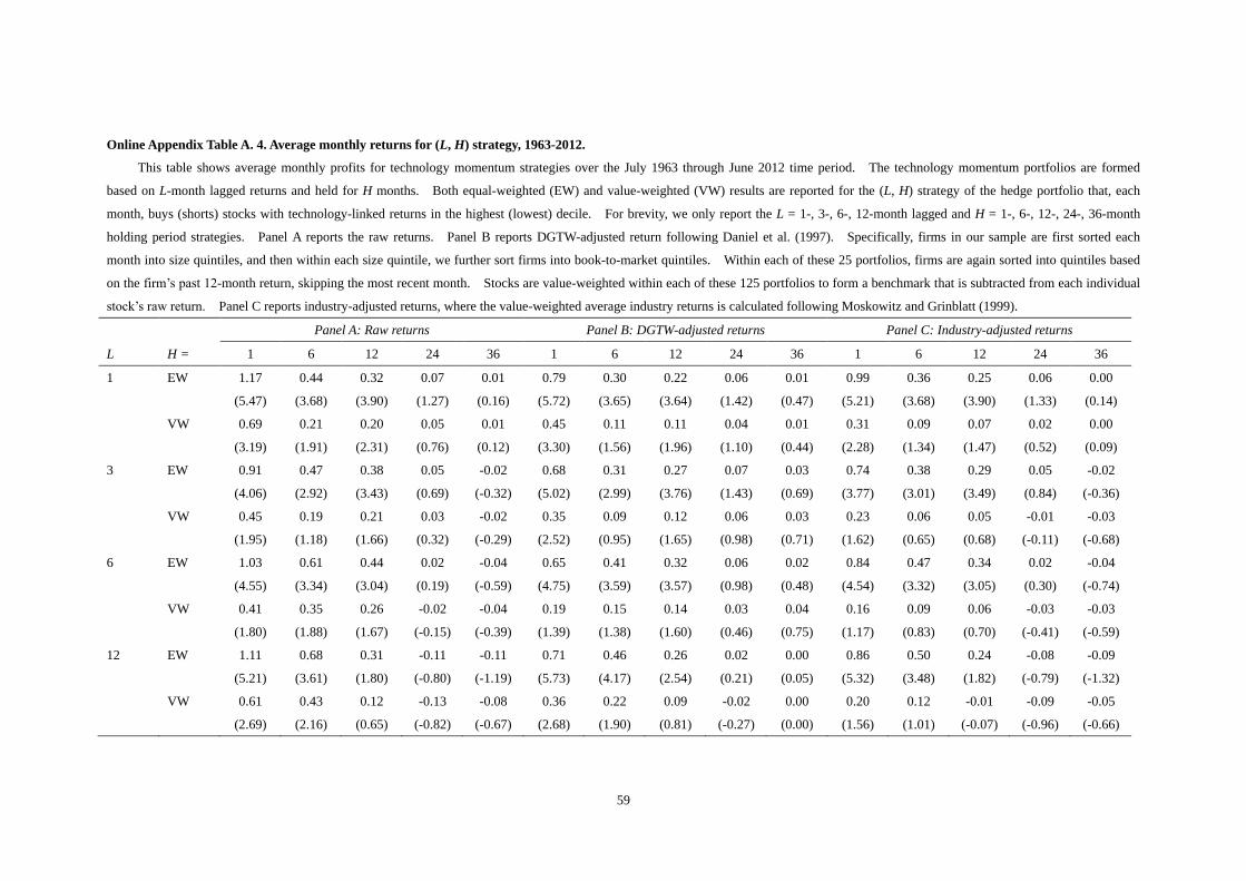
59
Online Appendix Table A. 4. Average monthly returns for (L, H) strategy, 1963-2012.
This table shows average monthly profits for technology momentum strategies over the July 1963 through June 2012 time period. The technology momentum portfolios are formed
based on L-month lagged returns and held for H months. Both equal-weighted (EW) and value-weighted (VW) results are reported for the (L, H) strategy of the hedge portfolio that, each
month, buys (shorts) stocks with technology-linked returns in the highest (lowest) decile. For brevity, we only report the L = 1-, 3-, 6-, 12-month lagged and H = 1-, 6-, 12-, 24-, 36-month
holding period strategies. Panel A reports the raw returns. Panel B reports DGTW-adjusted return following Daniel et al. (1997). Specifically, firms in our sample are first sorted each
month into size quintiles, and then within each size quintile, we further sort firms into book-to-market quintiles. Within each of these 25 portfolios, firms are again sorted into quintiles based
on the firm’s past 12-month return, skipping the most recent month. Stocks are value-weighted within each of these 125 portfolios to form a benchmark that is subtracted from each individual
stock’s raw return. Panel C reports industry-adjusted returns, where the value-weighted average industry returns is calculated following Moskowitz and Grinblatt (1999).
Panel A: Raw returns Panel B: DGTW-adjusted returns Panel C: Industry-adjusted returns
L H = 1 6 12 24 36 1 6 12 24 36 1 6 12 24 36
1 EW 1.17 0.44 0.32 0.07 0.01 0.79 0.30 0.22 0.06 0.01 0.99 0.36 0.25 0.06 0.00
(5.47) (3.68) (3.90) (1.27) (0.16) (5.72) (3.65) (3.64) (1.42) (0.47) (5.21) (3.68) (3.90) (1.33) (0.14)
VW 0.69 0.21 0.20 0.05 0.01 0.45 0.11 0.11 0.04 0.01 0.31 0.09 0.07 0.02 0.00
(3.19) (1.91) (2.31) (0.76) (0.12) (3.30) (1.56) (1.96) (1.10) (0.44) (2.28) (1.34) (1.47) (0.52) (0.09)
3 EW 0.91 0.47 0.38 0.05 -0.02 0.68 0.31 0.27 0.07 0.03 0.74 0.38 0.29 0.05 -0.02
(4.06) (2.92) (3.43) (0.69) (-0.32) (5.02) (2.99) (3.76) (1.43) (0.69) (3.77) (3.01) (3.49) (0.84) (-0.36)
VW 0.45 0.19 0.21 0.03 -0.02 0.35 0.09 0.12 0.06 0.03 0.23 0.06 0.05 -0.01 -0.03
(1.95) (1.18) (1.66) (0.32) (-0.29) (2.52) (0.95) (1.65) (0.98) (0.71) (1.62) (0.65) (0.68) (-0.11) (-0.68)
6 EW 1.03 0.61 0.44 0.02 -0.04 0.65 0.41 0.32 0.06 0.02 0.84 0.47 0.34 0.02 -0.04
(4.55) (3.34) (3.04) (0.19) (-0.59) (4.75) (3.59) (3.57) (0.98) (0.48) (4.54) (3.32) (3.05) (0.30) (-0.74)
VW 0.41 0.35 0.26 -0.02 -0.04 0.19 0.15 0.14 0.03 0.04 0.16 0.09 0.06 -0.03 -0.03
(1.80) (1.88) (1.67) (-0.15) (-0.39) (1.39) (1.38) (1.60) (0.46) (0.75) (1.17) (0.83) (0.70) (-0.41) (-0.59)
12 EW 1.11 0.68 0.31 -0.11 -0.11 0.71 0.46 0.26 0.02 0.00 0.86 0.50 0.24 -0.08 -0.09
(5.21) (3.61) (1.80) (-0.80) (-1.19) (5.73) (4.17) (2.54) (0.21) (0.05) (5.32) (3.48) (1.82) (-0.79) (-1.32)
VW 0.61 0.43 0.12 -0.13 -0.08 0.36 0.22 0.09 -0.02 0.00 0.20 0.12 -0.01 -0.09 -0.05
(2.69) (2.16) (0.65) (-0.82) (-0.67) (2.68) (1.90) (0.81) (-0.27) (0.00) (1.56) (1.01) (-0.07) (-0.96) (-0.66)