introduction - upemperso-math.univ-mlv.fr/users/seuret.stephane/cimpa_course.pdf · multifractal...

MULTIFRACTAL ANALYSIS AND WAVELETS

STEPHANE SEURET

Abstract. In this course, we give the basics of the part of multifractaltheory that intersects wavelet theory. We start by characterizing thepointwise Holder exponents by some decay rates of wavelet coefficients.Then, we give some examples of wavelet series having a multifractalbehavior, and we explain how to build wavelet series with prescribedpointwise Holder exponents. Next we develop the problematics of mul-tifractal formalism, going from the intuitive formula by Frisch and Parisito explicit and exploitable formulas. We prove that ”multifractals areeverywhere”, in the sense that typical functions in Besov spaces or typ-ical measures are multifractal in the sense of Baire’s categories. Wefinish by some well-known examples of multifractal wavelet series, ran-dom and deterministic, focusing on the influence of certain adaptivethreshold procedures to the multifractal properties of signals.

1. Introduction

In the context of functional analysis, multifractal analysis is concernedwith the local regularity and the scaling behavior of functions: it is an at-tempt to describe the geometric and statistic distribution of the singularitiesof a function. One major motivation for going inside multifractal theory isthat multifractal studies have direct connections with many mathematicalfields (harmonic and functional analysis, probability theory and stochasticprocesses, dynamical systems and ergodic theory, geometric measure the-ory and even number theory), and simultaneously they have many naturalapplication fields (physics, biology and physiology, amongst many other up-coming examples) based on the developments of new numerical proceduresin signal and image processing.

In this course, I develop the basic facts about multifractal analysis offunctions, the tools being mainly geometric measure theory and wavelets.

Let us start by recalling how the local regularity of a locally boundedfunction is quantified.

Definition 1.1. Let f ∈ L∞loc(Rd), and x0 ∈ Rd. Let α ∈ R+ \ N.The function f is said to belong to Cα(x0) if there exist two positive

constants C > 0, M > 0, a polynomial P with degree less than bαc (theinteger part of α), such that when |x− x0| ≤M ,

(1) |f(x)− P (x− x0)| ≤ C|x− x0|α.

Date: March 10, 2014.

1

2 STEPHANE SEURET

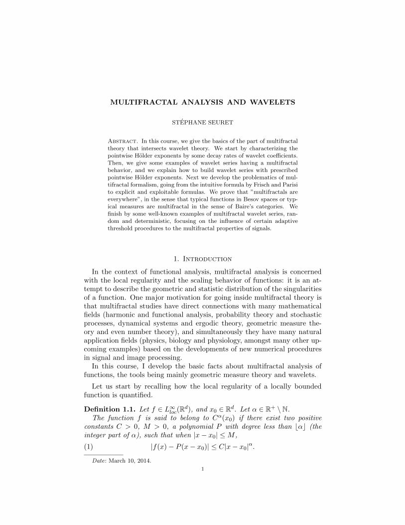
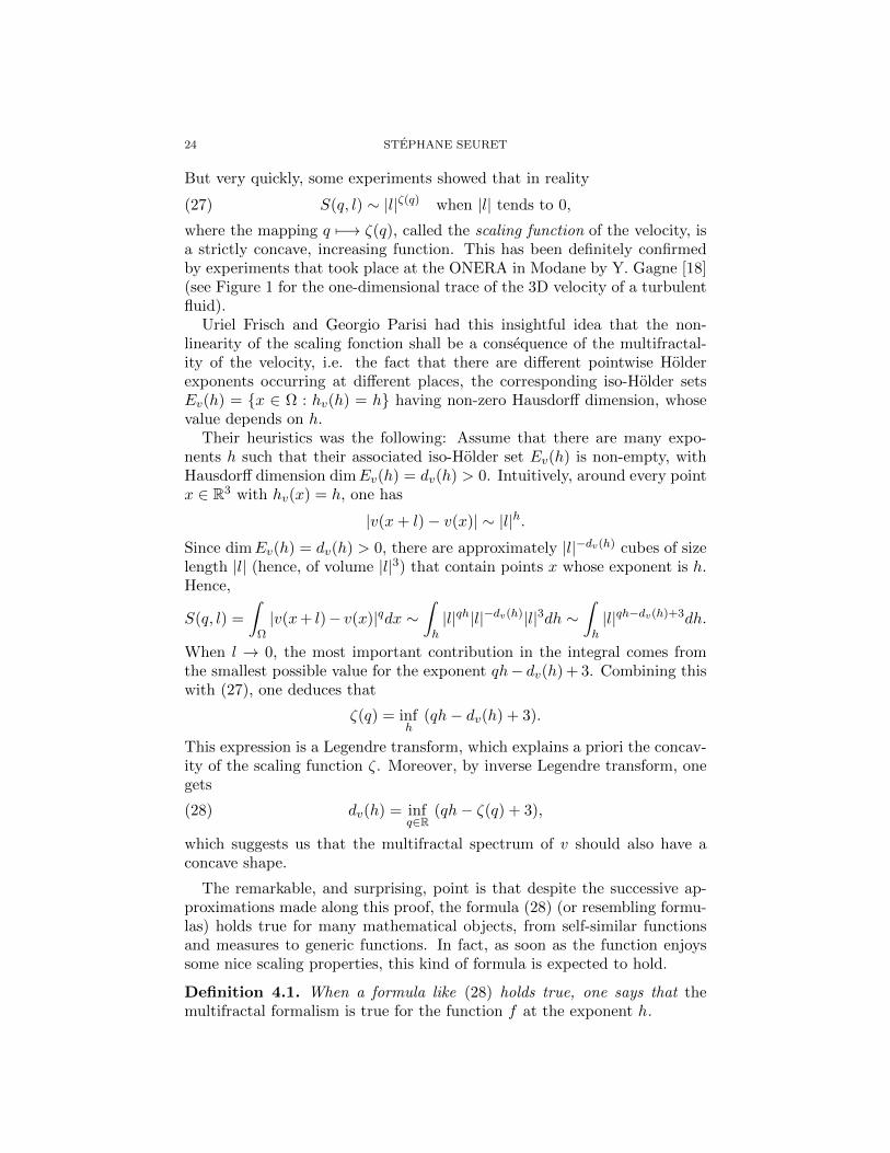
Figure 1. 1D-signal of the velocity of a turbulent fluid [18].

Then, the pointwise Holder exponent of f at x is

(2) hf (x0) = supα ≥ 0 : f ∈ Cα(x0),If hf (x0) = h, the point x0 is called a singularity of order h for f .

Observe that when the exponent hf (x0) is strictly less than 1, it takes amuch simpler form:

hf (x0) = lim infx→x0

log |f(x)− f(x0)|log |x− x0|

,

where by convention log 0 = −∞.

Exercise 1.1. Prove that the polynomial P in the definition of Cs(x) isunique.

Exercise 1.2. Prove that if s < s′, Cs′(x) ⊂ Cs(x).

Exercise 1.3. Let f ∈ Cs(x), and call F a primitive of f . Prove thatF ∈ Cs+1(x). Build an example where hf (x) = s and hF (x) = s+ 2.

Exercise 1.4. Let f ∈ Cs(x), with s > 1. Do one always have f ′ ∈Cs−1(x)?

This exponent hf (x) encapsulates significant information about the localbehavior of f around x: the less its value is, the more irregular the graph ofthe function f locally looks like.

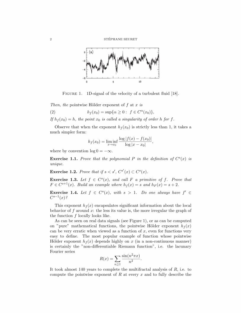
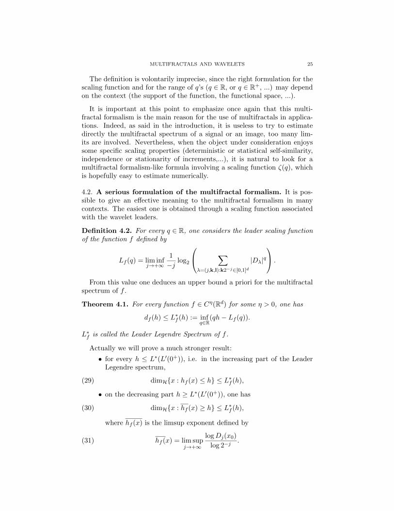
As can be seen on real data signals (see Figure 1), or as can be computedon ”pure” mathematical functions, the pointwise Holder exponent hf (x)can be very erratic when viewed as a function of x, even for functions veryeasy to define. The most popular example of function whose pointwiseHolder exponent hf (x) depends highly on x (in a non-continuous manner)is certainly the ”non-differentiable Riemann function”, i.e. the lacunaryFourier series

R(x) =∑n≥1

sin(n2πx)

n2.

It took almost 140 years to complete the multifractal analysis of R, i.e. tocompute the pointwise exponent of R at every x and to fully describe the

MULTIFRACTALS AND WAVELETS 3

1.2657

-1.26570 2

3/40

1

d (h)

h1/2

R

3/2

Figure 2. ”Non-differentiable” Riemann function, and itsmultifractal spectrum.

geometric distribution of these singularities!! The graph of R is plottedFigure 2.

Even if one is able to compute the pointwise Holder exponent of a functionf at every point x, the knowledge of all these exponents does not necessarilygive a concrete idea of what the graph of the function looks like, or of whichthe most significant singularities (or the most frequent ones) are. In orderto describe the diversity of the local behaviors of f , one focuses on theiso-Holder sets associated with the pointwise Holder exponents.

Definition 1.2. For every h ∈ R+ ∪+∞, the iso-Holder set Ef (h) is theset

Ef (h) = x ∈ Rd : hf (x) = hof all singularities of pointwise Holder exponent for f equal to h.

A single iso-Holder set Ef (h) may be concentrated around one region of

Rd, or spread all over the space. One thus needs a way to compare thesizes of the sets Ef (h). It turns out that the right notion to distinguishthem in the Hausdorff dimension, the main reason being the following: ifone keeps in mind that the models we are interested in are built usingprocedures involving either random construction or dynamical systems, thenour intuition (based on the law of large numbers or the Birkhoff ergodictheorem, depending on the context) makes us expect that there is a singlevalue hs such that Lebesgue-almost every point x ∈ Rd has a pointwiseHolder exponent hs for f (the same value hs for Lebesgue every x!). Sothe Lebesgue measure is not the appropriate tool to measure the size of theiso-Holder sets, since one Ef (h) will have full Lebesgue measure, and all theother ones will have measure 0. It is natural idea to compare their ”fractal”dimension. Actually, ”fractal” dimension does not exist, it is either box (alsocalled Minkowski) dimension, Hausdorff dimension or less frequently packingdimension. It appears that for many natural functions or sample paths ofstochastic processes, the sets Ef (h) are fractal (whatever this means!) andoften dense in the support of the corresponding function. Unfortunately,the box dimension gives full dimension (i.e. dimension d) to any dense set,so it does not distinguish them. This is one of the heuristic reasons that

4 STEPHANE SEURET

X

0 hh

dim(E (h ))X o

o

d

d (h)

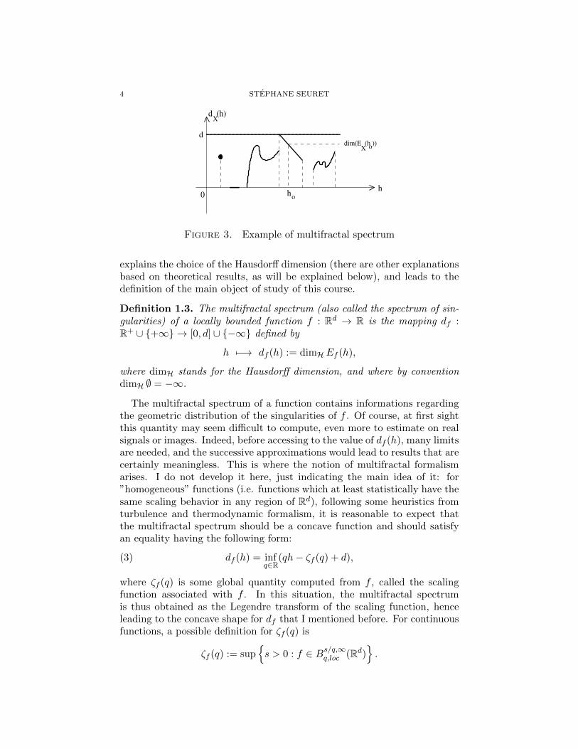
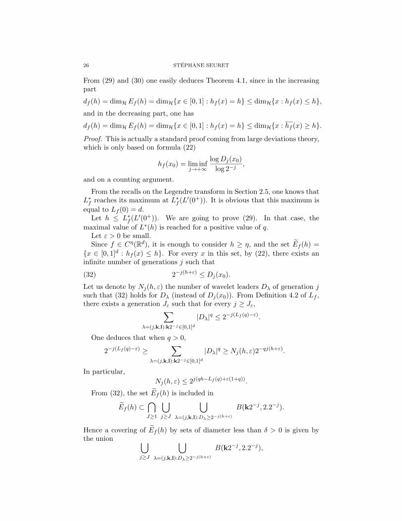
Figure 3. Example of multifractal spectrum

explains the choice of the Hausdorff dimension (there are other explanationsbased on theoretical results, as will be explained below), and leads to thedefinition of the main object of study of this course.

Definition 1.3. The multifractal spectrum (also called the spectrum of sin-gularities) of a locally bounded function f : Rd → R is the mapping df :R+ ∪ +∞ → [0, d] ∪ −∞ defined by

h 7−→ df (h) := dimHEf (h),

where dimH stands for the Hausdorff dimension, and where by conventiondimH ∅ = −∞.

The multifractal spectrum of a function contains informations regardingthe geometric distribution of the singularities of f . Of course, at first sightthis quantity may seem difficult to compute, even more to estimate on realsignals or images. Indeed, before accessing to the value of df (h), many limitsare needed, and the successive approximations would lead to results that arecertainly meaningless. This is where the notion of multifractal formalismarises. I do not develop it here, just indicating the main idea of it: for”homogeneous” functions (i.e. functions which at least statistically have thesame scaling behavior in any region of Rd), following some heuristics fromturbulence and thermodynamic formalism, it is reasonable to expect thatthe multifractal spectrum should be a concave function and should satisfyan equality having the following form:

(3) df (h) = infq∈R

(qh− ζf (q) + d),

where ζf (q) is some global quantity computed from f , called the scalingfunction associated with f . In this situation, the multifractal spectrumis thus obtained as the Legendre transform of the scaling function, henceleading to the concave shape for df that I mentioned before. For continuousfunctions, a possible definition for ζf (q) is

ζf (q) := sups > 0 : f ∈ Bs/q,∞

q,loc (Rd).


Of course the precise value of the scaling function ζf (q) may depend on thecontext, nevertheless, in all cases, when formula (3) (or an analog of it) holdstrue for a function f and an exponent h, one says that the multifractalformalism holds for f at h. See Section 4 for all details.

The intuition that the multifractal formalism holds for nice models issupported by numerous representative examples: many stochastic processes(Levy processes, wavelet series, ...) obey the multifractal formalism, aswell as ”typical” functions in many functional spaces (the set of monotonefunctions, Holder and Besov spaces for instance). Moreover, even if themultifractal formalism does not hold, the Legendre spectrum

ζ∗f (h) := infq∈R

(qh− ζf (q) + d)

is meaningful since it encapsulates information about the histograms of os-cillations or of wavelet coefficients associated with f . The key point is thatthe scaling function ζf (q) as we defined it just above, and thus its Legendretransform ζ∗f (h), is accessible by numerical methods (using log-log diagrams

for instance), while df is not. Hence, the Legendre spectrum ζ∗f (h) is aquantity that can be estimated on every signal or image, and its form canbe interpreted in terms of presence/relevance/density of the singularities ofthe object under consideration. The reader is referred to the course of P.Abry and S. Jaffard in the same volume to learn about efficient numericalprocedures to estimate various scaling functions (see also [1, 2]).

Wavelets constitute a natural tool to study the multifractal nature of afunction. For, there are two main reasons: the first one is that the pointwiseHolder exponent can be characterized by size estimates on the wavelet co-efficients (see Theorem 3.1 below). The second one is that many functionalspaces (Holder and Besov spaces for instance) can also be characterized bydecay rates of the wavelet coefficients. Also, the fact that a wavelet basisis self-similar by construction (all the functions ψj,k = 2j/2ψ(2jx − k) areobtained through a translation and dilation of a same initial function ψ) is apriori an advantage to study ”fractal”-like properties, but this could be dis-cussed since it is self-similar with very specific ratio (powers of 2) while oneaims at studying any irregular function. Anyway, wavelets are very impor-tant tools in this course, and some prior knowledge about their constructionis advised, although we will only use their basic properties (vanishing mo-ments, space and frequency localization).

The course is organized as follows. Section 2 contains the necessary mate-rials for the rest of the course: wavelet coefficients, Hausdorff dimension andsome geometric measure theory, local dimensions of measures. In Section 3,I prove the characterization of the pointwise Holder exponent by size esti-mates of the wavelet coefficients, or by size estimates of the wavelet leaders.I also explain how to build a function with prescribed local regularity, andgive some examples of multifractal wavelet series. In Section 4, I developthe intuitive notion of multifractal formalism, and then give some theoretical

6 STEPHANE SEURET

results on multifractals; for instance I explain how to obtain a priori upperbounds for multifractal spectra for Besov function and measures. In Section5 it is proved that typical functions or measures (in the sense of Baire’s cat-egory) in suitable functional spaces are multifractal. There, I use methodsdescribed in Section 2 to effectively compute the Hausdorff dimensions ofthe iso-Holder sets of some functions. Finally Section 6 contains examplesof multifractal functions built as wavelet series (the proofs are essentiallywritten as long exercises).

2. Recalls on wavelets and geometric measure theory

2.1. Wavelets. I recall very briefly the basics of multiresolution waveletanalysis (for details see for instance [34, 15]). For an arbitrary integer N ≥1 one can construct compactly supported functions Ψ0 ∈ CN (R) (calledthe scaling function) and Ψ1 ∈ CN (R) (called the mother wavelet), withΨ1 having at least N + 1 vanishing moments (i.e.

∫R x

nΨ1(x)dx = 0 forn ∈ 0, . . . , N), and such that the set of functions

Ψ1j,k : x 7→ Ψ1(2jx− k)

for j ∈ Z, k ∈ Z form an orthogonal basis of L2(R) (note that we choose theL∞ normalization, not L2). In this case, the wavelet is said to be N -regular.

Let us introduce the notations

0d := (0, 0, · · · , 0), 1d := (1, 1, · · · , 1), Ld = 0, 1d\0d.An orthogonal basis of L2(Rd) is then obtained by tensorization. For

every λ = (j,k, l) ∈ Z× Zd × Ld, let us define the tensorized wavelet

Ψλ(x) = Ψl(2jx− k) :=d∏i=1

Ψlij,ki

(xi),

with obvious notations: k = (k1, k2, · · · , kd) and l = (l1, l2, · · · , ld).Any function f ∈ L2(Rd) can be written (the equality being true in

L2(Rd))

(4) f(x) =∑

λ=(j,k,l): j∈Z,k∈Zd, l∈LddλΨλ(x),

where

(5) dλ = dλ(f) := 2jd∫Rdf(x)Ψλ(x) dx.

It is implicit in (5) that the wavelet coefficients depend on f . Observe thatin the wavelet decomposition (4), no wavelet Ψλ such that l = 0d (whereλ = (j,k, l)) appears.

Assumption: We always assume that the wavelet has a number of van-ishing moments larger than the index of regularity that we are looking at.Typically, if we focus on singularities on order h, we assume that Ψ1 has atleast bhc+ 1 vanishing moments.


The reason for this assumption is that wavelets with enough vanishingmoments can be used to characterize Holder functions.

Theorem 2.1. For s ∈ R+\N, a function f belongs to Cs(Rd) if and onlyif there exists a constant C > 0 such that

(6) ∀λ ∈ Z× Zd × 0, 1d |dλ(f)| ≤ C2−js.

I do not prove Theorem 2.1 here, it is a good exercise, the proof of whichcan be achieved by adapting the proof of Theorem 3.1 given later.

Wavelets can also be used to characterize functions in a Besov space, seeSection 4.3.

2.2. Localization of the problem. We are interested in the local behav-ior of functions, hence when focusing on a point x0 ∈ Rd, what happens farfrom x0 should not interfere with our questions. Moreover, again becausewe concentrate on local phenomena, the low frequency terms have no im-portance in our analysis. This is why we focus only on functions supportedby [0, 1]d, and when we deal with wavelets, we assume that the function wedeal with have a wavelet decomposition like

(7) f =∑

λ=(j,k,l):

j≥0,k2−j∈[0,1]d, l∈Ld

dλΨλ(x).

2.3. Hausdorff and box dimension. Two notions of dimensions of setsin Rd will be used below: the Hausdorff dimension and the upper box di-mension. We recall them quickly.

Let X be a bounded set in Rd. For every ε > 0, denote by Nε(X) theminimal number of balls of diameter ε needed to fully cover the set X. Thelower box dimension of X, denoted by dimB(X), is then the real number∈ [0, d] defined as

(8) dimB(X) = lim infε→0+

logNε(X)

− log ε.

Similarly, the upper box dimension of X is

(9) dimB(X) = lim supε→0+

logNε(X)

− log ε.

Exercise 2.1. Prove that Nε(X) is well-defined, and that dimB(X) ≤ d.

Exercise 2.2. Build a set X such that dimB(X) < dimB(X)

When dimB(X) = dimB(X), one denotes by dimB(X) their commonvalue.

Exercise 2.3. Prove that:

(1) the box dimension of an open set is d.(2) the box dimension of the triadic Cantor set is log 2/ log 3.

8 STEPHANE SEURET

(3) the box dimension of a set X dense in [0, 1]d is d.

I also recall the definition of the Hausdorff dimension.

Definition 2.1. Let s ≥ 0. The s-dimensional Hausdorff measure of a setX, Hs(X), is defined as

Hs(X) = limr0Hsr(X), with Hsr(X) = inf

∑i

|Xi|s,

the infimum being taken over all the countable families of sets Xi such that|Xi| ≤ r and X ⊂

⋃iXi. Then, the Hausdorff dimension of X, dimH X, is

defined as

dimH X = infs ≥ 0 : Hs(X) = 0 = sups ≥ 0 : Hs(X) = +∞.

It is a good exercise to prove that for any bounded set E ⊂ Rd, we have

0 ≤ dimH(E) ≤ dimB(E) ≤ d.

In order to find an upper bound for the Hausdorff dimension of X, themost common method is the following: First guess what the dimensionshould be, call δ this expected value. Then, fix s > δ, and find a covering(Xi)i∈N of X such that

Hs(⋃i∈N

Xi

)< +∞.

This implies, by the definition of dimH X, that s ≥ dimHX. This beingtrue for any s > δ, one deduces that δ ≥ dimHX, hence the upper bound.

Obtaining a lower bound is in most cases much more difficult. Let usmention the mass distribution principle, on which most methods are based.

Theorem 2.2. Let X ⊂ Rd be a borelian set, and assume that there existsa positive finite measure µ supported by X satisfying the following scalingproperty: there exists a positive real number s > 0 and a constant C > 0such that

for any x ∈ X, for any 0 < r < 1, µ(B(x, r)) ≤ Crs.

Then Hs(X) > µ(X)C , and thus dimHX ≥ s.

Exercise 2.4. Prove that the Hausdorff dimension of the triadic Cantor setis log 2/ log 3 (Hint: apply Theorem 2.2 with the uniform measure on theCantor set).

Another theorem that often allows one to compute Hausdorff dimensionof iso-Holder sets in multifractal analysis is the following theorem by Beres-nevich and Velani [11]:


Theorem 2.3. Let (xn)n≥1 be a sequence of points in [0, 1]d, and let (ln)n≥1

be a positive non-increasing sequence of radii. If

Ld(

lim supn→+∞

B(xn, ln))

= Ld(

[0, 1]d),

(Ld is the d-dimensional Lebesgue measure), then for every ξ > 1, one has

Hd/ξ(

lim supn→+∞

B(xn, (ln)ξ))

= +∞.

Exercise 2.5. Let ξx be the approximation rate of an irrational numberx ∈ [0, 1] by the dyadic numbers, defined by

ξx = supξ ≥ 0 : |x− k2−j | ≤ 2−jξ for i.m. couples (j, k), j ≥ 1, k odd.

(1) Prove that for every irrational number x ∈ [0, 1], ξx ≥ 1.(2) Let Sξ = x : |x−k2−j | ≤ 2−jξ for i.m. couples (j, k), j ≥ 1, k odd

and Sξ = x : ξx = ξ. Prove that

Sξ =

⋂ξ′<ξ

Sξ′

\⋃ξ′>ξ

Sξ′

.

(3) Prove that for ξ ≥ 1, dimH(Sξ) ≤ 1/ξ and dimH(Sξ) ≤ 1/ξ.

(4) Prove that for ξ > 1, H1/ξ(Sξ) = H1/ξ(Sξ) = +∞.

(5) Deduce the value of the Hausdorff dimension of Sξ and Sξ, for everyξ ≥ 1.

Exercise 2.6. Let ξx be the Diophantine approximation rate of an irrationalnumber x ∈ [0, 1] by the rationals, defined by

ξx = supξ ≥ 0 : |x−p/q| ≤ q−2ξ for infinitely many q ≥ 1 and p with p ∧ q = 1.

(1) Prove Dirichlet’s theorem: for every irrational number x ∈ [0, 1],ξx ≥ 1. (Hint: Use a counting argument).

(2) Let Sξ = x : |x−p/q| ≤ q−2ξ for infinitely many q ≥ 1 and p with p ∧ q = 1and Sξ = x : ξx = ξ. Prove that

Sξ =

⋂ξ′<ξ

Sξ′

\⋃ξ′>ξ

Sξ′

.

(3) Prove that for ξ ≥ 1, dimH(Sξ) ≤ 1/ξ and dimH(Sξ) ≤ 1/ξ.

(4) Prove that for ξ > 1, H1/ξ(Sξ) = H1/ξ(Sξ) = +∞.

(5) Deduce the value of the Hausdorff dimension of Sξ and Sξ, for everyξ ≥ 1.

Other methods will be probably used hereafter, I will mention them alongthe proofs.

10 STEPHANE SEURET

2.4. Local dimensions of measures. Recall that the support of a Borelpositive measure, denoted by Supp(µ), is the smallest closed set E ∈ Rdsuch that µ(Rd \ E) = 0.

Definition 2.2. Let µ be a positive measure supported on Rd at x0 ∈Supp(µ). The (lower) local dimension hµ(x0) (also called local Holder expo-nent) is

(10) hµ(x0) = lim infr→0+

logµ(B(x0, r))

log r,

where B(x0, r) denotes the open ball with center x0 and radius r. When x0 /∈Supp(µ), by convention we set hµ(x0) = +∞.

Of course, in R, there is a correspondence between the local dimension ofa measure and the pointwise Holder exponent of its primitive F (x) =

∫ x0 dµ.

Exercise 2.7. Prove that if hµ(x0) /∈ N, then hF (x0) = hµ(x0). Is theconverse true? (Hint: consider the Lebesgue measure).

Iso-Holder sets and multifractal spectrum are quantities that can be de-fined for measures using the same ideas: One sets

Eµ(h) = x ∈ Rd : hµ(x) = hand

dµ : h 7−→ dµ(h) := dimHEµ(h).

Contrarily to what happens for measures, there is a strong constraintvalid for all measures: for every h ≥ 0, for every positive Borel measure onRd, one has (see next Sections)

dµ(h) ≤ min(h, d).

This is one major difference between measures and functions from the mul-tifractal standpoint (essentially due to the fact that measures have boundedvariations).

2.5. Legendre transform. The Legendre transform appears in many placesin analysis, I recall the properties that are needed in the following.

Definition 2.3. Let L : R → R be a concave increasing function. TheLegendre transform of L is the mapping L∗ : R→ R ∪ −∞ defined by

h 7→ L∗(h) := infq∈R

(qh− L(q)

).

The assumption that L is increasing is not necessary for the definitionof the Legendre transform, but it will be the case in our context in thefollowing. In our cases, the function L satisfies L(0) < 0, and in this caseone shall keep in mind the following properties:

• The support of L∗ is included in the smallest interval containingL′(R), the extreme points may or may not belong to the support,depending on L.


• L∗ is concave on its support.• If h = L′(q) (i.e. L is differentiable at q), then L∗(h) = qh− L(q).• When L′(0+) exists, the Legendre transform L∗ reaches its maximum

at h = L′(0+), and L∗(L′(0+)) = −L(0).• L∗ is increasing on the interval when h ≤ L′(0+), and is decreasing

when h ≥ L′(0+) (again, the extreme points may not belong to thesupport).

I draw the attention of the reader that L is not necessarily continuouslydifferentiable, and that difficulties may appear to find the precise rangeof real numbers h such that L∗(h) ≥ 0. These problems occur in manycontexts, too numerous to list them in details now.

Exercise 2.8. Prove each of the preceding items.

3. Pointwise Holder exponent

3.1. Characterization by decay rate of wavelet coefficients. Recallthe Definition 2 of the pointwise Holder exponent of a locally bounded func-tion f at a point x0 ∈ Rd. The definition of hf (x) involves some functionalspaces Cs(x), which can be (almost) characterized by the decay rate of thecoefficients located around x0, as stated by the next theorem of Jaffard [23].

Theorem 3.1. Let s ∈ R+ \ N, and let f ∈ L2(Rd).Assume that f belongs to Cs(x0). Then, there exist two constants M > 0

and C > 0 such that for every λ = (j,k, l) such that j ≥ 0, |x0−k2−j | ≤M ,and for every l ∈ Ld, one has

(11) |dλ| ≤ C(2−j + |x0 − k2−j |)s.

Reciprocally, if the wavelet coefficients of a function f ∈⋂ε>0

Cε([0, 1]d) sat-

isfies (11), then f ∈ Cslog(x0).

Recall that f ∈ Cslog(x0) when locally around x0, there exists a polynomial

P of degree less than bsc such that

(12) |f(x)− P (x− x0)| ≤ C|x− x0|s| log |x− x0||.As usual, the symbol A . B means that inequality A ≤ CB holds for

some constant C independent of the parameters involved in the formula.

Proof. We start by the direct implication. Assume that f ∈ Cs(x0), andlet us call P the unique polynomial such that if |x− x0| ≤ M (for someconstant M), (1) holds true.

Fix λ = (j,k, l) such that j ≥ 0 and

(13) |x0 − k2−j | ≤ M := M/2.

One has

dλ = 2dj∫Rdf(x)Ψλ(x)dx = 2dj

∫Rd

(f(x)− P (x− x0))Ψλ(x)dx,

12 STEPHANE SEURET

where we used the vanishing moments up to the order bsc to introduce thepolynomial in the integral. Then,

|dλ| ≤ 2dj∫|x−x0|≤M

|f(x)− P (x− x0)||Ψλ(x)|dx

+2dj∫|x−x0|≥M

|f(x)||Ψλ(x)|dx

+2dj∫|x−x0|≥M

|P (x− x0)||Ψλ(x)|dx.

Let us call IM , JM and KM the last three terms. Using (1), the first termis bounded above by

IM . 2dj∫|x−x0|≤M

|x− x0|s|Ψl(2jx− k)|dx

.∫|u|≤M2j

|2−j(u+ k)− x0|s|Ψl(u)|du.

Since each Ψλ is continuous and compactly supported, say, with supportincluded in [−M ′,M ′]d, it is uniformly bounded (independently of λ, due tothe choice of the L∞-normalization for the wavelet’s family) and one gets

IM .∫

[−M ′,M ′]d|2−j(u+ k)− x0|sdu

.∫

[−M ′,M ′]d|2−ju|s + |x0 − k2−j |sdu

. (2−js + |x0 − k2−j |s) . (2−j + |x0 − k2−j |)s,where we used the double-sided inequality (x+y)s ≤ 2s(xs+ys) ≤ 2s+1(x+y)s.

Let us now treat the second term. By the Cauchy-Schwarz inequality andusing that f ∈ L2(Rd), one obtains

JM . 2dj

(∫|x−x0|≥M

|f(x)|2dx

)1/2(∫|x−x0|≥M

|Ψλ(x)|2dx

)1/2

. 2dj

(∫|x−x0|≥M

|Ψl(2jx− k)|2dx

)1/2

. 2dj/2

(∫|2−j(u+k)−x0|≥M

|Ψl(u)|2du

)1/2

.(14)

Observe that our choice (13) for λ imposes that

(15) u : |2−j(u+ k)− x0| ≥M ⊂ u : |u| ≥ M2j.The wavelets Ψ0 and Ψ1 being compactly supported, (15) tells us that theintegral in (14) is 0 for j large enough.


The third term is treated almost similarly. The polynomial P being ofdegree at most bsc, one can write

KM . 2dj

∫|x−x0|≥M

(|P (x− x0)|

1 + |x− x0|s+d+2

)2

dx

1/2

×

(∫|x−x0|≥M

(1 + |x− x0|s+d+2)2|Ψλ(x)|2dx

)1/2

. 2dj∥∥∥∥ |P (.)|

1 + |.|s+d+2

∥∥∥∥L2(Rd)

×

(∫|x−x0|≥M

(1 + |x− x0|s+d+2)2|Ψl(2jx− k)|2dx

)1/2

. 2dj/2

(∫|u|≥M2j

(1 + |2−j(u+ k)− x0|s+d+2)2|Ψl(u)|2du

)1/2

.

where (15) has been used. Again, the last integral is zero when j becomeslarge. Hence the first assertion.

Exercise 3.1. Prove that the same holds when the wavelets are not com-pactly supported (Hint: use their rapid decay at infinity).

Let us move to the reciprocal, which is more delicate to handle with.Assume that (11) holds for every λ = (j,k, l) such that j ≥ 0, |x0 −

k2−j | ≤M , and l ∈ Ld.We start from the decomposition (7). Since each Ψλ is at least Cbsc+1(Rd),

this is also true for every function fj defined as the sum over each fixedgeneration j of the wavelet coefficients of f , i.e.

(16) fj(x) =∑

λ=(j,k,l): k2−j∈[0,1]d, l∈LddλΨλ(x),

The partial derivatives of fj are: for every α := (α1, ..., αd) ∈ Nd such that|α| := α1 + ...+ αd ≤ bsc+ 1, one has

∂αfj(x) =∑

λ=(j,k,l): k2−j∈[0,1]d, l∈Lddλ ∂

αΨλ(x),

Each partial derivative of Ψ0 and Ψ1 is compactly supported, hence theysatisfy the inequalities for all v ∈ Rd

(17) |∂αΨl(v)| ≤ C

1 + |v|2s+2d+4

14 STEPHANE SEURET

where the constant C is uniform in α ranging in the set of indices such that|α| ≤ bsc+ 1. Since Ψλ(x) = Ψl(2jx− k), the last upper bound yields

|∂αΨλ(x)| ≤ C2j|α|

1 + |2jx− k|2s+2d+4.

From this we deduce that

|∂αfj(x)| ≤∑

λ=(j,k,l): k2−j∈[0,1]d, l∈Ld|dλ|

C2j|α|

1 + |2jx− k|2s+2d+4,

Observe now that, up to a modification of the constant C, (11) is also true forλ = (j,k, l) such that j ≥ 0, |x0−k2−j | ≤ 1 (not only for |x0−k2−j | ≤M),since the sequence of the wavelet coefficients of f are necessarily boundedby ‖f‖L2 , thus when for all λ such that |x0 − k2−j | ≥ M , one has |dλ| ≤‖f‖L2 . |x0−k2−j |s (with uniform constants). This yields the upper bound

|∂αfj(x)| .∑

λ=(j,k,l): k2−j∈[0,1]d, l∈Ld

2j|α|(2−j + |x0 − k2−j |)s

1 + |2jx− k|2s+2d+4

.∑

λ=(j,k,l): k2−j∈[0,1]d, l∈Ld

2j|α|(2−js + |x− x0|s + |x− k2−j |s)1 + |2jx− k|2s+2d+4

.

The first two terms in the last sum are independent of k, and thus thecorresponding sums are bounded above by 2j|α|(2−js + |x− x0|s). It is easyto see that the last one satisfies∑

λ=(j,k,l): k2−j∈[0,1]d, l∈Ld

2j|α||x− k2−j |s

1 + |2jx− k|2s+2d+4. 2−j(s+d+2).

We finally get the inequality

(18) |∂αfj(x)| . 2j|α|(2−js + |x− x0|s).

Since the wavelets are compactly supported, it is easily seen that fj hassame uniform Holder regularity as Ψ0 and Ψ1, i.e. fj belongs at least to

Cbsc+1(Rd). Using the Taylor polynomial Pj of order bsc of each fj , one has

|fj(x)− Pj(x− x0)| ≤ |x− x0|bsc+1 sup|α|=bsc+1

|∂αfj(x)|

. |x− x0|bsc+12j(bsc+1)(2−js + |x− x0|s).(19)

It is time now to construct the polynomial associated with f . Obviouslyone has the decomposition f(x) =

∑j≥0 fj(x), hence it is natural to con-

sider the polynomial P =∑

j≥0 Pj as potential candidate. From the aboveestimates one easily sees that this polynomial is well defined.

We fix some x close to x0. Let us call j0 the unique integer such that

(20) 2−j0 ≤ |x− x0| < 2−j0+1.


Recall that f is supposed to belong to Cη(Rd), for some η > 0. We thenintroduce the integer

(21) j1 = bj0s

ηc > j0,

where we can assume that j1 > j0 since η can be taken as small as wewant. It remains us to bound above the difference |f(x) − P (x − x0)| bythe desired quantity, i.e. |x− x0|s| log |x− x0||. Let us split this quantityinto four terms, depending on the generations of the associated waveletdecomposition. More precisely,

f(x)− P (x− x0) =

j0∑j=0

(fj(x)− Pj(x− x0)) +

j1∑j=j0+1

fj(x)

+∑

j≥j1+1

fj(x)−+∞∑

j=j0+1

Pj(x− x0).

We call S1, S2, S3 and S4 the four sums above.First, we have by (19)

|S1| .j0∑j=0

|fj(x)− Pj(x− x0)|

.j0∑j=0

|x− x0|bsc+12j(bsc+1)(2−js + |x− x0|s)

. |x− x0|bsc+1j0∑j=0

(2j(bsc+1−s) + 2j(bsc+1)|x− x0|s

). |x− x0|bsc+1(2j0(bsc+1−s) + 2j0(bsc+1)|x− x0|s). |x− x0|s,

where the last ”miracle” follows from (20). Then, by (18) with α = 0d,

|S2| .j1∑

j=j0+1

|fj(x)| .j1∑

j=j0+1

(2−js + |x− x0|s)

. (j1 − j0)(2−j0s + |x− x0|s) . |x− x0|s| log |x− x0||,

since j1 − j0 ∼ j0(1 − s/η) ∼ log |x− x0|| by (13). Further, recalling thatthe function f ∈ Cη(Rd), the wavelet coefficients of fj satisfy |dλ| . 2−jη,one sees that ‖fj‖∞ . 2−jη (here the assumption that the wavelets arecompactly supported makes the computations easier). Hence,

|S3| .+∞∑

j=j1+1

|fj(x)| .+∞∑

j=j1+1

2−jη . 2−j1η . 2−j0s . |x− x0|s.

16 STEPHANE SEURET

Finally, each polynomial Pj has the form

Pj(x− x0) =

bsc∑n=0

∑|α|=n

cα∂αfj(x0)(x− x0)n,

for some universal coefficients cα. Hence it can be bounded above as followsusing (18)

|Pj(x− x0)| .bsc∑n=0

∑|α|=n

cα|∂αfj(x0)||x− x0|n

.bsc∑n=0

2jn|x− x0|n(2−js + |x− x0|s)

. 2jbsc|x− x0|bsc(2−js + |x− x0|s),where we used that j ≥ j0, implying 2j |x− x0| > 1. Finally,

|S4| .+∞∑

j=j0+1

|Pj(x)| .+∞∑

j=j0+1

2jbsc|x− x0|bsc(2−js + |x− x0|s) . |x− x0|s.

This concludes the proof.

Let us end this section with an important remark: Theorem 3.1 tells usthat to find the value of hf (x0), it is not enough to look at the waveletcoefficients that lie inside the ”cone of influence” around x0, i.e. the λsuch that |k2−j − x0| ≤ M2−j . The cone of influence contains the waveletcoefficients whose value is influenced by the value of f at x, and one maybelieve that they are the only ones that play a role in the value of thepointwise Holder exponent of f at x. In fact, when the largest coefficientsare located within the cone of influence of x0, x0 is a cusp.

But it may happen that coefficients located very far from the cone ofinfluence are the most important ones, in the sense the inequality (11) issaturated for the coefficients. Actually, when (11) is saturated for waveletcoefficients dλ satisfying |x− x0| ∼ 2−jρ for some ρ < 1, one can prove thatx0 is an oscillating singularity with singularity exponent 1/ρ−1 (see the nextsections for more details). So it is definitely not enough to concentrate onthe cone of influence, especially when building local regularity algorithms.This is also one main motivation for introducing wavelet leaders.

Exercise 3.2. Construct a wavelet series in R such that all its waveletcoefficients are either 0 or equal to 2−jα and such that hf (0) = 2α, hf (x) = αif x 6= 0.

Is is possible to have hf (x) = 2α if x ∈ Q, hf (x) = α if x /∈ R \Q? Whatif one inverses the values α and 2α?

Exercise 3.3. Prove that, under the same assumption, it is enough forthe reconstruction part to assume that (11) holds only for those wavelet


coefficients dλ such that the corresponding λ = (j,k, l) satisfies |x0−k2−j | ≤2−j/ log j.

Exercise 3.4. Consider the continuous wavelet transform defined for a > 0and b ∈ R and for a L2 function f : Rd → R by

Wf (b, a) =1

ad/2

∫Rdf(t)ψ

(t− ba

)dt.

Prove an analog of Theorem 3.1 for this wavelet transform.

Exercise 3.5. Consider the Riemann series

R(x) =∑n≥1

sin(πn2x)

n2.

and the wavelet ψ(x) = 1(x+i)2

.

(1) Compute the continuous wavelet transform of R, and relate it to the

Theta Jacobi function Θ(z) =∑

n∈Z eiπn2z. (Hint: use the a residue

formula.)

(2) Prove that R is at least C1/2(x) at every x (difficult).(3) To learn more about R, see [21, 20, 26, 13, 35].

Exercise 3.6. Let 0 < H < 1, and consider the Weierstrass function

WH(x) =∑n≥1

2−nH sin(2nx).

(1) Prove that WH ∈ CH(R) (Hint: directly prove that |WH(x)−WH(y)| ≤C|x− y|H .)

(2) Using a suitable wavelet ψ (for instance assuming that its Fourier

transform ψ has support in [1/2, 2]), prove that for every x ∈ R,hWH

(x) = H. Hence, WH is monofractal.

3.2. Characterization by decay rate of wavelet leaders. Wavelet lea-ders are a theoretical tool introduced by S. Jaffard in [29] essentially fornumerical reasons. The main idea comes from the fact that in multifractalanalysis (see next Section for the details), it is natural to consider sums ofwavelet coefficients like ∑

λ:|λ|=j

|dλ|q

for a varying parameter q ∈ R. In particular, as we will explain, the behav-ior of the sum when j → +∞ for q < 0 is related to the decreasing part ofthe multifractal spectrum of functions. It is thus natural to try to estimatethe values of such sums. Unfortunately numerical experiments show thatthis quantity is extremely unstable due to the presence of small wavelet co-efficients, which, when they are taken to a negative power, can be extremelylarge. Wavelet leaders have been thought to stabilize these sums, and theyare in fact related to multifractal analysis of capacities [31].

18 STEPHANE SEURET

Definition 3.1. For every λ = (j,k, l), one defines the dyadic cube Iλassociated with λ by

Iλ = [k2−j ,k2−j) := [k12−j , k12−j + 2−j)× ...× [kd2−j , kd2

−j + 2−j),

where k = (k1, ..., kd) ∈ Zd.Let f be a function of the form (7). For every λ = (j,k, l) with j ≥ 0

such that k2−j ∈ [0, 1]d, one defines the wavelet leader Dλ by

Dλ = sup

|dλ′ | : Iλ′ ⊂ ⋃i∈−1,0,1d

Iλ + i2−j

.

In other words, the wavelet leader Dλ is in fact the maximal value (inabsolute value) amongst all the wavelet coefficients dλ′ such that the cor-responding cube Iλ′ lies inside Iλ or inside one of its 3d − 1 immediateneighbors.

Exercise 3.7. Prove that for every f ∈ L2 each wavelet leader is a maximum(not only a supremum).

It is immediate that if Iλ′ ⊂ Iλ, Dλ′ ≤ Dλ. Hence, instead of havingwavelet coefficients that may be sparse, we end up with leader coefficientsthat enjoy a nice decreasing property (the set of wavelet leaders forms acapacity as a function of the dyadic cubes, i.e. a decreasing set function onthe dyadic wavelet tree). Multifractal analysis of capacities has been studiedin [31, 5] for instance.

Definition 3.2. For every x0 ∈ [0, 1]d and j ≥ 0, let us denote by λj(x0)

the unique cube (up to the value of l ∈ Ld) such that x0 ∈ λ with |λ| = j,and we set

Dj(x0) = Dλj(x0) and Ij(x0) = Iλj(x0).

We also set λj(x0) = (j,kj(x0), l) (the index l has no importance here, onlythe location matters).

The main theorem relating wavelet leaders and pointwise regularity is thefollowing.

Theorem 3.2. Let f be locally bounded of the form (7). Then

(22) hf (x0) = lim infj→+∞

logDj(x0)

log 2−j,

where log 0 = −∞ by convention.

Proof. The proof is rather quick and is based on Theorem 3.1. Let h :=hf (x0).

Let ε > 0. Inequality (11) implies that for large j, all wavelet coefficientsaround x0 satisfy

|dλ| ≤ C(2−j + |x0 − k2−j |)h−ε.


Let J ≥ 0 and λ = (J,K,L) be such that |K2−J − x0| ≤ M (the constantM being the one such that (11) holds).

Let λ′ = (j,k, l) be such that Iλ′ ⊂ Iλ + i2−J , for some i ∈ −1, 0, 1d.Obviously one has |k2−j − x0| ≤ 2 · 2−J , thus

|dλ′ | . (2−j + |x0 − k2−j |)h−ε| . 2−J(h−ε).

We deduce that |Dλ| ≤ 2−J(h−ε), and thus that

lim infj→+∞

logDj(x0)

log 2−j≥ h− ε.

Letting ε go to zero gives one inequality in (22).

Moving to the converse inequality, we know that (11) must be saturatedfor some coefficients. Let ε > 0, and consider one coefficient λ = (j,k, l)such that

|dλ| ≥ (2−j + |x0 − k2−j |)h+ε.

There are infinitely many such coefficients.Let J be the unique integer such that 2−J−1 ≤ |x0 − k2−j | < 2−J . Then,

by construction, Iλ ⊂ IJ(x0) + i2−J for some i ∈ −1, 0, 1d. This yieldsthat

DJ(x0) ≥ |dλ| ≥ (2−j + |x0 − k2−j |)h+ε ≥ 2−J(h+2ε).

Taking liming of both sides, we get

lim infj→+∞

logDj(x0)

log 2−j≤ h+ ε,

and the result follows when ε tends to zero.

Exercise 3.8. Prove that there must exist (an infinite number of) λ suchthat Dλ = |dλ|.

3.3. Prescription of Holder exponents. As said in the introduction,the exponent mapping x 7→ hf (x) of a locally bounded function may not beregular, and one may wonder what form this mapping can take. It is alsonatural, for practical purposes, to try to build functions with prescribedHolder regularity. This problem is completely solved.

Exercise 3.9. Let g be a strictly positive and continuous function. Build afunction f such that its pointwise Holder exponents are exactly hf (x) = g(x)at every x (Hint: modify the Weierstrass function WH introduced in Exercise3.6).

Proposition 3.1. Let f ∈ Cη(Rd) for some η > 0. Then the mappingx 7→ hf (x) is the liminf of a sequence of continuous functions.

Reciprocally, if (gn)n≥1 is a sequence of continuous functions satisfy-ing gn ≥ η, then there exists a function f ∈ Cη(Rd) such that hf (x) =lim infn→+∞ gn(x).

20 STEPHANE SEURET

Proof. Let us start by remarking that any function f has the same pointwiseHolder exponents everywhere as the sum f + g where g is the wavelet series

whose wavelet coefficients are all equal to ±2−j2

for j ≥ 0 (there is no needto precise how the signs are chosen). Hence, up to a modification that doesnot affect the pointwise Holder coefficients, one may assume that the wavelet

coefficients of f satisfy |dλ| ≥ 2−j2

for every j ≥ 2.Then, (11) implies that

hf (x) = lim infj→+∞,|λ|=j

log |dλ|log(2−j + |x− k2−j |)

.

Let us denote by gλ the map x 7→ log |dλ|log(2−j+|x−k2−j |) . It is obviously con-

tinuous with respect to x. Hence, hf (x) is indeed the liminf of a sequenceof continuous functions.

Reciprocally, consider a sequence (gn)n≥1 of continuous functions greaterthan η > 0. We work only on the cube [0, 1]d, the extension to Rd isimmediate by concatenation. We build iteratively a wavelet series by thefollowing method.

Let us first start by remarking that we can assume that each function gn isC1. Otherwise we replace gn by any C1 function gn such that |‖gn− gn‖∞ ≤1/2n. Then it is obvious that

g(x) = lim infn→+∞

gn(x) = lim infn→+∞

gn(x).

We first construct a sequence Jn as follows.Fix J0 = 1, and assume that Jn is found. To find Jn+1, consider gn+1.

By uniform continuity, there exists Jn+1 such that |x− y| ≤ 2−Jn+1 implies

|gn+1(x)− gn+1(y)| ≤ 2−(n+1). We also assume that

2−Jn infgn(x):x∈[0,1]d ≥ 2−Jn+1(supgn+1(x):x∈[0,1]d).

Finally, we choose Jn+1 as the integer

(23) Jn+1 = max(Jn + n, Jn+1, sup|∇gn+1(x)| : x ∈ [0, 1]).Then, we prescribe the wavelet coefficients dλ for all λ = (j,k, l) as follows:

if Jn < j < Jn+1, then dλ = 0, and if j = Jn for some n ≥ 1, one sets

dλ = 2−jgn(k2−j).

Fix x0 ∈ [0, 1]d, and recall the Definition 3.2 of λj(x0) and kj(x0). It is atrivial matter to check that our construction implies that for every Jn, forthe wavelet leader DJn(x0),

2−Jn/2n ≤ DJn(x0)

2−Jngn(k2−Jn )≤ 2Jn/2

n.

By (22), one has hf (x0) ≤ lim infn→+∞ gn(kJn(x0)2−Jn). But our construc-

tion implies that for every n, |gn(kJn(x0)2−Jn)− gn(x0)| ≤ 1/2n, hence

lim infn→+∞

gn(kJn(x0)2−Jn) = lim infn→+∞

gn(x0),


from which we deduce that hf (x0) ≤ g(x0).Conversely, by Exercise 3.3, it is enough to consider those wavelet coeffi-

cients around x0 that satisfy |x0 − k2−Jn | ≤ 2−Jn/ log Jn . One sees that forsuch a coefficient λ = (Jn,k, l),

|dλ| = 2−Jngn(k2−Jn ) ≤ 2−Jn(gn(x0)−sup|∇gn(x)|:x∈[0,1]·|x0−k2−Jn |

).

But our construction implies that

0 ≤ sup|∇gn+1(x)| : x ∈ [0, 1] · |x0 − k2−Jn | ≤ Jn2−Jn/ log Jn ,

which tends to zero when n tends to infinity. This yields

|dλ| ≤ 2 · 2−Jngn(x0)

for n large. In particular, hf (x0) ≥ lim infn→+∞ gn(x0) = g(x0). This givesthe converse inequality.

Exercise 3.10. Extend last Proposition to functions that are only continu-ous, or only with bounded variations.

I finish this section by drawing the attention of the reader that what wehave achieved for functions is not known for measures: one does not knowwhat the possible forms of the local dimension map of a measure are like.The situation is much more complicated, as proved by next exercise [12].

Exercise 3.11. Consider the local dimension mapping x 7→ hµ(x) associated

with a probability measure µ on Rd. Prove that if it is continuous on an openset Ω, then it is constant and equal to d on Ω.

3.4. Other exponents. The pointwise Holder exponent does not fully de-scribe the local behavior of a continuous function. For instance, it doesnot reflect the local oscillatory behavior: the functions f1(x) = |x|1/4 and

f2(x) = |x|1/4 sin(|x|−1) have the same exponent 1/4 at 0, but they exhibitobviously a different behavior.

There are many other local regularity exponents that allows one to distin-guish functions with the same pointwise Holder exponent. Let us mentiontwo of them.

Definition 3.3. The local Holder exponent of f at x0 is defined as

(24) hlf (x0) = limε→0

supα ≥ 0 : f ∈ Cα(B(x0, ε)),

where B(x0, ε) stands for the ball (using any norm) centered at x0 of radiusε.

Exercise 3.12. Prove that the formula (24) makes sense, and that the valuedoes not depend on the choice of the norm.

The local Holder exponent is always lower than the pointwise Holderexponent (Exercise: prove it!). This other exponent is often used whenstudying local regularity of stochastic processes, for which it is often difficultto obtain results that are valid almost surely for all points (while it is often

22 STEPHANE SEURET

easy to get an exact value for every point almost surely). For instance,for a multifractional Brownian motion (see [30, 10] for definitions), one cancompute almost surely the value of every hlf (x), and sometimes the value

of hf (x) is not known (only for every x almost surely, not almost surely forevery x: nevertheless under some conditions the pointwise Holder exponentis known everywhere almost surely).

Another exponent encapsulates the oscillatory behavior of a function.

Definition 3.4. For every ε > 0, let f ε be a fractional primitive of f oforder ε. Then the oscillating exponent of f at x0 is defined as

(25) βf (x0) = limε→0

(∂hfε(x0)

∂ε

)|ε=0

− 1.

Recall that a fractional primitive f ε of order ε of, say, a L2 function canbe defined via the formula

f ε(x) = (−∆)ε/2(f)(x),

or via its Fourier transform by

f ε(ξ) =f(ξ)

(1 + |ξ|2)ε/2.

Exercise 3.13. Prove that for every ε > 0, hfε(x0) ≥ hf (x0) + ε. Deducethat the formula (25) makes sense.

As an example, it is quite easy to see that for the functions f1 and f2

introduced at the beginning of this section, βf1(0) = 0 while βf2(0) = 1.The term sin(|x|−1) is responsible for the value βf2(0) = 1, and one canprove that the oscillatory content is indeed contained in βf (x).

When βf (x) > 0, x is called an oscillating singularity of f . It is also oftenreferred to as a chirp, on the opposite to the case where βf (x) = 0, wherethe singularity is called a cusp.

Detecting oscillatory singularities is an important issue in signal process-ing, one knows that many phenomena occur only on such points (for in-stance, dissipation of energy in turbulent fluids may be due to this kind ofsingularities).

3.5. An example. Let µ be a positive Borel probability measure on [0, 1]d.Let us construct the wavelet series Fµ by prescribing its wavelet coefficientsas follows: for every λ, we set

(26) dλ = µ(Iλ).

Assume that the measure is uniformly regular, in the sense that thereexists a constant C > 0 and an exponent hmin > 0 such that for every ballwith center x and radius 0 < r < 1, one has

µ(B(x, r)) ≤ Crhmin .

These assumptions can be weakened.


Proposition 3.2. Under the assumption above, the wavelet series Fµ con-

verges, Fµ ∈ Chmin(Rd), and for every x ∈ [0, 1]d, one has

hFµ(x) = hµ(x).

In particular, dµ ≡ dF .

Proof. I let the proof as an exercise. The idea is essentially to prove thatthere is a universal constant C > 1 such that for every x0 ∈ Supp(µ), forevery j ≥ 0, one has

C−1 ≤ Dj(x0)

µ(B(x0, 2−j))≤ C.

Exercise 3.14. Let (ξλ) be a family of i.i.d random variables with common

law the normal Gaussian law. Consider the (random) wavelet series F whosewavelet coefficients are

dλ = µ(Iλ)ξλ.

This is a random modification of (26) and of F .

(1) Prove that, almost surely, for every x, hF (x) = hF (x), and thusdF ≡ dF .

(2) Can one weaken the i.i.d. assumption on the random coefficients?(the answer is yes, but to what extend...)

Exercise 3.15. What happens if (26) is replaced by

dλ = 2−jαµ(Iλ)β

for some α, β > 0?

4. Multifractal formalism

4.1. The intuition of U. Frisch and G. Parisi. Multifractal analysisand formalism for functions were introduced by physicists in order to inter-pret some experimental observations related to Kolmogorov’s theory of fullydeveloped turbulence. Since the 1940’s, Kolmogorov emphasized the rolein fluid mechanics played by the scaling function associated with the fluid’svelocity, defined as follows. Let v(x) be the velocity at time t and positionx of a turbulent fluid contained in a bounded domain Ω. For every q ∈ R,one studies the q-th moment of v defined by

S(q, l) =

∫Ω|v(x+ l)− v(x)|qdx.

In his K41 model, Kolmogorov models the small fluctuations of the ve-locity by a fractional Brownian motion with Hurst exponent H = 1/3, forwhich one can prove S(q, l) enjoys a nice scaling behavior of the form, forevery q ≥ 0,

S(q, l) ∼ |l|qH when |l| tends to 0.

24 STEPHANE SEURET

But very quickly, some experiments showed that in reality

(27) S(q, l) ∼ |l|ζ(q) when |l| tends to 0,

where the mapping q 7−→ ζ(q), called the scaling function of the velocity, isa strictly concave, increasing function. This has been definitely confirmedby experiments that took place at the ONERA in Modane by Y. Gagne [18](see Figure 1 for the one-dimensional trace of the 3D velocity of a turbulentfluid).

Uriel Frisch and Georgio Parisi had this insightful idea that the non-linearity of the scaling fonction shall be a consequence of the multifractal-ity of the velocity, i.e. the fact that there are different pointwise Holderexponents occurring at different places, the corresponding iso-Holder setsEv(h) = x ∈ Ω : hv(h) = h having non-zero Hausdorff dimension, whosevalue depends on h.

Their heuristics was the following: Assume that there are many expo-nents h such that their associated iso-Holder set Ev(h) is non-empty, withHausdorff dimension dimEv(h) = dv(h) > 0. Intuitively, around every pointx ∈ R3 with hv(x) = h, one has

|v(x+ l)− v(x)| ∼ |l|h.Since dimEv(h) = dv(h) > 0, there are approximately |l|−dv(h) cubes of sizelength |l| (hence, of volume |l|3) that contain points x whose exponent is h.Hence,

S(q, l) =

∫Ω|v(x+ l)− v(x)|qdx ∼

∫h|l|qh|l|−dv(h)|l|3dh ∼

∫h|l|qh−dv(h)+3dh.

When l → 0, the most important contribution in the integral comes fromthe smallest possible value for the exponent qh− dv(h) + 3. Combining thiswith (27), one deduces that

ζ(q) = infh

(qh− dv(h) + 3).

This expression is a Legendre transform, which explains a priori the concav-ity of the scaling function ζ. Moreover, by inverse Legendre transform, onegets

(28) dv(h) = infq∈R

(qh− ζ(q) + 3),

which suggests us that the multifractal spectrum of v should also have aconcave shape.

The remarkable, and surprising, point is that despite the successive ap-proximations made along this proof, the formula (28) (or resembling formu-las) holds true for many mathematical objects, from self-similar functionsand measures to generic functions. In fact, as soon as the function enjoyssome nice scaling properties, this kind of formula is expected to hold.

Definition 4.1. When a formula like (28) holds true, one says that themultifractal formalism is true for the function f at the exponent h.


The definition is volontarily imprecise, since the right formulation for thescaling function and for the range of q’s (q ∈ R, or q ∈ R+, ...) may dependon the context (the support of the function, the functional space, ...).

It is important at this point to emphasize once again that this multi-fractal formalism is the main reason for the use of multifractals in applica-tions. Indeed, as said in the introduction, it is useless to try to estimatedirectly the multifractal spectrum of a signal or an image, too many lim-its are involved. Nevertheless, when the object under consideration enjoyssome specific scaling properties (deterministic or statistical self-similarity,independence or stationarity of increments,...), it is natural to look for amultifractal formalism-like formula involving a scaling function ζ(q), whichis hopefully easy to estimate numerically.

4.2. A serious formulation of the multifractal formalism. It is pos-sible to give an effective meaning to the multifractal formalism in manycontexts. The easiest one is obtained through a scaling function associatedwith the wavelet leaders.

Definition 4.2. For every q ∈ R, one considers the leader scaling functionof the function f defined by

Lf (q) = lim infj→+∞

1

−jlog2

∑λ=(j,k,l):k2−j∈[0,1]d

|Dλ|q .

From this value one deduces an upper bound a priori for the multifractalspectrum of f .

Theorem 4.1. For every function f ∈ Cη(Rd) for some η > 0, one has

df (h) ≤ L∗f (h) := infq∈R

(qh− Lf (q)).

L∗f is called the Leader Legendre Spectrum of f .

Actually we will prove a much stronger result:

• for every h ≤ L∗(L′(0+)), i.e. in the increasing part of the LeaderLegendre spectrum,

(29) dimHx : hf (x) ≤ h ≤ L∗f (h),

• on the decreasing part h ≥ L∗(L′(0+)), one has

(30) dimHx : hf (x) ≥ h ≤ L∗f (h),

where hf (x) is the limsup exponent defined by

(31) hf (x) = lim supj→+∞

logDj(x0)

log 2−j.

26 STEPHANE SEURET

From (29) and (30) one easily deduces Theorem 4.1, since in the increasingpart

df (h) = dimHEf (h) = dimHx ∈ [0, 1] : hf (x) = h ≤ dimHx : hf (x) ≤ h,and in the decreasing part, one has

df (h) = dimHEf (h) = dimHx ∈ [0, 1] : hf (x) = h ≤ dimHx : hf (x) ≥ h.

Proof. This is actually a standard proof coming from large deviations theory,which is only based on formula (22)

hf (x0) = lim infj→+∞

logDj(x0)

log 2−j,

and on a counting argument.

From the recalls on the Legendre transform in Section 2.5, one knows thatL∗f reaches its maximum at L∗f (L′(0+)). It is obvious that this maximum is

equal to Lf (0) = d.Let h ≤ L∗f (L′(0+)). We are going to prove (29). In that case, the

maximal value of L∗(h) is reached for a positive value of q.Let ε > 0 be small.Since f ∈ Cη(Rd), it is enough to consider h ≥ η, and the set Ef (h) =

x ∈ [0, 1]d : hf (x) ≤ h. For every x in this set, by (22), there exists aninfinite number of generations j such that

(32) 2−j(h+ε) ≤ Dj(x0).

Let us denote by Nj(h, ε) the number of wavelet leaders Dλ of generation jsuch that (32) holds for Dλ (instead of Dj(x0)). From Definition 4.2 of Lf ,there exists a generation Jε such that for every j ≥ Jε,∑

λ=(j,k,l):k2−j∈[0,1]d

|Dλ|q ≤ 2−j(Lf (q)−ε).

One deduces that when q > 0,

2−j(Lf (q)−ε) ≥∑

λ=(j,k,l):k2−j∈[0,1]d

|Dλ|q ≥ Nj(h, ε)2−qj(h+ε).

In particular,

Nj(h, ε) ≤ 2j(qh−Lf (q)+ε(1+q)).

From (32), the set Ef (h) is included in

Ef (h) ⊂⋂J≥1

⋃j≥J

⋃λ=(j,k,l):Dλ≥2−j(h+ε)

B(k2−j , 2.2−j).

Hence a covering of Ef (h) by sets of diameter less than δ > 0 is given bythe union ⋃

j≥J

⋃λ=(j,k,l):Dλ≥2−j(h+ε)

B(k2−j , 2.2−j),


where J is such that 4.2−J ≤ δ. Let s > qh − Lf (q) + ε(1 + q). We use

this covering to bound from above the Hsη-Hausdorff pre-measure of Ef (h)as follows:

Hsη(Ef (h)) ≤∑j≥J

∑λ=(j,k,l):Dλ≥2−j(h+ε)

∣∣B(k2−j , 2.2−j)|s

.∑j≥J

Nj(h, ε)2−js ≤

∑j≥J

2j(qh−Lf (q)+ε(1+q)−s),

which is finite by our choice of s. Hence, dimH Ef (h) ≤ s, and letting s tendto qh− Lf (q) + ε(1 + q) and then ε to zero, one deduces that

dimH Ef (h) ≤ qh− Lf (q).

This holds true for every q > 0, hence

dimH Ef (h) ≤ infq≥0

qh− Lf (q).

Finally. as said above, the positive q’s are the only one that matter in therange h ≤ L∗f (L′(0+)), hence (29).

Inequality (30) is obtained similarly, by inverting liminf and limsup andreplacing hf (x) by the limsup exponent (31) hf (x).

Exercise 4.1. Prove (30).

Theorem 4.1 yields an (adaptive) upper bound for the multifractal spec-trum of every function f . This is of course important for the applications,since the Legendre transform of the Leader scaling function is estimablenumerically, at least if the data set is large enough (i.e. there are manygenerations j available).

4.3. Upper bounds for the multifractal spectrum of functions inclassical functional spaces. In the previous section we found an upperbound for the multifractal spectrum, but this upper bound is not relateddirectly to ”classical” functional spaces. In other words, the value of theLeader scaling function of f is not equivalent to the fact that f belongs toa Sobolev or a Besov space. Stephane Jaffard introduced new functionalspaces, that he named ”Oscillation spaces”, which are naturally associatedto the leader scaling function; I refer the reader to [29] for further details.

I explain now how to obtain a priori upper bounds for the multifractalspectrum of a function f that belongs to a Holder or a Besov space, or whenf ∈M([0, 1]) = f : [0, 1]→ R : f monotone.

1. For the Holder space Cs(Rd): it is quite straightforward.

Exercise 4.2. Prove that for every f ∈ Cs(Rd), df (h) = −∞ if h < s, anddf (h) ≤ d if h ≥ s.

Exercise 4.3. Construct a function f ∈ Cs(Rd) for which df (h) = d ·11s(h).

28 STEPHANE SEURET

Exercise 4.4. Construct a function f ∈ Cs(Rd) for which df (h) = d ·11h≥s∩Q(h).

Exercise 4.5. Construct a function f ∈ Cs(Rd) for which df (h) = d ·11h≥s(h).

2. For a Besov space: it is more tricky. Let 0 < s < ∞, 0 < p, q ≤∞. Assume that the wavelets Ψ0 and Ψ1 are at least [s + 1]-regular. TheBsp,q([0, 1]d) Besov norm (quasi-norm when p < 1 or q < 1) of a distribution

f on [0, 1]d (with wavelet coefficients dλ) is

(33) ‖f‖Bsp,q =

(∑j≥1

(2(sp−d)j

∑|λ|=j

|dλ|p) qp) 1q

with the obvious modifications when p = ∞ or q = ∞. The Besov spaceBsp,q([0, 1]d) is the set of functions with finite norm. It is a complete metriz-

able space, normed when p and q ≥ 1, separable when both are finite.The following standard embeddings are easy to deduce from (33): For

any 0 < s <∞, 0 < p ≤ ∞, 0 < q < q′ ≤ ∞, ε > 0,

(34) Bsp,q([0, 1]d) → Bs

p,q′([0, 1]d) → Bs−εp,q ([0, 1]d)

We prove the result of Jaffard [25]: belonging to a Besov space yields anupper bound on the multifractal spectrum.

Theorem 4.2. Let 0 < p < ∞ and d/p < s < ∞. For every f ∈Bsp,∞([0, 1]d) and every h ≥ s− d/p,

(35) df (h) ≤ min(d, d+ (h− s)p

),

and Ef (h) = ∅ if h < s− d/p.

Remark 4.1. The results have been stated for Besov spaces with q =∞ butit is clear from classical Besov embeddings (34) that they hold identically forany q > 0.

Theorem 4.2 is not only optimal, the upper bound is actually an almostsure equality in Bs

p,q([0, 1]d) in the sense of genericity or prevalence, as ex-plained next Section 5.

Proof. The proof follows the same lines as the one of Theorem 4.1. I indicatethe main steps, and let the reader complete the missing parts as exercises.Let f ∈ Bs

p,q([0, 1]d). Hence ‖f‖Bsp,q < +∞.

(1) The Sobolev embedding Bsp,q([0, 1]d) → Cs−d/p([0, 1]d) implies that

Ef (h) = ∅ for all h < s− d/p.


(2) The inequality (35) is trivial when h ≥ s, hence we fix h ∈ [s−d/p, s).Then, for every h′ ≤ h, one has

Nj(h′) = #

λ : |λ| = j and |dλ| ≥ 2−jh

′ ≤ C2j(ph′−ps+d),

this inequality following from the fact that ‖f‖Bsp,q < +∞.

(3) Let λ = (j,k, l) and Dλ be a wavelet leader such that Dλ ≥ 2−jh.This means that there exists λ′ = (j′,k′, l′) such that j′ ≥ j, Iλ′ ⊂⋃i∈−1,0,1d Iλ+ i2−j and |dλ′ | ≥ 2−jh. For every j′ ≥ j, the number

of wavelet coefficients satisfying |dλ′ | ≥ 2−jh = 2−j′ j

j′ h is less than

Nj′

(j

j′h

)≤ 2

j′p(jj′ h−s+d/p

)= 2jph−j

′ps+j′d.

Hence,

#λ = (j,k, l) : Dλ ≥ 2−jh .+∞∑j′=j

2jph−j′ps+j′d

. 2j(ph−ps+d).

(4) The last argument implies that the leader scaling function Lf asso-ciated with f satisfies

Lf (p) ≥ ps− d.

at the specific value p associated with the Besov space Bsp,q([0, 1]d)

we have chosen. Indeed, one has∑λ

|Dλ|p ≥∑

λ:Dλ≥2−jh

|Dλ|p ≥ 2j(ph−ps+d)2−jph = 2j(−ps+d).

Finally, apply Theorem 4.1 to get

df (h) ≤ ph− ps+ d.

3. For monotone functions: There are many constraints on the multi-fractal spectrum of a monotone function f ∈M([0, 1]) = f : [0, 1]→ R : fmonotone. The main reason is the fact that a monotone function has (ob-viously) bounded variations, and that f is the integral of a positive measure.I will work with measures rather than functions, but the two are equivalent.

The first constraint on the multifractal spectrum is due to the famousLebesgue theorem on Lebesgue density, which implies that for every positiveand finite Borel measure µ, for Lebesgue-almost every x ∈ Rd,

limε→0

µ(B(x, ε))

εd∈ [0,+∞).

This obviously implies that for Lebesgue-almost every x ∈ Rd, hµ(x) ≥ d.

30 STEPHANE SEURET

Theorem 4.3. For every probability measure µ supported on [0, 1]d,

dµ(h) ≤ min(h, d).

Proof. Fix a measure µ, and an exponent 0 < h < d. As in the preceding

proofs, we find an upper bound for Eµ(h) = x : hµ(x) ≤ h.Fix ε > 0, and η > 0.

Let x ∈ Eµ(h). By definition of the local dimension of a measure, there

exists 0 < rx < η such that µ(B(x, r)) ≥ (rx)h+ε.

Th set of balls (B(x, rx))x∈Eµ(h)

forms a covering of Eµ(h) by balls cen-

tered at points belonging to it. By the Besicovich’s covering lemma, thereexists Q(d) disjoint families F 1, ..., FQ(d), each of them being constituted

by pairwise disjoint balls F j = (B(xji , rji ))i∈N, such that

Eµ(h) ⊂Q(d)⋃j=1

⋃i∈N

B(xji , rji ).

Let us estimate by above the Hh+εη Hausdorff pre-measure of Eµ(h) using

this covering. One gets

Hh+εη (Eµ(h)) ≤

Q(d)∑j=1

∑i∈N|B(xji , r

ji )|

h+ε ≤Q(d)∑j=1

∑i∈N

µ(B(xji , rji ))

≤Q(d)∑j=1

µ([0, 1]d) = Q(d),

the last inequality following from the fact the the balls constituting one

family F j are pairwise disjoint. Hence dimH Eµ(h) ≤ h + ε, for every ε >0.

Exercise 4.6. Let Gj be the partition of [0, 1)d into dyadic boxes that Idenote Iλ where λ = (j,k) (in this section the index l (due the the wavelets)does not exist).

The Lq-spectrum of a measure µ ∈ M([0, 1]d), which is the analog of thescaling function associated with functions, is the mapping defined for anyq ∈ R by

τµ(q) = lim infj→∞

−1

jlog2 sj(q) where sj(q) =

∑|λ|=j, µ(Iλ)6=0

µ(Iλ)q.

Prove that for every probability measure on [0, 1]d,

dµ(h) ≤ (τµ)∗(h) := infq∈R

(qh− τµ(q)).

Hint: use the same ideas as the one developed in Theorems 4.1 and 4.3.


Exercise 4.7. Consider the measure

ν =∑j≥1

1

j2

∑k odd

2−jδk2−j ,

where δx is the Dirac mass at x. Let

ξx = supξ ≥ 0 : |x− k2−j | ≤ 2−jξ for infinitely many j ≥ 1 and odd k.

ξx is called the approximation rate of x by the dyadic numbers.

(1) Prove that ξx ∈ [1,+∞] for every x ∈ [0, 1].(2) For every ξ ∈ [1,+∞], construct a real number x ∈ [0, 1] such that

ξx = ξ (Hint: use a dyadic decomposition).(3) Prove that for every x, hν(x) ≤ 1/ξx.(4) Using that the dyadic numbers are well distributed in [0, 1], prove

that one has hν(x) = 1/ξx.(5) Conclude that the support of the multifractal spectrum of ν is exactly

the interval [0, 1].(6) (Difficult) Prove that for every h ∈ [0, 1], dν(h) = h.

Hint: One can:• either prove it directly by computing dimHEν(h) = dimHx :ξx = 1/h and use the mass distribution principle (Theorem2.2),• or use the theorem by Beresnevich and Velani [11], recalled be-

fore (Theorem 2.3 and Exercise 2.5). The method consists in

applying Theorem 2.3 to the family(

(k2−j , 2−j))j≥1,k2−j∈[0,1]d

of dyadic balls in [0, 1]d, to prove that dimHx : ξx = 1/h =1/(1/h) = h.

Exercise 4.8. Build a measure µ supported on [0, 1] such that for Lebesgue-almost every x ∈ [0, 1], hµ(x) ≥ 2. (Hint: build a devil’s staircase.)

4.4. Another multifractal spectrum: The large deviations spec-trum. The large deviations spectrum dldf of a function is related on the

asymptotic histogram of wavelet coefficients, see [4, 7, 32] for a completestudy of this spectrum an an application to heart beat rates analysis. It isalso relatively easy to estimate, in practical cases.

Definition 4.3. Let f of the form (7), and let ε > 0. For every λ suchthat |λ| = j and k2−j ∈ [0, 1]d, let hλ = −j−1 log2 |dλ| (we set hλ = +∞ ifdλ = 0). We set

(36) N εj (h) = # λ : |hλ − h| ≤ ε .

and dldf (ε, h) = lim supj→+∞ j−1 log2N

εj (h).

The large deviations spectrum dldf (h) is defined as the mapping dldf (h) =

limε→0 dldf (ε, h).

32 STEPHANE SEURET

Exercise 4.9. Prove that the definition makes sense, and that the mappingh 7→ dldf (h) is lower semi-continuous.

The large deviations spectrum clearly depends on the choice of the waveletψ. While one always has dldf (h) ≤ (ηf − d)∗(h) (the Legendre transform of

the wavelet scaling function), there is no general relationship between dldfand df . The examples we later consider illustrate this statement.

5. Generic results for the multifractality of functions

In the previous section, we obtained upper bounds for the multifractalspectrum of many functions, based on the functional spaces to which thesefunctions belong. It is a natural question to ask whether these bounds areoptimal. In the cases developed before, they are indeed. Even more, onecan show that ”almost every function” in these spaces realizes the upperbound. This can be interpreted by the fact that the worst regularity is themost common one, since the iso-Holder sets for typical functions have thegreatest possible dimension, as we will see.

Let us start by recalling how one can talk about ”almost every” elementin infinite dimensional spaces.

Definition 5.1. A property P is said to be generic in a complete metricspace E when it holds on a residual set, i.e. a set with a complement of firstBaire category. A set is of first Baire category if it is the union of countablymany nowhere dense sets. As it is often the case, it is enough to build aresidual set which is a countable intersection of dense open sets in E.

Genericity is essentially a topological notion, and this is the one that weare going to use in this course.

Exercise 5.1. Prove that a generic set in R must be dense uncountable.

Exercise 5.2. Find a generic set in R of Lebesgue measure 0.

There is another notion for describing the ”size” of a set. Prevalencetheory is used to supersede the Lebesgue measure in any topological vectorspace E. This notion was proposed by Christensen [14] and later by Hunt[22]. The space E is endowed with its Borel σ-algebra B(E).

Definition 5.2. A Borel set A ⊂ E is said to be shy if there exists a positiveBorel measure µ, supported on some compact subset K of E, such that

for every x ∈ E, µ(A+ x) = 0.

A set that is included in a shy Borel set is also called shy.The complement of a shy set A in E is called prevalent.

Prevalent sets are stable under translation, dilation, union and countableintersection. Moreover, when E has finite dimension, being prevalent in Eis equivalent to have full Lebesgue measure. This justifies that a prevalent


set A is referred to as a “large” set in E and extends reasonably the notionof full Lebesgue measure to infinite dimensional spaces.

Exercise 5.3. Prove the above claims about prevalent sets.

In what follows, I essentially deal with multifractal properties of genericfunctions (i.e. of all functions in a generic set of some functional space), butmost of the time, these results also hold true for prevalent functions (i.e. forall functions in a prevalent set). The reader can have a look at the numerousresults on the subject for further details.

5.1. Holder spaces.

Theorem 5.1. There exists a dense open set (hence, generic) R ∈ Cs([0, 1]d)such that for every f ∈ R and every x ∈ [0, 1]d, hf (x) = s.

In particular, generic functions in Cs([0, 1]d) are monofractal, i.e. Ef (h) = ∅if h 6= s.

Proof. Let us recall that for any f ∈ Cs([0, 1]d), there exists a constantC > 0 such that

(37) f =∑

λ:|λ|≥1

dλΨλ(x) with |dλ| ≤ C2−js

and ‖f‖Cs = infC > 0 : (37) is satisfied for all λ is a Banach norm onCs(Rd).

For each integer N ≥ 1, let us introduce the sets:

(38)EN =

f ∈ Cs([0, 1]d) : ∀λ, 2js+Ndλ ∈ Z∗

FN =

g ∈ Cs([0, 1]d) : ∃f ∈ EN , ‖f − g‖Cs([0,1]d) < 2−N−2

.

Lemma 5.1. For every N ≥ 1, all functions in FN are monofractal withexponent s.

Proof. This follows from the fact that, given f ∈ EN , all the wavelet coeffi-cients of f satisfy

2−N−js ≤ |dλ| ≤ ‖f‖Cs2−js.Thus for any function g ∈ FN with coefficients gλ and its associated f ∈ EN :

2−N−js − 2−N−2−js ≤ |gλ| ≤ ‖f‖Cs2−js + 2−N−2−js

i.e.

2−N−1−js ≤ |gλ| ≤(‖f‖Cs + 2−N−2

)2−js.

In particular, g ∈ Cs(x) for any x ∈ [0, 1]d and there is no x0 ∈ [0, 1]d and

s′ > s such that g ∈ Cs′(x0). Indeed, (11) with s′ > s is not compatiblewhen j tends to infinity with the left hand-side of the above inequality.

34 STEPHANE SEURET

We prove now that the set

R =⋃N≥1

FN

is a dense open set in Cs([0, 1]d) containing only monofractal functions withexponent s.

The preceding lemma ensures that R is composed of monofractal func-tions. According to (38), FN is an open set and thus, so is R. Let us checkthe density. Fix f ∈ Cs([0, 1]d) with wavelet coefficients dλ.

Let η > 0, choose N ≥ 1 so that 2−N < η. We use the ”non-zero integerpart” function

E∗(x) =

1 if 0 ≤ |x| < 2,

[x] if |x| ≥ 2.

Obviously E∗ : R→ Z∗ and |x−E∗(x)| ≤ 1. Let us finally define a functiong ∈ FN by its wavelets coefficients gλ:

gλ = 2−js−NE∗(2js+Ndλ

).

By construction,

2js |dλ − gλ| = 2−N |2js+Ndλ − E∗(2js+Ndλ

)| ≤ 2−N < η

thus ‖f − g‖Cs < η. This proves the density of R in Cs([0, 1]d).

5.2. Besov spaces. One starts by constructing a measure whose multifrac-tal spectrum is the worst possible in a given Besov space Bs

p,q([0, 1]d).

Lemma 5.2. Let β = 1/p+ 1/q. Consider the measure ν built in Exercise4.7, and the random series F whose wavelet coefficients Fλ are given by

(39) Fλ =1

jβ2−j(s−d/p)ν(Iλ)p.

Then, F ∈ Bsp,q([0, 1]d) and its multifractal spectrum is

for every h ∈ [s− d/p, s], dF (h) = p(h− s) + d,

and EF (h) = ∅ if h > s.

Exercise 5.4. Prove Lemma 5.2 by combining Exercises 3.15 and 4.7.Prove that for all λ such that |λ| = j, |Fλ| ≥ 1

jβ2−js.

We now prove the multifractal nature of generic functions in Bsp,q([0, 1]d).

Theorem 5.2. . In Bsp,q([0, 1]d), generic functions f are multifractal with

the ”as worse as possible” multifractal spectrum, i.e.

for every h ∈ [s− d/p, s], df (h) = p(h− s) + d,

and Ef (h) = ∅ if h > s.


Proof. The strategy to build a residual set with the desired multifractalproperties is the following. Consider a dense sequence of functions (fn)n≥1 in

the separable space Bsp,q([0, 1]d) (each fn having (dnλ) as wavelet coefficients)

and replace it by the sequence (fn)n≥1 whose wavelet coefficients (dnλ) aredefined as follows:

dnλ =

dnλ if |λ| < n,

Fλ if |λ| ≥ n.

In other words, one replaces the wavelet coefficients of fn by those of Ffor large |λ|.

It is easy to see that each fn has the same multifractal behavior as F ,since only the wavelet coefficients of large generation (corresponding to highfrequencies) are important for the local behavior, and that the sequence isstill dense in Bs

p,q([0, 1]d).

Exercise 5.5. Prove that (fn) is indeed dense in Bsp,q([0, 1]d).

Definition 5.3. Let β = 1/p + 1/q, and rn = n−β2−nd/p/2. One defines

the set RR =

⋂N≥1

⋃n≥N

B(fn, rn)

where B(g, r) = f ∈ Bsp,q([0, 1)d) : ‖f − g‖Bsp,q([0,1]d) < r.

The set R is an intersection of dense open set, hence a residual set inBsp,q([0, 1]d). The choice for the radius rn is small enough to ensure that any

function f in B(fn, rn) has its wavelet coefficients at generation n close tothose of fn (and thus to those of F ).

Lemma 5.3. If f ∈ B(fn, rn) has wavelet coefficients dλ, then |dλ − dnλ| ≤|dnλ|/2.

Proof. By definition, one has dnλ = Fλ, ∀λ such that |λ| = n. Hence, bydefinition of the Besov norm and the inclusion `q ⊂ `∞: ∑

λ: |λ| = n 2pn(s−d/p)

|dλ − Fλ|p1/p

< rn.

In particular, for any λ such that |λ| = n,

|dλ − Fλ| ≤ rn2−n(s−d/p) = 2−nsn−β/2.

By Exercise 5.4, if |λ| = j, |Fλ| ≥ 2−js/jβ. Combining both inequalitiesensures the result.

Let us now prove Theorem 5.2.

Let f ∈ R. There exists a strictly increasing sequence (nm)m≥1 of integerssuch that f ∈ B(gnm , rnm).

36 STEPHANE SEURET

Lemma 5.3 provides a precise estimate of the wavelet coefficients of f ,namely for any m ≥ 1: if |λ| = nm,

1

2Fλ ≤ |dλ| ≤

3

2Fλ.

The (almost) same proof as the one used for Exercise 4.7, Exercise 3.15 andLemma 5.2 ensures that for any x ∈ [0, 1]d:

s− d/p ≤ hf (x) ≤ s− d/p+ d/(pξx) ≤ s,

where ξx is the approximation rate by the family (nm)m≥1, defined by

ξx = supξ ≥ 0 : |x−k2−nm | ≤ 2−nmξ for infinitely many m ≥ 1 and odd k.

The definition is almost the same as in Exercise 4.7, except that only asubsequence of the integers is used in the dyadic approximation.

Given h ∈ [s−Q/p, s] and the unique ξh such that h = s−d/p+d/(pξh),one introduces the set

E = x : ξx = ξh \+∞⋃i=1

x ∈ [0, 1]d : hf (x) ≤ h− 1/i.

By Theorem 4.2 and the remarks thereafter, one knows that dimHx ∈[0, 1]d : hf (x) ≤ h′ ≤ p(h′− s−d/p) for any h′ < h. In particular, for everyi ≥ 1, one has:

dimH x ∈ [0, 1]d : hf (x) ≤ h− 1/i ≤ p (h− 1/i− s− d/p)< p (h− s− d/p)= d/ξh.

But according to Theorem 2.3 that can be applied to the subsequence ofdyadic numbers

(k2−nm , 2−nm)m≥1,

one has HQ/ξhi(x : ξx = ξh) = +∞, thus HQ/ξh(E) = +∞ and

dimH E ≥ d/ξh.

Next, one observes that E ⊂ Ef (h), since every x ∈ x : ξx = ξh satisfies

hf (x) ≤ s− d/p+ 1/(pξh) = h and, by definition, E does not contains thoseelements x which have a pointwise Holder exponent strictly smaller than h.One finally infers that:

dimH Ef (h) ≥ dimH E ≥ d/ξh = p (h− s− d/p) .

The converse inequality is provided by Theorem 4.2 because f ∈ Bsp,q([0, 1]d).


5.3. Measures (or monotone functions). I do not give the proof of themain result of this section, I refer the reader to [12] for the details. Nev-ertheless I explain the context and use say that the main ideas to prove itare comparable to the one used in last Sections. I think that Theorem 5.3is an important result because it does not require anything specific on themeasures (no self-similarity or scaling behavior), it simply says that typicalmeasures are multifractal.

We recall the notion of Lq-spectrum for a probability measure µ supportedon [0, 1]d. I denote Iλ, where λ = (j,k) and k ∈ 0, 1, · · · , 2j−1d, the dyadicboxes of generation j included in [0, 1]d (in this section the index l (due thethe wavelets) does not exist).

The Lq-spectrum of a measure µ ∈M([0, 1]d), which is the analog of thescaling function associated with functions, is the mapping defined for anyq ∈ R by

τµ(q) = lim infj→∞

−1

jlog2 sj(q) where sj(q) =

∑|λ|=j, µ(Iλ)6=0

µ(Iλ)q.

To be able to talk about ”generic” or ”typical” measures in the sense ofBaire’s category, we need to define the topology on the set of probabilitymeasures on [0, 1]d. We endow it with the weak topology induced by thefollowing metric: if Lip([0, 1]d) stand for the set of Lipschitz functions on[0, 1]d with Lipschitz constant ≤ 1, and if µ and ν belong to M([0, 1]d), weset

(40) d(µ, ν) = sup

∣∣∣∣∫ f dµ−∫f dν

∣∣∣∣ : f ∈ Lip([0, 1]d)

.

Theorem 5.3. There is a dense Gδ set R included in M([0, 1]d) such thatfor every measure µ ∈ R, we have

(41) ∀ h ∈ [0, d] dµ(h) = h,

and Eµ(h) = ∅ if h > d.In particular, for every q ∈ [0, 1], τµ(q) = d(1 − q), and µ satisfies the

multifractal formalism at every h ∈ [0, d], i.e. dµ(h) = τ∗µ(h).

Remark 5.1. Theorem 5.3 has been extended by F. Bayart in [9] to measuressupported on every compact set K ⊂ Rd.5.4. Traces, Slices, Projections.... Given a multifractal function f :Rd → R, it is very natural to ask whether its traces, i.e. its restrictionson subspaces or sub manifolds of Rd are still multifractal. This is actuallya fundamental question since, for instance, multifractality has been provedfor 1D-traces of the 3D-velocity of turbulent fluids, not for the 3D-velocityitself. Only few is known, I give one theorem proved in [3] and [33].

Theorem 5.4. Let 1 ≤ d′ < d be two integers. For every a ∈ Rd−d′, let Habe the affine space

Ha = x = (x1, x2, ..., xd) ∈ Rd : xd′+1 = a1, xd′+2 = a2, ..., xd = ad−d′.

38 STEPHANE SEURET

Consider two positive real numbers s and p such that s− d/p > 0.

For every f ∈ Bsp,q(Rd), for Lebesgue-almost every a ∈ Rd−d′, the trace

of f over Ha, denoted by fa, belongs to⋂s′<s

Bs′p,∞(Rd′). If q < p, one has

fa ∈ Bsp,qp/(p−q)([0, 1]d

′).

Moreover, for typical functions in Bsp,q(Rd), for Lebesgue-almost every

a ∈ Rd−d′, the trace of f over Ha has the following multifractal properties:

• the exponents of fa all belong to the interval [s− d′/p, s],• for every h ∈ [s− d′/p, s], the multifractal spectrum of fa is

dfa(h) = p(h− (s− d′/p)).

What is surprising in this theorem is that the typical traces of f on affinesubstances possess a regularity which is better than the one guaranteed bythe standard trace theorems (one knows that traces of functions belonging

to Bsp,q(Rd) all belong to B

s−(d−d′d)/pp,q (Rd′), but we prove that their regular-

ity is actually better than expected). In addition, we compute their exactmultifractal spectrum which is not the worst possible regularity, as itis the case in the preceding section. A lot is still to be done on multifrac-tal properties of traces of functions, and also of slices and projections ofmultifractal measures,

6. Some examples of multifractal wavelet series

6.1. Hierarchical wavelet series. I come back to the example of Section3.5, which was originally developed in [8]. Let µ be a positive Borel prob-ability measure on [0, 1]d, and let Fµ be the wavelet series whose waveletcoefficients are

(42) dλ = 2−jαµ(Iλ)β.

Assuming that the measure is uniformly regular, i.e. there exists a con-stant C > 0 and an exponent hmin > 0 such that for every ball with centerx and radius 0 < r < 1, one has

µ(B(x, r)) ≥ Crhmin .

Then by an adaptation of Proposition 3.2, f ∈ Chmin(Rd), and for everyx ∈ [0, 1]d, one has

hF (x) = α+ β · hµ(x).

In particular, dF (h) = dµ

(h−αβ

).

Also, by Exercise 3.14, the multifractal spectrum is quite stable if oneperturbates the wavelet coefficients by multiplying them by random variableswhich are ”not too bad”.

Such wavelet series are nice models, since they are relatively easy to sim-ulate numerically, and there are some parameters that allow one to fit themultifractal parameters of real data, by choosing relevant values of α, βand the measure µ. In addition, the hierarchical structure of the wavelet


coefficients (due to the measure, if Iλ′ ⊂ Iλ, then dλ′ ⊂ dλ) imply that largecoefficients must be located around the same position through scales, whichcorrespond to real situations (for instance, contours of images are irregu-lar and large coefficients are located around them). Unfortunately, it hasmany unrealistic characteristics: there is no sparsity, and almost no smallcoefficients.

6.2. Lacunary wavelet series. A model somehow orthogonal to the pre-vious one was introduced by S. Jaffard in [28]. In his model, all coefficientsare independent, but not with common law. The model is as follows (I focuson the one-dimensional model, the extension to Rd is immediate): Let α > 0,0 < η < 1 be two parameters. Let (gλ)λ:|λ|≥1 be a sequence of independentrandom variables in a probability space (Ω,B,P), whose law are Bernoulli

laws with parameter 2−|λ|η, i.e.

for every λ such that |λ| = j ≥ 1, gλ =

1 with probability 2−jη

0 with probability 1− 2−jη.

Then consider the (random) wavelet series Rα,η whose wavelet coefficientsdλ are

for every λ = (j, k, l) such that |λ| = j| and k2−j ∈ [0, 1], dλ = 2−jαgλ.

Theorem 6.1. There exists an event of probability one in (Ω,B,P) suchthat

for every h ∈ [α, α/η], dRα,η(h) =η

αh,

and ERα,η(h) = ∅ otherwise.

The proof is written as a succession of Lemmas and exercises that areindividually accessible (hopefully...).

Proof. (1) Observe that for all λ, |dλ| ≤ 2−|λ|α, hence Rα,η ∈ Cα(R).

(2) The upper bound for the exponents is obtained thanks to the fol-lowing uniform lower bound for the wavelet leaders.

Lemma 6.1. For every ε > 0, almost surely, there exists J ≥ 1 suchthat for all j ≥ J , for all λ such that |λ| = j and k2−j ∈ [0, 1], thewavelet leader Dλ satisfies

(43) Dλ ≥ 2−j(α/η+ε).

Prove Lemma 6.1 using the Borel-Cantelli Lemma.

(3) By (43), one infers that almost surely, for every x ∈ [0, 1],

hRα,η(x) ≤ α/η + ε.

Since (43) holds true for every ε > 0, one gets that almost surely,hRα,η(x) ≤ α/η for every x ∈ [0, 1] (observe that it is stronger than”for every x ∈ [0, 1], almost surely, we have...”).

40 STEPHANE SEURET

Hence we get the correct range [α, α/η] for the possible exponentsfor Rα,η, and it remains us to compute the Hausdorff dimension ofthe iso-Holder sets.

(4) There is a relationship between the value of the pointwise Holderexponent h of Rα,η at a point x and the approximation rate of x bysome random family of intervals, which cover the interval [0, 1].

Lemma 6.2. Let us denote by (λn = (jn, kn, ln))n≥1 the sequenceof cubes for which gλn = 1, re-ordered so that jn ≤ jn+1 for everyn ≥ 1. With probability one, there exists a positive non-increasingsequence (εn)n≥1, converging to zero, such that

(44) [0, 1] ⊂ lim supn→+∞

B(kn2−jn , 2−jn(1−εn)).

Prove Lemma 6.2 using Borel-Cantelli Lemma (this is a sort ofrefinement of Lemma 6.1).

(5) Following Lemma 6.2 and also exercises 2.5 and 2.6, let us introducethe approximation rate of a real number x ∈ [0, 1] by the random

family (kn2−jn , 2−jn(1−εn))n≥1 as

ξx = supξ ≥ 1 : x ∈ lim supn→+∞

B(kn2−jn , 2−jn(1−εn)ξ),

the associated (random) sets

Sξ = x ∈ [0, 1] : x ∈ lim supn→+∞

B(kn2−jn , 2−jn(1−εn)ξ)

and finally

Sξ = x ∈ [0, 1] : ξx = ξ.Using the same techniques as in Exercise 2.5 and 2.6, prove that

almost surely, for every ξ ≥ 1, dimH Sξ = dimH Sξ = 1/ξ.

(6) We now find a first inequality between the approximation rate andthe pointwise Holder exponent.

Lemma 6.3. If ξ ∈ [1, 1/η] and x ∈ Sξ, then hRα,η(x) ≤ α/(ηξ).

Prove Lemma 6.3. (Hint: when x ∈ B(kn2−jn , 2−jn(1−εn)ξ), finda lower bound for the wavelet leader Djn(1−εn)ξ(x).)

(7) Prove that if x /∈ Sξ, then for every ε > 0, for all j large enough,

Dj(x) ≥ 2−j(α/(ηξ)+ε).

(8) Deduce that if h = α/(ηξ) with ξ ∈ [1, 1/η], then ERα,η(h) = Sξ.

(9) Conclude.(10) Compute the almost-sure large deviations spectrum of Rα,η. Does

this spectrum satisfy a multifractal formalism?

A generalization of these random wavelet series is developed in [4].


6.3. Thresholded wavelet series. Threshold is an important method insignal an image processing. As is well known, it provides efficient methods incompression (the JPEG 2000 algorithm uses such techniques for instance).In this section, we give some connexions between multifractal properties andadaptive threshold methods, which are essentially based on results publishedin [36].

Theorem 6.2. Let f be a function satisfying (7), and assume that f ∈Cε([0, 1]) for some ε > 0. Assume that there exists an exponent h > 0 suchthat dldf (h) < df (h). Then there exists a set E ⊂ Ef (h) of dimension df (h)of oscillating singularities for f .

Exercise 6.1. Demonstrate Theorem 6.2 by proving that for ε < df (h) −dldf (h), there is not enough wavelet coefficients λ = (j,k, l) satisfying dλ ∼2−|λ|h to create a set of Hausdorff dimension df (h) of points such that |x−k2−j | ≤ 2−j(1−ε).

Essentially, last Theorem asserts that if the multifractal and the largedeviations spectra do not coincide, there are oscillating singularities!It is thus a simple theoretical way to detect chirp-like behaviors. Unfortu-nately it is not applicable, since it requires the knowledge of the multifractalspectrum.

This theorem is completed by the next one. Let us introduce an adaptivethreshold to keep, at each generation, the greatest wavelet coefficients. Thesame can be achieved by keeping only the smallest wavelet coefficients.

Definition 6.1. Let f be a function satisfying (7). Let γ > 0. The functionseries fγ, defined by

fγ =∑j≥1

∑λ:|λ|=j

dλ · 11|u|≥2−jγ (dλ)Ψλ

is said to be obtained from f after an adaptive threshold of order γ.

We learn from Theorem 6.2 that for any continuous enough function f ,dldf (h) < df (h) for some exponent h > 0 ensures the existence of oscillating

singularities for f . For such a function f , if df (h) > 0 for some h > 0,

a threshold of order γ < h imposes dldfγ (h) = 0. But since a threshold

increases (local and global) regularity, every point x ∈ Ef (h) has a pointwiseHolder exponent for fγ at x which is greater than h. These points are goodcandidates to be oscillating singularities for fγ .

Theorem 6.3. Let f be a function satisfying (7), γ > 0, and assume that

f ∈ Cε([0, 1]) for some ε > 0. Assume that E(fh) 6= ∅. Let fγ be the function

obtained after an adaptive threshold of f of order γ < h. Then for everyx ∈ Ef (h), either hfγ (x) = +∞, or x is an oscillating singularity for fγ.

Exercise 6.2. Prove Theorem 6.3, first by observing that necessarily hfγ (x) ≥hf (x), and then by estimating what is the loss of value for the wavelet leaderDj(x) in terms of h− γ.

42 STEPHANE SEURET

Figure 4. Multifractal spectrum of g (left) and of gγ (right)when − log2(1− p) < γ < − log2(p).

This theorem can be interpreted as a sort of Gibbs phenomenon for theadaptive threshold we proposed. It is also a very convenient method to createfunctions with homogenous non-concave multifractal spectra, as stated bythe following (last) theorem, proved in [36], in which a concrete case istreated.

Theorem 6.4. Let µ be the binomial measure on the interval [0, 1] withparameter 0 < p < 1/2, whose multifractal spectrum ranges in [− log2(1 −p),− log2(p)], and consider the wavelet series g whose wavelet coefficientsare built according the hierarchical model of Section 6.1, i.e. dλ = µ(Iλ).

Let ωγ : [γ,− log2(p)]→ (0,+∞) be the increasing function

u→ γu+ 1 + log2 p

γ + log2 p.

Let hγmax = ω−1γ (− log2(p)). The multifractal spectrum of gγ ranges in

[− log2(p), hγmax], and equals

dgγ (h) =

dg(h) if h ∈ [− log2(1− p), γ],

dg(ω−1γ (h)) if h ∈ (γ, hγmax].

Acknowledgments

The author thanks for their kind invitation the organizers of the CIMPASchool ”New trends in Harmonic analysis: Sparse Representations, Com-pressed Sensing and Multifractal Analysis” which was held in Mar del Platain August 2013, during which this course was given. He also thanks X. Yangfor his reading of the manuscript.

References

[1] P. Abry, S. Jaffard, S. Roux, Function spaces vs. scaling functions: tools for im-age classification. Mathematical image processing, 1–39, Springer Proc. Math., 5,Springer, Heidelberg, 2011.


[2] H Wendt, P Abry, S Jaffard, Bootstrap for empirical multifractal analysis, SignalProcessing Magazine, IEEE 24 (4), 38-48.

[3] J.-M. Aubry, D. Maman, S. Seuret, Local behavior of traces of Besov functions:Prevalent results, J. Func. Anal. 264(3) 631-660, 2013.

[4] J.M. Aubry, S. Jaffard, Random wavelet series, Commun. Math. Phys., 227, 483–514, 2002.

[5] J. Barral, A. Durand, S. Jaffard, S. Seuret, Local multifractal analysis, Applica-tions of Fractals and Dynamical Systems in Science and Economics, ContemporyMathematics vol. 601, edited by D. Carfi, M. L. Lapidus, E. J. Pearse, and M. vanFrankenhuijsen, 2013.

[6] J. Barral, N. Fournier, S. Jaffard, S. Seuret, A pure jump Markov process with arandom singularity spectrum, Ann. Proba., 38 (5) 1924–1946, 2010.

[7] J. Barral, P. Goncalves, On the estimation of the large deviations spectrum, J. Stat.Phys. 144 (2011) 1256–1283.

[8] J. Barral, S. Seuret, From multifractal measures to multifractal wavelet series, J.Fourier Anal. and App., 11(5), 589-614, 2005.

[9] F. Bayart, Any compact set supports a lot of multifractal measures, Nonlinearity,26 353-367, 2013.

[10] A. Benassi, S. Jaffard, D. Roux, Elliptic gaussian random processes, Rev. Mat.Ibero. 13(1) 19–90, 1997.

[11] V. Beresnevich, S. Velani, A mass transference principle and the Duffin-Schaefferconjecture for Hausdorff measures. Ann. of Math. (2) 164 (3) 971–992, 2006.

[12] Z. Buczolich, S. Seuret, Measures and Functions with prescribed singularity spec-trum, To appear in J. Fract. Geometry, 2014.

[13] F. Chamizo, A. Ubis, Multifractal behavior of polynomial Fourier series, Preprint,2012.

[14] J. P. R. Christensen, On sets of Haar measure zero in Abelian Polish groups, IsraelJ. Math. 13 255–260, 1972.

[15] I. Daubechies, Ten Lectures on Wavelets, vol. 61 of CBMS-NSF regional conferenceseries in applied mathematics. SIAM, 1992.

[16] A. Fraysse, S. Jaffard, How smooth is almost every function in a Sobolev space?Rev. Mat. Ibero. 22 (2) 663–683, 2006.

[17] U. Frisch, G. Parisi, Fully developped turbulence and intermittency, Proc. Interna-tional Summer school Phys., Enrico Fermi, 84-88, North Holland, 1985.

[18] Y. Gagne, Etude experimentale de l’intermittence et des singularites dans le plancomplexe et turbulence developpee. These de l’universite de Grenoble, 1987.

[19] Numero special de la ”Gazette des mathematiciens” en hommage a Benoıt Mandel-brot, Avril 2013, Editeurs: S. Jaffard, S. Seuret, Societe Mathematique de France.

[20] J. Gerver, The differentiability of the Riemann function at certain rational multiplesof π. Amer. J. Math. 92 1970 33–55.

[21] G. H. Hardy, Weierstrass’s non-differentiable function, Trans. Amer. Math. Soc.17, 301–325, 1916.

[22] B.R. Hunt, T. Sauer, J. A. Yorke, Prevalence: a translation-invariant “almostevery” on infinite-dimensional spaces, Bull. Amer. Math. Soc. (N.S.) 27(2) 217–238, 1992.

[23] S. Jaffard, Exposants de Holder en des points donnes et coefficients d’ondelettes,C.R.A.S. Vol. 308 Serie 1, pp. 79–81 (1989).

[24] S. Jaffard, Construction de fonctions multifractales ayant un spectre de singularitesprescrit, C.R.A.S. Vol. 315 Serie 1, pp. 19–24, 1992.

[25] S. Jaffard, Multifractal formalism for functions Part I : results valid for all func-tions. SIAM J. Math. Anal. 28, 4 (July 1997), 944–970.

[26] S. Jaffard, The spectrum of singularities of Riemann’s function. Rev. Mat.Iberoamericana 12 (2) 441–460, 1996.

44 STEPHANE SEURET

[27] S. Jaffard, On the Frisch-Parisi conjecture. J. Math. Pures Appl. (9) 79 (6) 525–552,2000.

[28] S. Jaffard, On lacunary wavelet series, Ann. Appl. Probab. 10(1), 313–329, 2000.[29] S. Jaffard, Beyond Besov spaces. II. Oscillation spaces, Constr. Approx., 21, 29–61,

2004.[30] J. Levy-Vehel, R.-F. Peltier, Multifractional Brownian Motion : Definition and

Preliminary Results, INRIA Research Report, 1995. RR-2645[31] J. Levy-Vehel, R. Vojak, Multifractal analysis of Choquet capacities, Adv. in Appl.

Math. 20(1), 1–43, 1998.[32] P. Loiseau, C. Medigue, P. Goncalves, N. Attia, S. Seuret, F. Cottin, D. Chemla,

M. Sorine and J. Barral, Multiscale Heart Rate Variability via Large DeviationsEstimates, Physica A 391 (2012) 5658–5671.

[33] D. Maman, Prevalence et genericite de proprietes multifractales pour des traces defonctions. Phd Thesis, 2013.

[34] Y. Meyer, Ondelettes et Operateurs, Hermann (1990).[35] T. Rivoal, S.Seuret, Hardy-Littlewood series and even continued fractions, J. Anal.

Math., To appear, 2014.[36] S. Seuret, Detecting and creating oscillations using multifractal methods. Math.

Nachr. 279(11), 1195-1211, 2006.

Stephane Seuret, LAMA, UMR CNRS 8050, Universite Paris-Est, LAMA(UMR 8050), UPEMLV, UPEC, CNRS, F-94010, Creteil, France

introduction - upemperso-math.univ-mlv.fr/users/seuret.stephane/cimpa_course.pdf · multifractal...

Documents