thermodynamic formalism and multifractal analysis for general
TRANSCRIPT

The Pennsylvania State University
The Graduate School
THERMODYNAMIC FORMALISM AND MULTIFRACTAL
ANALYSIS FOR GENERAL TOPOLOGICAL DYNAMICAL
SYSTEMS
A Dissertation in
Mathematics
by
Vaughn Alan Climenhaga
c© 2010 Vaughn Alan Climenhaga
Submitted in Partial Fulfillment
of the Requirements
for the Degree of
Doctor of Philosophy
August 2010

The dissertation of Vaughn Alan Climenhaga was reviewed and approved∗ by the
following:
Yakov Pesin
Distinguished Professor of Mathematics
Dissertation Advisor, Chair of Committee
Mark Levi
Professor of Mathematics
Omri Sarig
Associate Professor of Mathematics
Mark Strikman
Professor of Physics
Gary Mullen
Professor of Mathematics
Head of the Department of Mathematics
∗Signatures are on file in the Graduate School.

Abstract
We investigate to what degree results in dimension theory and multifractal for-malism can be derived as a direct consequence of thermodynamic properties ofa dynamical system. We show that under quite general conditions, various mul-tifractal spectra (the entropy spectrum for Birkhoff averages and the dimensionspectrum for pointwise dimensions, among others) may be obtained as Legendretransforms of functions T : R → R arising in the thermodynamic formalism. Weimpose minimal requirements on the maps we consider, and obtain partial resultsfor any continuous map f on a compact metric space. In order to obtain completeresults, the primary hypothesis we require is that the functions T be continuouslydifferentiable. This makes rigorous the general paradigm of reducing questionsregarding the multifractal formalism to questions regarding the thermodynamicformalism. These results hold for a broad class of measurable potentials, whichincludes (but is not limited to) continuous functions. We give applications thatinclude most previously known results, as well as some new ones.
Along the way, we show that Bowen’s equation, which characterises the Haus-dorff dimension of certain sets in terms of the topological pressure of an expandingconformal map, applies in greater generality than has been heretofore established.In particular, we consider an arbitrary subset Z of a compact metric space andrequire only that the lower Lyapunov exponents be positive on Z, together witha tempered contraction condition. Among other things, this allows us to computethe dimension spectrum for Lyapunov exponents in terms of the entropy spectrumfor Lyapunov exponents, and is also a crucial tool in the aforementioned resultson the dimension spectrum for local dimensions.
iii

Table of Contents
List of Figures vii
List of Symbols viii
Acknowledgments xii
Chapter 1Introduction and overview 11.1 Asymptotic quantities of dynamical systems . . . . . . . . . . . . . 1
1.1.1 Ergodic theorems . . . . . . . . . . . . . . . . . . . . . . . . 11.1.2 Dimension theory . . . . . . . . . . . . . . . . . . . . . . . . 21.1.3 Dimensions of measures . . . . . . . . . . . . . . . . . . . . 4
1.2 Multifractal analysis . . . . . . . . . . . . . . . . . . . . . . . . . . 51.2.1 Motivations: non-generic points . . . . . . . . . . . . . . . . 51.2.2 Multifractal spectra . . . . . . . . . . . . . . . . . . . . . . . 7
1.3 Overview of results . . . . . . . . . . . . . . . . . . . . . . . . . . . 81.3.1 The key tool: thermodynamic formalism . . . . . . . . . . . 81.3.2 Deriving multifractal results from thermodynamics . . . . . 11
1.3.2.1 The Birkhoff spectrum . . . . . . . . . . . . . . . . 111.3.2.2 Bowen’s equation . . . . . . . . . . . . . . . . . . . 131.3.2.3 Entropy and dimension spectra of Gibbs measures 14
1.3.3 Relationship with other results . . . . . . . . . . . . . . . . 15
Chapter 2Dimension theory and thermodynamic formalism 172.1 Definitions . . . . . . . . . . . . . . . . . . . . . . . . . . . . . . . . 17
2.1.1 Dimensions of sets . . . . . . . . . . . . . . . . . . . . . . . 17
iv
2.1.2 Basic properties . . . . . . . . . . . . . . . . . . . . . . . . . 212.1.3 Dimensions of measures . . . . . . . . . . . . . . . . . . . . 222.1.4 Global information from local quantities . . . . . . . . . . . 24
2.2 Thermodynamic formalism . . . . . . . . . . . . . . . . . . . . . . . 252.2.1 The variational principle . . . . . . . . . . . . . . . . . . . . 252.2.2 Pressure, entropy, and the Legendre transform . . . . . . . . 27
Chapter 3Multifractal analysis of Birkhoff averages 293.1 Main results . . . . . . . . . . . . . . . . . . . . . . . . . . . . . . . 29
3.1.1 Nearly continuous potentials, differentiable pressure . . . . . 293.1.2 Phase transitions, non-differentiable pressure . . . . . . . . . 323.1.3 General discontinuous potentials . . . . . . . . . . . . . . . . 35
3.2 Applications and relation to other results . . . . . . . . . . . . . . . 373.2.1 Verifying the hypotheses . . . . . . . . . . . . . . . . . . . . 37
3.2.1.1 Nearly continuous potentials . . . . . . . . . . . . . 373.2.1.2 General discontinuous potentials . . . . . . . . . . 39
3.2.2 The Lyapunov spectrum . . . . . . . . . . . . . . . . . . . . 393.2.3 Uniform hyperbolicity . . . . . . . . . . . . . . . . . . . . . 40
3.2.3.1 Non-Holder potentials . . . . . . . . . . . . . . . . 403.2.4 Non-uniform hyperbolicity . . . . . . . . . . . . . . . . . . . 42
3.2.4.1 Parabolic maps . . . . . . . . . . . . . . . . . . . . 423.2.4.2 Maps with contracting regions . . . . . . . . . . . . 433.2.4.3 Maps with critical points . . . . . . . . . . . . . . 45
3.3 Preparatory results . . . . . . . . . . . . . . . . . . . . . . . . . . . 463.3.1 Convergence results . . . . . . . . . . . . . . . . . . . . . . . 463.3.2 Measures associated with approximate level sets . . . . . . . 47
3.4 Proof of Theorem 3.1.1 . . . . . . . . . . . . . . . . . . . . . . . . . 533.5 Proof of Theorems 3.1.3, 3.1.4, and 3.1.5 . . . . . . . . . . . . . . . 57
Chapter 4Conformal maps and Bowen’s equation 614.1 Pressure and dimension: known results . . . . . . . . . . . . . . . . 614.2 Definitions and statement of result . . . . . . . . . . . . . . . . . . 654.3 Applications . . . . . . . . . . . . . . . . . . . . . . . . . . . . . . . 68
4.3.1 Lyapunov spectra . . . . . . . . . . . . . . . . . . . . . . . . 684.3.2 Symbolic dynamics . . . . . . . . . . . . . . . . . . . . . . . 69
4.4 Proof of Theorem 4.2.1 . . . . . . . . . . . . . . . . . . . . . . . . . 714.4.1 Preparatory results . . . . . . . . . . . . . . . . . . . . . . . 714.4.2 A geometric lemma . . . . . . . . . . . . . . . . . . . . . . . 74
v

4.4.3 Completion of the proof . . . . . . . . . . . . . . . . . . . . 77
Chapter 5Multifractal analysis of Gibbs measures 825.1 Objects of study . . . . . . . . . . . . . . . . . . . . . . . . . . . . 82
5.1.1 Entropy and dimension spectra . . . . . . . . . . . . . . . . 825.1.2 Weak Gibbs measures . . . . . . . . . . . . . . . . . . . . . 83
5.2 Results for entropy and dimension spectra . . . . . . . . . . . . . . 855.3 Applications and relation to other results . . . . . . . . . . . . . . . 89
5.3.1 Verifying the hypotheses . . . . . . . . . . . . . . . . . . . . 895.3.2 Uniform hyperbolicity . . . . . . . . . . . . . . . . . . . . . 915.3.3 Non-uniform hyperbolicity . . . . . . . . . . . . . . . . . . . 91
5.3.3.1 Parabolic maps . . . . . . . . . . . . . . . . . . . . 915.3.3.2 Maps with critical points . . . . . . . . . . . . . . 92
5.4 Proof of Theorem 5.2.2 . . . . . . . . . . . . . . . . . . . . . . . . . 92
Appendix ACoincidence of various definitions 105A.1 Definitions of Hausdorff dimension . . . . . . . . . . . . . . . . . . 105A.2 Definitions of topological pressure . . . . . . . . . . . . . . . . . . . 106
Appendix BLocal dimensional quantities 109B.1 Estimating topological pressure from a weak Gibbs property . . . . 109B.2 Existence of weak Gibbs measures . . . . . . . . . . . . . . . . . . . 111
Bibliography 113
vi

List of Figures
3.1 The Birkhoff spectrum for a map with no phase transitions. . . . . 323.2 A phase transition in the Manneville–Pomeau map. . . . . . . . . . 333.3 A different sort of phase transition. . . . . . . . . . . . . . . . . . . 33
vii

List of Symbols
∧ Common prefix of two points in symbolic space, p. 69
αmin, αmax Minimum and maximum values of local quantities, p. 31, 86,89
A A map associated with the Legendre transform, p. 30
A(E) Set of points with Lyapunov exponents in the set E ⊂ R,p. 66
Af Set of “nearly continuous” potential functions, p. 31
a(x) Conformal derivative of f at x, p. 65
B Set of points with tempered contraction, p. 66
B(α) Birkhoff spectrum, p. 11
B(x, n, δ) The Bowen ball centred at x of order n and radius δ, p. 19
C(ϕ) Set of points at which ϕ is discontinuous, p. 31
Chtop(Z), Chtop(Z) Lower and upper capacity topological entropies of Z, p. 19
CPZ(ϕ), CPZ(ϕ) Lower and upper capacity topological pressures of ϕ on Z,p. 20
D−, D+ One-sided derivatives, p. 30
D(α) Dimension spectrum, p. 14, 83
dµ(x), dµ(x) Lower and upper pointwise dimensions of µ at x, p. 23
viii

D(Z, ε) Open covers of Z by sets of diameter ≤ ε, p. 17
Db(Z, ε) Open covers of Z by balls of radius ≤ ε, p. 18
dim(µ) The dimension of the measure µ, p. 4
dimB(Z), dimB(Z) Lower and upper box dimensions of Z, p. 19
dimH(Z) Hausdorff dimension of Z, p. 18
dimbH(Z) Hausdorff dimension of Z defined using covers by balls with
weights according to diameter, p. 18
dimb′
H(Z) Hausdorff dimension of Z defined using covers by balls withweights according to radius, p. 18
dimH(µ) Hausdorff dimension of a measure µ, p. 22
dimµ(x), dimµ(x) Local and upper pointwise quantities for an arbitrary dimen-sional quantity, p. 24
E(α) Entropy spectrum, p. 14, 83
En A maximal (n, δ)-separated set, p. 26
F ε,Nα (ϕ), F ε
α(ϕ) “Approximate level sets” for the Birkhoff averages of ϕ, p. 48
Gε,Nα , Gε
α “Approximate level sets” for the pointwise dimensions of µ,p. 101
h(µ) Entropy of a measure µ (defined as a dimension), p. 23
hµ(x), hµ(x) Lower and upper local entropies of µ at x, p. 23
htop (Z) Caratheodory topological entropy of Z, p. 20
IA(h) Set of values of α for which the Legendre transform of T islarger than h, p. 35
IQ(h) Set of values of q that correspond to a value of the Legendretransform larger than h, p. 36
KBα Level sets for Birkhoff averages, p. 11
KDα Level sets for pointwise dimensions, p. 14
ix

KEα Level sets for local entropies, p. 14
KLα Level sets for Lyapunov exponents, p. 13
λ(x), λ(x), λ(x) (Lower and upper) Lyapunov exponent at x, p. 65
λn(x) Approximate Lyapunov exponents at x, p. 65
L1, L2, L3, L4 Various versions of the Legendre transform, p. 27, 29, 86
LD(α),LE(α) Multifractal spectra for Lyapunov exponents, p. 14, 40
µn An atomic measure supported on n-trajectories of an (n, δ)-separated set, p. 26, 49
M(X) The set of probability measures on X, p. 25
Mf (X) The set of invariant probability measures on X, p. 25
MfE(X) The set of ergodic invariant probability measures on X, p. 25
mh(·, s, δ) Outer measure at scale δ for Caratheodory topological en-tropy, p. 20
mH(·, s) s-dimensional Hausdorff outer measure, p. 17
mbH(·, s) s-dimensional Hausdorff outer measure defined using covers
by balls weighted according to diameter, p. 18
mb′
H(·, s) s-dimensional Hausdorff outer measure defined using coversby balls weighted according to radius, p. 18
mP (·, s, ϕ, δ) Outer measure at scale δ for Caratheodory topological pres-sure of the potential ϕ, p. 21
N(Z, r) Minimal cardinality of an r-dense subset of Z, p. 18
Pµ(ϕ) Pressure of a potential ϕ for a measure µ (defined as a di-mension), p. 23
P µ(x), P µ(x) Lower and upper local pressures for a measure µ at x, p. 23
P δn Maximum cardinality of an (n, δ)-separated set, p. 50
PZ(ϕ) Caratheodory topological pressure of ϕ on Z, p. 21
x

P ∗Z(ϕ) Variational pressure of ϕ on Z, p. 25
P(Z,N, δ) Set of covers of Z by Bowen balls of length ≥ N and radiusδ, p. 19
ϕ1 Centred potential function, p. 14
ϕq One-parameter family of potential functions ϕq,TD(q), p. 88
ϕq,t Two-parameter family of potential functions for implicit def-inition of TD, p. 87
Rη(IQ) Domain in R2 lying just under the graph of TD, p. 88
Q A map associated with the Legendre transform, p. 30
Qδn Cardinality of a minimal (n, δ)-spanning set, p. 19
Rδn(ϕ) Partition function for ϕ, p. 20
σn An atomic measure supported on a maximal (n, δ)-separatedset, p. 26, 49
Σ+n One-sided shift space on n symbols, p. 33
SD(α),SE(α) Arbitrary multifractal spectra, p. 8
Snϕ nth Birkhoff sum of ϕ, p. 11, 20
TB(q) One-dimensional cross-section of pressure function, p. 11
TD(q) Implicitly defined cross-section of pressure function, p. 15, 88
TE(q) One-dimensional cross-section of pressure for centred poten-tial, p. 14
X The exceptional set, p. 7
X ′ Set of “good” points for dimension results, p. 87
Z(µ) Set of points with zero Lyapunov exponent and zero localentropy along some subsequence of times, p. 87
xi

Acknowledgments
It is a pleasure to thank my advisor, Yakov Pesin, for his guidance and for con-stant support, insight, and encouragement, which he has given tirelessly throughthe many triumphs and disappointments, major and minor, that accompany anyjourney into mathematics. I am also indebted to Anatole Katok, whose passionfor and insight into mathematics have given me a deeper understanding of manythings that I thought I already knew.
Both the substance and the exposition of the results in this thesis have benefitedfrom enlightening conversations and correspondences with a number of people,including Yongluo Cao, Van Cyr, Katrin Gelfert, Stefano Luzzato, Omri Sarig,Sam Senti, Dan Thompson, and Mike Todd. I am grateful to all of them for theirinsight.
I would be remiss if I did not express my abiding gratitude to Ken Davidson,Brian Forrest, and Laurent Marcoux, whose excellent courses at the University ofWaterloo helped me fall in love with mathematics and laid the foundation for allthat has come since.
Finally, I could do none of this without the love and support of my friends andfamily beyond mathematics: the communities at Conrad Grebel and the KoinoniaHouse, who have enriched my life so much; Lauren, who keeps me balanced andopens my eyes; and of course my parents, for whom words are simply not enough.
xii

Epigraph
We must learn to free ourselves from seeing things the way they are!
Per Bak
“Beware the Jabberwock, my son!The jaws that bite, the claws that catch!
Beware the Jubjub bird, and shunThe frumious Bandersnatch!”
He took his vorpal sword in hand:Long time the manxome foe he sought—
So rested he by the Tumtum tree,And stood awhile in thought.
. . .
“And hast thou slain the Jabberwock?Come to my arms, my beamish boy!
O frabjous day! Callooh! Callay!”He chortled in his joy.
Lewis Carroll, “Jabberwocky”
xiii

Chapter 1Introduction and overview
1.1 Asymptotic quantities of dynamical systems
1.1.1 Ergodic theorems
Many of the most important characteristics of a dynamical system are asymptotic
quantities that capture a certain aspect of the long-term behaviour of the system.
These include (among others):
1. Birkhoff averages, the asymptotic means of sequences of observations;
2. Lyapunov exponents, the asymptotic growth rates of the magnitudes of small
initial errors or uncertainties;
3. measure-theoretic entropy, the asymptotic growth rate of the information
gained by coarse observation of the system for a fixed period of time;
4. topological entropy, the asymptotic growth rate of the number of orbit seg-
ments of a fixed length that are distinguishable at a coarse scale.
The first two properties are local, characterising a single trajectory of the system,
while the latter two are global, characterising the system as a whole. Broadly
speaking, we will be interested in the relationship between local quantities and
global quantities in the setting where X is a compact metric space and the dy-
namical system is given by a map f : X → X.

2
The story begins with Birkhoff’s ergodic theorem, which shows that Birkhoff
averages may be thought of as characteristics of a measure, not just a trajectory:
if µ is an ergodic invariant probability measure on X and ϕ ∈ L1(X,µ) is an
observable, then for µ-a.e. point x, the average value of ϕ along a finite trajectory
of x converges to∫
ϕdµ as the length of the trajectory goes to infinity.
For Lyapunov exponents, a similar result is provided by Oseledets’ multiplica-
tive ergodic theorem: if µ is an ergodic invariant measure for a smooth dynamical
system on a manifold X, then for µ-a.e. point x, the tangent space admits a split-
ting into Lyapunov subspaces, on each of which the Lyapunov exponent exists
and is independent of x. Thus the set of Lyapunov exponents of the system is a
property of the measure µ, not just a pointwise property.
Both of these results show that certain locally defined quantities carry a global
meaning. The story continues for measure-theoretic entropy: both the Shannon–
McMillan–Breiman theorem and the Brin–Katok entropy formula [BK83] show
that the measure-theoretic entropy of an ergodic invariant probability measure µ
is equal to the almost-everywhere value of a certain local entropy at x. This local
quantity is defined as the asymptotic rate of decay of the measure of the set of
points whose trajectory is indistinguishable from the trajectory of x (at a coarse
scale) for some finite length of time; it may be interpreted as the average rate at
which information is gained if we observe a trajectory that shadows the trajectory
of x.
Thus for each of the first three quantities listed above, there are results in
ergodic theory that allow us to interpret the quantity at either a local level (as
a property of a single trajectory) or a global level (as a property of a measure).
What about the fourth quantity, the topological entropy?
1.1.2 Dimension theory
A deeper understanding of topological entropy pushes us in a different direction
than the ergodic results in the previous section. Here, the key insight dates back
to Bowen [Bow73], who introduced a definition of topological entropy for arbitrary
sets Z ⊂ X. When Z is compact and invariant, this definition agrees with the
usual one; as we will later see, it has many advantages over the classical definition

3
in the case when Z is not necessarily compact or invariant.
Bowen’s definition of topological entropy mirrors the definition of Hausdorff
dimension, and accordingly invites us to think of entropy as a dimensional charac-
teristic, writing htop (Z) and speaking of the entropy of the set Z (with respect to
the underlying dynamics f) rather than the entropy of f (on the underlying phase
space X).
This shift in focus is of profound importance for our purposes here; following
the paradigm laid out by Pesin in [Pes98], we work with topological entropy and
its more sophisticated sibling, topological pressure, as specific examples of a broad
class of Caratheodory dimension characteristics. This equips us with a powerful
set of tools to examine the relationship between the local and global quantities
mentioned above.
Precise definitions of all these dimensional quantities will be given in Chap-
ter 2. For the time being, we give a broad description of two types of dimensional
quantities, of which Hausdorff dimension and box dimension are the canonical ex-
amples, and then we describe some of the ways in which they let us connect local
and global quantities.
Quantities of the first type, which we will refer to as Caratheodory dimensions,
are defined as follows. A one-parameter family of set functions Z 7→ m(Z, t) is
constructed, having the property that for every Z ⊂ X there is a critical value
t = tc such that m(Z, t) = ∞ for t < tc and m(Z, t) = 0 for t > tc. This
critical value is the Caratheodory dimension of Z. By choosing the set functions
m(·, t) appropriately, this construction can give the Hausdorff dimension, Bowen’s
topological entropy, topological pressure in the sense of Pesin and Pitskel’ [PP84],
and a variety of other dimensional characteristics.
Quantities of the second type, which we will refer to as capacities, are de-
fined differently.1 Given a characteristic scale r > 0, some quantity E(Z, r) is
introduced to characterise how “large” Z appears at that scale. The growth rate
limr→0 logE(Z, r)/ log(1/r) is the capacity of Z. By choosing the quantity E(Z, r)
appropriately, this construction can give the box dimension, the classical defini-
tions and topological entropy and pressure, and other quantities as well.
1In fact, the key difference between the two types of quantities is slightly different than whatis stated here, but for the examples we consider, this description is accurate.

4
Broadly speaking, the relationship between the two types of quantities is as
follows: Caratheodory dimensions are generally more well-suited to quantify the
sets in which we will be interested (in particular, sets on which some local quantity
converges asymptotically but non-uniformly), while capacities are easier to work
with and can be used to obtain effective upper bounds for Caratheodory dimensions
of certain sets (in particular, sets on which that convergence is uniform).
1.1.3 Dimensions of measures
Once topological entropy is understood as a dimensional quantity, the local and
global measure-theoretic entropies can also be understood in this framework. Given
an arbitrary Caratheodory dimensional quantity dim(Z) (which may be Hausdorff
dimension, topological entropy, or something else entirely), a standard procedure
for defining the dimension of a measure is given in [Pes98]:
dim(µ) = inf{dim(Z) | µ(Z) = 1}.
When the dimension in question is topological entropy in Bowen’s sense, it can
be shown that this definition gives the measure-theoretic entropy of an ergodic
measure µ. Furthermore, there is a standard way of defining a local dimensional
quantity dimµ(x): for topological entropy, dimµ(x) is exactly the local entropy that
appears in the Brin–Katok entropy formula.
The application of dimension theory to ergodic invariant measures gives us im-
portant insights into the relationships between various local and global asymptotic
quantities. One key fact is that local information can give global results.
1. If dimµ(x) exists and is constant µ-almost everywhere, then the common
value is equal to dim(µ).
2. If dimµ(x) exists and is constant everywhere on a set Z ⊂ X with µ(Z) > 0,
then the common value is equal to dim(Z).
Another key fact is that at the local level, the relationship between various
asymptotic quantities becomes relatively transparent. In particular, we are occa-
sionally interested in the pointwise dimensions of a measure, which give the rate of

5
decay of µ(B(x, r)) as r → 0. For a conformal map f and a point x with positive
Lyapunov exponent, it is not too difficult to prove that
pointwise dimension =local entropy
Lyapunov exponent. (1.1)
More sophisticated versions of this relationship in the non-conformal case and for
the corresponding global (measure-theoretic) quantities are at the heart of im-
portant results by Margulis, Ruelle, Pesin, and Ledrappier–Young. In a different
direction, the use of the local quantities in (1.1) to relate global (setwise) dimen-
sional properties is the key idea in results of Bowen [Bow79] and Ruelle [Rue82]
on Hausdorff dimension of conformal repellers.
1.2 Multifractal analysis
1.2.1 Motivations: non-generic points
The various ergodic theorems in the opening section all have the same general form:
given an ergodic invariant measure µ and a certain finite time local quantity ψn(x),
the corresponding asymptotic quantity limn→∞1nψn(x) exists and is constant on a
set Z such that µ(Z) = 1.
1. Birkhoff averages : Given an observable ϕ, the finite time local quantity is
ψn(x) = ϕ(x) + ϕ(f(x)) + · · · + ϕ(fn−1(x)).
2. Lyapunov exponents : Given a vector v ∈ TxM , the finite time local quantity
is ψn(x) = log ‖Dfnx (v)‖.
3. Local entropies : The finite time local quantity is ψn(x) = − log µ(Bn(x)),
where Bn(x) is either an n-cylinder relative to some partition (Shannon–
McMillan–Breiman) or a Bowen ball of length n (Brin–Katok).
What these theorems do not tell us is the asymptotic behaviour of these quantities
for points x that lie outside the set Z. It is the study of these non-generic points
that lies at the heart of the multifractal analysis and of the present work.
As such points make up a set with zero measure (if indeed there are any of
them at all), it is natural to dismiss them as inconsequential. Nevertheless, there

6
are several reasons to be concerned with these points and to ask for results that
hold everywhere, not just almost everywhere. One of these is that as mentioned
in the previous section, knowledge of local dimensional quantities at every point
in a set can give more precise information about the dimension of that set than
can almost everywhere knowledge. To give a few other reasons, we temporarily
restrict our attention to a specific example, the Birkhoff averages of a continuous
function.
First and foremost, if we are given only a compact metric space X, a continuous
map f : X → X, and a continuous function ϕ : X → R, then it is not at all clear to
which invariant measure Birkhoff’s ergodic theorem ought to be applied. Certainly
there is at least one ergodic invariant measure (thanks to Krylov–Bogolyubov), but
for most systems of interest, this measure is not unique, and so before we can apply
any ergodic theorems, we must select between all the available measures. If there
is no clear way to make this selection, then other methods must be employed to
study the asymptotic behaviour of the Birkhoff averages.
There are situations, though, in which X carries a natural measure (or measure
class) that is of more interest to us than other measures. If X is a smooth manifold,
for example, then we are primarily concerned with measures that are absolutely
continuous with respect to Lebesgue measure. If some measure in this class is
invariant, then we have a natural measure to which Birkhoff’s ergodic theorem
may be applied. Even if there is no absolutely continuous invariant measure, one
can sometimes prove the existence of a physical measure for which Lebesgue-a.e.
point x is generic (satisfies the result of Birkhoff’s ergodic theorem).
Given the existence of a physical measure, what value is there in studying the
asymptotics of the Birkhoff averages on the set of non-generic points, which has
zero Lebesgue measure and is thus in some sense “unobservable”?
One answer is pragmatic. If we study a dynamical system as a model of some
real-world behaviour, then asymptotic quantities are of interest only insofar as
they are approached by finitely determined quantities, which are all we can ac-
tually measure. However, the value of an asymptotic quantity does not in and
of itself reveal how the finitely determined quantity approaches that limit: what
the asymptotic rate of convergence is, how long we must wait in order to observe
convergence to within some specified error bound, the presence of large deviations,
7
etc. It turns out that many aspects of this behaviour at large but finite times
is related to the asymptotic behaviour at non-generic points, and so the study of
such points does in fact yield useful information.
The second answer is aesthetic. Even if we disregard all thought of applications,
adopt G.H. Hardy’s distaste for “usefulness” as a desideratum, and only consider a
dynamical system qua mathematical object, we will nevertheless find that there is a
systematic theory to the behaviour of asymptotic quantities at non-generic points,
and that it is elegant and beautiful. And in the end, what other motivation do we
need?
1.2.2 Multifractal spectra
Having provided what must be hoped to be sufficient motivation, we now introduce
the primary dramatis personae of the present narrative, beginning with the various
multifractal spectra. Precise definitions will follow in the appropriate chapters:
what we give here is an overview of the guiding principles.
Given a dynamical system f : X → X, there are three components of a given
multifractal spectrum:
1. the object to be studied, usually a function ϕ : X → R or a measure µ on X;
2. a local asymptotic quantity associated to that object, such as the Birkhoff
averages, the local entropies, or the pointwise dimensions;
3. a global dimensional quantity, such as the topological entropy (in Bowen’s
sense) or the more familiar Hausdorff dimension.
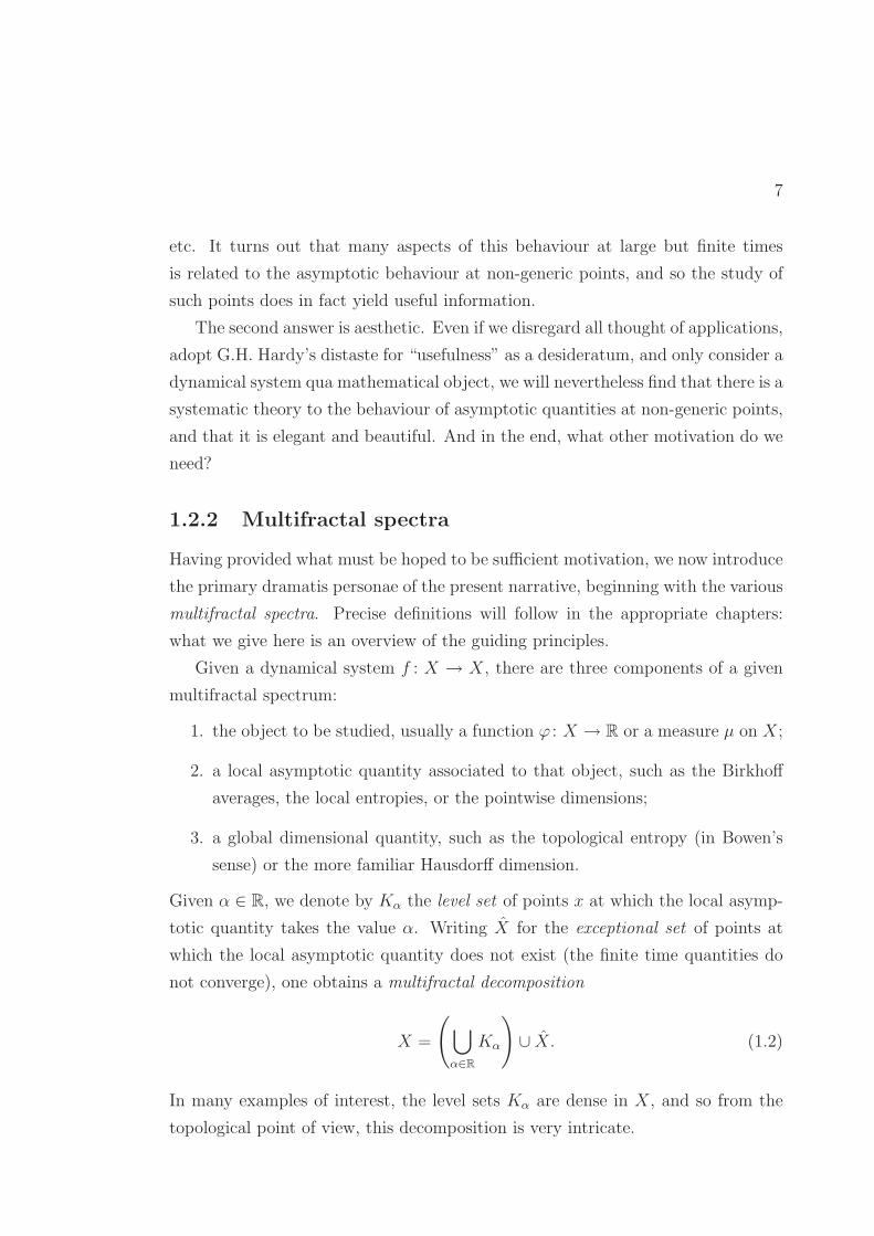
Given α ∈ R, we denote by Kα the level set of points x at which the local asymp-
totic quantity takes the value α. Writing X for the exceptional set of points at
which the local asymptotic quantity does not exist (the finite time quantities do
not converge), one obtains a multifractal decomposition
X =
(
⋃
α∈R
Kα
)
∪ X. (1.2)
In many examples of interest, the level sets Kα are dense in X, and so from the
topological point of view, this decomposition is very intricate.

8
From the measure-theoretic point of view, on the other hand, this decomposi-
tion is very simple. For the Birkhoff averages and the local entropies, the various
ergodic theorems cited above imply that every ergodic measure is supported on
a single level set. The analogous result for pointwise dimensions of hyperbolic
measures was proved by Barreira, Pesin, and Schmeling [BPS99].
From the dimensional point of view, this decomposition is surprisingly inter-
esting. We define the dimension spectrum and the entropy spectrum for the local
quantity in question by
SD(α) = dimH(Kα), SE(α) = htop (Kα). (1.3)
Here htop (Kα) denotes topological entropy in Bowen’s sense: because the level sets
Kα are dense in many natural situations, box dimension and capacity entropy are
of little use in analysing them, as these quantities assign the same value to a set
and to its closure.
After the circuitous manner in which these multifractal spectra are defined—
as dimensions of level sets of asymptotic local quantities—nothing suggests that
their dependence on α should be anything but pathological. Nevertheless, here we
encounter one of the great surprises of the theory, the so-called multifractal miracle:
for a broad class of systems, the multifractal spectra are analytic functions of α!
Moreover, they are concave and can be obtained as the Legendre transform of
convex functions defined at the global level.
This is the central mystery of the subject, and the primary goals of the present
work are to elucidate this phenomenon and investigate the generality in which it
occurs.
1.3 Overview of results
1.3.1 The key tool: thermodynamic formalism
Direct computation of the various multifractal spectra, numerical or otherwise, is
quite difficult. In the first place, in order to determine the level sets Kα explicitly,
one needs to first compute the local asymptotic quantity at every point of X, which
means that ergodic theorems cannot be used. Even if this is accomplished, it still

9
remains to compute the (Bowen) topological entropy or Hausdorff dimension of
Kα for every value of α. Because this quantity is a Caratheodory dimension, and
hence relies on the computation of a critical point, rather than a growth rate, it
is more difficult to compute than the (capacity) topological entropy or the box
dimension.
The failure of the direct frontal assault leads us to introduce our second set
of protagonists, the convex functions mentioned in the previous section, which
sometimes also bear the name of multifractal spectra, but are of a different nature
altogether. The spectra SD(α) and SE(α) are defined in terms of a one-parameter
family of setsKα and a fixed dimensional quantity that measures them. In contrast,
these convex functions are defined in terms of a fixed set—the entire phase space
X—and a one-parameter family of dimensional quantities T (q).
Included in this list are the Henschel–Procaccia spectrum, the Renyi spectrum,
and the correlation entropies, but the most important for our purposes will be the
topological pressure and various thermodynamic functions derived from it.
The topological pressure is the common thread that binds together the dis-
parate actors in our tale, the lynchpin on which the narrative hangs. It may be
thought of as a generalisation of the topological entropy that incorporates informa-
tion regarding the Birkhoff sums of a potential function ϕ. The entropy htop (Z)
is defined in terms of orbit segments of finite length that are distinguishable at a
fixed coarse scale. By counting each such segment with a weight that depends on
the Birkhoff sum of ϕ along the orbit, one obtains the topological pressure PZ(ϕ).
As with the entropy, there are two flavours of pressure: the Caratheodory
pressure, defined as a critical value of a set function, and the capacity pressure,
defined as a growth rate of a certain partition function. On compact invariant sets,
the two pressures agree; furthermore, on such sets they satisfy a crucial variational
principle:
PX(ϕ) = supµ∈Mf (X)
(
h(µ) +
∫
ϕdµ
)
. (1.4)
Here the supremum is over all f -invariant probability measures, and h(µ) is the
measure-theoretic entropy. A measure µ that achieves the supremum in (1.4) is
called an equilibrium state.
As the topological pressure will appear time and time again in various incarna-

10
tions to fill various roles, we take a moment to list a few of its guises here. Because
of the central role the pressure plays, this amounts to giving a capsule summary
of everything that will come in the rest of the story.
1. If a potential ϕ is fixed, the set function Z 7→ PZ(ϕ) is a dimensional quantity
that characterises subsets of X. Conversely, if the set Z is fixed and ϕ is
allowed to vary, the pressure defines a convex function C(X) → R, where
C(X) is the space of all continuous potential functions on X.
2. If Z = X and ϕ varies, then (1.4) may be interpreted in terms of the Leg-
endre transform, a standard tool in thermodynamics. The pressure function
PX : C(X) → R is shown by the variational principle to be the Legendre
transform of the entropy function h : Mf (X) → [0,∞). In Chapter 2, we
will see that under certain conditions, the converse is also true: entropy is
the Legendre transform of pressure. This well-known duality lies at the heart
of our approach to multifractal analysis.
3. If we restrict our attention to the one-dimensional subspace of C(X) spanned
by a fixed potential ϕ, then we obtain a function T : R → R given by T (q) =
PX(qϕ). In Chapter 3, we will see that the equilibrium states νq for the
potentials qϕ can be used to characterise the entropy spectrum for Birkhoff
averages by establishing a function q 7→ α(q) such that νq(Kα(q)) = 1 and
htop (Kα(q)) = h(νq).
4. If we restrict our attention to this subspace and also fix a subset Z ⊂ X,
then we obtain Bowen’s equation PZ(qϕ) = 0. For a broad class of potentials
ϕ, the root of this equation is equal to a dimensional quantity introduced
by Barreira and Schmeling [BS00], denoted dimϕ(Z). In Chapter 4, we will
see that if f is conformal and ϕ is the geometric potential, then dimϕ(Z) is
nothing else but the Hausdorff dimension.
5. One can also consider level sets Kα on which the ratio of the Birkhoff sums
of two functions ϕ and ψ converges to α. In this case, we will see in Chap-
ter 5 that if we implicitly define a function T by PX(qϕ + T (q)ψ) = 0, then
the equilibrium states νq for the potentials qϕ+ T (q)ψ are supported on the

11
level sets Kα(q) for some function q 7→ α(q). Using the results from Chap-
ter 4, we will show that if ψ is the geometric potential for a conformal map
f and µ is a Gibbs measure for ϕ—a measure for which the local entropies
are determined by the Birkhoff averages of ϕ—then this allows us to charac-
terise the dimension spectrum for pointwise dimensions of µ by showing that
dimH(Kα(q)) = dimH(νq).
1.3.2 Deriving multifractal results from thermodynamics
1.3.2.1 The Birkhoff spectrum
Given a compact metric space X, a continuous map f : X → X, and a (Borel)
measurable function ϕ : X → R, the level sets for Birkhoff averages are
KBα = KB
α (ϕ) =
{
x ∈ X∣
∣
∣lim
n→∞
1
nSnϕ(x) = α
}
, (1.5)
where Snϕ(x) =∑n−1
k=0 ϕ(fk(x)) is the nth Birkhoff sum. The entropy spectrum
for Birkhoff averages, which we will simply refer to as the Birkhoff spectrum, is
B(α) = htop (KBα ), (1.6)
where we reiterate that htop is topological entropy in the sense of Bowen. Chapter 3
gives results for the multifractal analysis of the Birkhoff spectrum: these comprise
the first half of the results in [Cli10b].
The strongest result is Theorem 3.1.1, which applies to bounded Borel func-
tions ϕ : X → R for which the closure of the set of discontinuities is given zero
weight by every invariant measure; we denote this class of functions by Af . (Note
that C(X) ⊂ Af .) For such maps and functions, we show that the function
TB : q 7→ PX(qϕ) is the Legendre transform of B(α), without any further re-
strictions on f and ϕ. Furthermore, we show that B(α) is the Legendre trans-
form of TB, completing the multifractal formalism, provided TB is continuously
differentiable and equilibrium measures exist . If the hypotheses on TB only
hold for certain values of q, we still obtain a partial result on B(α) for the corre-
sponding values of α.

12
As stated, Theorem 3.1.1 does not deal with phase transitions—that is, points
at which the pressure function is non-differentiable. Such points correspond (via
the Legendre transform) to intervals over which the Birkhoff spectrum is affine
(if the multifractal formalism holds). In Theorem 3.1.3, we give slightly stronger
conditions on the map f , which are still fundamentally thermodynamic in nature,
under which we can establish the complete multifractal formalism even in the
presence of phase transitions.
It is often the case that thermodynamic considerations demonstrate the exis-
tence of a unique equilibrium state for certain potentials. In Proposition 3.2.1,
we show that if the entropy function is upper semi-continuous, then uniqueness of
the equilibrium state implies differentiability of the pressure function and allows
us to apply Theorem 3.1.1. However, Example 3.1.2 shows that there are systems
for which the pressure function is differentiable, and hence Theorem 3.1.1 can be
applied, even though the equilibrium state is non-unique.
One would like to understand for which classes of discontinuous potentials
the multifractal formalism holds. Things work well for potentials in Af because
the weak* topology is the same at any f -invariant measure whether we consider
continuous test functions or test functions in Af .
If there are invariant measures that give positive weight to the closure of the set
of discontinuities of ϕ, then things are more delicate. One needs to establish con-
ditions under which the invariant measures in which we are particularly interested
still give zero weight to this set. This is achieved by comparing the topological
entropy of this set with the Legendre transform of TB, which allows us to obtain in
Theorem 3.1.4 partial results for any measurable potential that is bounded above
and below.
Ideally, we would be able to include unbounded potentials in these results. In
particular, we would like to be able to consider the geometric potential ϕ(x) =
− log |f ′(x)| for a multimodal map f ; the presence of critical points leads to singu-
larities of ϕ, and so ϕ is not bounded above. Theorem 3.1.5 shows that the results
of Theorem 3.1.1 still hold for q ≤ 0 (that is, values of q such that qϕ is bounded
above) and for the corresponding values of α. The question of what happens for
q > 0 is more delicate and remains open.

13
1.3.2.2 Bowen’s equation
In order to use the techniques of thermodynamic formalism and equilibrium states
to examine the Hausdorff dimensions of level sets in a given multifractal decom-
position, we need a way of determining Hausdorff dimension using topological
pressure. Chapter 4 gives the key result for our purposes, a version of Bowen’s
equation that appeared in [Cli10a] and is given here as Theorem 4.2.1.
The result is given in the setting where X is a compact metric space and
f : X → X is a conformal map. Write f ′(x) for the conformal derivative of f—
that is, the factor by which f expands or contracts nearby points around x. The
precise definition is given in (4.4); two important cases of the definition are when
X is an interval, in which case f ′(x) is the absolute value of the usual derivative,
and when X is a Riemannian manifold, in which case f ′(x) is the positive real
number such that Df(x)/f ′(x) is an isometry.
In this setting, Theorem 4.2.1 shows that for any Z ⊂ X, dimH Z is the smallest
value of t satisfying PZ(−t log(f ′)) = 0, provided the following conditions are met:
1. f has no critical points (f ′(x) = 0) or singularities (f ′(x) = ∞) in X;
2. every point x ∈ Z has positive lower Lyapunov exponent ((fn)′(x) grows
exponentially in n);
3. every point x ∈ Z satisfies a tempered contraction condition.
Note that the first condition must hold on all of X, while the latter two only need
to hold at points in Z.
One can develop the multifractal formalism for Lyapunov exponents; here the
level sets are
KLα =
{
x ∈ X∣
∣
∣lim
n→∞
1
nlog(fn)′(x) = α
}
. (1.7)
It is shown in Theorem 4.2.1 that PKLα
(−t log(f ′)) = htop (KLα ) − tα, and hence
dimH(KLα ) =
htop (KLα )
α. (1.8)
(Note the similarity to (1.1).)
The Lyapunov exponent of a point x is nothing but the Birkhoff average of
log(f ′) at x, and so KLα = KB
α (log(f ′)). Then the entropy spectrum for Lyapunov

14
exponents LE(α) is given as a special case of Theorem 3.1.1, and the form of the
dimension spectrum for Lyapunov exponents LD(α) follows from (1.8).
1.3.2.3 Entropy and dimension spectra of Gibbs measures
There are two other multifractal spectra that are commonly studied: the entropy
spectrum for local entropies, and the dimension spectrum for pointwise dimensions.
Where there is no risk of confusion, we will refer to these as simply as the entropy
spectrum and the dimension spectrum, respectively. We discuss them in Chapter 5,
where we give results on their multifractal analysis that comprise the second half
of the results from [Cli10b].
Both these spectra are characteristics of a fixed measure µ. The level sets for
local entropies hµ(x) and for pointwise dimensions dµ(x) are
KEα = {x ∈ X | hµ(x) = α},
KDα = {x ∈ X | dµ(x) = α}.
The entropy spectrum is given by E(α) = htop (KEα), and the dimension spectrum
by D(α) = dimH(KDα ).
In order to obtain results on these spectra, we need some way to obtain effective
estimates on the small-scale features of µ. In particular, computing hµ(x) requires
estimates on µ(Bn(x)), where Bn(x) is either an n-cylinder or a Bowen ball, and
computing dµ(x) requires estimates on µ(B(x, r)) for small values of r.
These estimates are given by the assumption that µ is a weak Gibbs measure
for a potential function ϕ, which means that the value of hµ(x) is determined
by the Birkhoff average of ϕ along the orbit of x. Consequently, the level sets
KEα are determined by the level sets KB
α (ϕ), and Theorem 3.1.1 for the Birkhoff
spectrum translates directly into Theorem 5.2.1 for the entropy spectrum. Writing
ϕ1 = ϕ− PX(ϕ), we find E(α) as the Legendre transform of the function TE : q 7→
PX(−qϕ1), provided TE is continuously differentiable and equilibrium
measures exist .
So far, the three multifractal spectra considered—for Birkhoff averages, Lya-
punov exponents, and local entropies—all boiled down to the same result concern-
ing level sets of Birkhoff averages. The final spectrum we consider, the dimension

15
spectrum, is a different sort of beast. Suppose that µ is a Gibbs measure for ϕ
and that f is a conformal map for which we write ψ(x) = log f ′(x). Then it can
be shown (in the spirit of (1.1)) that
dµ(x) = limn→∞
−(ϕ(x) + ϕ(f(x)) + · · · + ϕ(fn(x)))
ψ(x) + ψ(f(x)) + · · · + ψ(fn(x)),
and so we are not studying the convergence of a single sequence of Birkhoff sums,
but the convergence of the ratio of two such sequences.
In this case, the proper way to define a thermodynamic function T (q) that is
related to D(α) by the Legendre transform is not to simply work with the one-
dimensional subspace of C(X) spanned by the single potential in question, but
to work with the two-dimensional subspace spanned by ϕ and ψ. In particular,
following Pesin and Weiss [PW97], one passes to ϕ1 so that PX(ϕ1) = 0 and then
defines TD(q) for every q ∈ R as the smallest value of t such that
PX(qϕ1 − tψ) = 0.
Theorem 5.2.2 shows that if f is conformal without critical points or singulari-
ties and if X satisfies the tempered contraction condition mentioned before, then
the implicitly defined function TD(q) is the Legendre transform of the dimension
spectrum D(α), without any further conditions on f or ϕ. Furthermore,
we show that D(α) is the Legendre transform of TD(q), completing the multifrac-
tal formalism, provided TD is continuously differentiable and equilibrium
measures exist .
1.3.3 Relationship with other results
The key ingredients of the multifractal formalism were introduced in [HJK+86],
and the use of the topological pressure as the crucial tool in the analysis goes
back to [Ran89]. Since then, the multifractal spectra for many classes of systems,
potentials, and measures have been studied. The most complete application of
the theory has been to Gibbs measures for Holder continuous potentials on uni-
formly hyperbolic systems, using thermodynamic results due to Bowen [Bow75] on
existence and uniqueness of equilibrium states.

16
Other classes of systems have also been studied, typically on a case-by-case ba-
sis, following the general principle of obtaining multifractal results from knowledge
of the thermodynamics of the system. To date, the general strategy informed by
this philosophy has been as follows:
(1) Fix a specific class of systems—uniformly hyperbolic maps, conformal repellers,
parabolic rational maps, Manneville–Pomeau maps, multimodal interval maps,
etc.
(2) Using tools specific to that class of systems (Markov partitions, specification,
inducing schemes), establish thermodynamic results—existence and unique-
ness of equilibrium states, differentiability of the pressure function, etc.
(3) Using these thermodynamic results together with the original toolkit, study the
multifractal spectra, and show that they can be given in terms of the Legendre
transform of various pressure functions.
The principal novelty of the results presented in this work is to establish the
multifractal formalism for a very general class of systems (including, but not limited
to, most known examples) as a direct corollary of the thermodynamic formalism,
rendering Step (3) above automatic, and eliminating the need for the use of a
specific toolkit to study the multifractal formalism itself. Where these results
duplicate known results, the proofs here are in some cases more direct than the
original proofs.
We will mention previously known results for specific classes of systems in
the later chapters, when we state the theorems that relate to them. For now, we
observe that the only other results that address multifractal formalism for arbitrary
topological dynamical systems are those recently announced by Feng and Huang
in [FH10], which deal with asymptotically sub-additive sequences of potentials,
and which imply Theorem 3.1.1 for continuous potentials ϕ as a special case.
However, their results do not apply to the broader class of bounded measurable
potentials for which we obtain partial results in Theorems 3.1.1 and 3.1.4, nor do
they consider the dimension spectrum. To the best of the author’s knowledge, the
present results are the first rigorous multifractal results for general discontinuous
potentials and for the dimension spectrum of weak Gibbs measures on arbitrary
conformal systems.

Chapter 2Dimension theory and
thermodynamic formalism
2.1 Definitions
2.1.1 Dimensions of sets
In this chapter, we recall the definitions of Hausdorff and box dimension, topolog-
ical entropy, and topological pressure in the general framework of Caratheodory
dimension characteristics introduced by Pesin in [Pes98]. We begin with the Haus-
dorff and box dimensions, which are defined without reference to any underlying
dynamics, before moving on to the definitions at the heart of the thermodynamic
formalism.
Definition 2.1.1. Let X be a separable metric space. Given Z ⊂ X and ε > 0,
let D(Z, ε) denote the collection of countable open covers {Ui}∞i=1 of Z for which
diamUi ≤ ε for all i. For each s ≥ 0, consider the set functions
mH(Z, s, ε) = infD(Z,ε)
∑
Ui
(diamUi)s, (2.1)
mH(Z, s) = limε→0
mH(Z, s, ε). (2.2)

18
The Hausdorff dimension of Z is
dimH Z = inf{s > 0 | mH(Z, s) = 0} = sup{s > 0 | mH(Z, s) = ∞}.
It is straightforward to show that mH(Z, s) = ∞ for all s < dimH Z, and that
mH(Z, s) = 0 for all s > dimH Z.
One may equivalently define Hausdorff dimension using covers by open balls
rather than arbitrary open sets; let Db(Z, ε) denote the collection of countable sets
{(xi, ri)} ⊂ Z × (0, ε] such that Z ⊂⋃
iB(xi, ri), and then define mbH by
mbH(Z, s, ε) = inf
Db(Z,ε)
∑
i
(diamB(xi, ri))s. (2.3)
Finally, define mbH(Z, s) and dimb
H Z by the same procedure as above; then Propo-
sition A.1.1 shows that dimbH Z = dimH Z, so we are free to use either definition.
It is natural to replace (2.3) with
mb′
H(Z, s, ε) = infDb(Z,ε)
∑
i
(2ri)s; (2.4)
however, the two quantities are not necessarily equal, as there are cases in which
diamB(x, r) < 2r (if x is an isolated point, for example, or if X is homeomorphic
to a Cantor set). Nevertheless, Proposition A.1.1 shows that the resulting critical
value dimb′
H Z is equal to dimH Z.
The Hausdorff dimension is the most well-known example of a Caratheodory
dimensional characteristic. If we restrict our attention to covers by balls of a fixed
radius r, the sum in (2.4) takes a particularly simple form, and the critical point
may be computed as a growth rate, giving us the corresponding example of a
capacity dimensional characteristic.
Definition 2.1.2. Given Z ⊂ X and r > 0, let
N(Z, r) = min
{
#Er
∣
∣
∣Er ⊂ Z,
⋃
i
B(xi, r) ⊃ Z
}
be the minimal cardinality of an r-dense set in Z. The lower and upper box di-

19
mensions (or the lower and upper capacity dimensions) of Z are
dimBZ = limr→0
logN(Z, r)
log(1/r), dimBZ = lim
r→0
logN(Z, r)
log(1/r).
In the case Z = X, replacing metric balls B(x, r) by Bowen balls B(x, n, δ)
in this definition yields one of the classical definitions of topological entropy. For
arbitrary subsets Z ⊂ X, we will refer to this as the capacity entropy.
Definition 2.1.3. Let X be a compact metric space and fix a map f : X → X.
The Bowen ball of radius δ and order n is
B(x, n, δ) = {y ∈ X | d(fk(y), fk(x)) < δ for all 0 ≤ k ≤ n}.
A set E ⊂ Z is (n, δ)-spanning if Z ⊂⋃
x∈E B(x, n, δ). Let Qδn be the cardinality of
a minimal (n, δ)-spanning set—one for which no proper subset is (n, δ)-spanning—
and define the lower and upper capacity topological entropies by
Chtop(Z, δ) = limn→∞
1
nlogQδ
n, Chtop(Z, δ) = limn→∞
1
nlogQδ
n, (2.5)
Chtop(Z) = limδ→0
Chtop(Z, δ), Chtop(Z) = limδ→0
Chtop(Z, δ). (2.6)
Elementary arguments given in [Wal75] show that we obtain the same values
for the capacity entropies if we take Qδn to be the cardinality of a maximal (n, δ)-
separated set—that is, a set F ⊂ Z such that B(x, n, δ/2) ∩ B(y, n, δ/2) = ∅ for
all x 6= y ∈ F . We will occasionally have reason to use this definition as well.
The capacity entropies are a direct analogue of the capacity dimensions, ob-
tained by replacing B(x, r) with B(x, n, δ). The same procedure may be carried
out with Hausdorff dimension: this was first done by Bowen [Bow73], who defined
what we will call the Caratheodory topological entropy.
Definition 2.1.4. Given Z ⊂ X, δ > 0, and N ∈ N, let P(Z,N, δ) denote the
collection of countable sets {(xi, ni)}∞i=1 ⊂ Z ×N such that {B(xi, ni, δ)} covers Z

20
and ni ≥ N for all i. For each s ∈ R, consider the set functions
mh(Z, s,N, δ) = infP(Z,N,δ)
∑
(xi,ni)
e−nis, (2.7)
mh(Z, s, δ) = limN→∞
mh(Z, s,N, δ), (2.8)
and put
htop (Z, δ) = inf{s > 0 | mh(Z, s, δ) = 0} = sup{s > 0 | mh(Z, s, δ) = ∞}.
As with Hausdorff dimension, we get mh(Z) = ∞ for s < htop (Z, δ), and mh(Z) =
0 for s > htop (Z, δ). The topological entropy of f on Z is
htop (Z) = limδ→0
htop (Z, δ).
Given a potential function ϕ : X → R, the classical topological entropy gen-
eralises to the topological pressure by giving each element in a minimal (n, δ)-
spanning set a weight that depends on the nth Birkhoff sum of the potential ϕ at
x. Once again, carrying out this procedure for an arbitrary subset Z ⊂ X yields
the capacity topological pressure.
Definition 2.1.5. Given a potential ϕ, we denote the Birkhoff sums by
Snϕ(x) = ϕ(x) + ϕ(f(x)) + · · · + ϕ(fn−1(x)).
Fix a subset Z ⊂ X. For every n ∈ N, δ > 0, let Eδn be a minimal (n, δ)-spanning
set and define a partition function Rδn(ϕ) by
Rδn(ϕ) =
∑
x∈Eδn
eSnϕ(x).
Then the lower and upper capacity topological pressures of ϕ on Z are given by
CPZ(ϕ, δ) = limn→∞
1
nlogRδ
n(ϕ), CPZ(ϕ, δ) = limn→∞
1
nlogRδ
n(ϕ), (2.9)
CPZ(ϕ) = limδ→0
CPZ(ϕ, δ), CPZ(ϕ) = limδ→0
CPZ(ϕ, δ). (2.10)

21
In the case ϕ = 0, these reduce to Chtop(Z) and Chtop(Z), respectively.
By including a factor of eSni(xi) for each element of a cover by Bowen balls, a
similar modification may be made to the definition of Caratheodory entropy; this
was introduced by Pesin and Pitskel’ in [PP84].
Definition 2.1.6. Given a potential function ϕ and a subset Z ⊂ X, consider the
following set functions for every δ > 0 and N ∈ N:
mP (Z, s, ϕ,N, δ) = infP(Z,N,δ)
∑
(xi,ni)
exp (−nis+ Sniϕ(xi)) ,
mP (Z, s, ϕ, δ) = limN→∞
mP (Z, s, ϕ,N, δ).
(2.11)
The latter function is non-increasing in s, and takes values ∞ and 0 at all but at
most one value of s. Denoting the critical value of s by
PZ(ϕ, δ) = inf{s ∈ R | mP (Z, s, ϕ, δ) = 0} = sup{s ∈ R | mP (Z, s, ϕ, δ) = ∞},
we get mP (Z, s, ϕ, δ) = ∞ when s < PZ(ϕ, δ), and 0 when s > PZ(ϕ, δ).
The Caratheodory topological pressure of ϕ on Z is PZ(ϕ) = limδ→0 PZ(ϕ, δ).
Once again, in the case ϕ = 0 this reduces to htop (Z).
Basic properties and results concerning all these definitions are given in the
next section. For now, we remark that the definitions of Caratheodory entropy
and pressure given here differ slightly from the definitions in [Pes98]. Nevertheless,
Proposition A.2.1 shows that they yield the same quantity.
2.1.2 Basic properties
Because the quantities defined in the previous section all fit into the general frame-
work of Caratheodory characteristics, they all satisfy a number of general proper-
ties given in [Pes98]. We will use two of these repeatedly, so they are worth giving
special mention here.

22
In the first place, given any countable family of sets Zi ⊂ X, we have
dimH
(
⋃
i
Zi
)
= supi
dimH Zi,
htop
(
⋃
i
Zi
)
= supi
htop Zi,
P⋃i Zi
(ϕ) = supi
PZi(ϕ).
(2.12)
It is important to note that this property of countable stability (or σ-stability) only
holds for the Caratheodory dimensions, and not for the capacities. Indeed, this is
one of the chief advantages of the Caratheodory dimensions for our purposes.
The second important general property is that the Caratheodory dimensions
are bounded above by the capacities:
dimH Z ≤ dimBZ ≤ dimBZ, (2.13)
htop Z ≤ ChtopZ ≤ ChtopZ, (2.14)
PZ(ϕ) ≤ CPZ(ϕ) ≤ CPZ(ϕ). (2.15)
It is then a question of interest to know when the three quantities coincide. For
Hausdorff dimension and box dimension, there is no completely satisfactory general
theory; for entropy and pressure, on the other hand, it is shown in [Pes98] that
if Z is compact and f -invariant (for example, if Z = X), then we have equality
in (2.14) and (2.15).
2.1.3 Dimensions of measures
Given a separable metric space X, let M(X) denote the set of all Borel probabil-
ity measures on X. The Caratheodory dimensional characteristics defined in the
previous section can be made meaningful for measures µ ∈ M(X) as well.
Definition 2.1.7. Given µ ∈ M(X), the Hausdorff dimension of µ is
dimH(µ) = inf{dimH Z | Z ⊂ X,µ(Z) = 1}.

23
Similarly, the entropy of µ is
h(µ) = inf{htop Z | Z ⊂ X,µ(Z) = 1},
and the pressure of µ with respect to a potential ϕ is
Pµ(ϕ) = inf{PZ(ϕ) | Z ⊂ X,µ(Z) = 1}.
One could also define the above quantities for the corresponding capacities, but
we will not use this fact.
We point out that these definitions are given for arbitrary probability measures
µ, which may not be invariant. We will see shortly that in the case where µ is
invariant and ergodic, then h(µ) is equal to the usual measure-theoretic entropy,
and Pµ(ϕ) = h(µ) +∫
ϕdµ.
In many cases, we can obtain information about these global quantities (and
the corresponding Caratheodory dimensions for sets) by studying a related set of
local quantities.
Definition 2.1.8. Given µ ∈ M(X) and x ∈ X, the lower and upper pointwise
dimensions of µ at x are
dµ(x) = limr→0
log µ(B(x, r))
log r, dµ(x) = lim
r→0
log µ(B(x, r))
log r.
If the two quantities agree, we denote the common value by dµ(x), and call it the
pointwise dimension. Similarly, the lower and upper local entropies are
hµ(x) = limδ→0
limn→∞
−1
nlog µ(B(x, n, δ)), hµ(x) = lim
δ→0lim
n→∞−
1
nlog µ(B(x, n, δ)),
with common value hµ(x) if the limit exists, and the lower and upper local pressures
are
P µ(x) = limδ→0
limn→∞
1
n(− log(µ(B(x, n, δ))) + Snϕ(x)),
P µ(x) = limδ→0
limn→∞
1
n(− log(µ(B(x, n, δ))) + Snϕ(x)).

24
We remark that this last piece of terminology is not standard: the local quantity
introduced in [Pes98] corresponding to pressure is somewhat different, but we will
be able to use this quantity to derive the same sorts of results.
2.1.4 Global information from local quantities
The following result uses easy arguments from [Pes98]; a proof for the case of
pressure is given in Theorem B.1.1 in Appendix B.
Proposition 2.1.1. Let dim denote any of the three Caratheodory dimensions
dimH(·), htop (·), or P·(ϕ), and let µ ∈ M(X) and Z ⊂ X be arbitrary. Then
dimZ ≤ supx∈Z
dimµ(x). (2.16)
Furthermore, if µ(Z) > 0, then
dimZ ≥ infx∈Z
dimµ(x). (2.17)
The following corollary allows us to apply ergodic results to relate h(µ) and
Pµ(ϕ) to familiar quantities.
Corollary 2.1.2. Let dim be as in Proposition 2.1.1 and suppose that for some
measure µ ∈ M(X) we have
dimµ(x) = dimµ(x) = α (2.18)
on a set of full measure (with respect to µ). Then dim(µ) = α.
Proof. We see from (2.17) that dimZ ≥ α for every Z ⊂ X with µ(Z) = 1.
Furthermore, let Z be the set of points on which (2.18) holds: then µ(Z) = 1 and
Proposition 2.1.1 implies that dimZ = α.
Using the Brin–Katok entropy formula and Birkhoff’s ergodic theorem, we see
that if µ is ergodic and invariant, then we have the following for µ-a.e. x:
hµ(x) = hµ(x) = hµ(f),
P µ(x) = P µ(x) = hµ(f) +
∫
ϕdµ.

25
Here hµ(f) is the usual measure-theoretic (Kolmogorov–Sinai) entropy: Corol-
lary 2.1.2 shows that hµ(f) = h(µ), where the latter quantity is the dimensional
quantity defined in the previous section, whenever µ is ergodic and invariant. (If
µ is not ergodic, the two quantities may differ.)
It follows immediately from these remarks and the definition of dimµ that
h(µ) ≤ htop (X) for every ergodic invariant measure µ, and more generally,
h(µ) +
∫
ϕdµ ≤ PX(ϕ). (2.19)
This is one half of the variational principle, which we will explore more in the next
section.
Proposition 2.1.1 and Corollary 2.1.2 show that knowledge of local dimensional
quantities of a measure at almost every point gives us knowledge of global dimen-
sional quantities of that same measure, and hence also gives a lower bound for
the dimensional quantities of a set on which the measure sits. Furthermore, the
proposition shows that if we have knowledge of the local quantity at every point
in the set, then we obtain an upper bound for the dimensional quantity of the set.
In particular, if hµ(x) = h(µ) for every x ∈ X, then h(µ) = htop (X), and so µ is
a measure of maximal entropy. A similar statement holds for Pµ(x), and we will
investigate this in due course.
2.2 Thermodynamic formalism
2.2.1 The variational principle
We now consider a compact metric space X and a continuous map f : X → X.
Once again, let M(X) denote the set of all Borel probability measures on X;
furthermore, let Mf (X) be the set of f -invariant measures in M(X), and let
MfE(X) be the set of all ergodic measures in Mf (X).
Definition 2.2.1. Let ϕ : X → R be measurable and bounded above and below.
Given Z ⊂ X, the (variational) pressure of ϕ on Z is
P ∗Z(ϕ) = sup
{
h(µ) +
∫
ϕdµ∣
∣
∣µ ∈ Mf (X), µ(Z) = 1
}
. (2.20)

26
A measure ν ∈ Mf (X) is an equilibrium state for the potential ϕ if it achieves this
supremum; that is, if
P ∗(ϕ) = h(ν) +
∫
ϕdν.
Every equilibrium state is a convex combination of ergodic equilibrium states, and
it follows using the ergodic decomposition that (2.20) is equivalent to
P ∗Z(ϕ) = sup
{
h(µ) +
∫
ϕdµ∣
∣
∣µ ∈ Mf
E(X), µ(Z) = 1
}
.
The following well-known result lies at the very heart of the thermodynamic
formalism. We do not give a complete proof here, but mention the key ideas of an
approach due to Misiurewicz.
Theorem 2.2.1 (Variational Principle). Let X be a compact metric space, f : X →
X a continuous map, and ϕ : X → R a continuous potential. Then P ∗(ϕ) =
PX(ϕ).
Proof. It follows from (2.19) that P ∗(ϕ) ≤ PX(ϕ), and so it remains only to
construct a family of invariant measures µ for which Pµ(ϕ) = h(µ) +∫
ϕdµ is
arbitrarily close to PX(ϕ). This is done as follows, using the fact that PX(ϕ) =
CPX(ϕ) = CPX(ϕ) since X is compact and invariant.
Let δ > 0 be arbitrary, and let En ⊂ X be a maximal (n, δ)-separated set.
Define an atomic measure σn on En by
σn =
∑
y∈EneSnϕ(y)δy
∑
z∈EneSnϕ(z)
, (2.21)
and define µn by
µn =1
n
n−1∑
i=0
σn ◦ f−i. (2.22)
Let µ be any weak* limit of the sequence µn—then µ is invariant, and it is shown
in the proof of [Wal75, Theorem 9.10] that
h(µ) +
∫
ϕdµ ≥ CPX(ϕ, δ). (2.23)
Letting δ go to 0 gives the result.

27
2.2.2 Pressure, entropy, and the Legendre transform
We now introduce a key mathematical tool that is commonly used in thermody-
namics (although the version used here differs slightly).
Definition 2.2.2. Let V be a topological vector space, and let V ∗ be the dual
space comprising all continuous linear functionals v∗ : V → R. Given a function
T : V → R ∪ {+∞} (which we will usually take to be convex), the Legendre
transform of T is the function TL1 : V ∗ → R ∪ {−∞} given by
TL1(v∗) = infv∈V
(T (v) − v∗(v)). (2.24)
Conversely, given a function S : V ∗ → R∪{−∞} (which we will usually take to be
concave), the Legendre transform of S is the function SL2 : V → R ∪ {+∞} given
by
SL2(v) = supv∗∈V ∗
(S(v∗) + v∗(v)). (2.25)
Figure 3.1 shows two functions that are related by a Legendre transform.
Recall that a function S : V ∗ → R is concave if
S(tv∗ + (1 − t)w∗) ≥ tS(v∗) + (1 − t)S(w∗)
for every v∗, w∗ ∈ V ∗ and t ∈ [0, 1], and S is upper semi-continuous if
S(v∗) ≥ limw∗→v∗
S(w∗)
for every v∗ ∈ V ∗. It is easy to show that the infimum of a family of concave and
upper semi-continuous functions is itself concave and upper semi-continuous. In
particular, for every v ∈ V , the function v∗ 7→ T (v) − v∗(v) is affine, and hence
concave and upper semi-continuous; it follows that TL1 : V ∗ → R is concave and
upper semi-continuous, no matter what T is. Similarly, SL2 : V → R is auto-
matically convex and lower semi-continuous (that is, the above inequalities are
reversed).
In fact, one may show that (SL2)L1 is the concave and upper semi-continuous
hull of S—that is, the infimum of all concave and upper semi-continuous func-

28
tions greater than or equal to S—and that (TL1)L2 is the convex and lower semi-
continuous hull of T .
Remark. The standard definition of the Legendre–Fenchel transform in thermo-
dynamics differs from (2.24) by a sign, being given by TL(v∗) = supv∈V (v∗(v) −
T (v)) = −TL1(v∗). This takes convex functions to convex functions, rather than to
concave functions, as does our definition, and acts as its own inverse on the space
of convex functions. The difference in the present definition is due to the fact
that we wish to deal with some functions that are naturally convex (topological
pressure) and some that are naturally concave (measure-theoretic entropy).
We can use the language of Legendre transforms to gain further insight into the
relationship between topological pressure and measure-theoretic entropy. Indeed,
setting V = C(X) so that V ∗ = C(X)∗ ⊃ Mf (X), we see that the variational
pressure function ϕ 7→ P ∗X(ϕ) is nothing but the Legendre transform of the entropy
function µ 7→ hµ(f). Thus by the variational principle, the topological pressure
function ϕ 7→ PX(ϕ) is given by this same Legendre transform.
What we would like to do, though, is to understand the space of invariant
measures in terms of the pressure function, not the other way round. By the
above remarks, the Legendre transform of the pressure function is the upper semi-
continuous hull of the entropy function (which is already concave, even affine).
Thus we have the following result: if the entropy function is upper semi-continuous,
then it is completely determined by the pressure function.
The entropy function is an infinite-dimensional beast, being defined on a Cho-
quet simplex whose set of extreme points is the collection of all ergodic invariant
measures. The principle guiding our multifractal results in Chapters 3 and 5 is that
the various multifractal spectra are in some sense one-dimensional projections of
this infinite-dimensional entropy function, and that the aforementioned result on
the Legendre transform can be applied to them as well by finding the appropriate
families of equilibrium states.

Chapter 3Multifractal analysis of Birkhoff
averages
3.1 Main results
3.1.1 Nearly continuous potentials, differentiable pressure
In this chapter, we state our main results for the Birkhoff spectrum defined in (1.5)
and (1.6). Our goal is to obtain B(α) as the Legendre transform of the function
TB(q) = PX(qϕ) = P ∗(qϕ); because we are dealing now with functions of a single
variable, rather than functions defined on some larger topological vector space, the
(convex to concave) Legendre transform (2.24) takes the form
TL1(α) = infq∈R
(T (q) − qα), (3.1)
where T : R → R ∪ {+∞} is any function, which in our case will be the convex
function TB. Similarly, the (concave to convex) Legendre transform of S : R →
R ∪ {−∞} defined in (2.25) is given here by
SL2(q) = supα∈R
(S(α) + qα). (3.2)
In what follows, we will consider situations in which the function T is given
in terms of the pressure function, and is known to be convex and lower semi-

30
continuous (usually even continuous), but the function S is one of the multifractal
spectra, about which we have no a priori knowledge. Thus while (TL1)L2 will be
automatically equal to T , all we can say in general is that (SL2)L1 is the concave and
upper semi-continuous hull of S (note that concavity implies upper semi-continuity
except possibly at points on the boundary of S−1(−∞)).
If S(x) ≥ 0 for every x ∈ R, then SL2 is infinite everywhere. Thus for pur-
poses of defining the various multifractal spectra, we adopt the (non-standard)
convention that htop (∅) = dimH(∅) = −∞.
We recall that if T is known to be convex, then left and right derivatives exist
at every point that has a neighbourhood on which T is finite; we will denote these
by
D−T (q) = limq′→q−
T (q) − T (q′)
q − q′, D+T (q) = lim
q′→q+
T (q′) − T (q)
q′ − q.
Existence follows from monotonicity of the slopes of the secant lines. Given a
convex function T , define a map from R to closed intervals in R by A(q) =
[D−T (q), D+T (q)]. Extend this in the natural way to a map from subsets of R
to subsets of R; we will again denote this map by A. This map has the following
useful property: given any set IQ ⊂ R and α ∈ A(IQ), we have
TL1(α) = infq∈IQ
(T (α) − qα).
This will be important for us in settings where we only have partial information
about the functions T and S. We will also make use of a map in the other direction:
given a set IA ⊂ R (in the domain of S), we denote the set of corresponding values
of q by
Q(IA) = {q ∈ R | A(q) ∩ IA 6= ∅}.
In particular, if α = T ′(q), then α = A(q), and if q = −S ′(α), then q = Q(α). If
(q1, q2) is an interval on which T is affine, then A((q1, q2)) is the slope of T on that
interval; furthermore, TL1 has a point of non-differentiability at A((q1, q2)).
In the results below, it will sometimes be important to know whether or not T
is differentiable. A standard cardinality argument shows that D−T (q) = D+T (q)
at all but countably many values of q; however, the values of q at which differen-
tiability fails may a priori be dense in R.

31
Before stating our most general result, we describe the class of functions to
which it applies. Given a function ϕ : X → R, let C(ϕ) ⊂ X denote the set of
points at which ϕ is discontinuous. Then we let Af denote the class of Borel
measurable functions ϕ : X → R which satisfy the following conditions:
(A) ϕ is bounded (both above and below);
(B) µ(C(ϕ)) = 0 for all µ ∈ Mf (X).
In particular, Af includes all continuous functions ϕ ∈ C(X,R). It also includes all
bounded measurable functions ϕ for which C(ϕ) is finite and contains no periodic
points, and more generally, all bounded measurable functions for which C(ϕ) is
disjoint from all its iterates.
We will see later (Proposition 3.3.1) that passing from C(X,R) to Af does not
change the weak* topology at measures in Mf (X), which is the key to including
these particular discontinuous functions in our results.
Theorem 3.1.1 (The entropy spectrum for Birkhoff averages). Let X be a compact
metric space, f : X → X be continuous, and ϕ ∈ Af . Then
I. TB is the Legendre transform of the Birkhoff spectrum:
TB(q) = BL2(q) = supα∈R
(B(α) + qα) (3.3)
for every q ∈ R.
II. The set {α ∈ R | B(α) > −∞} is bounded by the following:
αmin = inf{α ∈ R | TB(q) ≥ qα for all q}, (3.4)
αmax = sup{α ∈ R | TB(q) ≥ qα for all q}, (3.5)
That is, KBα = ∅ for every α < αmin and every α > αmax.
III. Suppose that TB is Cr on (q1, q2) for some r ≥ 1, and that for each q ∈ (q1, q2),
there exists a (not necessarily unique) equilibrium state νq for the potential
function qϕ. Let α1 = D+TB(q1) and α2 = D−TB(q2); then
B(α) = TL1B (α) = inf
q∈R
(TB(q) − qα) (3.6)

32
TB(q)
q
B(α)
α
Figure 3.1. The Birkhoff spectrum for a map with no phase transitions.
for all α ∈ (α1, α2). In particular, B(α) is strictly concave on (α1, α2), and
Cr except at points corresponding to intervals on which TB is affine.
Observe that the first two statements hold for every continuous map f , without
any assumptions on the system, thermodynamic or otherwise. For discontinuous
potentials in Af , these are the first rigorous multifractal results of any sort known
to the author.
Using the maps A and Q introduced above, Part III can be stated as follows:
if TB is Cr on an open interval IQ and equilibrium states exist for all q ∈ IQ,
then (3.6) holds for all α ∈ A(IQ). If in addition TB is strictly convex on IQ, then
B(α) is Cr on A(IQ).
We will show later that if the entropy map is upper semi-continuous, then
the conclusion of Part III holds at α1 and α2 as well. We will also see (Propo-
sition 3.2.1) that existence of a unique equilibrium state on an interval (q1, q2) is
enough to guarantee differentiability, and hence to apply Theorem 3.1.1. As shown
in Example 3.1.2 below, though, we may have differentiability without uniqueness.
3.1.2 Phase transitions, non-differentiable pressure
If TB is continuously differentiable for all q, then Theorem 3.1.1 gives the com-
plete Birkhoff spectrum, as shown in Figure 3.1. However, there are many phys-
ically interesting systems which display phase transitions—that is, values of q at
which TB is non-differentiable. For example, if f : [0, 1] → [0, 1] is the Manneville–
Pomeau map and ϕ is the geometric potential log |f ′|, then TB is as shown in Fig-
ure 3.2 [Nak00]; in particular, TB is not differentiable at q0. Thus Theorem 3.1.1
gives the Birkhoff spectrum on the interval [α1, α2], where α1 = limq→q+0T ′B(q), but
says nothing about the interval [0, α1), on which TL1B (α) = −q0α is linear.

33
TB(q)
qq0
B(α)
αα2α1
Figure 3.2. A phase transition in the Manneville–Pomeau map.
TB(q)
q
X1X2
B(α)
α
X1 X2
TL2B
α1
α2 α3
α4
Figure 3.3. A different sort of phase transition.
In fact, it is known that for this particular example, we have B(α) = TL1B
even on the linear stretch corresponding to the point of non-differentiability of
TB [Nak00]. However, this is not universally the case, as may be seen by “gluing
together” two unrelated maps. Consider two maps f1 : X1 → X1 and f2 : X2 → X2,
where X1 and X2 are disjoint, and suppose that the thermodynamic functions
are as shown in Figure 3.3. Let X = X1 ∪ X2, and define a map f : X → X
such that the restriction of f to Xi is fi for i = 1, 2. Then TB(q) = P ∗(qϕ) =
max{P ∗1 (qϕ|X1), P
∗2 (qϕ|X2)}, where P ∗
i denotes the pressure of fi, and furthermore
B(α) is the maximum of htop (KBα ∩ X1) and htop (KB
α ∩ X2). Thus TB is non-
differentiable at q = 0, which corresponds to the interval [α2, α3] on which TL1B
is constant. Applying Theorem 3.1.1 to each of the subsystems fi, we see that
B(α) = TL1B (α) on [α1, α2] and [α3, α4], but that the two are not equal on (α2, α3),
and that B(α) is not concave on this interval.
Example 3.1.2. Given m,n ∈ N, let (X1, f1) = (Σ+m, σ) and (X2, f2) = (Σ+
n , σ) be
the full one-sided shifts on m and n symbols, respectively, and construct f : X → X
as above, where X = X1 ∪X2. Choose two vectors v ∈ Rm and w ∈ R
n, and let

34
ϕ : X → R be given by
ϕ(x) =
vx1 x = x1x2 · · · ∈ X1 = Σ+m,
wx1 x = x1x2 · · · ∈ X2 = Σ+n .
Then an easy computation using the classical definition of pressure and the varia-
tional principle shows that
TB(q) = P ∗(qϕ) = max(P ∗1 (qϕ), P ∗
2 (qϕ))
= max
(
log
(
m∑
i=1
eqvi
)
, log
(
n∑
j=1
eqwj
))
.
In particular, we see that P ∗1 (0) = logm and P ∗
2 (0) = log n, and also that
dk
dqkP ∗
1 (qϕ)|q=0 = log
(
∑
i
vki
)
,
dk
dqkP ∗
2 (qϕ)|q=0 = log
(
∑
j
wkj
)
.
(3.7)
By judicious choices of v and w, we can observe a variety of behaviours in the
Birkhoff spectrum B(α). If m = n but∑
i vi 6=∑
j wj, we obtain the picture
shown in Figure 3.3.
If m = n and∑
i vi =∑
j wj, but∑
i v2i >
∑
j w2j , then the two pressure
functions P ∗1 (qϕ) and P ∗
2 (qϕ) are tangent at q = 0, corresponding to the existence
of two ergodic measures of maximal entropy (one on X1 and one on X2), but for
values of q near 0, there is a unique equilibrium state supported on X1.
Finally, if m = n and∑
i vki =
∑
j wkj for k = 1, 2, but not for k = 3, then
the two pressure functions are still tangent at q = 0, but now the equilibrium
state passes from X1 to X2 as q passes through 0. Despite this transition and the
non-uniqueness of the measure of maximal entropy, the pressure function TB is still
differentiable at 0.
Remark. The “gluing” in the previous example is introduced quite artificially. How-
ever, a similar phenomenon occurs naturally when one considers renormalisable
maps; these display phase transitions in which the support of the equilibrium state

35
jumps from one compact invariant set to another [Dob09].
Having seen two very different manifestations of phase transitions (Figures 3.2
and 3.3), we see that any generalisation of Theorem 3.1.1 that treats phase tran-
sitions must somehow distinguish between these two sorts of behaviour. The key
difference is that in the first case, the system f : X → X can be approximated from
within by a sequence of subsystems Xn on which there is no phase transition—that
is, the following condition holds [Nak00, GR09]:
(A) There exists a sequence of compact f -invariant subsets Xn ⊂ X such that the
pressure function q 7→ P ∗Xn
(qϕ) is continuously differentiable for all q ∈ R
(and equilibrium states exist), and furthermore,
limn→∞
P ∗Xn
(qϕ) = P ∗(qϕ). (3.8)
This condition fails for the example in Figure 3.3, in which the phase transition rep-
resents a jump from one half of the system to the other half, which is disconnected
from the first, rather than an escaping of measures to an adjacent fixed point. Us-
ing Condition (A), we can state a general theorem which extends Theorem 3.1.1
to maps for which TB has points of non-differentiability.
Theorem 3.1.3. Let X be a compact metric space, f : X → X be continuous, and
ϕ ∈ Af . If Condition (A) holds, then we have (3.6) for all α ∈ (αmin, αmax).
3.1.3 General discontinuous potentials
As mentioned just before Theorem 3.1.1, the key property of potentials ϕ ∈ Af is
that weak* convergence to an invariant measure implies convergence of the integrals
of ϕ; this is the only place in the proof where we use the requirement that ϕ lie in
Af .
For potentials outside of Af , we can try to regain approximate convergence
results at certain relevant measures by using the topological entropy of C(ϕ) to
give a bound on how much weight a neighbourhood of C(ϕ) carries.
To this end, given h ≥ 0, consider the set
IA(h) = {α ∈ R | TL1B (α) > h},

36
and also its counterpart
IQ(h) = Q(IA(h)).
Geometrically, IQ(h) may be described as the set of values q ∈ R such that there
is a line through (q, TB(q)) that lies on or beneath the graph of TB and intersects
the y-axis somewhere above (0, h).
Theorem 3.1.4. Let X be a compact metric space, f : X → X be continuous, and
ϕ : X → R be measurable and bounded (above and below). Let C(ϕ) be the set of
discontinuities of ϕ, and let h0 = Chtop(C(ϕ)). Then
I. For every q ∈ IQ(h0), we have the following version of (3.3):
TB(q) = supα∈IA(h0)
(B(α) + qα). (3.9)
II. B(α) ≤ h0 for every α /∈ IA(h0).
III. Suppose that TB is Cr on (q1, q2) ⊂ IQ(h0) for some r ≥ 1, and that for each
q ∈ (q1, q2) there exists a (not necessarily unique) equilibrium state νq for the
potential function qϕ. Then (3.6) holds for all α ∈ (α1, α2) = A((q1, q2)).
Finally, although we are not yet able to give a complete treatment of unbounded
potential functions, we can show that everything works if our potential function is
bounded below and we only consider q ≤ 0.
Theorem 3.1.5. Let X be a compact metric space, f : X → X be continuous, and
ϕ : X → R ∪ {+∞} be continuous where finite (and hence bounded below). Let
α0 = D−TB(0), and let αmin be given by (3.4), so (αmin, α0) = A((−∞, 0)). Then
I. For every q ≤ 0, (3.3) holds.
II. For α < αmin, we have KBα = ∅.
III. Suppose that TB is Cr on (q1, q2) for some r ≥ 1 and q1 < q2 ≤ 0, and that
for each q ∈ (q1, q2) there exists a (not necessarily unique) equilibrium state
νq for the potential qϕ. Then (3.6) holds for all α ∈ (α1, α2) = A((q1, q2)).
An analogous result holds for q ≥ 0 if ϕ is bounded above but not below. Also,
as with Theorem 3.1.1, Part III extends to the endpoints αi if the entropy map is
upper semi-continuous.

37
3.2 Applications and relation to other results
3.2.1 Verifying the hypotheses
3.2.1.1 Nearly continuous potentials
Parts I and II of Theorem 3.1.1 do not place any thermodynamic requirements
on the function TB, and thus hold in full generality: for every continuous map f
and every potential ϕ ∈ Af , the pressure function TB is the Legendre transform of
B(α) (and hence TL1B is the concave hull of B(α)), and the domain of the Birkhoff
spectrum is the interval [αmin, αmax].
There are two thermodynamic requirements in Part III—existence of an equi-
librium state, and differentiability of TB. The latter is used in order to guarantee
the existence of values q ∈ R for which T ′B(q) exists, and hence A(q) = {T ′
B(q)}
is a singleton. In fact, because T is continuous and convex, A(q) is a singleton
for all but at most countably many values of q, and consequently, once existence
of equilibrium states is established, it follows that the Birkhoff spectrum is equal
to the Legendre transform of the pressure function everywhere except possibly on
some countable union of intervals, on each of which that Legendre transform is
affine and gives an upper bound for B(α).
Existence of equilibrium states is easy to verify in the following rather common
setting.
Definition 3.2.1. The entropy map µ 7→ h(µ) is upper semi-continuous if for
every sequence µn ∈ Mf (X) that converges to µ in the weak* topology, we have
limn→∞
h(µn) ≤ h(µ).
If the entropy map is upper semi-continuous and ϕ is continuous, then the map
µ 7→ h(µ) +
∫
qϕ dµ
is upper semi-continuous for every q ∈ R, and thus attains its maximum, since the
space of invariant measures is compact. In particular, there exists an equilibrium
state for every qϕ.

38
Definition 3.2.2. f is expansive if there exists ε > 0 such that for all x 6= y
there exists n ∈ Z (if f is invertible) or n ∈ N (if f is non-invertible) such that
d(fn(x), fn(y)) ≥ ε.
For expansive homeomorphisms, the entropy map µ 7→ hµ(f) is upper semi-
continuous [Wal75, Theorem 8.2], and so existence is guaranteed for continuous
ϕ. Similarly, the entropy map is upper semi-continuous for C∞ maps of compact
smooth manifolds [New89], and we once again get existence for free.
Proposition 3.2.1. Let X be a compact metric space, f : X → X a continuous
map, and ϕ ∈ Af . Suppose that the entropy map is upper semi-continuous and that
there exists an interval (q1, q2) ⊂ R such that for every q ∈ (q1, q2), the potential
qϕ has a unique equilibrium state. Then TB is C1 on (q1, q2).
Proof. Suppose for a contradiction that the pressure function q 7→ P ∗(qϕ) is not
differentiable at q0 ∈ (q1, q2). Let µ−n be the unique equilibrium state for (q− 1
n)ϕ,
and let µ− be a weak* limit of some subsequence µ−nj
. By upper semi-continuity
and Proposition 3.3.1 below, we have
h(µ−) +
∫
qϕ dµ− ≥ limnj→∞
h(µnj) +
∫
qϕ dµ−nj
= limnj→∞
P ∗
((
q −1
nj
)
ϕ
)
= P ∗(qϕ).
Thus µ− is an equilibrium state for qϕ with
∫
qϕ dµ− = D−TB(q) = limq′→q−
T ′B(q′)
by Proposition 3.4.3 below. Similarly, one can construct an equilibrium state µ+
such that∫
qϕ dµ+ is the right derivative of TB at q. If the two derivatives do not
agree, then we have two distinct equilibrium states for qϕ, a contradiction.
Using Proposition 3.2.1, one approach to verifying the hypotheses of Theo-
rem 3.1.1 for a map with upper semi-continuous entropy is to show that the equi-
librium state for each qϕ is unique.
We also observe that in the context of Part III of Theorem 3.1.1, the construc-
tion in the proof above gives equilibrium states for q1ϕ and q2ϕ that are supported

39
on the sets KBα1
and KBα2
, respectively, and which establish (3.6) for the endpoints
α1 and α2, just as in the proof of Proposition 3.4.2 below.
3.2.1.2 General discontinuous potentials
If ϕ is discontinuous, the map from M(X) to R defined by
µ 7→
∫
ϕdµ (3.10)
is not continuous on all of M(X). For discontinuous potentials lying in Af , conti-
nuity still holds at measures in Mf (X) by Proposition 3.3.1 below, which suffices
for all the proofs here.
However, if ϕ /∈ Af , then there may be invariant measures at which the map is
discontinuous. In particular, if µ(C(ϕ)) > 0, then the map in (3.10) is discontinuous
at µ. If ϕ is unbounded, then it is relatively straightforward to show that the map
is not continuous at any measure in M(X). In many cases, it is not even enough
to restrict our attention to invariant measures [BK98, Proposition 2.8]. Thus for
ϕ /∈ Af , upper semi-continuity of the entropy is not enough to guarantee existence
of equilibrium states without further information.
For potentials which are bounded above but not below, we observe in Propo-
sition 3.3.2 that the map in (3.10) is upper semi-continuous, and thus the free
energy function µ 7→ h(µ) +∫
ϕdµ is upper semi-continuous as well. It follows
that it attains its maximum, and we once again are guaranteed existence. This is
also enough to prove Proposition 3.2.1 for these potentials, showing that existence
and uniqueness imply differentiability of the pressure function (for the appropriate
sign of q) if the entropy map is upper semi-continuous.
3.2.2 The Lyapunov spectrum
An important special case of the Birkhoff spectrum occurs when f is a conformal
map (this is automatic if f is a C1 interval map) and ϕ is the geometric potential
ϕ(x) = log ‖Df(x)‖. Then the level sets KLα for the Lyapunov exponents are as
defined in (1.7), and coincide with the level sets KBα for ϕ. The entropy spectrum

40
for Lyapunov exponents is
LE(α) = htop (KLα ), (3.11)
and we see immediately that LE(α) = B(α) for the geometric potential, so all the
results in this chapter apply to LE(α) as well.
The dimension spectrum for Lyapunov exponents is
LD(α) = dimH(KLα ). (3.12)
Later on, we will see in Theorem 4.2.1 that LE(α) = LD(α)/α whenever f is
conformal without critical points or singularities (we already mentioned this fact
in (1.8)). In this setting, then, knowing one of the Lyapunov spectra suffices to tell
us everything about both of them, with the possible exception of the point α = 0.
(Note that since LD(α) is not given by a Legendre transform, but is obtained by
a rescaling, it may not be convex—see [IK09] for examples where this occurs.)
3.2.3 Uniform hyperbolicity
In [Bow75], Bowen showed that if M is a C∞ Riemannian manifold and f : M →M
is an Axiom A diffeomorphism, then any Holder continuous potential function
ϕ : M → R has a unique equilibrium state. Since such maps are expansive on the
hyperbolic set [KH95, Corollary 6.4.10], this suffices to check the hypotheses of
Theorem 3.1.1, as shown in the previous section, and hence the Birkhoff spectrum
is equal to the Legendre transform of the pressure function: in particular, it is
concave and C1 (see Figure 3.1). Versions of this result may be extracted from the
results in [TV99, PW01], but Theorem 3.1.1 provides a more direct proof.
3.2.3.1 Non-Holder potentials
Non-Holder potentials were studied by Pesin and Zhang in [PZ06] (see also [Hu08]).
They consider a uniformly piecewise expanding full-branched Markov map f of
the unit interval, and use inducing schemes and tools from the theory of countable
Markov shifts to study the existence and uniqueness of equilibrium states for a large
class of potentials. In particular, they give the following example of a non-Holder
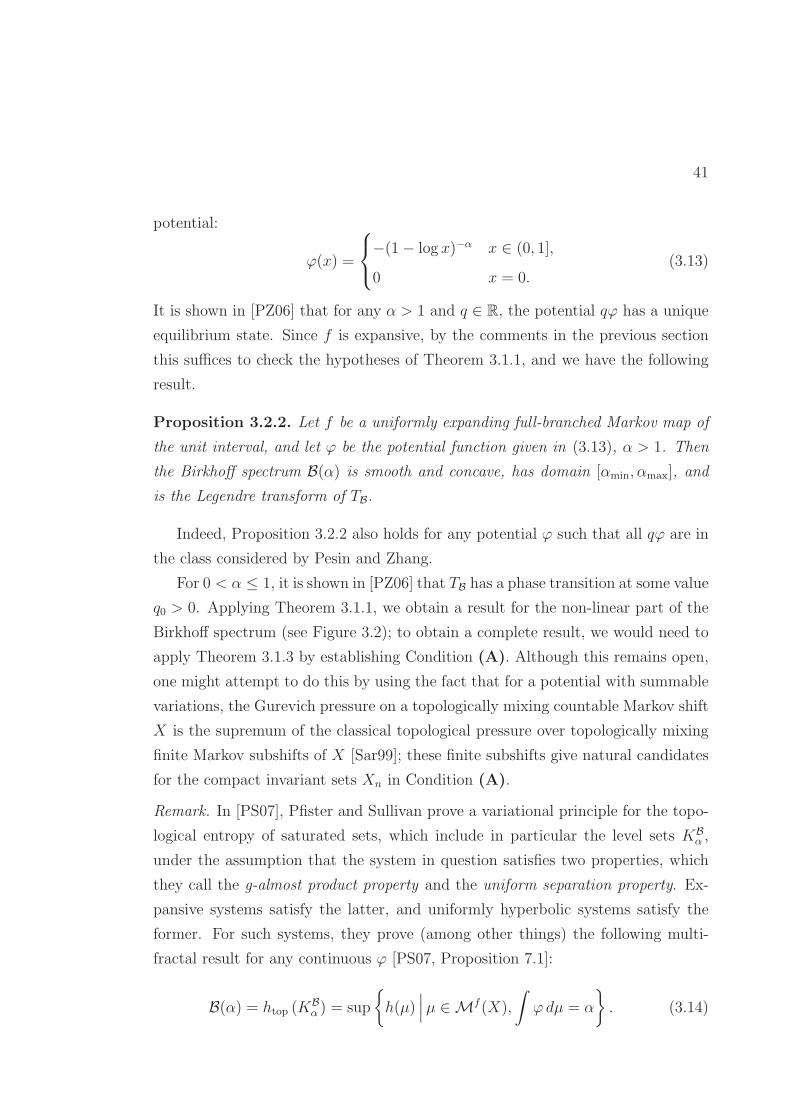
41
potential:
ϕ(x) =
−(1 − log x)−α x ∈ (0, 1],
0 x = 0.(3.13)
It is shown in [PZ06] that for any α > 1 and q ∈ R, the potential qϕ has a unique
equilibrium state. Since f is expansive, by the comments in the previous section
this suffices to check the hypotheses of Theorem 3.1.1, and we have the following
result.
Proposition 3.2.2. Let f be a uniformly expanding full-branched Markov map of
the unit interval, and let ϕ be the potential function given in (3.13), α > 1. Then
the Birkhoff spectrum B(α) is smooth and concave, has domain [αmin, αmax], and
is the Legendre transform of TB.
Indeed, Proposition 3.2.2 also holds for any potential ϕ such that all qϕ are in
the class considered by Pesin and Zhang.
For 0 < α ≤ 1, it is shown in [PZ06] that TB has a phase transition at some value
q0 > 0. Applying Theorem 3.1.1, we obtain a result for the non-linear part of the
Birkhoff spectrum (see Figure 3.2); to obtain a complete result, we would need to
apply Theorem 3.1.3 by establishing Condition (A). Although this remains open,
one might attempt to do this by using the fact that for a potential with summable
variations, the Gurevich pressure on a topologically mixing countable Markov shift
X is the supremum of the classical topological pressure over topologically mixing
finite Markov subshifts of X [Sar99]; these finite subshifts give natural candidates
for the compact invariant sets Xn in Condition (A).
Remark. In [PS07], Pfister and Sullivan prove a variational principle for the topo-
logical entropy of saturated sets, which include in particular the level sets KBα ,
under the assumption that the system in question satisfies two properties, which
they call the g-almost product property and the uniform separation property. Ex-
pansive systems satisfy the latter, and uniformly hyperbolic systems satisfy the
former. For such systems, they prove (among other things) the following multi-
fractal result for any continuous ϕ [PS07, Proposition 7.1]:
B(α) = htop (KBα ) = sup
{
h(µ)∣
∣
∣µ ∈ Mf (X),
∫
ϕdµ = α
}
. (3.14)

42
Given (3.14), it is not difficult to show that (3.6) holds, which establishes the
multifractal formalism for systems with the g-almost product property and uniform
separation, provided the potential is continuous. In particular, this includes the
example given above, as well as some (but by no means all) of the examples
mentioned below.
3.2.4 Non-uniform hyperbolicity
3.2.4.1 Parabolic maps
An important class of non-uniformly expanding maps is the Manneville–Pomeau
maps; these are non-uniformly expanding interval maps with an indifferent fixed
point. The primary potential of interest in this case is the geometric potential
log |f ′|, which corresponds to studying a non-Holder potential on a uniformly ex-
panding interval map via an appropriate change of coordinates; thus this is closely
related to the previous example.
The thermodynamic properties and Lyapunov spectra of these maps were stud-
ied in [PW99, Nak00, GR09]; once again, Theorem 3.1.1 provides a direct proof of
the multifractal results using the thermodynamic results, although as above, one
would need to establish Condition (A) to deal with the linear parts of the spectrum
using Theorem 3.1.3. We also remark that a significant achievement of [GR09] is
to deal with the endpoints of the spectrum (λ = 0 and λ = ∞), which cannot be
dealt with using the present results.
Moving to two (real) dimensions, let f : C → C be a parabolic rational map of
the Riemann sphere; that is, a rational map such that the Julia set J(f) contains
at least one indifferent fixed point (that is, a fixed point z0 for which |f ′(z0)| = 1),
but does not contain any critical points. Following Makarov and Smirnov [MS00],
we say that f is exceptional if there is a finite, non-empty set Σ ⊂ C such that
f−1(Σ) \ Crit f = Σ, where Crit f is the set of critical points of f .
Let ϕ(z) = log |f ′(z)| be the geometric potential. By combining the results
in [MS00] with [Hu08, Corollary D.1 and Theorem G], we see that if f is non-
exceptional, then the graph of the function TB is as shown in Figure 3.2. In
particular, TB is analytic and strictly convex on (q0,∞), where q0 = − dimH J(f),

43
and so writing
α1 = D+TB(q0), α2 = limq→∞
T ′B(q),
it follows from Theorem 3.1.1 that B(α) = TL1B on (α1, α2). Since we are dealing
with the geometric potential, this is also the entropy spectrum for Lyapunov ex-
ponents, and we may apply (1.8) to obtain the dimension spectrum for Lyapunov
exponents, LD(α) = 1αTL1B (α).
This result is obtained by other methods in [GPR09], where it is also shown
that the spectra are linear on [0, α1] (the dotted line in Figure 3.2). As before,
giving an alternate proof of this using Theorem 3.1.3 would require establishing
Condition (A).
Once again, Pfister and Sullivan’s results establish the multifractal formalism
for the Birkhoff spectrum here, but not for the dimension spectrum for Lyapunov
exponents, as they only consider topological entropy.
3.2.4.2 Maps with contracting regions
The existence and uniqueness of equilibrium states for a broad class of non-
uniformly expanding maps in a higher dimensional setting was studied by Oliveira
and Viana [OV08] and by Varandas and Viana [VV08]. To the best of the author’s
knowledge, the multifractal properties of these systems have not been studied at
all, and so they provide an ideal application of Theorem 3.1.1. It does not appear
to be known whether or not these systems, which may have contracting regions,
satisfy specification or any other property that would imply Pfister and Sullivan’s
g-almost product property, and so the results of [PS07] cannot be applied.
We describe the systems studied in [VV08] and use the results of that paper to
apply Theorem 3.1.1. Let M be a compact manifold of dimension m with distance
function d (more generally, Varandas and Viana consider metric spaces in which the
Besicovitch covering lemma holds). Let f : M → M be a local homeomorphism,
and let L(x) be a bounded function such that for every x ∈ M there exists a
neighbourhood Ux ∋ x such that fx = f |Ux: Ux → f(Ux) is invertible, with
d(f(y), f(z)) ≥1
L(x)d(y, z)

44
for all y, z ∈ Ux. Thus if L(x) < 1, then f is expanding at x, while if L(x) ≥ 1,
then L controls how much contraction can happen near x.
Assuming that every point has finitely many preimages, we write degx(f) =
#f−1(x). Assume also that level sets for the degree are closed and that M is
connected; then is it shown in [VV08] that up to considering some iterate fN of
f , we can assume that degx(f) ≥ ehtop (f) for all x.
The final conditions on the map f are as follows: there exist constants σ > 1
and L > 0 and an open region A ⊂M such that
(H1) L(x) ≤ L for every x ∈ A and L(x) ≤ σ−1 for all x ∈ M \ A, and L is close
to 1 (see [VV08] for precise conditions).
(H2) There exists k0 ≥ 1 and a covering P = {P1, . . . , Pk0} of M by domains of
injectivity for f such that A can be covered by r < ehtop (f) elements of P .
That is, f is uniformly expanding outside of A, and does not display too much
contraction inside A; furthermore, since there are at least ehtop (f) preimages of any
given point x, and only r of these can lie in covering of A by elements of P , every
point has at least one preimage in the expanding region.
The requirement on the potential ϕ is that
(P) ϕ : M → R is Holder continuous and supϕ− inf ϕ < htop (f) − log r.
It is proved in [VV08] that for any map f and potential ϕ satisfying these condi-
tions, there exists a unique equilibrium state for ϕ. In particular, if (P) holds for
ϕ, then there exists q0 > 1 such that (P) holds for qϕ as well, for all q ∈ (−q0, q0).
Thus Theorem 3.1.1 applies, and we have the following result on the Birkhoff
spectrum.
Proposition 3.2.3. Given a map f : M → M satisfying (H1) and (H2) and a
Holder continuous potential ϕ : M → R satisfying (P), there exists q0 > 1 such
that TB is C1 on the interval (−q0, q0), and writing
α1 = limq→−q+
0
T ′B(q), α2 = lim
q→q−0
T ′B(q),
we have B(α) = TL1B (α) = infq∈R(TB(q) − qα) for every α ∈ [α1, α2].

45
See [VV08] for examples of specific systems to which their conditions, and hence
Proposition 3.2.3, apply.
3.2.4.3 Maps with critical points
Ever since the family of logistic maps was introduced, unimodal and multimodal
maps have received a great deal of attention. Existence and uniqueness of equilib-
rium states for a certain class of bounded potentials were established in [BT08].
In particular, let H denote the collection of topologically mixing C∞ interval maps
f : [0, 1] → [0, 1] with hyperbolically repelling periodic points and non-flat critical
points; given f ∈ H, let ϕ : [0, 1] → R be a Holder continuous potential such that
supϕ− inf ϕ < htop (f). (3.15)
It is shown in [BT08] that there exists a unique equilibrium state for ϕ, and so the
analogue of Proposition 3.2.3 holds here.
In fact, it was shown by Blokh that any continuous topologically mixing interval
map has the specification property (see, for example, [Buz97]), which implies the g-
almost product property, and so Pfister and Sullivan’s result applies here, showing
that the multifractal formalism holds for any continuous potential ϕ on the entire
spectrum. However, their result does not apply to unbounded potentials such as
the geometric potential ϕ(x) = − log |f ′(x)|.
The potentials qϕ, where ϕ is the geometric potential, were studied in [PS08,
BT09, IT09b]. In the last of these papers, Iommi and Todd showed that for a
related class of maps f , the potential qϕ has a unique equilibrium state for all
q ∈ (−∞, 0]. (In fact, they obtain results for q > 0 as well, but we do not yet have
the tools to use these here.) Thus we may apply Theorem 3.1.5 and show that if
α0 = limq→0− T′B(q) and αmin = limq→−∞ T ′
B(q), then for all q ≤ 0, we have
TB(q) = supα∈R
(B(α) + qα),
and for all α ∈ [αmin, α0], we have
B(α) = infq∈R
(TB(q) − qα).

46
In particular, B(α) is strictly concave and C1 on [αmin, α0], and furthermore, KBα =
∅ for α < αmin.
3.3 Preparatory results
3.3.1 Convergence results
Proposition 3.3.1. Let X be a compact metric space, f : X → X be continuous,
and ϕ ∈ Af . Let µ ∈ Mf (X) be an invariant measure, and consider a sequence
of (not necessarily f -invariant) measures {µn} ⊂ M(X) such that µn → µ in the
weak* topology. Then
limn→∞
∫
ϕdµn =
∫
ϕdµ. (3.16)
Proof. If ϕ is continuous, then this is immediate. If ϕ ∈ Af is discontinuous, then
let M ∈ R be such that |ϕ(x)| ≤ M for all x ∈ X, and fix ε > 0. Condition (B)
in the definition of Af tells us that µ(C(ϕ)) = 0, and thus there exists an open
neighbourhood B ⊃ C(ϕ) such that µ(B) < ε. Since B is closed, we have
µ(B) ≥ limn→∞
µn(B),
and so there exists N such that µn(B) ≤ µn(B) < 2ε for all n ≥ N . Now we have
∣
∣
∣
∣
∫
X
ϕdµ−
∫
X
ϕdµn
∣
∣
∣
∣
≤
∣
∣
∣
∣
∫
X\B
ϕdµ−
∫
X\B
ϕdµn
∣
∣
∣
∣
+
∣
∣
∣
∣
∫
B
ϕdµ−
∫
B
ϕdµn
∣
∣
∣
∣
.
Since ϕ is continuous on the compact set X \ B, the first difference goes to 0 as
n → ∞. Furthermore, by the above estimates, the second difference is less than
3Mε. Since ε > 0 was arbitrary, this completes the proof of (3.16).
Observe that if X is a compact metric space and ψ : X → R ∪ {−∞} is con-
tinuous, then it must be bounded above (since it never takes the value +∞). We
use this fact in the next proposition.
Proposition 3.3.2. Let X be a compact metric space and ψ : X → R ∪ {−∞}
be continuous (and hence bounded above). Consider a sequence of measures {µn}

47
converging to µ in the weak* topology, and suppose that∫
ψ dµ > −∞. Then
∫
ψ dµ ≥ limn→∞
∫
ψ dµn. (3.17)
Proof. Given M < 0, define a continuous function ψM : X → R by
ψM(x) = max(ψ(x),M).
Because ψ is integrable with respect to µ, we have for every ε > 0 some M < 0
such that∫
(ψM − ψ) dµ < ε,
from which we deduce that
∫
ψ dµ ≥
∫
ψM dµ− ε = limn→∞
∫
ψM dµn − ε ≥ limn→∞
∫
ψ dµn − ε.
Because ε > 0 was arbitrary, this establishes (3.17).
Observe that there are no dynamics in Proposition 3.3.2, so there is no require-
ment that any of the measures µn or µ be invariant.
3.3.2 Measures associated with approximate level sets
Recall that the level sets KBα are defined by
KBα (ϕ) =
{
x ∈ X∣
∣
∣lim
n→∞
1
nSnϕ(x) = α
}
,
where we write KBα (ϕ) to emphasise the role of the function ϕ. This may be
rewritten as
KBα (ϕ) =
{
x ∈ X∣
∣
∣∀ε > 0∃N such that
∣
∣
∣
∣
1
nSnϕ(x) − α
∣
∣
∣
∣
< ε for all n ≥ N
}
=⋂
ε>0
⋃
N∈N
⋂
n≥N
{
x ∈ X∣
∣
∣
∣
∣
∣
∣
1
nSnϕ(x) − α
∣
∣
∣
∣
< ε
}
.

48
In the proofs of our main results, we will need to consider the following “approxi-
mate level sets”:
F ε,Nα (ϕ) =
⋂
n≥N
{
x ∈ X∣
∣
∣
∣
∣
∣
∣
1
nSnϕ(x) − α
∣
∣
∣
∣
< ε
}
F εα(ϕ) =
⋃
N∈N
F ε,Nα (ϕ).
(3.18)
For these we have
KBα (ϕ) =
⋂
ε>0
F εα(ϕ),
In particular, the following relations will be quite useful:
htop (KBα (ϕ)) ≤ htop (F ε
α(ϕ)) = supN
(
htop Fε,Nα (ϕ)
)
,
dimH(KBα (ϕ)) ≤ dimH(F ε
α(ϕ)) = supN
(
dimH Fε,Nα (ϕ)
)
.
Observe that for a continuous function ϕ, the sets F ε,Nα (ϕ) are obtained via a
sort of Cantor construction, being a countable intersection of sets {x ∈ X |
|(1/n)Snϕ(x) − α| < ε}. When Z is obtained via such a construction, it is rea-
sonable to approximate htop Z with ChtopZ, which gives us an upper bound. A
similar upper bound applies when we study the topological pressure.
The utility of the capacity quantities (entropy and pressure) for our purposes
is in the following lemma, which shows that when we deal with sets like F ε,Nα on
which the Birkhoff averages converge uniformly to a given range of values, then
we can build measures with large free energy and with the expected integrals.
Lemma 3.3.3. Let X be a compact metric space, f : X → X be continuous, and
ψ, ζ ∈ Af . Fix Z ⊂ X and let β1, β2 ∈ R be given by
β1 = limn→∞
infx∈Z
1
nSnψ(x), β2 = lim
n→∞supx∈Z
1
nSnψ(x).

49
Then for every γ > 0 there exists µ ∈ Mf (X) satisfying the following:
∫
ψ dµ ∈ [β1, β2], (3.19)
h(µ) +
∫
ζ dµ ≥ CPZ(ζ) − γ. (3.20)
Proof. The construction of µ satisfying (3.20) is given in part 2 of the proof
of [Wal75, Theorem 9.10], which is due to Misiurewicz, and goes as follows. Choose
δ > 0 such that
limn→∞
1
n
∑
x∈En
eSnζ(x) > CPZ(ζ) − γ,
where En is a maximal (n, δ)-separated set, and define an atomic measure σn on
En by
σn =
∑
y∈EneSnζ(y)δy
∑
z∈EneSnζ(z)
. (3.21)
Define µn by
µn =1
n
n−1∑
i=0
σn ◦ f−i, (3.22)
and let µ be any weak* limit of the sequence µn—then µ is invariant, and the
estimate (3.19) follows from Proposition 3.3.1 upon observing that for every ε > 0,
there exists N ∈ N such that∫
ψ dµn ∈ [β1 − ε, β2 + ε] for all n ≥ N . The
estimate (3.20) is shown in the proof in [Wal75]; although the proof there assumes
that ζ is continuous, this is only used to guarantee the convergence∫
ζ dµnj→
∫
ζ dµ, which in our case is given by Proposition 3.3.1.
The full strength of Lemma 3.3.3 is only needed in the proof of Theorem 5.2.2
(for the dimension spectrum). For the proof of Theorem 3.1.1 (for the Birkhoff
spectrum), we only need the case ζ = 0. In particular, in order to prove Theo-
rems 3.1.4 and 3.1.5, we only need the following two versions of Lemma 3.3.3.
Lemma 3.3.4. Let X be a compact metric space, f : X → X be continuous, and
ϕ : X → R be Borel measurable and bounded above and below. Suppose Z ⊂ X is
such that Chtop(Z) > Chtop(C(ϕ)). Fix Z ⊂ X and let β1, β2 ∈ [−∞,∞] be given
by
β1 = limn→∞
infx∈Z
1
nSnϕ(x), β2 = lim
n→∞supx∈Z
1
nSnϕ(x).

50
Then for every γ > 0 there exists µ ∈ Mf (X) satisfying the following:
∫
ϕdµ ∈ (β1 − γ, β2 + γ), (3.23)
h(µ) ≥ Chtop(Z) − γ. (3.24)
Proof. For n ∈ N and δ > 0, let P δn be the maximal cardinality of an (n, δ)-
separated subset of Z, and recall that
Chtop(Z) = limδ→0
limn→∞
1
nlogP δ
n .
In particular, decreasing γ if necessary, we may choose δ > 0 such that
Chtop(C(ϕ), δ) < Chtop(Z) − γ < limn→∞
1
nlogP δ
n . (3.25)
Writing h0 = limn→∞1n
logP δn , we choose η > 0 such that h0 − η > Chtop(C(ϕ), δ).
Thus there exists C > 0 such that for every m ∈ N there exists a set Fm ⊂ C(ϕ)
such that
#Fm ≤ Cem(h0−η) (3.26)
and Um =⋃
x∈FmB(x,m, δ) ⊃ C(ϕ). Observe that Um is open because f is con-
tinuous.
Given n ∈ N, let En be an (n, δ)-separated subset of Z with maximum cardi-
nality #En = P δn . Following the previous proof, consider the measures σn given
by (3.21) with ζ = 0:
σn =
∑
x∈Enδx
#En
. (3.27)
Now we vary the construction slightly; given 0 ≤ m < n, we go n −m steps (not
n) along each orbit:
µmn =
1
n−m
n−m−1∑
k=0
σn ◦ f−k. (3.28)
That is, µmn is a convex combination of δ-measures evenly distributed across the
first n−m points in each orbit that begins in En.

51
For every 0 ≤ k < n−m− 1, consider the set
Bmn (k) = {x ∈ En | fk ∈ Um} =
⋃
z∈Fm
f−k(B(z,m, δ)) ∩ En.
Observe that for every z ∈ Fm and every pair x 6= y ∈ f−k(B(z,m, δ))∩En, we have
d(f i(x), f i(y)) < δ for all n−m ≤ i < n, and since En is (n, δ)-separated, it follows
that d(f i(x), f i(y)) ≥ δ for some 0 ≤ i < n−m. In particular, f−k(B(z,m, δ)) ∩
En ⊂ Z is (n−m, δ)-separated, and hence has cardinality at most P δn−m. It follows
that
#Bmn (k) ≤ Cem(h0−η)P δ
n−m,
where C is as in (3.26), and hence
σn(f−k(Um)) =#Bm
n (k)
#En
≤ Ce−ηm+mh0P δ
n−m
P δn
.
This holds for all 0 ≤ k < n−m, and hence
µmn (Um) ≤ Ce−ηm e
mh0P δn−m
P δn
. (3.29)
Thus in order to bound µmn (Um), we need some control of the ratio P δ
n−m/Pδn .
Observe that if P δn is actually equal to enh0 for all n, then (3.29) immediately yields
the bound µmn (Um) ≤ Ce−ηm. However, P δ
n may not grow as uniformly as we would
like, so we must be more careful.
Given m ∈ N, consider the quantity
L(m) = limn→∞
(log(P δn) − log(P δ
n−m) −mh0).
Suppose L(m) < 0 for some m. Then there exists ε > 0 and N ∈ N such that for
all n ≥ N , we have
log(P δn) − log(P δ
n−m) −mh0 < −ε.
In particular, this gives the following for every k ∈ N:
log(P δN+km) < log(P δ
N) + kmh0 − kε.

52
Dividing by km and taking the limit as k → ∞, we get
h0 = limn→∞
1
nlog(P δ
n) ≤ limk→∞
1
N + km(P δ
N+km) < h0 −ε
m,
a contradiction. This proves that L(m) ≥ 0 for all m, from which we deduce that
for every m ∈ N, there exists a sequence nj = nj(m) → ∞ such that
limj→∞
(log(P δnj
) − log(P δnj−m) −mh0) ≥ 0,
or equivalently,
limj→∞
P δnj
emh0P δnj−m
≥ 1. (3.30)
In combination with (3.29), this will soon give us the bound we need.
As in the proof of Lemma 3.3.3, let µm be a weak* limit point of the sequence µmnj
(by passing to a subsequence if necessary, we assume that µmnj
→ µm). Invariance
of µm and the entropy estimate (3.24) hold just as before, so it only remains to
show (3.23).
Let M = supx∈X |ϕ(x)|, and choose m large enough so that Ce−ηm < γ/2M .
Carry out the above construction for this value of m, and observe that because Um
is open, we have
µm(Um) ≤ limnj→∞
µmnj
(Um) ≤ Ce−ηm <γ
2M, (3.31)
where the middle inequality follows from (3.29) and (3.30). Consequently,
∣
∣
∣
∣
∫
X
ϕdµm −
∫
X
ϕdµmnj
∣
∣
∣
∣
≤
∣
∣
∣
∣
∫
X\Um
ϕdµm −
∫
X\Um
ϕdµmnj
∣
∣
∣
∣
+
∣
∣
∣
∣
∫
Um
ϕdµm −
∫
Um
ϕdµmnj
∣
∣
∣
∣
. (3.32)
Since ϕ is continuous on the compact set X \ Um, the first difference goes to 0
as j → ∞, and by (3.31), the second term is less than γ; this proves (3.23) for
µm.
Lemma 3.3.5. Let X be a compact metric space, let f : X → X be continuous,

53
and let ψ : X → R∪ {−∞} be continuous (and hence bounded above). Fix Z ⊂ X
and let β ∈ R be given by
β = limn→∞
infx∈Z
1
nSnψ(x).
Then for every γ > 0 there exists µ ∈ Mf (X) satisfying the following:
∫
ψ dµ ≥ β, (3.33)
h(µ) ≥ Chtop(Z) − γ. (3.34)
Proof. The proof is exactly as in Lemma 3.3.3 with the choice ζ = 0, η = ψ, with
Proposition 3.3.2 taking the place of Proposition 3.3.1.
3.4 Proof of Theorem 3.1.1
The proof of Theorem 3.1.1 proceeds in three parts, corresponding to the three
parts of the theorem. In the first part, we show that TB is the Legendre transform of
B, thus establishing (3.3). From this, it immediately follows by standard properties
of the Legendre transform that TL1B is the concave hull of B; that is, it is the smallest
concave function greater than or equal to B at all α.
Part II of the theorem is an easy consequence of the following proposition.
Proposition 3.4.1. Suppose that KBα is non-empty; that is, there exists x ∈ X
such that ϕ+(x) = limn→∞1nSnϕ(x) = α. Then P ∗(qϕ) ≥ αq for all q ∈ R.
Once Part I is established, Part III of the theorem is proved via the following
series of intermediate results.
Proposition 3.4.2. Let ϕ be Borel measurable and suppose that νq is an ergodic
equilibrium state for qϕ. Let α =∫
ϕdνq. Then
B(α) ≥ TL1B (α). (3.35)
Note the requirement in Proposition 3.4.2 that the equilibrium state νq be
ergodic. It will often be the case that general arguments will give the existence

54
of non-ergodic equilibrium states with α(νq) = α, but this is not sufficient for our
purposes.
The following important result is well-known.
Proposition 3.4.3 (Ruelle’s formula for the derivative of pressure). Let ψ and φ
be Borel measurable functions. If the function
q 7→ P ∗(ψ + qφ)
is differentiable at q, and if in addition νq is an equilibrium state for ψ + qφ, then
d
dqP ∗(ψ + qφ) =
∫
X
φ dνq. (3.36)
Corollary 3.4.4. Suppose TB is continuously differentiable on (q1, q2) and qϕ has
an equilibrium state νq for each q ∈ (q1, q2). Let α1 = D+TB(q1) and α2 =
D−TB(q2); then for every α ∈ (α1, α2) there exists q ∈ R such that qϕ has an
ergodic equilibrium state νq with α =∫
ϕdνq.
Once these results are established, (3.6) is a direct consequence of Proposi-
tion 3.4.2 and Corollary 3.4.4. It then follows from basic properties of the Legen-
dre transform that B = TL1B has the same regularity as TB (except for values of α
corresponding to intervals on which TB is affine).
Proof of part I. We prove (3.3) by establishing the following two inequalities:
TB ≤ BL2 , (3.37)
TB ≥ BL2 . (3.38)
First we prove (3.37). Recall that
TB(q) = P ∗(qϕ) = supν∈Mf
E(X)
{
h(ν) + q
∫
X
ϕdν
}
.
By Birkhoff’s ergodic theorem, every ergodic measure ν has ν(KBα ) = 1 for some
α, and so for ν-almost every x ∈ KBα (in particular, for some x ∈ KB
α ), we have

55
∫
Xϕdν = ϕ+(x) = α. It follows that
TB(q) = supα∈R
(
supν∈Mf
E(KB
α )
{
h(ν) + q
∫
X
ϕdν
}
)
≤ supα∈R
(
htop (KBα ) + qα
)
= BL2(q),
where the inequality h(ν) ≤ htop (KBα ) follows from Theorem A2.1 in [Pes98].
Now we prove the reverse inequality (3.38), by showing that TB(q) = P ∗(qϕ) ≥
B(α) + qα for all q, α ∈ R. To this end, we fix ε > 0 and consider the sets F εα, F ε,N
α
defined in (3.18).
Applying Lemma 3.3.3 with ζ = 0, ψ = ϕ, Z = F ε,Nα , and some γ > 0, we
obtain a measure µ ∈ Mf (X) with h(µ) ≥ Chtop(F ε,Nα ) − γ and
∫
ϕdµ ≥ α − ε.
It follows that
P ∗(qϕ) ≥ h(µ) + q
∫
ϕdµ ≥ Chtop(F ε,Nα ) − γ + qα− qε,
and since Lemma 3.3.3 can be applied with arbitrarily small γ, we get
P ∗(qϕ) ≥ htop (F ε,Nα ) + qα− qε.
Taking the supremum over all N yields
P ∗(qϕ) ≥ htop (F εα) + qα− qε ≥ htop (KB
α ) + qα− qε,
and since ε > 0 was arbitrary, this implies
P ∗(qϕ) ≥ htop (KBα ) + qα.
This holds for all q, α ∈ R, which establishes (3.38).
We now proceed to the proof of Part II.
Proof of Proposition 3.4.1. Suppose α ∈ R is such that there exists x ∈ KBα . Con-

56
sider the empirical measures
µn,x =n−1∑
i=0
δf i(x).
Choose any subsequence nk such that µnk,x converges in the weak* topology to some
µ ∈ Mf (X). Then by Proposition 3.3.1, we have∫
ϕdµ = α, and in particular,
P ∗(qϕ) ≥ h(µ) +
∫
qϕ dµ ≥ q
∫
ϕdµ ≥ qα
for every q ∈ R.
Finally, we prove the string of propositions which implies Part III.
Proof of Proposition 3.4.2. Observe that since νq is ergodic, we have νq(KBα ) = 1,
and hence h(νq) ≤ htop (KBα ). Thus
TL1B (α) = inf
q′∈R
(TB(q′) − q′α′)
≤ TB(q) − qα′ = P ∗(qϕ) − qα
= h(νq) +
∫
X
qϕ dνq − qα
≤ htop (KBα ) = B(α).
Proof of Proposition 3.4.3. Write g(q′) = P ∗(ψ + q′φ). Then for all q′ ∈ R, we
have
g(q′) = P ∗(ψ + q′φ)
= supν
{
h(ν) +
∫
X
ψ dν +
∫
X
q′φ dν
}
≥ h(νq) +
∫
X
ψ dνq + q′∫
X
φ dνq
= P ∗(ψ + qφ) + (q′ − q)
∫
X
φ dνq,
= g(q) + (q′ − q)
∫
X
φ dνq,

57
whence
g(q′) − g(q) ≥ (q′ − q)
∫
X
φ dνq.
In particular, for q′ > q, we get
g(q′) − g(q)
q′ − q≥
∫
X
φ dνq,
and hence g′(q) ≥∫
Xφ dνq (recall that differentiability of g was one of the hy-
potheses of the theorem), while for q′ < q,
g(q′) − g(q)
q′ − q≤
∫
X
φ dνq,
and hence g′(q) ≤∫
Xφ dνq, which establishes equality.
Proof of Corollary 3.4.4. Since T ′B is continuous, the Intermediate Value Theorem
implies that for every such α there exists q such that T ′B(q) = α. Thus applying
Proposition 3.4.3 with ψ = 0 and φ = ϕ, we see that any equilibrium state ν for
qϕ has ν(qϕ) = α. Choose some such ν; if ν is not ergodic, then any element in
its ergodic decomposition is also an equilibrium state, and we are done.
3.5 Proof of Theorems 3.1.3, 3.1.4, and 3.1.5
Given the proof of Theorem 3.1.1 in the previous section, the proofs of Theo-
rems 3.1.3, 3.1.4, and 3.1.5 are relatively straightforward.
Proof of Theorem 3.1.3. Recall that the first two parts of Theorem 3.1.1 hold with-
out any assumptions on f , and thus we already have TB = BL2 . It remains only to
show that B(α) ≥ TL1B (α) for every α ∈ [αmin, αmax], given Condition (A).
Given such an α, if there exists q ∈ R such that T ′B(q) = α, then the proof of
Theorem 3.1.1 shows that B(α) = TL1B (α). Thus we suppose that no such q exists;
in this case, let q0 = Q(α) be the (unique) value of q such that
TB(q) ≥ TB(q0) + (q − q0)α
for all q ∈ R. (Equivalently, we have q0 = −(TL1B )′(α).)

58
Applying Theorem 3.1.1 to the subsystem Xn, we see that
htop (KBα ∩Xn) = inf
q∈R
(P ∗Xn
(qϕ) − qα);
since q 7→ P ∗Xn
(qϕ) is assumed to be differentiable on R, for every α ∈ [αmin, αmax]
there exists qn ∈ R such that An(qn) = ddqP ∗
Xn(qϕ)|q=qn
= α. Let µn be an ergodic
equilibrium state for qnϕ on Xn; then∫
ϕdµn = α by Proposition 3.4.3, and so
µn(KBα ) = 1. Thus we have
htopKBα ≥ h(µn) = P ∗
Xn(qnϕ) − qnα. (3.39)
It follows from convexity of the pressure function that qn → q0 as n goes to ∞,
and by continuity of the pressure function and Condition (A), this implies that
limn→∞
P ∗Xn
(qnϕ) = P ∗(q0ϕ),
which together with (3.39) shows that B(α) ≥ TB(q0) − q0α ≥ TL1B (α).
Proof of Theorem 3.1.4. The proof of Theorem 3.1.4 mirrors the proof of Theo-
rem 3.1.1; the primary difference is that Lemma 3.3.4 replaces Lemma 3.3.3 in the
proof of Part I, where we show (3.9).
The proof of Proposition 3.4.1 does not go through in this setting, and so Part
II is weakened from the corresponding statement in Theorem 3.1.1.
The series of propositions in Part III goes through unchanged, as Proposi-
tion 3.4.2, Proposition 3.4.3, and Corollary 3.4.4 all hold without regard to conti-
nuity of the potential ϕ.
Observe that (3.37) holds here as well without modification, since its proof does
not require any hypotheses on ϕ. Thus to prove (3.9), it suffices to establish the
following inequality for every q ∈ IQ(h0):
TB(q) ≥ supα∈IA(h0)
(B(α) + qα). (3.40)
That is, we show that TB(q) = P ∗(qϕ) ≥ B(α) + qα for all q ∈ IQ(h0) and
α ∈ IA(h0). Observe that if B(α) ≤ h0, then since α ∈ IA(h0) we have TL1B (α) =

59
infq∈R(TB(q) − qα) > h0 ≥ B(α), and so in particular TB(q) ≥ B(α) + qα for
q ∈ IQ(h0). Thus it remains only to consider the case B(α) > h0.
As in the proof of (3.38) in Theorem 3.1.1, we fix ε > 0 and consider the sets F εα,
F ε,Nα defined in (3.18). Because h0 < B(α) = htopK
Bα ≤ htop F
εα = supN htop F
ε,Nα ,
we can find N ∈ N such that htop Fε,Nα > h0, and then apply Lemma 3.3.4 with ψ =
ϕ, Z = F ε,Nα , and some γ > 0 to obtain a measure µ with h(µ) ≥ Chtop(F ε,N
α ) − γ
and∫
ϕdµ ≥ α− ε− γ. It follows that
P ∗(qϕ) ≥ h(µ) + q
∫
ϕdµ ≥ Chtop(F ε,Nα ) − γ + qα− q(ε+ γ),
and since Lemma 3.3.4 can be applied with arbitrarily small γ, we get
P ∗(qϕ) ≥ htop (F ε,Nα ) + qα− qε.
Taking the supremum over all such N yields
P ∗(qϕ) ≥ htop (F εα) + qα− qε ≥ htop (KB
α ) + qα− qε,
and since ε > 0 was arbitrary, this implies
P ∗(qϕ) ≥ htop (KBα ) + qα.
This holds for all q ∈ IQ(h0) and α ∈ IA(h0), which establishes (3.40).
For Part II of Theorem 3.1.4, we observe that if B(α) > h0, then we can apply
Lemma 3.3.4 exactly as above to obtain TB(q) ≥ B(α) + qα for all q ∈ R, and
hence TL1B (α) ≥ B(α) > h0 as well, so α ∈ IA(h0).
As remarked above, the propositions in Part III go through unchanged, and we
are done.
Proof of Theorem 3.1.5. The proof of Parts I of Theorem 3.1.5 is nearly identical
to the proof of Theorem 3.1.4, with Lemma 3.3.5 replacing Lemma 3.3.4 in the
proof of (3.3), and with (−∞, 0) and (−∞, α0] replacing IQ(h0) and IA(h0).
Part II of Theorem 3.1.5 follows from the observation that Proposition 3.4.1
does apply in this setting as follows: if KBα is non-empty for some α ∈ R, then
P ∗(qϕ) ≥ αq for all q ≤ 0. The proof only requires replacing Proposition 3.3.1

60
with Proposition 3.3.2.
Again, (3.37) holds here without modification. Furthermore, for any q ≤ 0 and
α ∈ R, we may fix ε > 0 and apply Lemma 3.3.5 with ψ = qϕ, Z = F ε,Nα , and
some γ > 0 to obtain a measure µ ∈ Mf (X) with h(µ) ≥ Chtop(F ε,Nα ) − γ and
∫
qϕ dµ ≥ qα− qε. It follows that
P ∗(qϕ) ≥ h(µ) +
∫
qϕ dµ ≥ Chtop(F ε,Nα ) − γ + qα− qε,
and just as in the proof of Theorem 3.1.1, we obtain
P ∗(qϕ) ≥ htop (KBα ) + qα.
This holds for all q ≤ 0 and α ∈ R, which establishes (3.38).
Part III is once again just as before.

Chapter 4Conformal maps and Bowen’s
equation
4.1 Pressure and dimension: known results
In order to establish multifractal results for spectra defined using Hausdorff dimen-
sion, we need to obtain a relationship between topological pressure and Hausdorff
dimension. The first such connection was given by Bowen [Bow79], who showed
that for certain compact sets (quasi-circles) J ⊂ C which arise as invariant sets of
fractional linear transformations f of the Riemann sphere, the Hausdorff dimension
t = dimH J is the unique root of the equation
PJ(−tϕ) = 0, (4.1)
where PJ is the topological pressure of the map f : J → J , and ϕ is the geometric
potential ϕ(z) = log |f ′(z)|. Later, Ruelle showed that Bowen’s equation (4.1) gives
the Hausdorff dimension of J whenever f is a C1+ε conformal map on a Riemannian
manifold and J is a repeller. More precisely, he proved the following [Rue82,
Proposition 4]:
Theorem 4.1.1. Let M be a Riemannian manifold and V ⊂ M be open, and
let f : V → M be C1+ε and conformal (that is, Df(x) is a scalar multiple of an
isometry for every x ∈ V ). Suppose J ⊂ V is a repeller—that is, it has the
following properties:

62
(1) J is compact.
(2) J is maximal: J = {x ∈ V | fn(x) ∈ V for all n > 0}.
(3) f is topologically mixing on J : For every open set U ⊂ V such that U ∩J 6= ∅,
there exists n such that fn(U) ⊃ J .
(4) f is uniformly expanding on J : There exist C > 0 and r > 1 such that
‖Dfnv‖ ≥ Crn‖v‖ for every tangent vector v ∈ TxM and every n ≥ 1.
Let ϕ(x) = log ‖Df(x)‖. Then Bowen’s equation (4.1) has a unique root, and this
root is equal to the Hausdorff dimension of J .
This result was eventually extended to the case where f is C1 by Gatzouras and
Peres [GP97]. One can also give a definition of conformal map in the case where X
is a metric space (not necessarily a manifold), and the analogue of Theorem 4.1.1
in this setting was proved by Rugh [Rug08].
In all of these settings, one of the essential tools is the availability of geometric
bounds that relate statically defined metric balls B(x, r) (used in the definition of
dimension) to dynamically defined Bowen balls B(x, n, δ) (used in the definition
of pressure). However, the above proofs differ in how these bounds are used. The
proofs given by Bowen, Ruelle, and Gatzouras and Peres all rely on the construction
of a measure of full dimension (in particular, a measure that is equivalent to
Hausdorff measure), which in turn relies on the aforementioned geometric bounds
(among other things). Rugh’s proof, on the other hand, does not use measures and
instead applies these bounds directly to the definitions of dimension and pressure.
These two methods of proof represent different approaches to the problem of
using Bowen’s equation to find the Hausdorff dimension of dynamically significant
sets. In this chapter, we will follow the second approach (Rugh’s) and avoid the
use of measures; this will allow us to establish the analogue of Theorem 4.1.1 for a
broad class of subsets of a repeller on which we may not have uniform expansion,
and which need not carry any invariant measures. First, however, we will mention
some of the other settings in which the approach using measures of full dimension
has been successful.
Working with maps in one real dimension, Urbanski [Urb96] proved that the
smallest root of (4.1) gives the Hausdorff dimension of a repeller J that is expand-

63
ing except on some set of indifferent fixed points, by finding a conformal measure
that is the measure of full dimension. Similar results for Julia sets of maps in
one complex dimension were proved in [DU91, Urb91]. In fact, Bowen’s equa-
tion is also known to give the Hausdorff dimension of the Julia set for a broad
class of rational maps (those satisfying the topological Collet-Eckmann condition)
whose Julia sets even contain critical points [PRLS03, PRLS04]. There are also
situations where conformal measures can be built when J is a non-compact set;
for instance, when J is the radial Julia set of a meromorphic function satisfying
certain conditions [UZ04, MU08, MU10].
Given a map f , all of the above results give the Hausdorff dimension of one very
particular dynamically significant set J via Bowen’s equation. It is natural to ask
if one can find the Hausdorff dimension of subsets Z ⊂ J via a similar approach.
For certain subsets, results in this direction are given by the multifractal anal-
ysis. In the uniformly expanding case, the multifractal results in [BPS97, PW97,
Wei99] all boil down to the following result. If J is a conformal repeller and
ϕ : J → R is any Holder continuous function, then for the one-parameter family of
sets Kα ⊂ J given by
Kα =
{
x ∈ J∣
∣
∣lim
n→∞
Snϕ(x)
Sn log ‖Df(x)‖= α
}
,
we may define a convex analytic function T : R → R implicitly by
PJ(qϕ− T (q) log ‖Df‖) = 0, (4.2)
and obtain dimH Kα as the Legendre transform of T :
dimH Kα = infq∈R
(T (q) − qα). (4.3)
In the case ϕ ≡ 0, α = 0, this reduces to Bowen’s equation; for other values of ϕ and
α, this may be seen as a sort of (indirect) generalisation of Theorem 4.1.1. Analo-
gous results for certain almost-expanding conformal maps with neutral fixed points
are at the heart of the multifractal analyses in [PW99, Nak00, GR09, GPR09,
MU10].
Once again, these results all rely on the construction of measures of full di-

64
mension on the sets Kα as Gibbs states νq for the family of potentials qϕ −
T (q) log ‖Df‖, and so they do not generalise to more arbitrary subsets Z ⊂ J
(which may not support any invariant measures). A more natural generalisation of
Theorem 4.1.1 would be to obtain dimH Z as the root of PZ(−t log ‖Df‖) = 0 using
Pesin and Pitskel’s notion of topological pressure on the set Z as a Caratheodory
dimension characteristic. Such a generalisation is the goal of this chapter; this
will allow us to prove the above multifractal results in a more general setting in
Chapter 5, where the measures νq are only required to be equilibrium states, and
not necessarily Gibbs.
Using the general theory of Caratheodory dimension characteristics introduced
in [Pes98], Barreira and Schmeling [BS00] introduced the notion of the u-dimension
dimu Z for positive functions u, showing that dimu Z is the unique number t such
that PZ(−tu) = 0. They also showed that for a subset Z of a conformal repeller
J , where we may take u = log ‖Df‖ > 0, we have dimu Z = dimH Z, and hence
upon replacing PJ with PZ , the Hausdorff dimension of any subset Z ⊂ J is given
by Bowen’s equation, whether or not Z is compact or invariant.
Thus it has already been shown that in the uniformly expanding case, Theo-
rem 4.1.1 holds not just for J itself, but for any subset Z ⊂ J . Furthermore, the
aforementioned works of Urbanski et al show that when we consider J itself, there
are many cases in which the requirement that f be uniformly expanding can be
replaced with rather weaker expansion properties. However, there do not appear
to be any results at present that combine these two directions, and give a Bowen’s
equation result for arbitrary sets Z under properties weaker than uniform expan-
sion (the closest results to this appear to be the multifractal results mentioned
above). We give such a result in this chapter, showing that the applicability of
Bowen’s equation to arbitrary Z extends beyond the uniformly expanding case.
Indeed, given a conformal map f without critical points or singularities, the
only requirement we place on the expansion properties of f is that every point x
of Z has positive lower Lyapunov exponent, and that there not be too much con-
traction along the orbit of x (see (4.5) below—this is automatically satisfied if the
Lyapunov exponent of x exists or if f is nowhere contracting). We do not require
any uniformity in these hypotheses; Z may contain points with arbitrarily small
or large Lyapunov exponents. Furthermore, these hypotheses are only required to

65
hold at points in Z, and not for other points in phase space.
This result has an immediate application to the multifractal formalism, as al-
ready mentioned in Section 3.2.2 and the sections following it (see also (1.8)): for
any conformal map without critical points or singularities (no expansion proper-
ties are required), it allows us to compute the dimension spectrum for Lyapunov
exponents directly from the entropy spectrum for Lyapunov exponents, which can
in turn be obtained from the pressure function, provided the latter has nice prop-
erties, as described in Chapter 3. Furthermore, we will use this result in Chapter 5
to compute the dimension spectrum for pointwise dimensions given certain ther-
modynamic information.
4.2 Definitions and statement of result
We consider a continuous map f acting on a compact metric space X.
Definition 4.2.1. We say that f : X → X is conformal with factor a(x) if for
every x ∈ X we have
a(x) = limy→x
d(f(x), f(y))
d(x, y), (4.4)
where a : X → [0,∞) is continuous. We denote the Birkhoff sums of log a by
λn(x) =1
nSn(log a)(x) =
1
n
n−1∑
k=0
log a(fk(x));
the lower and upper limits of this sequence are the lower Lyapunov exponent and
upper Lyapunov exponent, respectively:
λ(x) = limn→∞
λn(x), λ(x) = limn→∞
λn(x).
If the two agree (that is, if the limit exists), then their common value is the
Lyapunov exponent :
λ(x) = limn→∞
λn(x).
Because a is assumed to be continuous on a compact space X, it is bounded above
(and hence λ(x) is as well); we do not allow maps with singularities.

66
If a(x) = 0, then we say that x is a critical point for the map f . We will exclude
such points from the maps we consider.
Note that in the case where X is a smooth Riemannian manifold, the definition
of conformality may be restated as the requirement that Df(x) is a(x) times
some isometry, and the definition of Lyapunov exponent becomes the usual one
from smooth ergodic theory. In particular, if X is one-dimensional, then any
differentiable map is conformal.
We relate the Hausdorff dimension of Z to the topological pressure of log a on
Z, provided every point in Z has positive lower Lyapunov exponent and satisfies
the following tempered contraction condition:
infn∈N
0≤k≤n
{Sn−k log a(fk(x)) + nε} > −∞ for every ε > 0. (4.5)
Denote by B the set of all points in X which satisfy (4.5). The following three
criteria are useful for checking that x ∈ B.
1. Proposition 4.4.3 shows that if the Lyapunov exponent of x exists and is
positive—that is, if λ(x) = λ(x) > 0—then x satisfies (4.5).
2. If a(x) ≥ 1 for all x ∈ X, then (4.5) is automatically satisfied for all x ∈ X,
and so in this case B = X.
3. We say that x has bounded contraction if inf{Sn−k log a(fk(x)) | n ∈ N, 0 ≤
k ≤ n} > −∞. Any such point x satisfies (4.5).
Given E ⊂ R, we denote by A(E) the set of points along whose orbits all the
asymptotic exponential expansion rates of the map f lie in E:
A(E) = {x ∈ X | [λ(x), λ(x)] ⊂ E}.
In particular, A((0,∞)) is the set of all points for which λ(x) > 0. Our main
result deals with subsets Z ⊂ X that lie in both A((0,∞)) and B. (Observe that
by Proposition 4.4.3, A(α) = A({α}) ⊂ B for every α > 0.)
Theorem 4.2.1. Let X be a compact metric space and f : X → X be continuous
and conformal with factor a(x). Suppose that f has no critical points and no

67
singularities—that is, that 0 < a(x) <∞ for all x ∈ X. Consider Z ⊂ A((0,∞))∩
B. Then the Hausdorff dimension of Z is given by
dimH Z = t∗ = sup{t ≥ 0 | PZ(−t log a) > 0}
= inf{t ≥ 0 | PZ(−t log a) ≤ 0}.(4.6)
Furthermore, if Z ⊂ A((α,∞)) ∩ B for some α > 0 (that is, the lower Lyapunov
exponents of points in Z are uniformly positive), then t∗ is the unique root of
Bowen’s equation
PZ(−t log a) = 0. (4.7)
Finally, if Z ⊂ A(α) for some α > 0, then PZ(−t log a) = htop Z − tα, and hence
dimH Z =1
αhtop Z. (4.8)
Before proceeding to specific examples and to the proofs, we make a few remarks
on Theorem 4.2.1 in some standard settings.
1. For expanding conformal maps (a(x) > 1 for all x), we have B = X, and
Theorem 4.2.1 reduces to Barreira and Schmeling’s generalisation of Theo-
rem 4.1.1, although we work in the slightly more general setting where X
need not be a manifold.
2. For almost expanding conformal maps (maps which are expanding away from
a collection of indifferent periodic points), we have a(x) ≥ 1 for all x, and so
B = X; thus the theorem applies, showing that Bowen’s formula gives the
Hausdorff dimension of any set which does not contain any points with zero
lower Lyapunov exponent. This complements the results in [DU91, Urb91,
Urb96], which give the Hausdorff dimension of the entire Julia set for a
large family of almost expanding conformal maps, but have nothing to say
about arbitrary subsets of the Julia set. (Observe that because the Julia set
contains points with zero Lyapunov exponent, Theorem 4.2.1 does not give
the Hausdorff dimension of the entire Julia set.)
3. For maps with some contracting regions (a(x) < 1) but no critical points
(a(x) = 0), we cannot rule out the possibility that B 6= X. However, the

68
result still holds for Z ⊂ X as long as every point x ∈ Z satisfies (4.5) and has
positive lower Lyapunov exponent. In particular, if the Lyapunov exponent
is constant and positive on Z, then (4.8) relates the Hausdorff dimension of
Z to the topological entropy of Z; this proves the equality claimed earlier
in (1.8).
4.3 Applications
4.3.1 Lyapunov spectra
The dimension spectrum for Lyapunov exponents of a conformal repeller was stud-
ied by Weiss [Wei99], who proved that it is real analytic on an interval (α1, α2),
and may be obtained in terms of the Legendre transform of the pressure function.1
The proof in [Wei99] is roundabout, and analyses LD(α) in terms of the di-
mension spectrum for pointwise dimensions of a measure of maximal entropy, by
showing that for such a measure the level sets of the pointwise dimension coincide
with the level sets of the Lyapunov exponent (this may also be shown using the
fact that the local entropy of such a measure is constant everywhere and applying
Lemma 4.4.4 below), and then applying results from [PW97].
By using Theorems 3.1.1 and 4.2.1, we obtain a more direct proof of this re-
sult. When f is a C1+ε expanding conformal map on a repeller J , it is well-known
that the pressure function T : t 7→ PJ(−t log a) is real analytic and strictly convex
(provided log a is not cohomologous to a constant, or equivalently, that the mea-
sure of maximal dimension and the measure of maximal entropy do not coincide).
Then Theorem 3.1.1 applies to the entropy spectrum for Lyapunov exponents, and
Theorem 4.2.1 applies to the level sets KLα : together, they give a more direct proof
of the following well-known result.
Proposition 4.3.1. Let f : V → M be as in Theorem 4.1.1, and let J be a uni-
formly expanding repeller. Then the Lyapunov spectra of f are given in terms of
1Weiss also claims that the spectrum is concave, but Iommi and Kiwi have shown that thereare examples in which this is not the case [IK09].

69
the Legendre transform of the pressure function as follows:
LE(α) = inft∈R
(PJ(−t log a) − αt),
LD(α) =1
αinft∈R
(PJ(−t log a) − αt).(4.9)
In particular, if log a is not cohomologous to a constant, then the spectrum LE
is strictly concave, and both spectra are real analytic (this follows from analyticity
of the pressure function and standard properties of the Legendre transform).
For non-uniformly expanding conformal repellers, such as Manneville–Pomeau
maps and parabolic rational maps, this approach gives the partial results described
in Section 3.2.4.1. (To obtain the complete results given in [GPR09], we would
need to apply Theorem 3.1.3.)
4.3.2 Symbolic dynamics
We now describe a class of systems to which these results may be applied, for
which the phase space is not a manifold. Fix an integer k ≥ 2, and let X = Σ+k
be the full one-sided shift on k symbols. Given x, y ∈ X, let x ∧ y denote the
common prefix of x and y—that is, if n is the unique integer such that xi = yi for
all 1 ≤ i ≤ n, but xn+1 6= yn+1, then
x ∧ y = x1 . . . xn = y1 . . . yn.
Let ψ :⋃
n≥0{1, . . . , k}n → R+ be a function defined on the space of all finite words
on the alphabet {1, . . . , k}, and suppose that ψ is such that for every x ∈ X, the
sequence {ψ(x1 . . . xn)} is non-increasing and approaches 0 as n → ∞. Then
d(x, y) = ψ(x∧y) defines a metric on X = Σ+k ; to prove this, one needs only verify
the triangle inequality, or equivalently, show that
ψ(x ∧ z) ≤ ψ(x ∧ y) + ψ(y ∧ z)
for every x, y, z ∈ X. This follows from the observation that if n is the length of
the common prefix of x and z, then either xn+1 6= yn+1 or yn+1 6= zn+1: without

70
loss of generality, suppose the first holds, and then we have
ψ(x ∧ y) = ψ(x1 . . . xm) ≥ ψ(x1 . . . xn) = ψ(x ∧ z)
for some 0 ≤ m ≤ n. Thus d is a metric, and the requirement that ψ(x1 . . . xn) → 0
guarantees that d induces the product topology on X = {1, . . . , k}N.
In order for the shift σ to be conformal, we require the following limit to exist
for every x ∈ X:
a(x) = limn→∞
ψ(x2 . . . xn)
ψ(x1 . . . xn). (4.10)
Furthermore, we demand that a(x) depend continuously on x. If these conditions
are satisfied, then the shift σ is conformal with factor a(x) given by (4.10): indeed,
given any x, y ∈ X such that the length of the common prefix is n, we have
d(σ(x), σ(y))
d(x, y)=ψ(σ(x) ∧ σ(y))
ψ(x ∧ y)=ψ(x2 . . . xn)
ψ(x1 . . . xn),
and since y → x if and only if n→ ∞, this gives
limy→x
d(σ(x), σ(y))
d(x, y)= lim
n→∞
ψ(x2 . . . xn)
ψ(x1 . . . xn)= a(x).
Given the above conditions, we may apply Theorem 4.2.1 to subsets Z ⊂
X on which the lower Lyapunov exponents are positive and we have tempered
contraction. We now describe some simple candidates for the function ψ, for which
the results take on a straightforward form (and for which tempered contraction is
automatic).
Example 4.3.2. Fix θ > 1 and let ψ(x1 . . . xn) = θ−n, so that d(x, y) = θ−n, where
n + 1 is the first entry in which x and y differ. Then a(x) = θ for every x ∈ X,
and it follows from (4.8) that for every Z ⊂ X, we have
dimH Z =htop Z
log θ.
Example 4.3.3. Fix θ1, θ2, . . . , θk ≥ 1 and define ψ by
ψ(x1 . . . xn) =1
n(θx1θx2 · · · θxn
)−1.

71
(The factor of 1n
is necessary to ensure that ψ(x1 . . . xn) → 0 even if all but finitely
many of the θxiare equal to 1; it can be omitted if θj > 1 for all j.) Then a(x) = θx1
is continuous, and a(x) ≥ 1 for all x, so B = X.
It follows that (4.6) gives the Hausdorff dimension of any set Z ⊂ X on which
the lower Lyapunov exponents are positive (in this case, the lower Lyapunov expo-
nent of x is determined solely by the asymptotic frequency of the various symbols
1, . . . , k in the expansion of x).
If we consider the level sets of Lyapunov exponents, then we see that the entropy
and dimension spectra for Lyapunov exponents are once again related by (1.8).
4.4 Proof of Theorem 4.2.1
4.4.1 Preparatory results
We proceed now to the proofs, beginning with some preparatory results that
give information about the pressure on a set when we know something about
the Birkhoff averages on that set.
Proposition 4.4.1. Given f : X → X, ϕ : X → R, and Z ⊂ X, suppose there
exist α, β ∈ R such that
α ≤ limn→∞
1
nSnϕ(x) ≤ lim
n→∞
1
nSnϕ(x) ≤ β
for every x ∈ Z, and write γ(t) = PZ(tϕ). Then the graph of γ lies between the
lines of slope α and β through any point (t, γ(t)) ⊂ R2; that is,
γ(t) + αh ≤ γ(t+ h) ≤ γ(t) + βh (4.11)
for all t ∈ R, h > 0.
Proof. Let ε > 0 be arbitrary. Given m ≥ 1, let
Zm =
{
x ∈ Z∣
∣
∣
1
nSnϕ(x) ∈ (α− ε, β + ε) for all n ≥ m
}
,
and observe that Z =⋃∞
m=1 Zm. Now fix t ∈ R, h > 0, and N ≥ m. It follows

72
from the definition of Zm that for any δ > 0 and s ∈ R we have
mP (Zm, s,(t+ h)ϕ,N, δ)
= infP(Zm,N,δ)
∑
(xi,ni)
exp(−nis+ (t+ h)Sniϕ(xi))
≥ infP(Zm,N,δ)
∑
(xi,ni)
exp(−nis+ tSniϕ(xi) + nih(α− ε))
= mP (Zm, s− h(α− ε), tϕ,N, δ).
Letting N → ∞, this gives
mP (Zm, s, (t+ h)ϕ, δ) ≥ mP (Zm, s− h(α− ε), tϕ, δ);
in particular, if the second quantity is equal to ∞, then the first is as well. Letting
δ → 0, it follows that
PZm((t+ h)ϕ) ≥ PZm
(tϕ) + h(α− ε).
Taking the supremum over all m ≥ 1 and using the fact that topological pressure
is countably stable—that is, that PZ(ϕ) = supm PZm(ϕ) (see [Pes98, Theorem
11.2(3)])—we obtain
γ(t+ h) ≥ γ(t) + h(α− ε);
since ε > 0 was arbitrary, this establishes the first half of (4.12). The second half
is proved similarly; an analogous computation shows that
mP (Zm, s, (t+ h)ϕ,N, δ) ≤ mP (Zm, s− h(β + ε), tϕ,N, δ),
whence upon passing to the limits and taking the supremum, we have
γ(t+ h) ≤ γ(t) + hβ.
Corollary 4.4.2. Let f : X → X be as in Theorem 4.2.1. Fix 0 < α ≤ β < ∞
and Z ⊂ A([α, β]), and write γ(t) = PZ(−t log a). Then the following hold:
1. γ is Lipschitz continuous with Lipschitz constant β and strictly decreasing

73
with rate at least α; that is, for every t ∈ R and h > 0 we have
γ(t) − βh ≤ γ(t+ h) ≤ γ(t) − αh. (4.12)
2. The equation (4.7) has a unique root t∗; furthermore,
htop (Z)
β≤ t∗ ≤
htop (Z)
α.
3. If α = β, so that Z ⊂ A(α), then the unique root of (4.7) is t∗ = htop (Z)/α.
Proof. (1) follows from Proposition 4.4.1 with ϕ = − log a. (2) follows from the
Intermediate Value Theorem by observing that the map τ 7→ PZ(−τ log a) is con-
tinuous and strictly decreasing, and that by (4.12) applied with t = 0 and h = τ ,
we have in the first place,
PZ(−τ log a) ≥ PZ(0) − τβ = htop (Z) − τβ,
so that PZ(−(htop (Z)/β) log a) ≥ 0, and in the second place,
PZ(−τ log a) ≤ PZ(0) − τα = htop (Z) − τα,
so that PZ(−(htop (Z)/α) log a) ≤ 0. Then (3) follows immediately.
Proposition 4.4.3. Let f : X → X be as in Theorem 4.2.1, and suppose that λ(x)
exists and is positive. Then x ∈ B.
Proof. Fix ε > 0 such that λ(x) > ε, and choose m ∈ N such that |λn(x) − λ| < ε
for all n ≥ m. Let η > 0 be such that
log η = min0≤j≤m
{Sj(log a)(x)} − max0≤k≤m
{Sk(log a)(x)};
thus for every n ≤ m and 0 ≤ k ≤ n, we have
Sn−k log a(fk(x)) ≥ log η.

74
Furthermore, for all n ≥ m and 0 ≤ k ≤ n, we have
Sn(log a)(x) ≥ n(λ(x) − ε),
and either 0 ≤ k ≤ m, in which case Sk(log a) ≤ − log η, or m ≤ k ≤ n, in which
case
Sk(log a)(x) ≤ k(λ(x) + ε).
Both these upper bounds are non-negative, and so together they imply
Sk(log a)(x) ≤ − log η + k(λ(x) + ε),
which yields
Sn−k(log a)(fk(x)) = Sn log a(x) − Sk log a(x)
≥ n(λ(x) − ε) + log η − k(λ(x) + ε)
≥ log η − 2nε.
It follows that Sn−k(log a)(fk(x)) + 2nε ≥ log η for every 0 ≤ k ≤ n, and since
ε > 0 was arbitrary, we have that x satisfies (4.5).
4.4.2 A geometric lemma
In order to draw a connection between the Hausdorff dimension of Z and the
topological pressure of −t log a on Z, we need to establish a relationship between
the two collections of covers D(Z, ε) and P(Z,N, δ). Thus we prove the following
lemma, which relates regular balls B(x, r) to Bowen balls B(x, n, δ).
Lemma 4.4.4. Let f : X → X be as in Theorem 4.2.1. Then given any x ∈ B
and ε > 0, there exists δ0 = δ0(ε) > 0 and η = η(x, ε) > 0 such that for every
n ∈ N and 0 < δ < δ0,
B(
x, ηδe−n(λn(x)+ε))
⊂ B(x, n, δ) ⊂ B(
x, δe−n(λn(x)−ε))
. (4.13)

75
Proof. Since f is conformal with factor a(x) > 0, we have
limy→x
d(f(x), f(y))
d(x, y)= a(x).
Since a(x) > 0 everywhere, we may take logarithms and obtain
limy→x
(log d(f(x), f(y)) − log d(x, y)) = log a(x).
The pre-limit expression is a function on the direct product X × X with the
diagonal D = {(x, x) ∈ X × X} removed; because f is conformal, this function
extends continuously to all of X ×X. That is, there exists a continuous function
ζ : X ×X → R such that
ζ(x, y) =
log d(f(x), f(y)) − log d(x, y) x 6= y,
log a(x) x = y.
Because X × X is compact, ζ is uniformly continuous, hence given ε > 0 there
exists δ0 = δ0(ε) > 0 such that for every 0 < δ < δ0 and (x, y), (x′, y′) ∈ X × X
with
(d× d)((x, y), (x′, y′)) = d(x, x′) + d(y, y′) < δ,
we have |ζ(x, y) − ζ(x′, y′)| < ε. In particular, for x, y ∈ X with d(x, y) < δ, we
have (d× d)((x, y), (x, x)) < δ, and hence
| log d(f(x), f(y)) − log d(x, y) − log a(x)| = |ζ(x, y) − ζ(x, x)| < ε.
We may rewrite this inequality as
log d(f(x), f(y)) − log a(x) − ε < log d(x, y) < log d(f(x), f(y)) − log a(x) + ε,
and taking exponentials, we obtain
d(f(x), f(y))e−(log a(x)+ε) < d(x, y) < d(f(x), f(y))e−(log a(x)−ε) (4.14)
whenever the middle quantity is less than δ.

76
We now show the second half of (4.13), and then go back and prove the first
half. Suppose y ∈ B(x, n, δ); that is, d(fk(y), fk(x)) < δ for all 0 ≤ k ≤ n. Then
repeated application of the second inequality in (4.14) yields
d(x, y) < d(f(x), f(y))e−(log a(x)−ε)
< d(f 2(x), f 2(y))e−(log a(f(x))−ε)e−(log a(x)−ε)
= d(f 2(x), f 2(y))e−S2(log a)(x)−2ε
< · · ·
< d(fn(x), fn(y))e−Sn(log a)(x)−nε
< δe−n(λn(x)−ε).
The second inclusion in (4.13) follows.
To prove the first inclusion in (4.13), we observe that if d(x, y) < δ, then the
first inequality in (4.14) yields
d(f(x), f(y)) < d(x, y)elog a(x)+ε.
Then if d(x, y) < δe−(log a(x)+ε), we have d(f(x), f(y)) < δ, and so
d(f 2(x), f(y)) < d(f(x), f(y))elog a(f(x))+ε
< d(x, y)e2(λ2(x)+ε).
Continuing in this manner, we see that if
d(x, y) < δe−k(λk(x)+ε)
for every 0 ≤ k ≤ n, we have d(fk(x), fk(y)) < δ for every 0 ≤ k ≤ n, and hence
y ∈ B(x, n, δ). Thus we have proved that
B
(
x, δ min0≤k≤n
e−k(λk(x)+ε)
)
⊂ B(x, n, δ), (4.15)
which is almost what we wanted. If the minimum was always achieved at k = n,
we would be done; however, this may not be the case. Indeed, if log a(fn(x)) < −ε

77
for some n ∈ N, then the minimum will be achieved for some smaller value of k.
We now show that the tempered contraction assumption (4.5) allows us to
replace e−k(λk(x)+ε) with the corresponding expression for k = n, at the cost of
multiplying by some constant η > 0 and replacing ε with 2ε. To see what η should
be, we observe that
e−n(λn(x)+2ε)
e−k(λk(x)+ε)=e−Sn log a(x)−2nε
e−Sk log a(x)−kε= e−(Sn−k log a(fk(x))+2nε−kε) ≤ e−(Sn−k log a(fk(x))+nε).
Since x has tempered contraction, there exists η = η(x, ε) > 0 such that
log η < Sn−k(log a)(fk(x)) + nε (4.16)
for all n ∈ N, 0 ≤ k ≤ n, and hence
e−(Sn−k(log a)(fk(x))+nε) <1
η.
Thus for every such n, k, we have
ηe−n(λn(x)+2ε) ≤ e−k(λk(x)+ε),
which along with (4.15) shows that
B(x, δηe−n(λn(x)+2ε)) ⊂ B(x, n, δ).
Taking δ0 = δ0(ε/2) gives the stated version of the result. We remark that if
x has bounded contraction, then η = η(x) may be chosen independently of ε.
Furthermore, if a(x) ≥ 1 for all x ∈ X, then η = 1 suffices.
4.4.3 Completion of the proof
Using Lemma 4.4.4, we can prove the theorem for sets Z ⊂ A((α,∞)), where 0 <
α < ∞; the general result will then follow from countable stability of topological
pressure. (Note that writing β = supx∈X log a(x), we have A((α,∞)) ⊂ A((α, β]);
we do not allow maps with singularities, so all Lyapunov exponents are finite.)

78
Lemma 4.4.5. Let f satisfy the conditions of Theorem 4.2.1, and fix a set Z ⊂
A((α,∞)) ∩ B, where 0 < α < ∞. Let t∗ be the unique real number such
that PZ(−t∗ log a) = 0, whose existence and uniqueness is guaranteed by Corol-
lary 4.4.2. Then dimH Z = t∗.
Proof. First we show that dimH Z ≤ t∗. Given m ≥ 1, consider the set
Zm = {x ∈ Z | λn(x) > α for all n ≥ m},
and observe that Z =⋃∞
m=1 Zm. Fix t > t∗; since PZ(−t log a) < 0, there exists ε ∈
(0, α) such that −tε > PZ(−t log a). By Lemma 4.4.4, there exists δ0 = δ0(ε) > 0
such that for every x ∈ Zm, 0 < δ ≤ δ0, and n ≥ m, we have
diamB(x, n, δ) ≤ 2δe−n(λn(x)−ε) ≤ 2δe−n(α−ε) (4.17)
Thus given N > m and 0 < δ ≤ δ0, we have
P(Zm, N, δ) ⊂ D(
Zm, 2δe−N(α−ε)
)
.
For any such N and δ, this allows us to relate the set functions which appear in
the definitions of Hausdorff dimension and topological pressure as follows:
mP (Zm,−tε,− t log a,N, δ)
= infP(Zm,N,δ)
∑
(xi,ni)
exp(−ni(−tε) − tSni(log a)(xi))
= infP(Zm,N,δ)
∑
(xi,ni)
exp(−nit(λni(xi) − ε))
≥ infP(Zm,N,δ)
∑
(xi,ni)
(
1
2δdiamB(xi, ni, δ)
)t
≥ infD(Zm,2δe−N(α−ε))
∑
Ui
(2δ)−t(diamUi)t
= (2δ)−tmH
(
Zm, t, 2δe−N(α−ε)
)
.

79
Taking the limit as N → ∞ gives
mP (Zm,−tε,−t log a, δ) ≥ (2δ)−tmH(Zm, t), (4.18)
for all 0 < δ < δ0. By our choice of ε, we have
−tε > PZ(−t log a) ≥ PZm(−t log a) = lim
δ→0PZm
(−t log a, δ),
and so for sufficiently small δ > 0, we have −tε > PZm(−t log a, δ), and hence
mH(Zm, t) = 0 by (4.18), which implies dimH(Zm) ≤ t.
Since this holds for all t > t∗, we have dimH(Zm) ≤ t∗, and taking the union
over all m gives dimH(Z) ≤ t∗.
For the other inequality, dimH Z ≥ t∗, we fix t < t∗ and show that dimH Z ≥ t.
We may assume that t > 0, or there is nothing to prove. By Corollary 4.4.2,
t∗ is the unique real number such that PZ(−t∗ log a) = 0, and since the pressure
function is decreasing, we have PZ(−t log a) > 0. Thus we can choose ε > 0 such
that
0 < tε < PZ(−t log a).
Let δ0 = δ0(ε) be as in Lemma 4.4.4. Given m ≥ 1, consider the set
Zm = {x ∈ Z | (4.13) holds with η = e−m for all n ∈ N and 0 < δ < δ0}.
Observe that Z =⋃∞
m=1 Zm, and so PZ(−t log a) = supm PZm(−t log a), where we
once again use countable stability [Pes98, Theorem 11.2(3)]. Thus there exists
m ∈ N such that tε < PZm(−t log a), and we fix 0 < δ < δ0 such that
tε < PZm(−t log a, δ). (4.19)
Let β = supx∈X log a(x) <∞. Write sn(x) = e−mδe−n(λn(x)+ε), and note that
sn(x)
sn+1(x)=
e−Sn log a(x)−nε
e−Sn+1 log a(x)−(n+1)ε= a(fn(x))eε ≤ eβ+ε (4.20)
for every n and x. Furthermore, given x ∈ Zm and r > 0 small, there exists

80
n = n(x, r) such that
sn(x)e−(β+ε) ≤ sn+1(x) ≤ r ≤ sn(x) = e−mδe−n(λn(x)+ε). (4.21)
For this value of n, Lemma 4.4.4 implies that
B(x, r) ⊂ B(x, n, δ);
consequently, given any {(xi, ri)} such that Zm ⊂⋃
iB(xi, ri), we also have Zm ⊂⋃
iB(xi, ni, δ), where ni = n(xi, ri) satisfies (4.21).
Furthermore, we have λn(x) ≤ β for all n ∈ N and x ∈ X, and so sn(x) ≥
δe−(m+n(β+ε)). It follows from (4.21) that for n = n(x, r), we have
δe−(m+(n+1)(β+ε)) ≤ r,
and hence
n ≥− log r + log δ −m
β + ε− 1.
Denote the quantity on the right by N(r, δ), and observe that for each fixed δ > 0,
we have limr→0N(r, δ) = ∞. We see that the map {(xi, ri)} 7→ {(xi, ni)} defined
above is a map from Db(Zm, r) to P(Zm, N(r, δ), δ); thus (4.21) allows us to make
the following computation for all r > 0 and 0 < δ < δ0:
mb′
H(Zm, t, r) = infDb(Zm,r)
∑
(xi,ri)
(2ri)t
≥ infP(Zm,N(r,δ),δ)
∑
(xi,ni)
(2e−(β+ε)sni(x))t
= (2δ)te−t(m+β+ε) infP(Zm,N(r,δ),δ)
∑
(xi,ni)
e−nit(λni(x)+ε)
= (2δ)te−t(m+β+ε)mP (Zm, tε,−t log a,N, δ).
Taking the limit as r → 0 (and hence N(r, δ) → ∞), it follows from (4.19) that
the quantity on the right goes to ∞, and so we have mb′
H(Zm, t) = ∞. Using

81
Proposition A.1.1, this yields
dimH Z ≥ dimH Zm ≥ t,
and since t < t∗ was arbitrary, this establishes the lemma.
Proof of Theorem 4.2.1. Fix a decreasing sequence of positive numbers αk con-
verging to 0, and let Zk = Z ∩A((αk,∞)), so that Lemma 4.4.5 applies to Zk, and
we have Z =⋃∞
k=1 Zk. For each k, let tk be the unique real number such that
PZk(−tk log a) = 0;
existence and uniqueness of tk are given by Corollary 4.4.2. Then Lemma 4.4.5
shows that
dimH Zk = tk.
Writing t∗ = supk tk, it follows that dimH Z = t∗, and it remains to show that
t∗ = sup{t ≥ 0 | PZ(−t log a) > 0}. (4.22)
But given t ≥ 0, we have
PZ(−t log a) = supk
PZk(−t log a),
and this is positive if and only if there exists k such that PZk(−t log a) > 0; that
is, if and only if t < tk. This establishes (4.22).
Finally, it follows from (4.22) and continuity of the function t 7→ PZ(−t log a)
that PZ(−t∗ log a) = 0. If Z ⊂ A((α,∞)) for some α > 0, then Corollary 4.4.2
guarantees that t∗ is in fact the unique root of Bowen’s equation.

Chapter 5Multifractal analysis of Gibbs
measures
5.1 Objects of study
5.1.1 Entropy and dimension spectra
So far we have studied the Birkhoff and Lyapunov spectra; the former characterises
a system together with an observable function ϕ, while the latter characterises the
intrinsic properties of the system itself. The remaining two spectra that we will
study—the entropy and dimension spectra—characterise a measure µ. The en-
tropy spectrum will also depend on some underlying dynamics, but the dimension
spectrum is defined without reference to any dynamical system.
We will work in the setting where there is a dynamical system in the back-
ground, because this allows us to use a certain (weak) Gibbs property for µ,
described below, to gain information about the pointwise dimensions and local
entropies of µ. In many cases µ may be taken to be an invariant probability mea-
sure for these dynamics, but the definitions and the results are valid for arbitrary
Borel measures as long as the Gibbs property holds.
Given a compact metric space X, a continuous map f : X → X, and a Borel
measure µ, the local entropy hµ(x) and pointwise dimension dµ(x) are as given
in Definition 2.1.8 (note that dµ(x) does not depend on the dynamics of f). The

83
associated level sets are
KDα = {x ∈ X | dµ(x) = α},
KEα = {x ∈ X | hµ(x) = α},
which lets us define the entropy spectrum for local entropies
E(α) = htop (KEα)
and the dimension spectrum for pointwise dimensions
D(α) = dimH KDα .
Following the general outline, each of the spectra we have met so far could
also be defined using the alternate global dimensional quantity. That is, we could
define the entropy spectrum for pointwise dimensions by
DE(α) = htop (KDα ),
and similarly for the dimension spectrum for local entropies and the dimension
spectrum for Birkhoff averages. It turns out that these mixed multifractal spectra
are harder to deal with than the ones we have defined so far; see [BS01] for further
details. We will restrict our attention to the spectra for which the local and global
quantities are naturally related, and will simply refer to the entropy spectrum and
the dimension spectrum.
5.1.2 Weak Gibbs measures
In order to study the spectra E(α) and D(α), we will consider measures µ for which
the local scaling quantities of the measure are related to the Birkhoff averages of
a potential function ϕ. This amounts to a weaker version of the classical Gibbs
property; we observe that there are several cases in which weak Gibbs measures (of
one definition or another) are known to exist [Yur00, Kes01, FO03, VV08, JR09],
and Theorem B.2.1 in Appendix B gives a proof that for a large class of systems,
every continuous ϕ admits a weak Gibbs measure (in our sense), although this

84
measure is not necessarily invariant or fully supported.
Definition 5.1.1. Given a compact metric space X, a continuous map f : X → X,
and a potential ϕ : X → R (not necessarily continuous), we say that a Borel
probability measure µ is a weak Gibbs measure for ϕ with constant P ∈ R if for
every x ∈ X and δ > 0 there exists a sequence Mn = Mn(x, δ) > 0 such that
1
Mn
≤µ(B(x, n, δ))
exp(−nP + Snϕ(x))≤Mn (5.1)
for every n ∈ N, where we require the following growth condition on Mn to hold
for every x ∈ X:
limδ→0
limn→∞
1
nlogMn(x, δ) = 0. (5.2)
There are various definitions in the literature of Gibbs measures of one sort or
another; most of these definitions agree in spirit, but differ in some slight details.
We note the differences between the above definition and other definitions in use.
1. The classical definition (see [Bow75]) requires Mn to be bounded, not just
to have slow growth, as we require here. In that case the sequence Mn can
be (and is) replaced by a single constant M . The notion of a weak Gibbs
measure, for which the constant can vary slowly in n, is used in [Yur00,
Kes01, FO03, JR09], among others.
2. The above definitions all require the constant M to be independent of x,
whereas we require no such uniformity. Furthermore, they are given in terms
of cylinder sets rather than Bowen balls; we follow [VV08] in using the latter,
as this is what we need for the multifractal analysis.
3. Certain authors only require (5.1) to hold for µ-a.e. x ∈ X [Yur00, VV08].
In order to do the multifractal analysis, we need conditions which hold ev-
erywhere, not just almost everywhere, and so we require (5.1) for every point
x ∈ X.
4. Following Kessebohmer [Kes01], we do not a priori require that a weak Gibbs
measure be f -invariant. As we show in Theorem B.2.1, non-invariant weak
Gibbs measures exist for any continuous function ϕ on a compact metric

85
space provided f is nowhere contracting (this is proved for one-sided shift
spaces in [Kes01]), but it is not the case that such measures can always be
taken to be invariant or fully supported.
We have given the definition in the above form because (5.1) is reminiscent
of the classical definition of Gibbs measure. For our purposes, an alternate form
of (5.1) will be more useful:
∣
∣
∣
∣
−1
nlog µ(B(x, n, δ)) +
1
nSnϕ(x) − P
∣
∣
∣
∣
≤1
nlogMn(x, δ) → 0, (5.3)
where the limit is taken as n → ∞ and then as δ → 0; in particular, Pµ(x) exists
and is constant at every point x ∈ X.
Given an invariant weak Gibbs measure, it follows from (5.3) that hµ(x) exists
if and only if limn→∞1nSnϕ(x) exists, and that in this case
hµ(x) + limn→∞
1
nSnϕ(x) = P. (5.4)
If ϕ is continuous and µ is a weak Gibbs measure for ϕ, then Theorem B.1.1
shows that P is equal to the topological pressure PX(ϕ), and thus the variational
principle shows that it is equal to P ∗(ϕ). If µ is invariant, then integrating (5.4)
with respect to µ gives P ∗(ϕ) = h(µ) +∫
ϕdµ, and so µ is an equilibrium state.
Thus an invariant weak Gibbs measure is an equilibrium state. (If a not fully
supported invariant measure satisfies the weak Gibbs property at every point in
its support, then it is an equilibrium state for the restriction of the original map
to its support.)
5.2 Results for entropy and dimension spectra
Writing ϕ1(x) = ϕ(x) − P ∗(ϕ), we observe that
KBα (ϕ1) = KE
−α, (5.5)

86
and thus we expect to obtain E(α) as a Legendre transform of the following func-
tion:
TE(q) = P ∗(qϕ1).
As with TB, convexity of TE is immediate from the definition of P ∗.
The following theorem is a direct consequence of Theorem 3.1.1 and (5.4);
because of the change of sign in (5.5), we must use the following versions of the
Legendre transform:
TL3(α) = infq∈R
(T (q) + qα),
SL4(q) = supα∈R
(S(α) − qα).(5.6)
Note that there is a corresponding change of sign in the definitions of the maps A
and Q.
Theorem 5.2.1 (The entropy spectrum for local entropies). Let X be a compact
metric space, f : X → X be continuous, and ϕ ∈ Af . Then if µ is a weak Gibbs
measure for ϕ, we have the following:
I. TE is the Legendre transform of the entropy spectrum:
TE(q) = BL4(q) = supα∈R
(E(α) − qα) (5.7)
for every q ∈ R.
II. The set {α ∈ R | E(α) > −∞} is bounded by the following:
αmin = inf{α ∈ R | TE(q) ≥ −qα for all q},
αmax = sup{α ∈ R | TE(q) ≥ −qα for all q},
That is, KEα = ∅ for every α < αmin and every α > αmax.
III. Suppose that TE is Cr on (q1, q2) for some r ≥ 1, and that for each q ∈ (q1, q2),
there exists a (not necessarily unique) equilibrium state νq for the potential
function qϕ1. Let α1 = −D+TE(q1) and α2 = −D−TE(q2). Then
E(α) = TL3E (α) = inf
q∈R
(TE(q) + qα) (5.8)

87
for all α ∈ (α2, α1); in particular, E(α) is strictly concave on (α2, α1), and
Cr except at points corresponding to intervals on which TE is affine.
In the case where f is conformal, we prove the analogous result for the di-
mension spectrum of µ. First recall that B is the set of points with tempered
contraction; we will assume that B = X. We will also need to eliminate points at
which the Birkhoff averages of log a cluster around zero along a sequence of times
at which the local entropy of µ is also negligible—that is, the following set:
Z(µ) =
{
x ∈ X∣
∣
∣limδ→0
limn→∞
∣
∣
∣
∣
1
nlog µ(B(x, n, δ))
∣
∣
∣
∣
+
∣
∣
∣
∣
1
nSn log a(x)
∣
∣
∣
∣
= 0
}
. (5.9)
When µ is a weak Gibbs measure for ϕ, we have
Z(µ) =
{
x ∈ X∣
∣
∣lim
n→∞
∣
∣
∣
∣
1
nSnϕ1(x)
∣
∣
∣
∣
+
∣
∣
∣
∣
1
nSn log a(x)
∣
∣
∣
∣
= 0
}
. (5.10)
In the context of Theorem 5.2.2 below, we will suppress the dependence on µ
and simply write Z = Z(µ). We will see that the set Z contains all points x for
which λ(x) = 0 but dµ(x) < ∞; these are the only points our methods cannot
deal with. In many cases we do not lose much by neglecting them; for example, if
supϕ− inf ϕ < h(µ), then
limn→∞
1
nSnϕ1(x) < 0
for every x ∈ X, and so Z = ∅. Even in cases when Z is non-empty, it often has
zero Hausdorff dimension [JR09].
The remaining set of “good” points will be denoted by
X ′ = X \ Z. (5.11)
In the definition of D(α), we adopt the convention that D(α) = −∞ if KDα ⊂ Z.
Since there may be points at which µ has infinite pointwise dimension, we also
include the value α = +∞ in (5.6), and follow the convention that if KD∞∩X ′ 6= ∅,
then DL4(q) = +∞ for all q < 0.
Now consider the centred potential ϕ1(x) = ϕ(x) − P ∗(ϕ). Define a family of
potentials by
ϕq,t(x) = qϕ1(x) − t log a(x). (5.12)

88
We will be particularly interested in the potentials with zero pressure; we would
like to define a function TD(q) by the equation
P ∗(
ϕq,TD(q)
)
= 0. (5.13)
Formally, we write
TD(q) = inf{t ∈ R | P ∗(ϕq,t) ≤ 0} = sup{t ∈ R | P ∗(ϕq,t) > 0}; (5.14)
by continuity of P ∗, TD(q) solves (5.13) if it is finite, but is not necessarily the
unique solution of (5.13). (Indeed, there may be values of q for which P ∗(ϕq,t) = 0
for all t > TD(q).)
For TD(q) <∞ we write ϕq = ϕq,TD(q), and observe that (5.13) may be written
as P ∗(ϕq) = 0.
Given η > 0 and IQ ⊂ R, we will need to consider the following region lying
just under the graph of TD(q):
Rη(IQ) = {(q, t) ∈ R2 | q ∈ IQ, TD(q) − η < t < TD(q)}.
We can now state a general result regarding the dimension spectrum.
Theorem 5.2.2 (The dimension spectrum for pointwise dimensions). Let X be a
compact metric space with dimH X < ∞, and let f : X → X be continuous and
conformal with continuous non-vanishing factor a(x). Suppose that B = X and
that λ(ν) ≥ 0 for every ν ∈ Mf (X). Let µ ∈ Mf (X) be a weak Gibbs measure
for a continuous potential ϕ. Finally, suppose that dimH Z = 0. Then we have the
following.
I. TD is the Legendre transform of the dimension spectrum:
TD(q) = DL4(q) = supα∈R
(D(α) − qα) (5.15)
for every q ∈ R.
II. Neglecting points in Z, the set {α ∈ R | D(α) > −∞} is bounded by the

89
following:
αmin = inf{α ∈ R | TD(q) ≥ −qα for all q},
αmax = sup{α ∈ R | TD(q) ≥ −qα for all q},
That is, KDα ∩X ′ = ∅ for every α < αmin and every α > αmax.
III. Suppose IQ = (q1, q2) and η > 0 are such that for every (q, t) ∈ Rη(IQ), the
potential ϕq,t has a (not necessarily unique) equilibrium state, and that the
map (q, t) 7→ P ∗(ϕq,t) is Cr on Rη(IQ) for some r ≥ 1. Then we have
D(α) = TL3D (α) = inf
q∈R
(TD(q) + qα) (5.16)
for all α ∈ (α2, α1) = A(IQ); in particular, D is strictly concave on (α2, α1),
and Cr except at points corresponding to intervals on which TD is affine.
We will see in the proof that the requirement on existence of equilibrium states
for ϕq,t with (q, t) ∈ Rη(IQ) can be replaced by the condition that there exist
equilibrium states νq for ϕq = ϕq,TD(q) such that λ(νq) > 0. However, such measures
do not necessarily exist, while upper semi-continuity of the entropy is enough to
guarantee the existence of the measures required in the theorem.
If we do have equilibrium states νq with λ(νq) > 0, then in Part III of the
theorem, the requirement that (q, t) 7→ P ∗(ϕq,t) be Cr on Rη(IQ) can be replaced
by the condition that TD be Cr on IQ.
5.3 Applications and relation to other results
5.3.1 Verifying the hypotheses
There are many cases in which equilibrium states are known to have the weak Gibbs
property (5.1) or one which implies it. For example, equilibrium states for Holder
continuous potentials on uniformly hyperbolic systems are known to be Gibbs, as
are equilibrium states for potentials satisfying a certain regularity property on ex-
pansive maps with specification [TV99]. Finally, Kessebohmer proves the existence

90
of weak Gibbs measures for continuous potentials on symbolic space [Kes01] (these
measures are studied by Jordan and Rams [JR09] on parabolic interval maps).
Given a weak Gibbs measure, all the remarks in Section 3.2 regarding the
Birkhoff spectrum apply to the entropy spectrum: upper semi-continuity, suffi-
ciency of uniqueness, etc.
Because of the geometric implications of any result regarding the dimension
spectrum, we must deal with a more restricted class of systems. In particular,
the present approach is completely dependent upon conformality of the map f ;
without conformality, we have no analogue of Lemma 4.4.4 or Proposition 5.4.4. If
analogues of these can be found in the non-conformal case, then it may be possible
to establish a non-conformal version of the present result; however, this appears to
require the use of a non-additive version of the thermodynamic formalism [Bar96,
FH10].
We also presently lack the tools to deal with maps with critical points or sin-
gularities. To establish an analogue of Lemma 4.4.4 for such maps would require
an estimate on the rate of recurrence of fairly arbitrary orbits to the critical set in
order to control the distortion. This approach, however, has yet to bear fruit.
Nevertheless, the hypotheses of Theorem 5.2.2 are satisfied for quite general
classes of maps. We discuss briefly each of the other hypotheses.
1. B = X. If a(x) ≥ 1 for all x, then this is automatically satisfied; we do
not need a(x) > 1, nor any uniformity, and so the class of systems with this
property includes Manneville–Pomeau maps and parabolic rational maps.
2. dimH Z = 0. Points at which λ(x) = 0 and dµ(x) < ∞ are problematic for
various reasons, and so we want to avoid having to deal with them. Since
all such points lie in the set Z, we can do this by neglecting Z in all our
computations, and it turns out that this is not a very heavy price to pay. Of
course if f is uniformly expanding, this set is empty, but even in the non-
uniformly expanding case, it is shown in [JR09] that Z has zero Hausdorff
dimension for a class of parabolic interval maps.
3. If the entropy map is upper semi-continuous, then existence of equilibrium
states for ϕq,t is guaranteed for all q, t ∈ R, and we see once again that unique-

91
ness is enough to establish differentiability of the map (q, t) 7→ P ∗(ϕq,t), and
hence to apply Theorem 5.2.2.
5.3.2 Uniform hyperbolicity
The uniformly hyperbolic situation was the first to be understood completely. The
basic elements of the multifractal formalism were first proposed by Halsey et al
in [HJK+86], where they studied the dimension spectrum D(α) (which they also
referred to as the f(α)-spectrum for dimensions), and argued that D(α) is analytic
and concave on its domain of definition and is related to the Renyi and Hentschel–
Procaccia spectra for dimensions by a Legendre transform.
The dimension spectrum for Gibbs measures on hyperbolic cookie-cutters (dy-
namically defined Cantor sets) were studied by Rand [Ran89], who introduced the
use of the topological pressure to define the function TD(q). The more general class
of uniformly hyperbolic conformal maps was studied by Pesin and Weiss [PW97]:
modern expositions of the whole theory for uniformly hyperbolic systems can be
found in [Pes98, BPS97, TV00].
The entropy spectrum was studied by Takens and Verbitskiy [TV99] in the
more general case of expansive maps satisfying a specification property. For such
systems, it can be shown that equilibrium states for Holder continuous potentials
are Gibbs measures, and so Theorem 5.2.1 applies to the entropy spectrum E(α),
giving an alternate proof of the results in [TV99].
Returning to the dimension spectrum, it is well-known that if f is a C1+ε
conformal map with a uniform repeller X (the setting of Theorem 4.1.1), then the
entropy map is upper semi-continuous and each of the potentials qϕ1 − t log ‖Df‖
has a unique equilibrium state when ϕ is Holder continuous, so Theorem 5.2.2
gives an alternate proof of the main multifractal results in [PW97].
5.3.3 Non-uniform hyperbolicity
5.3.3.1 Parabolic maps
Because conformality is automatic for one-dimensional differentiable maps and
for rational maps of the Riemann sphere, these provide an ideal setting to apply

92
Theorem 5.2.2. In this context, various non-uniformly hyperbolic systems have
been studied in [Nak00, Tod08, JR09, IT09a].
Kessebohmer proves the existence of (non-invariant) weak Gibbs measures for
continuous potentials on shift spaces [Kes01]; in [JR09], Jordan and Rams examine
these weak Gibbs measures as measures on interval maps with parabolic fixed
points. Theorem 5.2.1 then gives results regarding the entropy spectra of these
measures.
In one dimension, the dimension spectrum for Manneville–Pomeau maps has
been studied in [Nak00, JR09]; once again, the present approach provides an al-
ternate proof of some results.
5.3.3.2 Maps with critical points
Given a multimodal map f ∈ H, the multifractal analysis of the dimension spec-
trum for Gibbs measures associated to the potentials described above is carried out
in [Tod08, IT09b]. At present, these results cannot be obtained using the results
here, due to the presence of the critical point, which the tools used here cannot
yet handle.
5.4 Proof of Theorem 5.2.2
As in the proof of Theorem 3.1.1, we carry out the proof of Theorem 5.2.2 in three
parts. First, we show that TD is the Legendre transform of D, establishing (5.15).
From this, it immediately follows by standard properties of the Legendre transform
that TL3D is the concave hull of D.
Part II of the theorem is an easy consequence of the following proposition.
Proposition 5.4.1. Given α ∈ R, suppose that KDα ∩ X ′ is non-empty; that is,
there exists x ∈ X ′ such that dµ(x) = α. Then TD(q) ≥ −αq for all q ∈ R.
Furthermore, if there exists x ∈ X ′ such that dµ(x) = +∞, then TD(q) = +∞ for
all q < 0.
Part III of the theorem is once again proved via intermediate results similar in
spirit to those in the proof of Theorem 3.1.1.

93
Proposition 5.4.2. Given q ∈ R, let qn → q and tn → TD(q) be such that
tn ≤ TD(qn) for all n. Fix α ∈ R, and suppose that for all n ∈ N, there exists an
ergodic equilibrium state νn for ϕqn,tn such that λ(νn) > 0 and
α =−∫
ϕ1 dνn
λ(νn). (5.17)
Then D(α) ≥ TL3D (α).
Proposition 5.4.3. Given η > 0 and IQ = (q1, q2), suppose that the map (q, t) 7→
P ∗(ϕq,t) is continuously differentiable on Rη(IQ), and that ϕq,t has an equilibrium
state νq,t for every (q, t) ∈ Rη(IQ). Let α1 = −D+TD(q1) and α2 = −D−TD(q2).
Then for every α ∈ (α2, α1) there exists a sequence (qn, tn) → (q, TD(q)) such that
each ϕqn,tn has an ergodic equilibrium state νn satisfying (5.17).
As mentioned after the statement of Theorem 5.2.2, we can do away with the
talk of sequences of potentials and measures in Propositions 5.4.2 and 5.4.3 if each
ϕq has an equilibrium state νq with λ(νq) > 0 and if TD is Cr on (q1, q2). The proof
in this case goes just like the proof we carry out below.
Before proceeding to the proof itself, we pause to collect pertinent results on
the relationship between pointwise dimension, local entropy, and the Lyapunov
exponent. Given an ergodic measure ν ∈ MfE(X), the Lyapunov exponent λ(x) =
(log a)+(x) exists and is constant ν-a.e. as a consequence of Birkhoff’s ergodic
theorem. The analogous result for the local entropy hν(x) was proved by Brin
and Katok [BK83]. The following proposition shows (among other things) that
together, these imply exactness of the measure ν when the map f is conformal.
Proposition 5.4.4. Let f : X → X be continuous and conformal with continuous
non-vanishing factor a(x), and fix ν ∈ Mf (X). Suppose that the local entropy
hν(x) and Lyapunov exponent λ(x) both exist at some x ∈ X. If λ(x) > 0, then
the pointwise dimension dν(x) also exists, and
dν(x) = limn→∞
− log ν(B(x, n, δ))
Sn log a(x)=hν(x)
λ(x). (5.18)
If λ(x) = 0 and hν(x) > 0, then dν(x) exists and is equal to +∞.

94
Proof. Fix ε > 0; if λ(x) > 0, choose ε < λ(x). Since λ(x) exists we may apply
Lemma 4.4.4 and obtain δ = δ(ε) > 0 and η = η(x) > 0 such that (4.13) holds for
all n ∈ N, and hence writing
rn = ηδe−n(λn(x)+ε), sn = δe−n(λn(x)−ε), (5.19)
we have
ν(B(x, rn)) ≤ ν(B(x, n, δ)) ≤ ν(B(x, sn)). (5.20)
Observe that
log rn = log(ηδ) − Sn log a(x) − nε, (5.21)
and that furthermore,
log rn+1
log rn
=log(ηδ) − Sn+1 log a(x) − (n+ 1)ε
log(ηδ) − Sn log a(x) − nε
= 1 −ε+ log a(fn(x))
log(ηδ) − Sn log a(x) − nε.
(5.22)
Observe that the numerator is uniformly bounded, and that if λ(x) > 0, the
denominator goes to −∞ by the assumption that ε < λ(x), while if λ(x) = 0,
the denominator goes to −∞ because∣
∣
1nSn log a(x)
∣
∣ < ε2
for all sufficiently large
n. It follows that the ratio in (5.22) converges to 1, and a similar result holds for
sn. The same argument shows that rn → 0 for all values of λ(x), while sn → 0
provided λ(x) > 0.
For future reference, we point out that everything up to this point also holds
if x ∈ B and λ(x) > 0.
Now suppose that λ(x) > 0. It follows that
limn→∞
− log rn
Sn log a(x)= lim
n→∞
(
1 +nε− log(ηδ)
Sn log a(x)
)
= 1 +ε
λ(x). (5.23)
and we see from the first inequality in (5.20) that
log ν(B(x, rn))
log rn
(
− log rn
Sn log a(x)
)
≥− log ν(B(x, n, δ))
Sn log a(x),
where we observe that the quantity on the right is exactly the quantity that appears

95
in (5.18). Letting n tend to infinity, this yields
limn→∞
log ν(B(x, rn))
log rn
(
1 +ε
λ(x)
)
≥hν(x)
λ(x). (5.24)
Now given an arbitrary r > 0, let n be such that rn ≤ r ≤ rn−1; it follows that
log ν(B(x, r))
log r≥
log ν(B(x, rn))
log rn−1
=log ν(B(x, rn))
log rn
log rn
log rn−1
,
and since log rn/ log rn−1 → 1, we may let r tend to 0 to obtain
dν(x)
(
1 +ε
λ(x)
)
≥hν(x)
λ(x).
Since ε > 0 was arbitrary, this gives
dν(x) ≥hν(x)
λ(x).
Using similar estimates on sn, we obtain the upper bound
dν(x) ≤hν(x)
λ(x),
which implies (5.18).
It only remains to consider the case λ(x) = 0. We first observe that in this case
we can choose N sufficiently large that |Sn log a(x) − log(ηδ)| < nε for all n ≥ N ,
and hence 0 > log rn > −2nε. Then the first inequality in (5.20) gives
log ν(B(x, rn))
log rn
> −1
2nεlog ν(B(x, n, δ)),
and taking the limit as n→ ∞ gives
dν(x) >hν(x)
2ε,
just as above. Since ε > 0 was arbitrary, we have dν(x) = +∞.
The following corollaries of Proposition 5.4.4 are easily proved by considering

96
generic points for the measure ν.
Corollary 5.4.5. Let f : X → X be continuous and conformal with continuous
non-vanishing factor a(x), and fix ν ∈ Mf (X) with λ(ν) > 0. Then dimH ν =
h(ν)/λ(ν).
Corollary 5.4.6. Let f : X → X be continuous and conformal with continuous
non-vanishing factor a(x), and fix µ, ν ∈ Mf (X). Suppose that λ(ν) > 0, and let
α ∈ R be given by
α =
∫
hµ(x) dν(x)
λ(ν).
Then ν(KDα (µ)) = 1, where KD
α (µ) is the set of points x ∈ X for which dµ(x) = α.
Given a little more information about X, we can also say something about
measures with zero Lyapunov exponent.
Corollary 5.4.7. Let f : X → X be continuous and conformal with continuous
non-vanishing factor a(x), and suppose that dimH X <∞. Then any ν ∈ Mf (X)
with λ(ν) = 0 must have h(ν) = 0 as well.
Proof. First suppose that ν is ergodic and that h(ν) > 0. Then by Birkhoff’s
ergodic theorem and the Brin–Katok entropy formula, there exists a set Y ⊂ X
such that ν(Y ) = 1 and for every x ∈ Y , we have λ(x) = 0 and hν(x) = h(ν) > 0.
It follows from Proposition 5.4.4 that dν(x) = +∞, and hence
dimH X ≥ dimH ν = +∞,
which contradicts the assumption in Theorem 5.2.2 that dimH X <∞.
A converse of sorts to Proposition 5.4.4 is given by the following, which ad-
dresses the case where dµ(x) exists even though hµ(x) and λ(x) may not. We
exclude points lying in Z = Z(µ).
Proposition 5.4.8. Let f : X → X be continuous and conformal with continuous
non-vanishing factor a(x), and fix µ ∈ Mf (X). Suppose that the pointwise dimen-
sion dµ(x) exists at some point x ∈ X ′ ∩ B and is equal to α. Then although the

97
local entropy and Lyapunov exponent may not exist at x, the ratio of the pre-limit
quantities still converges; in particular, we have
limn→∞
− log µ(B(x, n, δ))
Sn log a(x)= α = dµ(x) (5.25)
whenever λ(x) > 0, and α = ∞ if λ(x) = 0.
Proof. We deal first with the case λ(x) = 0. In this case, there exists an increasing
sequence nk such that1
nk
Snklog a(x) → 0,
and since x /∈ Z, there exists δ0 > 0 such that
γ(δ) := limk→∞
−1
nk
log µ(B(x, nk, δ)) > γ(δ0) > 0
for any 0 < δ < δ0.
Fix ε > 0. Because x ∈ B, we may apply Lemma 4.4.4 to get rn as in (5.19)
for which (5.20) holds for µ, and we have rnk→ 0 just as in the proof of Proposi-
tion 5.4.4. In particular, for all sufficiently large k, (5.20) gives
log µ(B(x, rnk))
log rnk
> −1
2nkεlog µ(B(x, nk, δ)),
and it follows that
α = limk→∞
log µ(B(x, rnk))
log rnk
≥γ(δ0)
2ε.
Since ε > 0 was arbitrary, we see that α = ∞. (Observe that since the hypothesis
of the proposition tells us that dµ(x) exists, it suffices to obtain dµ(x) = ∞, as we
do here.)
We turn now to the case λ(x) > 0. As remarked in the proof of Proposi-
tion 5.4.4, the computations at the beginning of that proof are valid here as well;
everything up to but not including (5.23) works in the present setting. (5.23) is
replaced by the following inequality:
limn→∞
− log rn
Sn log a(x)≤ 1 +
ε
λ(x).

98
Thus we have the following in place of (5.24):
dµ(x)
(
1 +ε
λ(x)
)
= limn→∞
log µ(B(x, rn))
log rn
(
1 +ε
λ(x)
)
≥ limn→∞
− log µ(B(x, n, δ))
Sn log a(x).
Similar computations with sn give
dµ(x)
(
1 −ε
λ(x)
)
≤ limn→∞
− log µ(B(x, n, δ))
Sn log a(x),
and since ε > 0 was arbitrary, this suffices to prove (5.25).
Proof of Theorem 5.2.2. We prove part I of the theorem by establishing the fol-
lowing two inequalities:
TD ≤ DL4 , (5.26)
TD ≥ DL4 . (5.27)
We begin by proving (5.26). First, observe that we may have TD(q) = +∞ for some
values of q. Suppose that this is the case for some q ∈ R; then for any sequence
tn → +∞, we have P ∗(ϕq,tn) > 0 for all n, and hence there exists a sequence of
ergodic f -invariant measures νn such that
h(νn) + q
∫
ϕ1 dνn − tnλ(νn) > 0. (5.28)
Now there are two possibilities.
Case 1. λ(νn) > 0 for all n. In this case we obtain
h(νn)
λ(νn)+ q
∫
ϕ1 dνn
λ(νn)> tn.
Applying Corollary 5.4.5, we see that the first term is equal to dimH ν; furthermore,
Corollary 5.4.6 together with the weak Gibbs property of µ gives νn(KDαn
) = 1,
where αn =∫
ϕ1 dνn/λ(νn). Consequently, we have
D(αn) + qαn ≥ dimH νn + qαn > tn,

99
and it follows that DL4(q) = supα∈R(D(α) + qα) = +∞.
Case 2. There exists n such that λ(νn) = 0. Then Corollary 5.4.7 implies
that h(νn) = 0 as well, and (5.28) gives us that q∫
ϕ1 dνn > 0. If q ≥ 0, this
is impossible, since∫
ϕ1 dν ≤ 0 for all ν ∈ Mf (X). If q < 0, this implies that∫
ϕ1 dνn < 0, and hence νn(Z) = 0. Now for νn-a.e. x ∈ X, we may apply
Proposition 5.4.8 to obtain dµ(x) = +∞. It follows that νn(KD∞) = 1 and KD
∞ ∩
X ′ 6= ∅, and we once again have DL4(q) = +∞.
Having dealt with the case where TD(q) = +∞, we now turn our attention to
the case where TD(q) is finite. Given t < TD(q), we observe that any measure ν
with h(ν) +∫
ϕq,t dν > 0 must also satisfy λ(ν) > 0, otherwise we would have
TD(q) = +∞. It follows that
P ∗(ϕq,t) = sup
{
h(ν) +
∫
ϕq,t dν∣
∣
∣ν ∈ Mf
E(X), λ(ν) > 0
}
.
Given α, λ ≥ 0, consider the following set:
Zα,λ = {x ∈ X | ϕ+1 (x) = −αλ, λ(x) = λ}.
Every ergodic measure ν is supported on some Zα,λ, and so we have
0 < P ∗(ϕq,t) = supα≥0
supλ>0
sup
{
h(ν) +
∫
ϕq,t dν∣
∣
∣ν ∈ Mf
E(X), ν(Zα,λ) = 1
}
.
It follows that there exists some α, λ, and ν for which ν(Zα,λ) = 1 and
h(ν) + q
∫
ϕ1 dν − tλ(ν) > 0.
Applying Corollaries 5.4.5 and 5.4.6 as before, we see that ν(KDα ) = 1 and
(dimH ν − qα− t)λ > 0,
which immediately yields
t < D(α) − qα.
Since t < TD(q) was arbitrary, this proves (5.26).

100
In order to show (5.27), we show that
TD(q) ≥ D(α) − qα (5.29)
for every q ∈ R and α ∈ R. (Observe that Proposition 5.4.1 deals with the case
α = ∞.)
Recall from (5.14) that
TD(q) = inf{t ∈ R | P ∗(qϕ1 − t log a) ≤ 0} = sup{t ∈ R | P ∗(qϕ1 − t log a) > 0},
and so to establish (5.29) (and hence (5.27)), it suffices to show that P ∗(qϕ1 −
t log a) > 0 for every t < D(α) − qα.
To this end, fix q, t ∈ R such that t+ qα < D(α) = dimH KDα . We will build a
measure ν such that
h(ν) +
∫
qϕ1 dν − tλ(ν) > 0, (5.30)
which will suffice to complete the proof of (5.27), by the above remarks. Observe
that since dimH Z = 0, we have
dimH(KDα \ Z) = dimH K
Dα > t+ qα;
furthermore, it follows from Proposition 5.4.8 that λ(x) > 0 for every x ∈ KDα \Z,
and so we may apply Theorem 4.2.1 and obtain
PKDα \Z(−(t+ qα) log a) > 0,
where PZ is the (Caratheodory dimension) topological pressure on Z. Fix γ > 0
small enough that we have
PKDα \Z(−(t+ qα) log a) − γ > γ > 0. (5.31)
Now define a family of sets as in (3.18): for every ε > 0 and n ∈ N, consider

101
the set
Gε,Nα =
{
x ∈ X∣
∣
∣
∣
∣
∣
∣
−Snϕ1(x)
Sn log a(x)− α
∣
∣
∣
∣
≤ ε and Sn log a(x) > 0 for all n ≥ N
}
.
(5.32)
We will also make use of the following sets:
Gεα =
⋃
N∈N
Gε,Nα . (5.33)
Applying Proposition 5.4.8 and using the fact that µ is a weak Gibbs measure
for ϕ, we see that for every x ∈ KDα \ Z,
α = dµ(x) = limn→∞
−Snϕ1(x)
Sn log a(x).
Since λ(x) > 0 for every x ∈ KDα \ Z, this implies KD
α \ Z ⊂ Gεα for every ε > 0.
In particular, this implies that
PKDα \Z(−(t+ qα) log a) ≤ PGε
α(−(t+ qα) log a) = sup
N∈N
PG
ε,Nα
(−(t+ qα) log a),
and so there exists N ∈ N such that
PG
ε,Nα
(−(t+ qα) log a) − γ > γ > 0. (5.34)
Now we can apply the general inequality [Pes98, (11.9)] to obtain
CPG
ε,Nα
(−(t+ qα) log a) − γ > γ > 0. (5.35)
Let ψ(x) = ϕ1(x) + (α + ε) log a(x), and observe that for every x ∈ Gε,Nα and
n ≥ N , we have
|−Snϕ1(x) − αSn log a(x)| ≤ εSn log a(x),
which gives
−Snϕ1(x) ≤ (α + ε)Sn log a(x),
and in particular, Snψ(x) ≥ 0. We may now apply Lemma 3.3.3 with ψ = ϕ1 +

102
(α + ε) log a, ζ = −(t+ qα) log a, Z = Gε,Nα , and γ as before, to obtain a measure
ν ∈ Mf (X) with the following properties:
∫
ϕ1 dν + (α + ε)λ(ν) ≥ 0, (5.36)
h(ν) − (t+ qα)λ(ν) ≥ CPG
ε,Nα
(−(t+ qα) log a) − γ > γ > 0. (5.37)
If q ≥ 0, then multiplying (5.36) by q yields
∫
qϕ1 dν + (qα + qε)λ(ν) ≥ 0,
and adding this to (5.37) yields
h(ν) +
∫
qϕ1 dν − tλ(ν) ≥ γ − qελ(ν).
We can choose ε > 0 small enough such that γ > qελ(ν) for any invariant measure
ν, and this establishes (5.30).
For q ≤ 0, we do a similar computation with ψ = ϕ1 + (α− ε) log a.
We now proceed to the proof of Part II.
Proof of Proposition 5.4.1. Suppose there exists x ∈ KDα \Z, and let nk be a sub-
sequence such that the empirical measures µx,nkconverge to an invariant measure
ν. Then λ(ν) > 0 (otherwise α = ∞ or x ∈ Z) and −∫
ϕ1 dν = α∫
log a dν (by
Proposition 5.4.8 and weak* convergence). It follows that
P ∗(qϕ1 − t log a) ≥ h(ν) +
∫
qϕ1 dν −
∫
t log a dν
≥ −λ(ν)(qα + t)
for every q, t ∈ R. In particular, if P ∗(ϕq,t) ≤ 0, then qα + t ≥ 0, hence t ≥ −qα.
This holds for all t ≥ TD(q), and consequently TD(q) ≥ −qα as well.
As for the case α = ∞, we use the above construction and Corollary 5.4.7 to
obtain ν ∈ Mf (X) with λ(ν) = h(ν) = 0. Furthermore, since x ∈ X ′, we have∫
ϕ1 dν < 0, and it follows immediately that P ∗(ϕq,t) > 0 for all q < 0 and t ∈ R,
hence TD(q) = +∞ for all q < 0.

103
It only remains to prove the propositions implying Part III.
Proof of Proposition 5.4.2. It follows from Corollary 5.4.6 and the weak Gibbs
property of µ that νn(KDα ) = 1 for all n. Furthermore, from the assumption that
tn ≤ TD(qn), we have
0 ≤ P ∗(ϕqn,tn) = h(νn) + qn
∫
ϕ1 dνn − tnλ(νn) = h(νn) − qnαλ(νn) − tnλ(νn),
and applying Corollary 5.4.5 (using the assumption that λ(νn) > 0) gives
dimH νn ≥ qnα + tn.
Since νn(KDα ) = 1, this in turn implies
D(α) ≥ qnα + tn,
and taking the limit as n→ ∞ yields
D(α) ≥ qα + TD(q) ≥ TL3D (α).
Proof of Proposition 5.4.3. As before, it follows from the finiteness of TD(q) that∂∂tP ∗(ϕq,t) = −λ(νq,t) < 0 for all (q, t) ∈ Rη(IQ), and consequently (assuming n is
large enough) we may apply the Implicit Function Theorem to obtain a continu-
ously differentiable function Tn : (q1, q2) → R such that (q, Tn(q)) ∈ Rη(IQ) for all
q, and such that
P ∗(ϕq,Tn(q)) =1
n.
Furthermore, we have
limn→∞
D+Tn(q1) = D+TD(q1), limn→∞
D−Tn(q2) = D−TD(q2),
so for every α as in the statement of the proposition, and for all sufficiently large
n, we have
−D−Tn(q2) < α < −D+Tn(q1).
In particular, by the Intermediate Value Theorem, there exists qn such that −α =

104
T ′n(qn). Let tn = Tn(qn); then by passing to a subsequence if necessary, we may
assume that (qn, tn) → (q, TD(q)) for some q ∈ IQ. Let νn be an ergodic equilibrium
state for ϕqn,tn ; because P ∗(ϕqn,tn) > 0 and TD(qn) <∞, we have λ(νn) > 0.
Finally, we observe that since P ∗(ϕq,t) is constant along the curve (q, Tn(q)),
we have
0 =d
dqP ∗(ϕq,Tn(q))|qn
=∂
∂qP ∗(ϕq,t)|(qn,tn) + T ′
n(qn)∂
∂tP ∗(ϕq,t)|(qn,tn)
=
∫
ϕ1 dνn + αλ(νn),
and hence νn satisfies (5.17).

Appendix ACoincidence of various definitions
A.1 Definitions of Hausdorff dimension
We now prove a proposition that shows that our various definitions of Hausdorff
dimension all agree with each other.
Proposition A.1.1. Let X be a separable metric space, fix Z ⊂ X, and let
dimH Z, dimbH Z, and dimb′
H Z be as in Definition 2.1.1. Then all three quanti-
ties are equal.
Proof. To see that dimH Z = dimbH Z, it suffices to show that
2−smbH(Z, s, ε) ≤ mH(Z, s, ε) ≤ mb
H(Z, s, ε/2).
The first inequality follows by associating to every ε-cover {Ui} ∈ D(Z, ε) the
set {(xi, ri)} ∈ Db(Z, ε), where xi ∈ Ui is arbitrary and ri = diamUi. The sec-
ond inequality follows by associating to every {(xi, ri)} ∈ Db(Z, ε/2) the ε-cover
{B(xi, ri)}. (This half of the proposition may be found in any standard reference
on Hausdorff dimension.)
To show that dimbH Z = dimb′
H Z, we show that
mbH(Z, s, ε) ≤ mb′
H(Z, s, ε) ≤ 2smbH(Z, s, ε). (A.1)
The first inequality is immediate since diamB(x, r) ≤ 2r for every x ∈ X and
r > 0. For the second inequality, we observe that by separability, there are at

106
most countably many isolated points in X, and that removing a countable number
of isolated points does not affect the value of mb′
H(Z, s, ε) or mbH(Z, s, ε); thus we
may assume without loss of generality that X has no isolated points. Given (xi, ri),
let ti be given by
ti = sup{t ∈ [0, ri] | d(xi, y) = t for some y ∈ B(xi, ri)};
because xi is not isolated, we have 0 < ti ≤ ri. Furthermore, we have
diamB(xi, ti) ≥ d(xi, y) = ti,∑
i
(diamB(xi, ti))s ≥
∑
i
tsi = 2−s∑
i
(2ti)s.
Taking the infimum over all {(xi, ri)} ∈ Db(Z, ε) gives the second inequality
in (A.1), and we are done.
A.2 Definitions of topological pressure
Similarly, we prove that our definition of topological pressure agrees with Pesin’s.
Proposition A.2.1. For continuous f and ϕ, the definition of pressure given in
Definition 2.1.6 is equivalent to the definition given in [Pes98].
Proof. In [Pes98], Pesin defines topological pressure as follows. Given a compact
metric space X, a continuous map f : X → X, and a continuous function ϕ : X →
R, we fix a finite open cover U of X, and let Sm(U) denote the set of all strings U =
{Uw1 . . . Uwm| Uwj
∈ U} of length m = m(U). We write S = S(U) =⋃
m≥0 Sm(U).
Now to each string U ∈ S(U) we associate the set
X(U) = {x ∈ X | f j−1(x) ∈ Uwjfor all j = 1, . . . ,m(U)};
given Z ⊂ X and N ∈ N, we let S(Z,U , N) denote the set of all finite or countable
collections G of strings of length at least N which cover Z; that is, G ⊂ S(U) is in
S(Z,U , N) if and only if
1. m(U) ≥ N for all U ∈ G, and also

107
2.⋃
U∈G X(U) ⊃ Z.
Then we define a set function by
m′P (Z,ϕ,U , s, N) = inf
S(Z,U ,N)
{
∑
U∈G
exp
(
−sm(U) + supx∈X(U)
Sm(U)ϕ(x)
)}
(A.2)
and the critical value of m′P (Z,ϕ,U , s) = limN→∞m′
P (Z,ϕ,U , s, N) by
P ′Z(ϕ,U) = inf{s | m′
P (Z,ϕ,U , s) = 0} = sup{s | m′P (Z,ϕ,U , s) = ∞}.
(We write m′P and P ′ to distinguish these from our definitions given earlier.) The
topological pressure is P ′Z(ϕ) = lim|U|→0 P
′Z(ϕ,U), where |U| = max{diamUi | Ui ∈
U} is the diameter of the cover U .
Given δ > 0, let
ε(δ) = sup{|ϕ(x) − ϕ(y)| | d(x, y) < δ},
and observe that since ϕ is continuous and X is compact, ϕ is in fact uniformly
continuous, hence ε(δ) is finite, and limδ→0 ε(δ) = 0. Furthermore, given x ∈ X,
y ∈ B(x, n, δ), we have
|Snϕ(x) − Snϕ(y)| < nε(δ).
Now for a fixed δ > 0, we choose a cover U with |U| < ε(δ). Let γ(U) be the
Lebesgue number of U , and consider {(xi, ni)} ∈ P(Z,N, γ(U)). Then for each
(xi, ni) there exists Ui ∈ Sni(U) such that B(xi, ni, γ(U)) ⊂ X(Ui); let G ′ = {Ui},
and then
m′P (Z,ϕ,U , s, N) = inf
S(Z,N,δ)
∑
U∈G
exp
(
−sm(U) + supx∈X(U)
Sm(U)ϕ(x)
)
≤∑
Ui∈G′
exp
(
−sm(Ui) + supx∈X(Ui)
Sm(Ui)ϕ(x)
)
≤∑
(xi,ni)
exp (−ni(s− ε(δ)) + Sniϕ(xi)) .

108
Since the collection {(xi, ni)} was arbitrary, we have
m′P (Z,ϕ,U , s, N) ≤ mP (Z, s− ε(δ), ϕ,N, γ(U)).
Taking the limit N → ∞ yields
P ′Z(ϕ,U) ≤ PZ(ϕ, γ(U)) − ε(δ),
and as δ → 0 we obtain
P ′Z(ϕ) ≤ PZ(ϕ).
For the other inequality, fix a cover U ofX, with |U| < δ. Given G ∈ S(Z,U , N),
we may assume without loss of generality that for every U ∈ G, we haveX(U)∩Z 6=
∅ (otherwise we may eliminate some sets from G, which does not increase the
sum in (A.2)). Thus for each such U, we choose xU ∈ X(U) ∩ Z; we see that
X(U) ⊂ B(xU,m(U), δ), and so
m′P (Z,ϕ,U , s, N) = inf
S(Z,U ,N)
∑
U∈G
exp
(
−sm(U) + supx∈X(U)
Sm(U)ϕ(x)
)
≥ infP(Z,N,δ)
∑
(xi,ni)
exp (−nis+ Sniϕ(xi))
= mP (Z, s, ϕ,N, δ).
Thus P ′Z(ϕ,U) ≥ PZ(ϕ, δ), and taking the limit as δ → 0 gives
P ′Z(ϕ) ≥ PZ(ϕ),
which completes the proof.

Appendix BLocal dimensional quantities
B.1 Estimating topological pressure from a weak
Gibbs property
We now prove that a weak Gibbs measure as defined in (5.3) gives us bounds on
the topological pressure.
Theorem B.1.1. Let X be a compact metric space, f : X → X a continuous
map, and ϕ : X → R a continuous potential function. Given any subset Z ⊂ X
and µ ∈ M(X), consider the following quantities:
P = supx∈Z
limδ→0
limn→∞
1
n(− log µ(B(x, n, δ)) + Snϕ(x)),
P = infx∈Z
limδ→0
limn→∞
1
n(− log µ(B(x, n, δ)) + Snϕ(x)).
Then PZ(ϕ) ≤ P . If in addition we have µ(Z) > 0, then PZ(ϕ) ≥ P .
Proof. First we prove the upper bound. Given ε > 0, N ∈ N, and δ > 0, consider
the following set:
Zε
N,δ = {x ∈ Z | µ(B(x, n, δ′)) ≥ e−n(P+ε)+Snϕ(x) for all n ≥ N and 0 < δ′ < δ}.
Let Zε
δ =⋃
N ZN : it follows from the hypotheses of the theorem that for every
ε > 0 we have Z =⋃
δ>0 Zε
δ.

110
Now for any (n, δ′)-separated subset En = {xi} ⊂ Zε
N,δ with n ≥ N and
0 < δ′ < δ, we have
1 = µ(X) ≥∑
i
µ(B(xi, n, δ′)) ≥
∑
i
e−n(P+ε)+Snϕ(xi),
and hence the nth partition function for ϕ on Zε
N,δ is bounded as follows:
supEn
∑
i
eSnϕ(xi) ≤ e−n(P+ε).
It follows that
PZN,δ(ϕ, δ′) ≤ CPZ
εN,δ
(ϕ, δ′) ≤ P + ε,
and taking the limit as δ′ → 0 gives
PZεN,δ
(ϕ) ≤ P + ε.
Now by countable stability, we get PZεδ(ϕ) ≤ P+ε. Taking the union over δn = 1/n
and using countable stability again gives PZ(ϕ) ≤ P , and since ε > 0 was arbitrary,
this completes the proof of the upper bound.
For the lower bound, we first consider the sets
ZεN,δ = {x ∈ Z | µ(B(x, n, δ)) ≤ e−n(P−ε)+Snϕ(x) for all n ≥ N}
and observe that since µ(Z) > 0, for every ε > 0 there exists δ > 0 and N ∈ N
such that µ(ZεN,δ) > 0. Now for every cover {B(xi, ni, δ)} of Zε
N,δ by Bowen balls
of length ni ≥ N with xi ∈ ZεN,δ, we have
∑
i
e−ni(P−ε)+Sniϕ(xi) ≥
∑
i
µ(B(xi, ni, δ)) ≥ µ(ZεN,δ) > 0.
Thus mP (XεN,δ, P − ε, ϕ, δ) > 0, and hence PX(ϕ) ≥ PXε
N,δ(ϕ) ≥ P − ε. This gives
PZ(ϕ) ≥ P − ε, and since ε > 0 was arbitrary, we have PZ(ϕ) ≥ P .
Note that Theorem B.1.1 does not require the measure µ to be invariant; how-
ever, it must be fully supported (that is, suppµ = X).
Note also that the lower bound in Theorem B.1.1 is stronger than it appears:

111
in fact, we have
PZ(ϕ) ≥ sup{P ∈ R | µ({x ∈ Z | CP µ(x) ≥ P}) > 0},
which follows easily by using the fact that PZ(ϕ) ≥ PZ′(ϕ) for every subset Z ′ ⊂ Z.
B.2 Existence of weak Gibbs measures
Now we show that (not necessarily fully supported) weak Gibbs measures actually
exist in many cases, so that we can apply Theorem B.1.1 with P = P to obtain
an exact value for PZ(ϕ), where Z is the support of the measure.
Theorem B.2.1. Let X be a compact metric space and f : X → X a continu-
ous map with the property that for some δ > 0, we have d(f(x), f(y)) ≥ d(x, y)
whenever the latter quantity is less than δ. Then for any continuous potential
ϕ : X → R, there exists measure µ that is weak Gibbs on its support—that is, a
measure µ ∈ M(X) such that Pµ(x) exists and is constant everywhere on suppµ.
Proof. Let Lϕ : C(X) → C(X) be the Perron–Frobenius operator given by
(Lϕh)(x) =∑
y∈f−1(x)
eϕ(y)h(y),
and let L∗ϕ : C(X)∗ → C(X)∗ be its dual. Define a map P : M(X) → M(X) by
P(µ) =L∗
ϕ(µ)
(L∗ϕ(µ))(1X)
,
where 1Z denotes the characteristic function of the set Z. Then P is a continuous
self-map of a compact convex subset of a locally convex topological vector space,
and so the Schauder–Tychonoff fixed point theorem implies that there exists µ ∈
M(X) such that P(µ) = µ. In particular, there exists P ∈ R such that
L∗ϕ(µ) = ePµ.
We claim that µ is exactly the weak Gibbs measure we are looking for (note that it
need not be invariant) and that for the constant P , the weak Gibbs property (5.1)

112
is satisfied at all x ∈ X.
Because f is nowhere contracting, we have f(B(x, n, δ)) = B(f(x), n−1, δ) for
all x ∈ X and n ≥ 1 once δ is sufficiently small. Let ε = ε(δ) > 0 be the modulus
of continuity for ϕ—that is, d(x, y) < δ implies |ϕ(x) − ϕ(y)| < ε. Then
µ(B(x, n, δ)) =
∫
1B(x,n,δ) dµ
= e−P
∫
1B(x,n,δ) d(L∗ϕµ)
= e−P
∫
(Lϕ1B(x,n,δ))(y) dµ(y)
= e−P
∫
∑
z∈f−1(y)
eϕ(z)1B(x,n,δ)(z) dµ(y)
≈ e−P eϕ(x)µ(B(f(x), n− 1, δ)),
where the precise error bounds are given as follows:
e−ε ≤µ(B(x, n, δ))
eϕ(x)−Pµ(B(f(x), n− 1, δ))≤ eε. (B.1)
Iterating (B.1), we obtain
e−nεµ(B(fn(x), δ)) ≤µ(B(x, n, δ))
eSnϕ(x)−nP≤ enεµ(B(fn(x), δ)). (B.2)
Lemma B.2.2. For every δ > 0 there exists γ > 0 such that µ(B(y, δ)) > γ for
all y ∈ suppµ.
Proof. suppµ is compact, so we can cover it with a finite number of balls B(yi, δ/2).
Let γ = min{µ(B(yi, δ/2))}, then for every y ∈ suppµ we have y ∈ B(yi, δ/2) for
some i, and hence B(y, δ) ⊃ B(yi, δ/2), which suffices.
Using the lemma, we see that (B.2) implies
γe−nε ≤µ(B(x, n, δ))
eSnϕ(x)−nP≤ enε,
which completes the proof.

Bibliography
[Bar96] Luis Barreira. A non-additive thermodynamic formalism and applica-tions to dimension theory of hyperbolic dynamical systems. ErgodicTheory Dynam. Systems, 16:871–928, 1996.
[BK83] M. Brin and A. Katok. On local entropy. In Geometric dynamics (Riode Janeiro, 1981), volume 1007 of Lecture Notes in Math., pages 30–38.Springer, Berlin, 1983.
[BK98] Henk Bruin and Gerhard Keller. Equilibrium states for S-unimodalmaps. Ergodic Theory Dynam. Systems, 18(4):765–789, 1998.
[Bow73] Rufus Bowen. Topological entropy for noncompact sets. Trans. Amer.Math. Soc., 184:125–136, 1973.
[Bow75] Rufus Bowen. Equilibrium States and the Ergodic Theory of Anosov Dif-feomorphisms, volume 470 of Lecture Notes in Mathematics. Springer-Verlag, Berlin, 1975.
[Bow79] Rufus Bowen. Hausdorff dimension of quasicircles. Inst. Hautes EtudesSci. Publ. Math., (50):11–25, 1979.
[BPS97] Luis Barreira, Yakov Pesin, and Jorg Schmeling. On a general conceptof multifractality: Multifractal spectra for dimensions, entropies, andlyapunov exponents. multifractal rigidity. Chaos, 7(1):27–38, 1997.
[BPS99] Luis Barreira, Yakov Pesin, and Jorg Schmeling. Dimension and productstructure of hyperbolic measures. Ann. of Math. (2), 149(3):755–783,1999.
[BS00] Luis Barreira and Jorg Schmeling. Sets of “non-typical” points havefull topological entropy and full Hausdorff dimension. Israel J. Math.,116:29–70, 2000.

114
[BS01] Luis Barreira and Benoit Saussol. Variational principles and mixed mul-tifractal spectra. Trans. Amer. Math. Soc., 353(10):3919–3944, 2001.
[BT08] Henk Bruin and Mike Todd. Equilibrium states for interval maps: Poten-tials with supϕ− inf ϕ < htop (f). Comm. Math. Phys., 283(3):579–611,2008.
[BT09] Henk Bruin and Mike Todd. Equilibrium states for interval maps: Thepotential −t log |df |. Preprint, 2009.
[Buz97] Jerome Buzzi. Specification on the interval. Trans. Amer. Math. Soc.,349(7):2737–2754, 1997.
[Cli10a] Vaughn Climenhaga. Bowen’s equation in the non-uniform setting. Toappear in Ergodic Theory Dynam. Systems, 2010.
[Cli10b] Vaughn Climenhaga. Multifractal formalism derived from thermody-namics. Preprint, 2010.
[DU91] Manfred Denker and Mariusz Urbanski. Ergodic theory of equilibriumstates for rational maps. Nonlinearity, 4:103–134, 1991.
[Dob09] Neil Dobbs. Renormalisation-induced phase transitions for unimodalmaps. Comm. Math. Phys., 286:377-387, 2009.
[FH10] De-Jun Feng and Wen Huang. Lyapunov spectrum of asymptoticallysub-additive potentials. Preprint, 2010.
[FO03] De-Jun Feng and Eric Olivier. Multifractal analysis of weak Gibbs mea-sures and phase transition—application to some Bernoulli convolutions.Ergodic Theory Dynam. Systems, 23(06):1751–1784, 2003.
[GP97] Dimitrios Gatzouras and Yuval Peres. Invariant measures of full di-mension for some expanding maps. Ergodic Theory Dynam. Systems,17(1):147–167, 1997.
[GPR09] Katrin Gelfert, Feliks Przytycki, and Micha l Rams. Lyapunov spectrumfor rational maps. 2009. Preprint.
[GR09] Katrin Gelfert and Micha l Rams. The Lyapunov spectrum of someparabolic systems. Ergodic Theory Dynam. Systems, 29:919–940, 2009.
[HJK+86] T.C. Halsey, M.H. Jensen, L.P. Kadanoff, I. Procaccia, and B.I.Shraiman. Fractal measures and their singularities: The characteriza-tion of strange sets. Phys. Rev. A (3), 33(2):1141–1151, 1986.

115
[Hu08] Huyi Hu. Equilibriums of some non-Holder potentials. Trans. Amer.Math. Soc., 360(4):2153–2190, 2008.
[IK09] Godofredo Iommi and Jan Kiwi. The Lyapunov spectrum is not alwaysconcave. Journal of Statistical Physics, 135(3):535–546, 2009.
[IT09a] Godofredo Iommi and Mike Todd. Dimension theory for multimodalmaps. 2009.
[IT09b] Godofredo Iommi and Mike Todd. Thermodynamic formalism for mul-timodal maps. preprint, 2009.
[JR09] Thomas Jordan and Micha l Rams. Multifractal analysis of weak Gibbsmeasures for non-uniformly expanding c1 maps. 2009.
[Kes01] Marc Kessebohmer. Large deviation for weak Gibbs measures and mul-tifractal spectra. Nonlinearity, 14(2):395–409, 2001.
[KH95] Anatole Katok and Boris Hasselblatt. Introduction to the Modern The-ory of Dynamical Systems. Cambridge, 1995.
[MS00] N. Makarov and S. Smirnov. On “thermodynamics” of rational maps I.Negative spectrum. Comm. Math. Phys., 211:705–743, 2000.
[MU08] Volker Mayer and Mariusz Urbanski. Geometric thermodynamic for-malism and real analyticity for meromorphic functions of finite order.Ergodic Theory Dynam. Systems, 28(3):915–946, 2008.
[MU10] Volker Mayer and Mariusz Urbanski. Thermodynamical formalism andmultifractal analysis for meromorphic functions of finite order. Memoirsof the AMS 203(954), 2010.
[Nak00] Kentaro Nakaishi. Multifractal formalism for some parabolic maps. Er-godic Theory Dynam. Systems, 20(3):843–857, 2000.
[New89] Sheldon E. Newhouse. Continuity properties of entropy. The Annals ofMathematics, 129(1):215–235, 1989.
[OV08] Krerley Oliveira and Marcelo Viana. Thermodynamical formalism forrobust classes of potentials and non-uniformly hyperbolic maps. ErgodicTheory Dynam. Systems, 28(2):501–533, 2008.
[Pes98] Yakov Pesin. Dimension Theory in Dynamical Systems: ContemporaryViews and Applications. University of Chicago Press, 1998.
[PP84] Ya. B. Pesin and B. S. Pitskel′. Topological pressure and the variationalprinciple for noncompact sets. Funktsional. Anal. i Prilozhen., 18(4):50–63, 96, 1984.

116
[PRLS03] Feliks Przytycki, Juan Rivera-Letelier, and Stanislav Smirnov. Equiv-alence and topological invariance of conditions for non-uniform hyper-bolicity in the iteration of rational maps. Invent. Math., 151(1):29–63,2003.
[PRLS04] Feliks Przytycki, Juan Rivera-Letelier, and Stanislav Smirnov. Equalityof pressures for rational functions. Ergodic Theory Dynam. Systems,24(3):891–914, 2004.
[PS07] C.-E. Pfister and W. G. Sullivan. On the topological entropy of satu-rated sets. Ergodic Theory Dynam. Systems, 27(3):929–956, 2007.
[PS08] Yakov Pesin and Samuel Senti. Equilibrium measures for maps withinducing schemes. J. Modern Dyn., 2(3):1–31, 2008.
[PW97] Yakov Pesin and Howie Weiss. The multifractal analysis of Gibbsmeasures: Motivation, mathematical foundation, and examples. Chaos,7(1):89–106, 1997.
[PW99] Mark Pollicott and Howard Weiss. Multifractal analysis of Lyapunov ex-ponent for continued fraction and Manneville-Pomeau transformationsand applications to Diophantine approximation. Comm. Math. Phys.,207(1):145–171, 1999.
[PW01] Yakov Pesin and Howie Weiss. The multifractal analysis of Birkhoffaverages and large deviations. In H. Broer, B. Krauskopf, and G. Vegter,editors, Global Analysis of Dynamical Systems. IoP Publishing, Bristol,UK, 2001.
[PZ06] Yakov Pesin and Ke Zhang. Phase transitions for uniformly expandingmaps. J. Stat. Phys., 122(6):1095–1110, 2006.
[Ran89] D. A. Rand. The singularity spectrum f(α) for cookie-cutters. ErgodicTheory Dynam. Systems, 9(3):527–541, 1989.
[Rue82] David Ruelle. Repellers for real analytic maps. Ergodic Theory Dynam-ical Systems, 2(1):99–107, 1982.
[Rug08] Hans Henrik Rugh. On the dimensions of conformal repellers. Random-ness and parameter dependency. Ann. of Math. (2), 168(3):695–748,2008.
[Sar99] Omri Sarig. Thermodynamic formalism for countable Markov shifts.Ergodic Theory Dynam. Systems, 19(6):1565–1593, 1999.
[Tod08] Mike Todd. Multifractal analysis for multimodal maps. Preprint, 2008.

117
[TV99] Floris Takens and Evgeny Verbitski. Multifractal analysis of local en-tropies for expansive homeomorphisms with specification. Comm. Math.Phys., 203:593–612, 1999.
[TV00] Floris Takens and Evgeny Verbitskiy. Multifractal analysis of dimen-sions and entropies. Regul. Chaotic Dyn., 5(4):361–382, 2000.
[Urb91] M. Urbanski. On the Hausdorff dimension of a Julia set with a rationallyindifferent periodic point. Studia Math., 97(3):167–188, 1991.
[Urb96] Mariusz Urbanski. Parabolic Cantor sets. Fund. Math., 151(3):241–277,1996.
[UZ04] Mariusz Urbanski and Anna Zdunik. Real analyticity of Hausdorff di-mension of finer Julia sets of exponential family. Ergodic Theory Dynam.Systems, 24(1):279–315, 2004.
[VV08] Paulo Varandas and Marcelo Viana. Existence, uniqueness and stabilityof equilibrium states for non-uniformly expanding maps, 2008. preprint.
[Wal75] Peter Walters. An Introduction to Ergodic Theory. Springer, Berlin,1975.
[Wei99] Howard Weiss. The Lyapunov spectrum for conformal expanding mapsand axiom-A surface diffeomorphisms. J. Statist. Phys., 95(3-4):615–632, 1999.
[Yur00] Michiko Yuri. Weak Gibbs measures for certain non-hyperbolic systems.Ergodic Theory Dynam. Systems, 20(5):1495–1518, 2000.

Vita
Vaughn Alan Climenhaga
Vaughn Climenhaga was born in Lancaster, Pennsylvania in 1982, and grewup in Pennsylvania, Kentucky, Zambia, Zimbabwe, Indiana, and Manitoba beforesetting out to make his own way in the world. He was introduced to higher math-ematics at the University of Waterloo, which he attended from 2000 to 2005, andwhere he remembers with special fondness the courses in calculus and analysistaught by Ken Davidson, Brian Forrest, and Laurent Marcoux, as well as the com-munity he found at Conrad Grebel College, where he lived, laughed, loved, danced,sang, and all those other wonderful things.
During this time Vaughn spent a memorable year abroad, returning to Africawith his family for four months and then spending a term studying mathematicsin Budapest. After one final year at Waterloo, he received his B.Math. degree, wasawarded the Alumni Association Gold Medal by the Faculty of Mathematics, andmoved south to pursue his Ph.D. at the Pennsylvania State University.
Shortly after arriving at Penn State in 2005, Vaughn fell under the sway of theresearch group in dynamical systems, particularly Yakov Pesin (who would becomehis dissertation advisor) and the inimitable Anatole Katok. Along the way, hespent three years as a TA for the MASS program, where he worked with manyremarkable undergraduate students and discovered a predilection for expositorywriting, leading to his appearance as a co-author on three books:
• Lectures on surfaces: (almost) everything you wanted to know about them,with A. Katok;
• Lectures on fractal geometry and dynamical systems, with Ya. Pesin;
• Lectures on groups and their connections to geometry, with A. Katok.
While completing his thesis research, Vaughn was awarded the Pritchard Disser-tation Fellowship by the Department of Mathematics; he has also received depart-mental and university-wide teaching awards.
Throughout his time at Penn State, Vaughn has remained active in and drawnsustenance from the community at University Mennonite Church and its studentgroups, with whom he has been privileged to journey for these past five years.
For the time being, Vaughn’s research interests are in ergodic theory, dimensiontheory, thermodynamic formalism, and multifractal analysis, especially in the closeinterrelationships between these fields. The vast majority of the results in thisthesis come from the following two research papers:
• Bowen’s equation in the non-uniform setting. To appear in Ergodic Theoryand Dynamical Systems. arXiv:0908.4126.
• Multifractal formalism derived from thermodynamics. arXiv:1002.0789.