finance - multifractal geometry - turiel perez-vicente 2003

$: Finance - Multifractal Geometry - Turiel Perez-Vicente 2003$
7/29/2019 Finance - Multifractal Geometry - Turiel Perez-Vicente 2003

http://slidepdf.com/reader/full/finance-multifractal-geometry-turiel-perez-vicente-2003 1/21

Available online at www.sciencedirect.com

Physica A 322 (2003) 629–649

www.elsevier.com/locate/physa

Multifractal geometry in stock market time series

Antonio Turiela ;1, Conrad J. PÃerez-Vicente b;∗

aAir Project-INRIA, Domaine de Voluceau BP105. 78153 Le Chesnay CEDEX, France bGrup de Sistemes Complexos, Departament de Fisica Fonamental, Universitat de Barcelona. Diagonal,

647, Barcelona 08028, Spain

Received 24 October 2002

Abstract

It has been recently noticed that time series of returns in stock markets are of multifractal

(multiscaling) character. In that context, multifractality has been always evidenced by its statis-

tical signature (i.e., the scaling exponents associated to a related variable). However, a direct

geometrical framework, much more revealing about the underlying dynamics, is possible. In this

paper, we present the techniques allowing the multifractal decomposition. We will show that

there exists a particular fractal component, the most singular manifold (MSM), which containsthe relevant information about the dynamics of the series: it is possible to reconstruct the series

(at a given precision) from the MSM. We analyze the dynamics of the MSM, which shows

revealing features about the evolution of this type of series.

c 2002 Elsevier Science B.V. All rights reserved.

PACS: 89.65.GhE; 89.75.Fb; 05.45.Df

Keywords: Economics; Business and ÿnancial markets; Structures and organization in complex systems;

Fractals

1. Introduction

The analysis of ÿnancial time series has been the focus of intense research by the

physics community in the last years [1,2]. The aim is to characterize the statistical

properties of the series with the hope that a better understanding of the underlying

stochastic dynamics could provide useful information to create new models able to

∗ Corresponding author.

E-mail addresses: [email protected] (A. Turiel), [email protected] (C.J. PÃerez-Vicente).1 Also Laboratoire de Physique Statistique, Ecole Normale SupÃerieure de Paris.

0378-4371/03/$ - see front matter c 2002 Elsevier Science B.V. All rights reserved.

doi:10.1016/S0378-4371(02)01830-7

mailto:[email protected]






630 A. Turiel, C.J. PÃ erez-Vicente/ Physica A 322 (2003) 629 – 649

reproduce experimental facts. In a further step such knowledge might be crucial to

tackle relevant problems in ÿnance such as risk management or the design of optimal

portfolios, just to cite some examples.

Another important aspect concerns concepts as scaling and the scale invariance of return uctuations [3,4]. There is an important volume of data and studies showing

self-similarity at short time scales and an apparent breakdown for longer times mod-

eled in terms of distributions with truncated tails. Recent studies have shown that the

traditional approach based on a Brownian motion picture [5,6] or other more elaborated

descriptions such as Levy and truncated Levy distributions [2], all of them relying on

the idea of additive process, are not suitable to properly describe the statistical features

of these uctuations. In this sense, there are more and more evidences that a multi-

plicative process approach is the correct way to proceed and this line of thought leads

in a natural way to multifractality. In fact, this idea was already suggested some years

ago when intermittency phenomena in return uctuations was observed at dierent time

scales which gave rise to some eorts to establish a link with other areas of physics

such as turbulence [7,8]. Nowadays, we know that there are important dierences

between both systems, as for instance the spectrum of frequencies, but the comparison

triggered an intense analysis of the existing data. The multifractal approach has been

successful to describe foreign exchange markets as well as stock markets [9].

Multifractal analysis of a set of data can be performed in two dierent ways, ana-

lyzing either the statistics or the geometry. A statistical approach consists of deÿning

an appropriate intensive variable depending on a resolution parameter, then its sta-

tistical moments are calculated by averaging over an ensemble of realizations and atrandom base points. It is said that the variable is multifractal if those moments ex-

hibit a power-law dependence in the resolution parameter [10]. On the other hand,

geometrical approaches try to assess a local power-law dependency on the resolu-

tion parameter for the same intensive variables at every particular point (which is a

stronger statement that just requiring some averages—the moments—to follow a power

law).

While the geometrical approach is informative about the spatial localization of self-

similar (fractal) structures, it has been much less used because of the greater technical

diculty to retrieve the correct scaling exponents. However, in the latest years an

important eort to improve geometrical techniques has been carried out, giving sensibleimprovement and good performance [11,12]. We will apply the geometrical approach

in this paper as a valuable tool for the understanding of the geometry and dynamics

of stock market time series.

The paper is organized as follows: in Section 2 the data are presented; then, Section 3

is devoted to the introduction of geometrical techniques; results of its application to our

data are also shown. Section 4 provides an interpretation of the particular multifractals

observed in the price series; we will see that those multifractals can be reconstructed

from the information conveyed by a single fractal component. We apply the theory

to our context and extract valuable conclusions about dynamics. A simple model for

that dynamics is presented in Section 5, while the stability of the model with theobserved data is discussed in Section 6. The conclusions of our work are then issued in

Section 7.



A. Turiel, C.J. PÃ erez-Vicente/ Physica A 322 (2003) 629 – 649 631

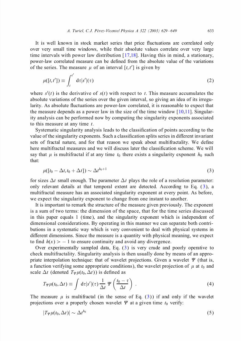
Fig. 1. Ten-year daily series of the log of prices for TelefÃonica (TEF).

2. Settings

We have processed two dierent kind of data belonging to the Spanish stock market

(IBEX) which correspond to well dierent time scales. The ÿrst group is formed by

daily series of 17 dierent assets (those with the largest liquidity) during approximately

ten years (from January 1st, 1990 to May 24th, 2001) containing 48458 points. The

second group consists of 12 month series (during 1999) for the 4 most important

assets of the market, also included in Euro Stoxx 50, each series being sampled at atime interval of one minute containing 275477 points. For this group, there are clear,

systematic disruptions at precise moments such as the opening of the local market or

the opening of NY market (3:30 p.m. local hour), for instance. In spite of the fact

that those events elicit statistical deviations from the multifractal model, they do not

aect signiÿcantly to our calculations due to the high sampling rate. For that reason

we do not try to correct the systematic deviations by any mean, performing the same

analysis for the two groups. In the same spirit, we always identify the ending of a

session as the instant just preceding the opening of the following, no matter the actual

time interval between them (sometimes several non-working days) for both types of

series. Examples of series of the two types are shown in Figs. 1 and 2.We are interested in relative variations of the price, i.e., the ratio of the absolute

value to the absolute variation. For that reason, we will work on series formed by

logarithms of prices. In such a way, the absolute variation between two consecutive

instants (approximately, the derivative with respect to time) for this series approximates

the relative variation for the original stock series.

3. Multifractal analysis

3.1. Singularity analysis

Self-similar (or multifractal) signals are usually characterized by a very irregular

behaviour: at some point they show very abrupt transitions while in points nearby the




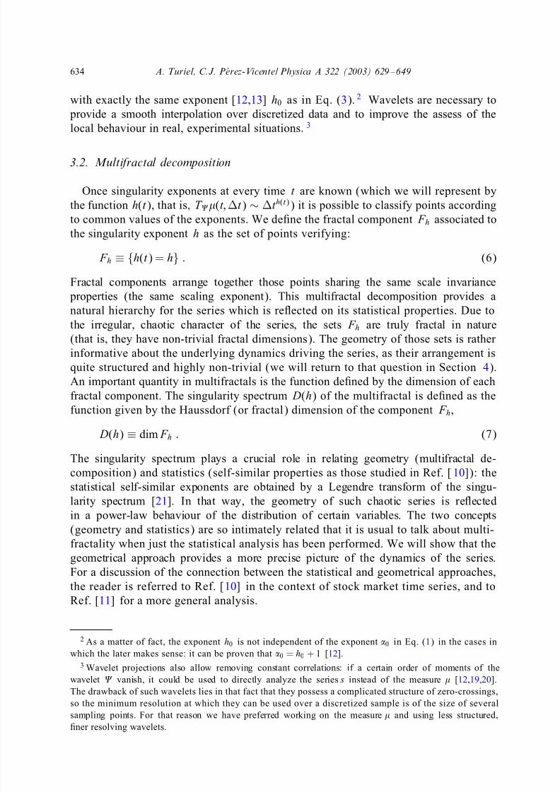
Fig. 2. November 1999 minute series of the log of prices for TelefÃonica (TEF).

function behaves rather smoothly. Such systems are also scale invariant, what means

that no statistical variable can depend on an inner scale: the process should seem

the same when a change in scale is performed. Combining both principles (irregular

distribution of transitions, scale invariance) it should be expected that the series s(t )

can be expanded around a given instant t 0 as:

| s(t ) − s(t 0)| ∼ |t − t 0|0 : (1)

The exponent 0 is the so called singularity exponent or Holder exponent [13] associ-

ated to t 0. Eq. (1) is of course scale invariant, and the smooth or irregular character of

the transition at t 0 depends on value of 0. The greater the exponent, the most regular

the signal will be at that point.

It is expected that the value of the singularity exponents associated to the dierent

instants vary greatly, in order to give account of the irregular nature of the series. To

describe the series, it would be then convenient to calculate the singularity exponents

at every time t , that is, to perform a singularity analysis of the series. The naif way

to proceed is to test Eq. (1) at every time t 0 and to calculate the function (t 0)of singularity exponents. Singularity analysis thus generalizes the concept of Taylor

expansion for irregular, chaotic signals.

Such a simple singularity analysis is rather standard in the study of turbulent ows,

and it has been used in dierent studies of stock market series as well as in Ref. [10].

However that deÿnition of singularity exponent (Eq. (1)) is not well adapted for signals

with constant contributions to the two-point correlation. This is the case for intermittent,

locally non-stationary signals, in which uctuations are long lived [14]. In that case, the

lack of stationarity masks the presence of positive singularity exponents, making them

impossible to detect. There are two possibilities to overcome this diculty: to build a

stationary measure (as in Ref. [15]) or to project the signal over a wavelet basis (asin Ref. [16]). We will apply both techniques: the ÿrst, to create a stationary signal;

the second, to provide a smooth way to interpolate data over discretized sampling.




It is well known in stock market series that price uctuations are correlated only

over very small time windows, while their absolute values correlate over very large

time intervals with power law distribution [17,18]. Having this in mind, a stationary,

power-law correlated measure can be deÿned from the absolute value of the variationsof the series. The measure of an interval [t; t ] is given by

([t; t ]) ≡

t

t

d| s|() (2)

where s(t ) is the derivative of s(t ) with respect to t . This measure accumulates the

absolute variations of the series over the given interval, so giving an idea of its irregu-

larity. As absolute uctuations are power-law correlated, it is reasonable to expect that

the measure depends as a power law in the size of the time window [10,11]. Singular-

ity analysis can be performed now by computing the singularity exponents associatedto this measure at any time t .

Systematic singularity analysis leads to the classiÿcation of points according to the

value of the singularity exponents. Such a classiÿcation splits series in dierent invariant

sets of fractal nature, and for that reason we speak about multifractality. We deÿne

here multifractal measures and we will discuss later the classiÿcation scheme. We will

say that is multifractal if at any time t 0 there exists a singularity exponent h0 such

that:

([t 0 − t; t 0 + t ]) ∼ t h0+1 (3)

for sizes t small enough. The parameter t plays the role of a resolution parameter:only relevant details at that temporal extent are detected. According to Eq. (3), a

multifractal measure has an associated singularity exponent at every point. As before,

we expect the singularity exponent to change from one instant to another.

It is important to remark the structure of the measure given previously. The exponent

is a sum of two terms: the dimension of the space, that for the time series discussed

in this paper equals 1 (time), and the singularity exponent which is independent of

dimensional considerations. By operating in this manner we can separate both contri-

butions in a systematic way which is very convenient to deal with physical systems in

dierent dimensions. Since the measure is a quantity with physical meaning, we expect

to ÿnd h( x) ¿ − 1 to ensure continuity and avoid any divergence.

Over experimentally sampled data, Eq. (3) is very crude and poorly operative to

check multifractality. Singularity analysis is then usually done by means of an appro-

priate interpolation technique: that of wavelet projections. Given a wavelet (that is,

a function verifying some appropriate conditions), the wavelet projection of at t 0 and

scale t (denoted T (t 0; t )) is deÿned as

T (t 0; t ) ≡

d| s|()

1

t

t 0 −

t

: (4)

The measure is multifractal (in the sense of Eq. (3)) if and only if the wavelet projections over a properly chosen wavelet at a given time t 0 verify:

|T (t 0; t )| ∼ t h0 (5)




with exactly the same exponent [12,13] h0 as in Eq. (3). 2 Wavelets are necessary to

provide a smooth interpolation over discretized data and to improve the assess of the

local behaviour in real, experimental situations. 3

3.2. Multifractal decomposition

Once singularity exponents at every time t are known (which we will represent by

the function h(t ), that is, T (t; t ) ∼ t h(t )) it is possible to classify points according

to common values of the exponents. We deÿne the fractal component F h associated to

the singularity exponent h as the set of points verifying:

F h ≡ {h(t ) = h} : (6)

Fractal components arrange together those points sharing the same scale invariance

properties (the same scaling exponent). This multifractal decomposition provides a

natural hierarchy for the series which is reected on its statistical properties. Due to

the irregular, chaotic character of the series, the sets F h are truly fractal in nature

(that is, they have non-trivial fractal dimensions). The geometry of those sets is rather

informative about the underlying dynamics driving the series, as their arrangement is

quite structured and highly non-trivial (we will return to that question in Section 4).

An important quantity in multifractals is the function deÿned by the dimension of each

fractal component. The singularity spectrum D(h) of the multifractal is deÿned as the

function given by the Haussdorf (or fractal) dimension of the component F h

,

D(h) ≡ dim F h : (7)

The singularity spectrum plays a crucial role in relating geometry (multifractal de-

composition) and statistics (self-similar properties as those studied in Ref. [ 10]): the

statistical self-similar exponents are obtained by a Legendre transform of the singu-

larity spectrum [21]. In that way, the geometry of such chaotic series is reected

in a power-law behaviour of the distribution of certain variables. The two concepts

(geometry and statistics) are so intimately related that it is usual to talk about multi-

fractality when just the statistical analysis has been performed. We will show that the

geometrical approach provides a more precise picture of the dynamics of the series.For a discussion of the connection between the statistical and geometrical approaches,

the reader is referred to Ref. [10] in the context of stock market time series, and to

Ref. [11] for a more general analysis.

2 As a matter of fact, the exponent h0 is not independent of the exponent 0 in Eq. (1) in the cases in

which the later makes sense: it can be proven that 0 = h0 + 1 [12].3 Wavelet projections also allow removing constant correlations: if a certain order of moments of the

wavelet vanish, it could be used to directly analyze the series s instead of the measure [12,19,20].

The drawback of such wavelets lies in that fact that they possess a complicated structure of zero-crossings,so the minimum resolution at which they can be used over a discretized sample is of the size of several

sampling points. For that reason we have preferred working on the measure and using less structured,

ÿner resolving wavelets.




Fig. 3. Function h(t ) for TelefÃonica daily series (Fig. 1). It is strongly irregular. Theory predicts that it is

everywhere discontinuous [12], what is connected with the fact that its level sets (the fractal components)

are of non-trivial fractal dimensions. The total discontinuity of h(t ) makes the fractal components to be

strongly spatially correlated (randomly placed singularities would lead to some continuity points). For that

reason, contrary to intuition multifractal series are quite structured.

3.3. Experimental results

All the series were analyzed using several wavelets from the Laplacian family,(t ) = (1 + t 2)−, with = 1; 1:5; 2. Such functions are not admissible wavelets,

that is, they cannot be used to represent any particular series [ 13]; they can be used

however to perform singularity analysis on positive multifractal measures [12]. Those

particular wavelets provide a ÿne spatial localization at the cost of restricting the range

of singularities which is possible to detect. Those functions are able to resolve all the

eective range of singularities in log-Poisson multifractals, which is the case of the

analyzed series (we will discuss log-Poisson multifractals in Section 4). The exponent

h(t ) at every time t was computed as the slope of a log-log linear regression of the

absolute value of the wavelet projection vs. the resolution t (see Eq. (5)), for reso-

lutions continuously sampled in the interval [1; 3] (here the units are tics, i.e., number of points). In all the stock market series, for a vast majority of the points (¿ 99%)

the linear regression exhibited good regression coecient (absolute value above 0.9),

validating the multifractal framework. For details on wavelet singularity analysis the

reader is referred to Ref. [12] and references therein.

The results obtained with the dierent wavelets are comparable. In Fig. 3 we show

a typical exponent function h(t ); as it is clearly seen, it is extremely irregular, chaotic

in behaviour. It is thus not so surprising that the dierent fractal components are

truly fractal in character. We had not tried to provide a representation of each fractal

component, as they have a very complicated structure, dicult to decipher from a

simple plot.The experimental distribution of singularities showed that the possible values for the

singularity exponents were in all the cases contained in a range included in [ −1; 2] (see




Fig. 4. Experimental distribution of h for TelefÃonica daily series.

Fig. 4). There always existed a non-trivial, minimum value h∞ verifying −1 ¡ h∞ ¡ 0,

as we expected. The existence of a ÿnite lower bound in h is not surprising: the range

of possible singularities is always bounded from below for ÿnite variation series (that

is, the series can be discontinuous, but not too sharply; see Ref. [12] for a discussion).

The range of singularities is not a priori bounded from above however, but in the

experimental results it turned out to be so.

3.4. Log-normal vs. log-Poisson statistics

The observed distribution of singularity exponents ÿts the log-Poisson model; on the

contrary, it is incompatible with the log-normal model. Why? Because in the log-normal

model the singularity exponents h are not bounded, neither from above nor from below.

In Fig. 5 we show a typical log-normal series. It was generated using the model pre-

sented in Ref. [22], and the parameters were chosen to have a regular power spectrum

and a reasonable dispersion. As it can be observed in Fig. 5, log-normal series have

sudden bursts which are extremely singular, but at the same time they are rather scarce(they correspond to events in the negative tail of the distribution of singularities). It

is clear however from simple visual inspection that such a series does not resemble a

real one due precisely to those unbounded bursts. The frequency of them is controlled

by the dispersion of the gaussian, but they will eventually happen for a large enough

data set.

This discrepancy with the behaviour of real series is also evidenced when the

series is analyzed using the geometrical approach. In Fig. 6 we present the distribution

of singularity exponents associated to the log-normal series in Fig. 5. It assigns a

non-null probability to extremely negative singularity exponents (which correspond to

the bursts), which is physically unreasonable but characteristic of an unbounded dis-tribution of singularities as the log-normal one. In contrast, singularities in real data

are bounded, in agreement with the log-Poisson model. This boundness does not mean




Fig. 5. A typical log-normal series. It was generated using the model in Ref. [22]. The coecients ÿt a

log-normal of log-mean 0, and log-dispersion 0.5. The series contains 16384 points, and the basis wavelet

is the second derivative of the gaussian.

Fig. 6. Experimental distribution of h for the log normal series represented in Fig. 5.

that the series is bounded (it could grow forever, for instance), but that there is no

jump to inÿnity at any point.

However, multifractal stock series are quite often described in the scientiÿc litera-

ture using log-normal statistics (for instance, in Ref. [23]). In such works the authors

estimate the statistical self-similarity exponents from the data and make a quadratic ÿt

(which corresponds to log-normal statistics) for some low-order moments. Finer analy-

sis, as the one shown in Ref. [10], show a considerable deviation from the log-normal

model for larger moments (which are precisely the ones dominated by the most sin-

gular exponents). What actually happens is that log-Poisson is indeed approximatedin law by a log-normal as a consequence of Central Limit Theorem when the scale

change is large enough. But as this approximation is granted in law, just the most




probable events are approximately equally distributed as in a log-normal model, while

rare events (and specially the most singular events) are poorly described. Depending

on the application, a log-normal model could be a good approximation or a very poor

one. We will see in the following that in a geometrical picture it is precisely thoserare events which allow to describe the whole series, and for that reason log-normal

models are of no use in our context.

4. MSM and reconstruction

4.1. Theoretical background

Log-Poisson models are characterized by a very simple statistical feature: when aninÿnitesimally small change of scale takes place, just two events can happen: either the

random variable changes smoothly or it undergoes a sudden change. The last possibility

is interpreted as the crossing of one particular fractal component which concentrates

the energy dissipation (in the case of turbulent ows) of the multifractal. A complete

discussion about the statistics of log-Poisson multifractals and its interpretations would

be quite extensive and somewhat pointless to be carried out here; the reader is referred

to the wide bibliography on the subject. Let us cite here the basic works introducing

the model and discussing its properties for turbulent ows [24 – 27]. For a discus-

sion of the interplay between statistics and geometry and the relevance of log-Poisson

statistics for multifractal decomposition, we refer to Ref. [12], in which the main ques-tions are reviewed in a quite dierent context of application (the statistics of natural

images).

According to Ref. [12], in log-Poisson multifractals there is a particular fractal com-

ponent of maximum information content, the so called Most Singular Manifold (MSM).

Log-Poisson statistics of changes in scale are characterized by the event of crossing

or not that particular set. The MSM is deÿned as the fractal component associated

to the least possible exponent h∞ (that as we have seen veriÿes −1 ¡ h∞ ¡ 0 for

ÿnite variation signals). We will denote shortly the MSM by F ∞ ≡ F h∞ . Due to the

statistical interpretation of the MSM, in Ref. [28] it was proposed that a multifractal

signal could be reconstructed from the values of the gradient over the MSM; as anhypothesis, it was stated that reconstruction is performed by means of a linear kernel.

The kernel was uniquely determined under several reasonable requirements (isotropy,

translational invariance and correspondence with the experimental power spectrum).

We do not present here the whole derivation but the ÿnal expression; the reader is

referred to the original paper. We will make use of the ÿnal formula to generalize it

to the context of 1D series.

Let us start by deÿning the essential data needed to reconstruct. We will consider

now a multifractal signal s deÿned over a multidimensional space, the points being

identiÿed by their vector coordinates x. Hence, the signal will be given by the function

s(x). The multifractal measure is deÿned as the integral of |∇ s|(x), the modulus of the gradient, over the measured sets. The test of multifractality and singularity detection

are carried out analogously to what was done for 1D signals. Let us deÿne the essential




gradient ÿeld,

v(x) ≡ ∇ s(x) F ∞ (x) ; (8)

where F ∞ (x) is a delta-like function constant over the MSM F ∞ and vanishing outsidethat set. So, ˜ v contains all the information (geometry of the MSM and value of the

measure over it) which we need to reconstruct, according to what is discussed in

Ref. [28]. As it is shown in that reference, the signal can be reconstructed using the

following formula (expressed in the Fourier space):

ˆ s(˜ f) = i˜ f · ˆ v(˜ f)

f2; (9)

where hat (ˆ) denotes Fourier transform, ˜ f is the frequency variable in the Fourier

domain, i is the imaginary unit and the symbol “ · ” means scalar product of vectors.Let us notice that this formula has an interesting stability property: if we choose as

F ∞ the total space, then v = ∇ s, that is, ˆv(˜ f) = −i˜ f ˆ s(˜ f); substituting in Eq. (9) we

see that the equality is trivially satisÿed. This means that there always exists a set

(in the worst case, the whole space) from which reconstruction is perfect. A signal is

reconstructible if there exists a smaller, rather sparse set F ∞ from which reconstruction

is possible; or conversely, points not in F ∞ are predictable from those in F ∞.

The 1=f2 factor in Eq. (9) creates a diusion eect for signals in dimensions

greater than 1, as this is the Fourier representation of a Green function associated

to the Laplacian operator. A strong simpliÿcation appears when Eq. (9) is applied to

one-dimensional signals; then it reduces to:

ˆ s(f) = iv(f)

f: (10)

But i=f is a representation of the indeÿnite integral, 4 that is, an inverse of the deriva-

tive (as ˆ s(f) = −if ˆ s(f)). So the reconstruction formula in 1D becomes:

s(t ) = s(0) +

t

0

d v() : (11)

Let us make a few remarks on this formula. First, it has obviously the aforementioned

stability property: if F ∞ is taken as the whole interval the formula is a trivial identity,as v(t ) becomes s(t ) in such a case. Also, recalling that v(t ) = s(t ) F ∞(t ) we see

that the weight of this function is concentrated in point-like contributions, in the points

belonging to the MSM. For that reason, the series s(t ) obtained according to Eq. (11)

is piecewise constant, undergoing a change on its value when a point of the MSM is

crossed.

Secondly, let us notice that Eq. (11) does not imply that s(t ) = 0 for t ∈ F ∞. For

continuous, ideal series, F ∞ is a dense set; therefore at any time t and any size there

4 In the original derivation, the signal s had zero-mean to avoid divergence at zero frequency in Eq. (9);

for that reason the ambiguity in the choice of the constant is removed. In principle we assume that theintegral of s over the considered time window is zero, what eliminates the ambiguity in the choice of the

indeÿnite integral. We can change the convention to determine this constant, keeping consistency; in fact

we have done it in Eq. (11) by adding the term s(0).




are points belonging to the MSM in (t − ; t + ), and so t +

t −d v() is non-vanishing

in general. It follows that the derivative of the series s(t ) given in Eq. (11) can be

dierent from zero even at t ∈ F ∞.

On the contrary, over real, discretized data there is necessarily a loss in resolution:the integral in Eq. (11) becomes a sum and the derivative is turned into the subtraction

of consecutive values; hence, the only points which can be removed in the sequence are

those for which s(t ) = 0 strictly. However, at a given level of detail some points may

be discarded without causing a great deviation between the reconstructed series and the

real one. These points are obviously those for which the derivative is very small, but

also other points in which the variations (derivatives) are signiÿcant but immediately

compensated by changes of the opposite sign and similar absolute value. The key

point is not the absolute value of the variations, but the resolution at which the series

is described: signiÿcant variations are those which are large enough in comparison

with those of the points nearby. At a given resolution, there will be an optimal set

consisting of the points with the most signiÿcant changes. In fact, it is logical that the

MSM could be identiÿed with that set: it contains the points with the most negative

exponents, that is, the points over which the transition (variation) is the sharpest. For

those points the derivative is signiÿcantly greater than over the surrounding points (we

will see in the following that the reconstruction out the MSM is rather good).

Determining the MSM is a rather standard procedure, much better than trying to

assess by other means which points could be discarded when reconstructing. Calcu-

lating singularity exponents allows classifying the points according to the strength of

the transition the series undergoes at them, giving a reasonable criterion to includeor discard points in the MSM at a given precision, depending on the uncertainty or

dispersion on the value h∞. We will then use the MSM as minimum reconstructing

set.

4.2. Experimental results and discussion

In Fig. 7 we represent the reconstructed series for one daily and one minute sampling

series; other series threw very similar results. In each case the MSM was determined via

wavelet analysis as explained in Section 3; the MSMs were chosen as h∞=−0:40±0:3

(daily series) and h∞ = −0:45 ± 0:3 (minute series). The central value of h∞ wasdetermined as the average of the points associated to the 1% and the 5% left tails of

the probability distribution of singularities h, as in Ref. [12]. The uncertainty range

(±0:3) was conventionally ÿxed in such a way that the quality of the reconstruction

was reasonable enough. As it is seen in Fig. 7 the quality of the reconstruction is very

good. According to Eq. (11), the ÿrst point in the series has zero error and starting from

it the error accumulates as time passes; for that reason the last point in the series is

necessarily the worst predicted (in average). It is reasonable to proceed in such a way,

as we deal with time series and one of the goals of this study is to make predictions

and uctuation estimation. Notice that the shape of the series is well captured by the

reconstructed estimates, and errors mainly accumulate during very sharp transitions(specially for the periodic disruptions in minute series) which probably constitute a

deviation from the multifractal description and should be treated separately. In spite




Fig. 7. Original (+) and reconstructed (×) (out the MSM) series for the daily series of TelefÃonica (left;

PSNR for the reconstructed series: 27:86 dB) and for the 1-min series (right; PSNR: 24 :64 dB).

Fig. 8. Original (+) and reconstructed (×) (out a uniform sampling) series for TelefÃonica: daily (left; PSNR:

14:24 dB) and 1-min (right; PSNR: 12:03 dB).

of the presence of disruptive points in minute series, the reconstructed series provides

good approximation. This is due to the fact that during a short period after a disruptive

event (for instance, opening of NY market) the variations are larger than typical, but

they keep however the same multifractal arrangement, the MSM being still predictive.

Just the very ÿrst instants fail to be described in the multifractal picture, and they are

quite few. For that reason the present description is still valid in a good extent.For the chosen quantization in h∞ (±0:3), the density ∞ of the MSM was always

rather high (∞ = 0:30 for the daily series, ∞ = 0:29 for the minute series). It could

seem that the high quality of the reconstruction is just a consequence of the high value

of the density for the MSM; however, if we replace the MSM in the reconstruction

formula by uniform or random samplings with the same density, the quality is much

lower (see Figs. 8 and 9). This fact shows that the MSM has a large information

content. Besides, the series obtained for those non-structured samplings have not a

well deÿned tendency (they are not clearly, or not as much as the original series,

increasing or decreasing). This implies that positive and negative variations are almost

equally likely in price series: they are continuously oscillating. But, what is moresurprising, the distributions of absolute values for positive and negative increments are

quite similar. How to explain the tendency in the series?




Fig. 9. Original (+) and reconstructed (×) (out a random sampling) series for TelefÃonica: daily (left; PSNR:

12:09 dB) and 1-min (right; PSNR: 10:50 dB).

Tendency changes just take place over the MSM, which is quite reduced in com-

parison to the total amount of points. Over the MSM, the distributions of positive and

negative increments are still quite similar. However, the amount of positive increments

is greater (vs. smaller) than that of the negative ones for increasing (vs. decreasing)

series; they are of the same order for no tendency series. For that reason, what de-

termines the tendency of the series is not the absolute values of its increments, but

the dierence in number of positive and negative increments over the MSM. It is now

obvious that tendency is dicult to assess with a sampling independent of the MSM.

For instance, a random or uniform sampling of the whole series at 0.30 density would

just sample 30% of MSM points, giving rise to a series with 30% as much tendency

as the original one. To end the discussion, just remark that the characterization of the

MSM as the set of tendency points is another way to express that MSM points are

the most singular, the most signiÿcant with respect to their surroundings. Points out-

side the MSM are surrounded by similar, opposed tendency points, giving rise to a

vanishing change in tendency.

We have shown that the MSM plays a fundamental role in the dynamics of the

temporal series; ideally the series is fully described using this skeleton, this essential

set. According to the reconstruction formula, Eq. (11), and the deÿnition of the essential

gradient, Eq. (8) (for 1D in our case), there are two dierent types of information whichare needed to reconstruct, namely the geometry of the MSM (given by F ∞(t )) and

the values of the derivative s on MSM. In the next section we will try to describe the

dynamics governing the geometrical arrangement of the MSM; we leave the study of

the intensities of the derivatives for a future work.

5. Dynamics on the MSM

Let us ÿrst deÿne the MSM oriented density function, o F ∞

(t ), which is given by:

o F ∞

(t ) =

F ∞

(t ) if t ∈ F ∞; s(t ) ¿ 0 ;

− F ∞(t ) if t ∈ F ∞; s(t ) ¡ 0 ;

0 if t ∈ F ∞ :

(12)




So the oriented density function keeps the sign of the derivative on the MSM. This

function keeps the information about the geometry of the MSM (as |0 F ∞

| = F ∞), and

at the same time it already incorporates some basic information about the derivative

(its sign). This sign weighting is necessary to allow the possibility of cancellationswhen resolution is changed. Besides, as it was discussed in the previous section, the

proportion of signs determines the tendency of the series. 5 In some sense, the function

o F ∞

deÿnes a naif series in which every event (non-zero value) means a relative change

in the price of shares of the same absolute value. For that reason, a good understanding

of the dynamics of this function could be useful to device a naif sell-buy model capable

to produce correct multifractal exponents (that is, the statistics of changes in scale).

For this analysis, we took averages over the two ensembles of data, assuming mutual

statistical consistency among the dierent series they consisted of.

We tried ÿrst to identify two-point dependencies in o

F ∞. We computed the mutual

information between o F ∞

(t ) and o F ∞

(t + ) for dierent time delays ; assuming sta-

tionary statistics we disregard the basis points t . The generic value of o F ∞

(t ) at any

point will be denoted by , which can take the values −1, 1 or 0, depending if t

belongs to the MSM with negative derivative, if t belongs to the MSM with positive

derivative, or if t does not belong to the MSM, respectively. We adopt the following

convention: a subscript associated to a state (i.e., ) indicates that the state takes

place at a point which is displaced units with respect to a generic base point. We

calculated the two-point joint probability as

P (0; ) = Prob(o F ∞

(t ) = 0; o F ∞

(t + ) = )t (13)

and the marginal probability as

P () =

Prob(o F ∞

(t ) = )

t = P (; )

for any : (14)

The mutual information between the points of the oriented MSM I is then given by

I =

0=−1;0;1

=−1;0;1

P (0; )log2

P (0; )

P (0) P ()(15)

that is, the Kullback distance between the joint probability P (0; ) and the product of

the marginal probabilities P (0) P () [29]; it is expressed in bits. It equals the entropy

when the two variables are identical and vanishes only when they are independent; for

that reason it is a good measure of statistical dependency. In Fig. 10 we present the

graphs of I for both ensembles.

Results for both ensembles are comparable. The mutual information I decays

extremely fast with the time displacement , so that at three time units of distance

it is already negligible (comparable with the sampling uncertainty). This means that

points in the MSM separated by such a distance can be considered independent. We

would like to provide a stationary random process able to describe correctly this

behaviour.

5 In fact the oriented density possesses stronger features: it deÿnes (via the reconstruction formula) a

multifractal series with the same singularity exponents as the original series. Its analysis will deserve future

works.




Fig. 10. Mutual information I in semi-log plot for daily ensemble (continuous line) and 1-min ensemble

(dashed).

We propose that the joint probability P (0; ) is obtained by successive appli-

cations of an elementary transition matrix T on P (0) (in fact this means that the

random process is a Markov chain). In this model long range dependencies are a con-

sequence of successive one-unit dependencies. Let us use P (0; 2) as an example. We

can express it as

P (0; 2) = P (2|0) P (0) ; (16)

where P (|0) stands for the conditional probability of obtaining the state at the

point at units of distance once the state at the base point is ÿxed to 0. Let us expand

the conditional probability in terms of the intermediate state 1; we obtain:

P (0; 2) =

1

P (2; 1|0) P (0) : (17)

Conditioning with respect to 1 it is obtained:

P (0; 2) =

1 P (2|1; 0) P (1|0) P (0) : (18)

We assume that the random process is a stationary Markov chain, what means

P (2|1; 0) = P (2|1). Applying it to the previous expression:

P (0; 2) =

1

P (2|1) P (1|0) P (0) (19)

and comparing with Eq. (16) we obtain the ÿnal formula for the random process:

P (2|0) = 1

P (2|1) P (1|0) (20)

that is, P (2|0) is obtained by two applications of the random process described by

P (1|0). Let us introduce a matricial notation. We will represent the random process




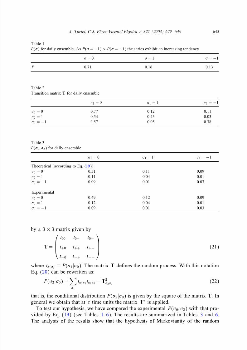
Table 1

P () for daily ensemble. As P ( = +1) ¿ P ( =−1) the series exhibit an increasing tendency

= 0 = 1 =−1

P 0.71 0.16 0.13

Table 2

Transition matrix T for daily ensemble

1 = 0 1 = 1 1 =−1

0 = 0 0.77 0.12 0.11

0 = 1 0.54 0.43 0.03

0 =−1 0.57 0.05 0.38

Table 3

P (0 ; 2) for daily ensemble

1 = 0 1 = 1 1 =−1

Theoretical (according to Eq. (19))

0 = 0 0.51 0.11 0.09

0 = 1 0.11 0.04 0.01

0 =−1 0.09 0.01 0.03

Experimental

0 = 0 0.49 0.12 0.09

0 = 1 0.12 0.04 0.01

0 =−1 0.09 0.01 0.03

by a 3 × 3 matrix given by

T =

t 00 t 0+ t 0−

t +0 t ++ t +−

t −0 t −+ t −−

(21)

where t 10≡ P (1|0). The matrix T deÿnes the random process. With this notation

Eq. (20) can be rewritten as:

P (2|0) =

1

t 21t 10

= T220

(22)

that is, the conditional distribution P (2|0) is given by the square of the matrix T. In

general we obtain that at time units the matrix T is applied.

To test our hypothesis, we have compared the experimental P (0; 2) with that pro-vided by Eq. (19) (see Tables 1 – 6). The results are summarized in Tables 3 and 6.

The analysis of the results show that the hypothesis of Markovianity of the random




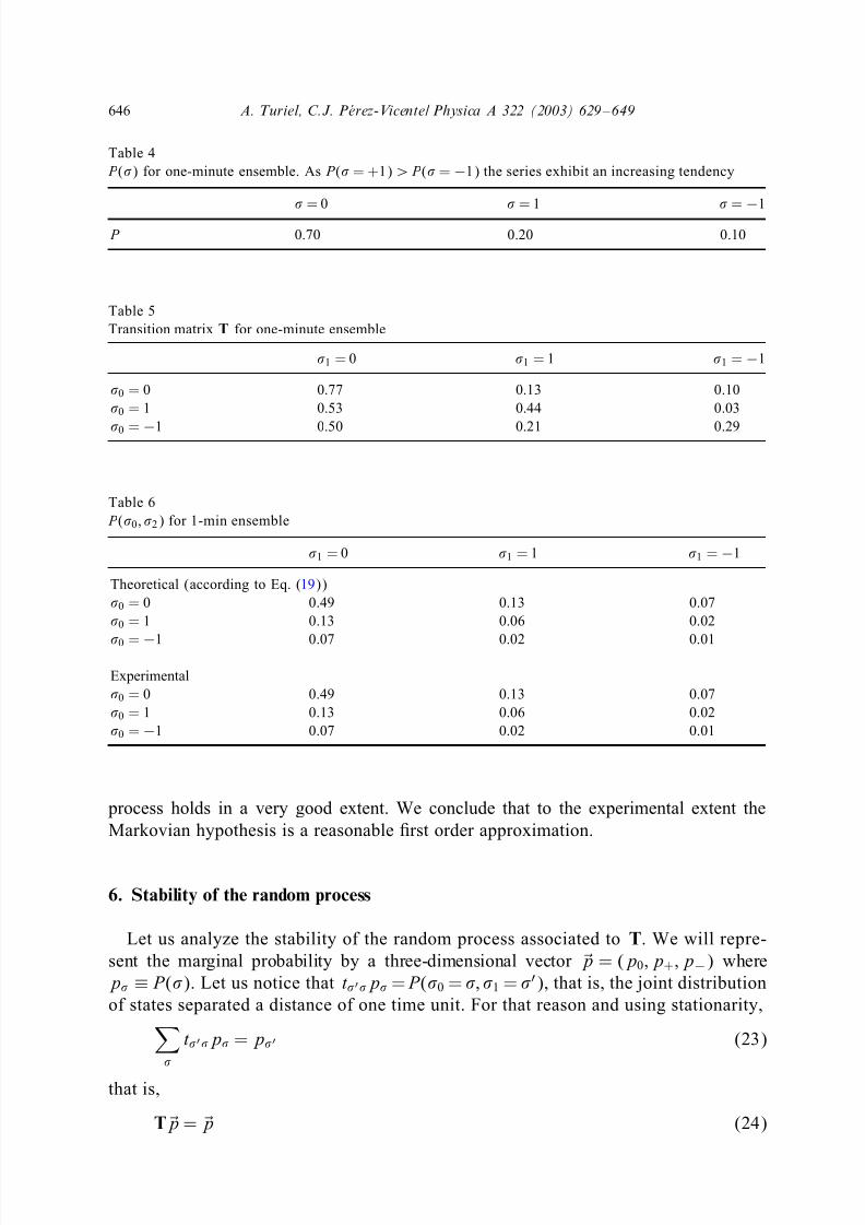
Table 4

P () for one-minute ensemble. As P ( = +1) ¿ P ( =−1) the series exhibit an increasing tendency

= 0 = 1 =−1

P 0.70 0.20 0.10

Table 5

Transition matrix T for one-minute ensemble

1 = 0 1 = 1 1 =−1

0 = 0 0.77 0.13 0.10

0 = 1 0.53 0.44 0.03

0 =−1 0.50 0.21 0.29

Table 6

P (0 ; 2) for 1-min ensemble

1 = 0 1 = 1 1 =−1

Theoretical (according to Eq. (19))

0 = 0 0.49 0.13 0.07

0 = 1 0.13 0.06 0.02

0 =−1 0.07 0.02 0.01

Experimental

0 = 0 0.49 0.13 0.07

0 = 1 0.13 0.06 0.02

0 =−1 0.07 0.02 0.01

process holds in a very good extent. We conclude that to the experimental extent the

Markovian hypothesis is a reasonable ÿrst order approximation.

6. Stability of the random process

Let us analyze the stability of the random process associated to T. We will repre-

sent the marginal probability by a three-dimensional vector ˜ p = (p0; p+; p−) where

p ≡ P (). Let us notice that t p = P (0 = ; 1 = ), that is, the joint distribution

of states separated a distance of one time unit. For that reason and using stationarity,

t p = p (23)

that is,

T˜ p = ˜ p (24)




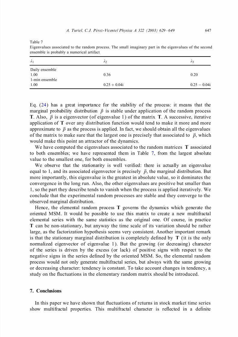
Table 7

Eigenvalues associated to the random process. The small imaginary part in the eigenvalues of the second

ensemble is probably a numerical artifact

1 2 3

Daily ensemble

1.00 0.36 0.20

1-min ensemble

1.00 0:25 + 0:04i 0:25− 0:04i

Eq. (24) has a great importance for the stability of the process: it means that the

marginal probability distribution ˜ p is stable under application of the random process

T. Also, ˜ p is a eigenvector (of eigenvalue 1) of the matrix T. A successive, iterativeapplication of T over any distribution function would tend to make it more and more

approximate to ˜ p as the process is applied. In fact, we should obtain all the eigenvalues

of the matrix to make sure that the largest one is precisely that associated to ˜ p, which

would make this point an attractor of the dynamics.

We have computed the eigenvalues associated to the random matrices T associated

to both ensembles; we have represented them in Table 7, from the largest absolute

value to the smallest one, for both ensembles.

We observe that the stationarity is well veriÿed: there is actually an eigenvalue

equal to 1, and its associated eigenvector is precisely ˜ p, the marginal distribution. But

more importantly, this eigenvalue is the greatest in absolute value, so it dominates theconvergence in the long run. Also, the other eigenvalues are positive but smaller than

1, so the part they describe tends to vanish when the process is applied iteratively. We

conclude that the experimental random processes are stable and they converge to the

observed marginal distribution.

Hence, the elemental random process T governs the dynamics which generate the

oriented MSM. It would be possible to use this matrix to create a new multifractal

elemental series with the same statistics as the original one. Of course, in practice

T can be non-stationary, but anyway the time scale of its variation should be rather

large, as the factorization hypothesis seems very consistent. Another important remark

is that the stationary marginal distribution is completely deÿned by T (it is the onlynormalized eigenvector of eigenvalue 1). But the growing (or decreasing) character

of the series is driven by the excess (or lack) of positive signs with respect to the

negative signs in the series deÿned by the oriented MSM. So, the elemental random

process would not only generate multifractal series, but always with the same growing

or decreasing character: tendency is constant. To take account changes in tendency, a

study on the uctuations in the elementary random matrix should be introduced.

7. Conclusions

In this paper we have shown that uctuations of returns in stock market time series

show multifractal properties. This multifractal character is reected in a deÿnite




geometry for the series, arranged around fractal components of characteristic power

law behaviour under changes in scale. We have exploited further this geometry and we

have experimentally shown that the most singular of the fractal components (that is, the

one which is dominant when the scale is reduced) can be used to reconstruct the wholeseries to a good extent. This means that the information about the series is contained

in this set and its dynamics is driven by it. It has a highly non-trivial structure (what

questions claims of “lack of structure” for economics series), as can be seen for the

poor performance of random and uniform sampling with the same density. Also, an

important information about the dynamics generating the MSM can be deduced from

the data: at least in a good ÿrst order approximation, this set is constructed as a result

of a Markov chain random process, in which the state of the point (which characterizes

if the point belongs to the MSM, and its orientation in this case) is only dependent on

the state of the previous point. This random process could be considered as the basis

event to describe the dynamics underlying the series.

Future directions that should be addressed concerns the stability and econometric

interpretation of this elemental random process, as its performance in generating good

multifractal series, even prediction. A dierent but important issue to be considered is

the description of the actual intensity (gradient) proÿle on the MSM. In fact, it can

be proven (as it will be shown in future works) that it follows a slow varying pattern

with however very important events.

Acknowledgements

A. Turiel is ÿnancially supported by a postdoctoral grant from the INRIA. We thank

GÃerard Weisbusch and specially Jean-Pierre Nadal for their help and support in the

elaboration of this work and their comments. We also thank Sociedad de Bolsas as

well as Risklab-Madrid for providing the data and Mcyt (contract BFM2000-0626) for

ÿnancial support.

References

[1] J.P. Bouchaud, M. Potters, Theory of Financial Risk, Cambridge University Press, Cambridge, 2000.

[2] R.N. Mantegna, H.E. Stanley, An introduction to Econophysics, Cambridge University Press, Cambridge,

1999.

[3] R.N. Mantegna, H.E. Stanley, Scaling behavior of an economic index, Nature 376 (1995) 46–49.

[4] S. Galluccio, G. Caldarelli, M. Marsili, Y.-C. Zhang, Scaling in currency exchange, Physica A 245

(1997) 423–436.

[5] B.B. Mandelbrot, The variation of certain speculative prices, Journal of Bussiness XXXVI (1963)

392–417.

[6] B. Mandelbrot, H.M. Taylor, On the distribution of stock price dierences, Oper. Res. 15 (1967)

1057–1062.

[7] R.N. Mantegna, H. Stanley, Turbulence and ÿnancial markets, Nature 376 (1996) 46–49.

[8] S. Ghashghaie, W. Breymann, J. Peinke, P. Talkner, Y. Dodge, Turbulent cascades in foreign exchangemarket, Nature 381 (1996) 767.

[9] F. Schmitt, D. Schertzer, S. Lovejoy, Multifractal uctuations in ÿnance, Int. J. Theoret. Appl. Finance

3 (2000) 361–364.




[10] Y. Fujiwara, H. Fujisaka, Coarse-graining and self-similarity of price uctuations, Physica A 294 (2001)

439.

[11] A. Arneodo, Wavelet analysis of fractals: from the mathematical concepts to experimental reality, in:

G. Erlebacher, M.Y. Hussaini, L. Jameson (Eds.), Wavelets. Theory and applications, ICASE/LaRCSeries in Computational Science and Engineering, Oxford University Press, Oxford, 1996, p. 349.

[12] A. Turiel, N. Parga, The multi-fractal structure of contrast changes in natural images: from sharp edges

to textures, Neural Comput. 12 (2000) 763–793.

[13] I. Daubechies, Ten lectures on wavelets, CBMS-NSF Series in Applied Mathematics, Capital City Press,

Montpelier, Vermont, 1992.

[14] A. Davis, A. Marshak, W. Wiscombe, Wavelet based multifractal analysis of non-stationary and/or

intermittent geophysical signals, in: E. Foufoula-Georgiou, P. Kumar (Eds.), Wavelet Transforms in

Geophysics, Academic Press, New York, 1994, pp. 249–298.

[15] B.B. Mandelbrot, A. Fisher, L. Calvet, A multifractal model of asset returns, Cowles Foundation

Discussion Paper No. 1164.

[16] A. Arneodo, J.-F. Muzy, D. Sornette, “direct” causal cascade in the stock market, Eur. Phys. J. B 2

(1998) 277–282.[17] Y. Liu, P. Gopikrishnan, P. Cizeau, M. Meyer, C.-K. Peng, H.E. Stanley, The statistical properties of

the volatility of price uctuations, Phys. Rev. E 60 (1999) 1390–1400.

[18] P. Gopikrishnan, V. Plerou, Y. Liu, L.A.N. Amaral, X. Gabaix, H.E. Stanley, Scaling and correlation

in ÿnancial time series, Physica A 287 (2000) 362–373.

[19] A. Arneodo, F. Argoul, E. Bacry, J. Elezgaray, J.F. Muzy, Ondelettes, multifractales et turbulence,

Diderot Editeur, Paris, France, 1995.

[20] A. Turiel, N. Parga, Multifractal wavelet ÿlter of natural images, Phys. Rev. Lett. 85 (2000) 3325–

3328.

[21] G. Parisi, U. Frisch, On the singularity structure of fully developed turbulence, in: M. Ghil, R. Benzi,

G. Parisi (Eds.), Turbulence and Predictability in Geophysical Fluid Dynamics, Proceedings of the

International School of Physics E. Fermi, North Holland, Amsterdam, 1985, pp. 84–87.

[22] R. Benzi, L. Biferale, A. Crisanti, G. Paladin, M. Vergassola, A. Vulpiani, A random process for the

construction of multiane ÿelds, Physica D 65 (1993) 352–358.

[23] J.F. Muzy, J. Delour, E. Bacry, Modelling uctuations of ÿnancial time series: from cascade process to

stochastic volatility model, Euro. Phys. J. B 17 (2000) 537–548.

[24] B. Dubrulle, Intermittency in fully developed turbulence: Log-poisson statistics and generalized scale

covariance, Phys. Rev. Lett. 73 (1994) 959–962.

[25] Z.S. She, E. Leveque, Universal scaling laws in fully developed turbulence, Phys. Rev. Lett. 72 (1994)

336–339.

[26] Z.S. She, E.C. Waymire, Quantized energy cascade and log-poisson statistics in fully developed

turbulence, Phys. Rev. Lett. 74 (1995) 262–265.

[27] B. Castaing, The temperature of turbulent ows, J. Phys. II 6 (1996) 105–114.

[28] A. Turiel, A. del Pozo, Reconstructing images from their most singular fractal manifold, IEEE Trans.Im. Proc. 11 (2002) 345–350.

[29] T.M. Cover, J.A. Thomas, Elements of Information Theory, John Wiley, New York, 1991.

finance - multifractal geometry - turiel perez-vicente 2003

Documents