introduction to algorithms - dspace@mit:...
TRANSCRIPT
Introduction to Algorithms6.046J/18.401J/SMA5503
Lecture 23Prof. Charles E. Leiserson
Introduction to Algorithms Day 40 L23.2© 2001 by Charles E. Leiserson© 2001 by Charles E. Leiserson
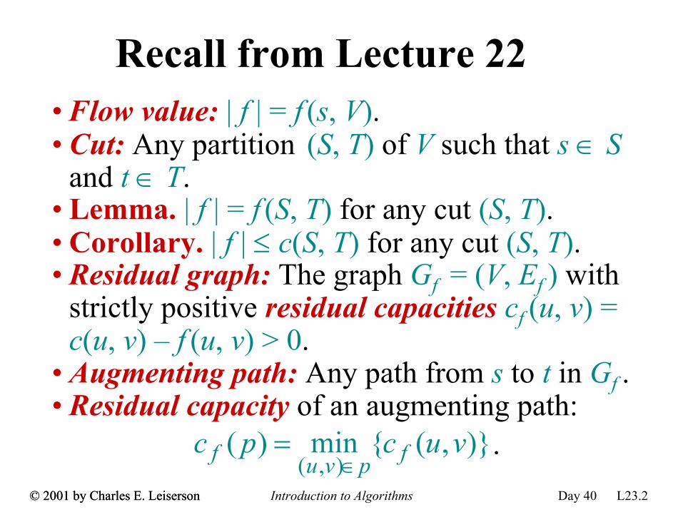
Recall from Lecture 22• Flow value: | f | = f (s, V).• Cut: Any partition (S, T) of V such that s ∈ S
and t ∈ T.• Lemma. | f | = f (S, T) for any cut (S, T). • Corollary. | f | ≤ c(S, T) for any cut (S, T).• Residual graph: The graph Gf = (V, Ef ) with
strictly positive residual capacities cf (u, v) = c(u, v) – f (u, v) > 0.
• Augmenting path: Any path from s to t in Gf .• Residual capacity of an augmenting path:
)},({min)(),(
vucpc fpvuf ∈= .
Introduction to Algorithms Day 40 L23.3© 2001 by Charles E. Leiserson© 2001 by Charles E. Leiserson
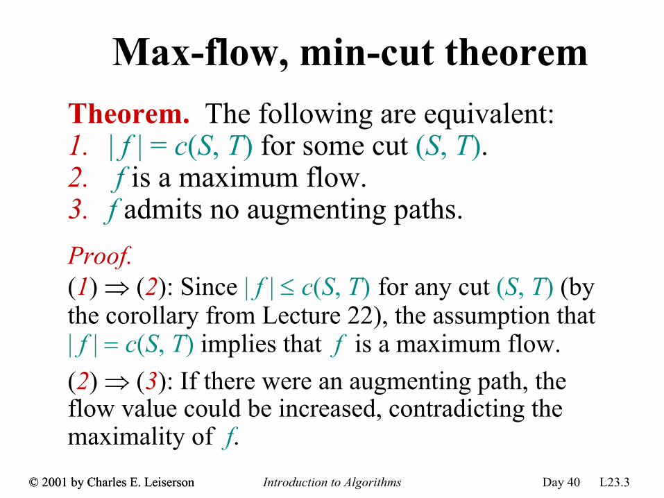
Max-flow, min-cut theoremTheorem. The following are equivalent:1. | f | = c(S, T) for some cut (S, T).2. f is a maximum flow.3. f admits no augmenting paths.Proof. (1) ⇒ (2): Since | f | ≤ c(S, T) for any cut (S, T) (by the corollary from Lecture 22), the assumption that | f | = c(S, T) implies that f is a maximum flow.(2) ⇒ (3): If there were an augmenting path, the flow value could be increased, contradicting the maximality of f.
Introduction to Algorithms Day 40 L23.4© 2001 by Charles E. Leiserson© 2001 by Charles E. Leiserson
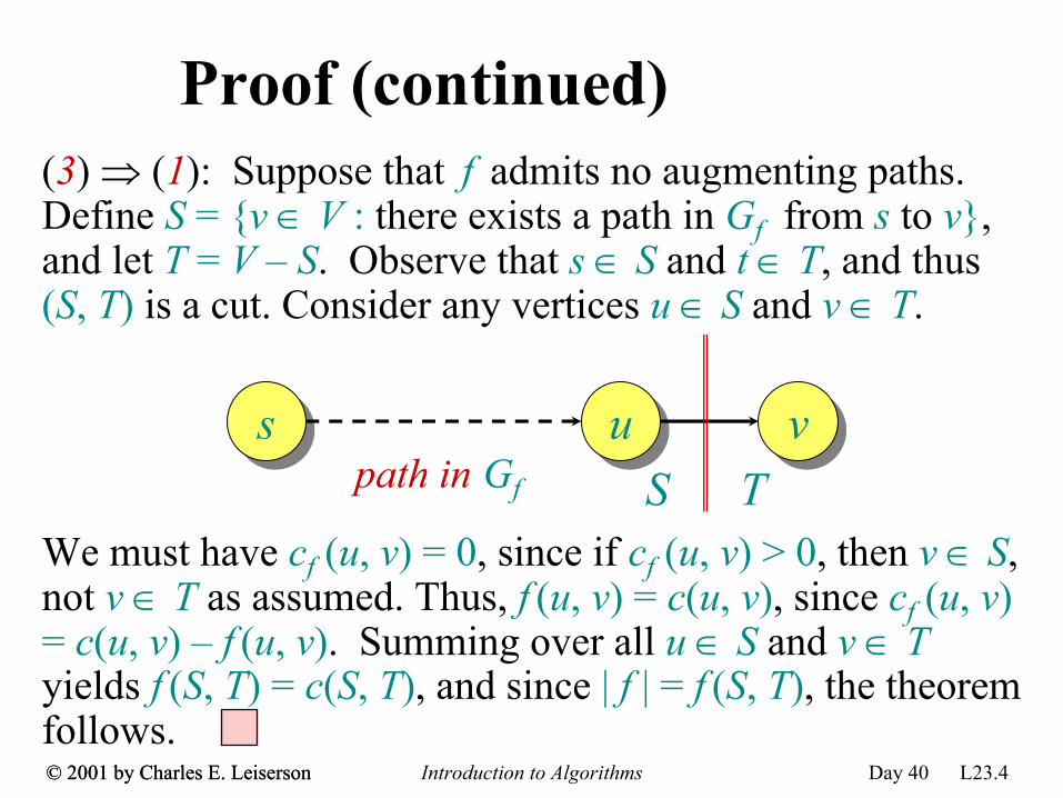
Proof (continued)(3) ⇒ (1): Suppose that f admits no augmenting paths. Define S = {v ∈ V : there exists a path in Gf from s to v}, and let T = V – S. Observe that s ∈ S and t ∈ T, and thus (S, T) is a cut. Consider any vertices u ∈ S and v ∈ T.
We must have cf (u, v) = 0, since if cf (u, v) > 0, then v ∈ S, not v ∈ T as assumed. Thus, f (u, v) = c(u, v), since cf (u, v) = c(u, v) – f (u, v). Summing over all u ∈ S and v ∈ Tyields f (S, T) = c(S, T), and since | f | = f (S, T), the theorem follows.
ss uu vvS Tpath in Gf
Introduction to Algorithms Day 40 L23.5© 2001 by Charles E. Leiserson© 2001 by Charles E. Leiserson
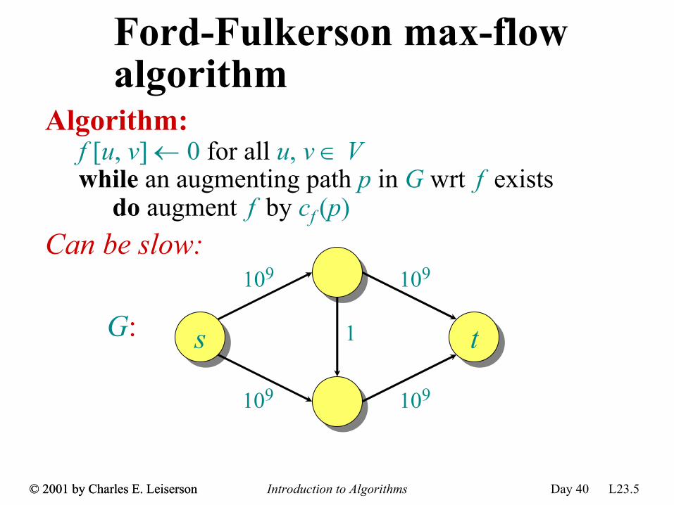
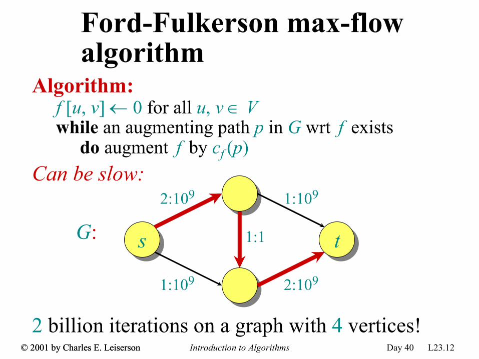
Ford-Fulkerson max-flow algorithm
Algorithm:f [u, v] ← 0 for all u, v ∈ Vwhile an augmenting path p in G wrt f exists
do augment f by cf (p)Can be slow:
ss tt
109 109
109
1
109
G:
Introduction to Algorithms Day 40 L23.6© 2001 by Charles E. Leiserson© 2001 by Charles E. Leiserson
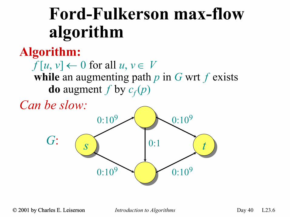
Ford-Fulkerson max-flow algorithm
Can be slow:
ss tt
0:109 0:109
0:109
0:1
0:109
G:
Algorithm:f [u, v] ← 0 for all u, v ∈ Vwhile an augmenting path p in G wrt f exists
do augment f by cf (p)

Introduction to Algorithms Day 40 L23.7© 2001 by Charles E. Leiserson© 2001 by Charles E. Leiserson
Ford-Fulkerson max-flow algorithm
Can be slow:
ss tt
0:109 0:109
0:109
0:1
0:109
G:
Algorithm:f [u, v] ← 0 for all u, v ∈ Vwhile an augmenting path p in G wrt f exists
do augment f by cf (p)

Introduction to Algorithms Day 40 L23.8© 2001 by Charles E. Leiserson© 2001 by Charles E. Leiserson
Ford-Fulkerson max-flow algorithm
Can be slow:
ss tt
1:109 0:109
1:109
1:1
0:109
G:
Algorithm:f [u, v] ← 0 for all u, v ∈ Vwhile an augmenting path p in G wrt f exists
do augment f by cf (p)
Introduction to Algorithms Day 40 L23.9© 2001 by Charles E. Leiserson© 2001 by Charles E. Leiserson
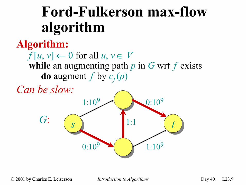
Ford-Fulkerson max-flow algorithm
Can be slow:
ss tt
1:109 0:109
1:109
1:1
0:109
G:
Algorithm:f [u, v] ← 0 for all u, v ∈ Vwhile an augmenting path p in G wrt f exists
do augment f by cf (p)

Introduction to Algorithms Day 40 L23.10© 2001 by Charles E. Leiserson© 2001 by Charles E. Leiserson
Ford-Fulkerson max-flow algorithm
Can be slow:
ss tt
1:109 1:109
1:109
0:1
1:109
G:
Algorithm:f [u, v] ← 0 for all u, v ∈ Vwhile an augmenting path p in G wrt f exists
do augment f by cf (p)
Introduction to Algorithms Day 40 L23.11© 2001 by Charles E. Leiserson© 2001 by Charles E. Leiserson
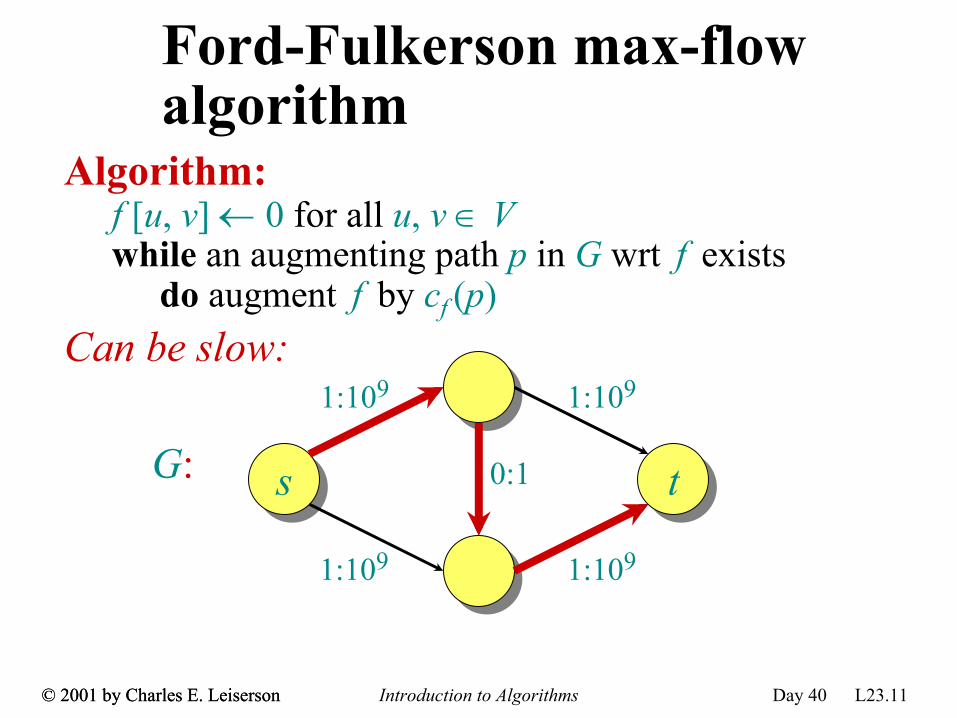
Ford-Fulkerson max-flow algorithm
Can be slow:
ss tt
1:109 1:109
1:109
0:1
1:109
G:
Algorithm:f [u, v] ← 0 for all u, v ∈ Vwhile an augmenting path p in G wrt f exists
do augment f by cf (p)
Introduction to Algorithms Day 40 L23.12© 2001 by Charles E. Leiserson© 2001 by Charles E. Leiserson
Ford-Fulkerson max-flow algorithm
Can be slow:
ss tt
2:109 1:109
2:109
1:1
1:109
G:
2 billion iterations on a graph with 4 vertices!
Algorithm:f [u, v] ← 0 for all u, v ∈ Vwhile an augmenting path p in G wrt f exists
do augment f by cf (p)
Introduction to Algorithms Day 40 L23.13© 2001 by Charles E. Leiserson© 2001 by Charles E. Leiserson
Edmonds-Karp algorithmEdmonds and Karp noticed that many people’s implementations of Ford-Fulkerson augment along a breadth-first augmenting path: a shortest path in Gf from s to t where each edge has weight 1. These implementations would always run relatively fast.Since a breadth-first augmenting path can be found in O(E) time, their analysis, which provided the first polynomial-time bound on maximum flow, focuses on bounding the number of flow augmentations.(In independent work, Dinic also gave polynomial-time bounds.)

Introduction to Algorithms Day 40 L23.14© 2001 by Charles E. Leiserson© 2001 by Charles E. Leiserson
Monotonicity lemmaLemma. Let δ(v) = δf (s, v) be the breadth-first distance from s to v in Gf . During the Edmonds-Karp algorithm, δ(v) increases monotonically.Proof. Suppose that f is a flow on G, and augmentation produces a new flow f ′. Let δ′(v) = δf ′(s, v). We’ll show that δ′(v) ≥ δ(v) by induction on δ(v). For the base case, δ′(s) = δ(s) = 0.For the inductive case, consider a breadth-first path s →L → u → v in Gf ′. We must have δ′(v) = δ′(u) + 1, since subpaths of shortest paths are shortest paths. Certainly, (u, v) ∈ Ef ′ , and now consider two cases depending on whether (u, v) ∈ Ef .
Introduction to Algorithms Day 40 L23.15© 2001 by Charles E. Leiserson© 2001 by Charles E. Leiserson
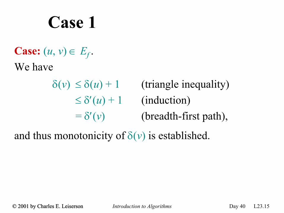
Case 1Case: (u, v) ∈ Ef .
δ(v) ≤ δ(u) + 1 (triangle inequality)≤ δ′(u) + 1 (induction)= δ′(v) (breadth-first path),
and thus monotonicity of δ(v) is established.
We have
Introduction to Algorithms Day 40 L23.16© 2001 by Charles E. Leiserson© 2001 by Charles E. Leiserson
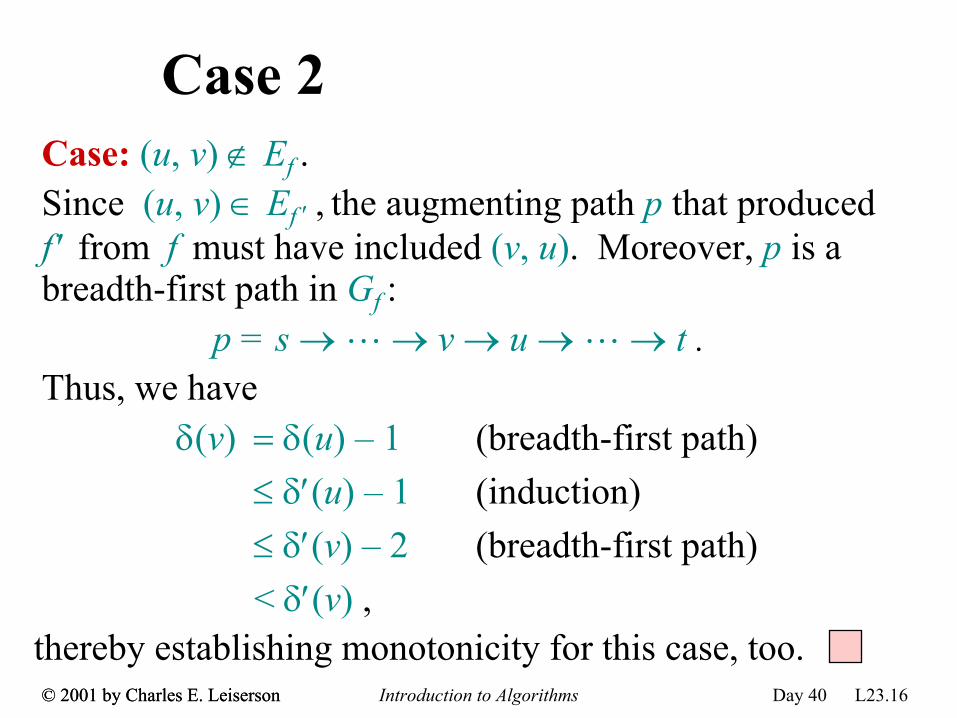
Case 2Case: (u, v) ∉ Ef .Since (u, v) ∈ Ef ′ , the augmenting path p that produced f ′ from f must have included (v, u). Moreover, p is a breadth-first path in Gf :
p = s → L → v → u → L → t .Thus, we have
δ(v) = δ(u) – 1 (breadth-first path)≤ δ′(u) – 1 (induction)≤ δ′(v) – 2 (breadth-first path)< δ′(v) ,
thereby establishing monotonicity for this case, too.
Introduction to Algorithms Day 40 L23.17© 2001 by Charles E. Leiserson© 2001 by Charles E. Leiserson
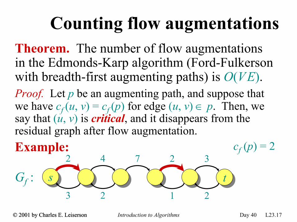
Counting flow augmentationsTheorem. The number of flow augmentations in the Edmonds-Karp algorithm (Ford-Fulkerson with breadth-first augmenting paths) is O(VE).Proof. Let p be an augmenting path, and suppose that we have cf (u, v) = cf (p) for edge (u, v) ∈ p. Then, we say that (u, v) is critical, and it disappears from the residual graph after flow augmentation.
ss
2
3
Gf :4
2
7 2
1tt
3cf (p) = 2Example:
2
Introduction to Algorithms Day 40 L23.18© 2001 by Charles E. Leiserson© 2001 by Charles E. Leiserson
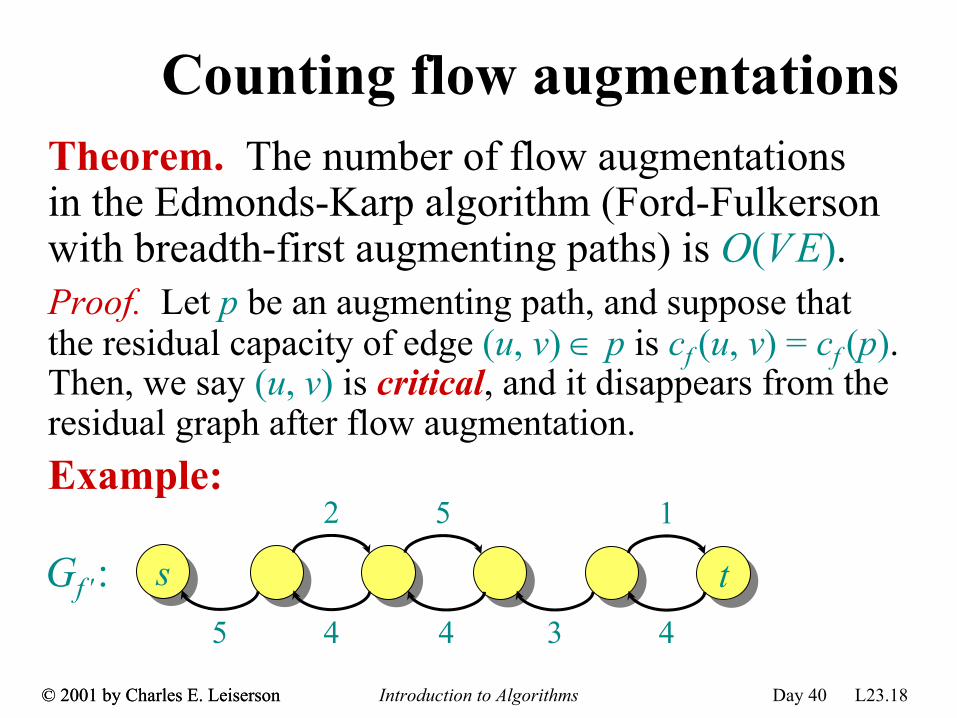
Counting flow augmentationsTheorem. The number of flow augmentations in the Edmonds-Karp algorithm (Ford-Fulkerson with breadth-first augmenting paths) is O(VE).Proof. Let p be an augmenting path, and suppose that the residual capacity of edge (u, v) ∈ p is cf (u, v) = cf (p). Then, we say (u, v) is critical, and it disappears from the residual graph after flow augmentation.
ss5
Gf ′:2
4
5
3tt
1Example:
4 4
Introduction to Algorithms Day 40 L23.19© 2001 by Charles E. Leiserson© 2001 by Charles E. Leiserson
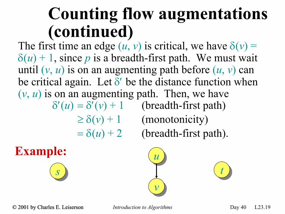
Counting flow augmentations (continued)
The first time an edge (u, v) is critical, we have δ(v) = δ(u) + 1, since p is a breadth-first path. We must wait until (v, u) is on an augmenting path before (u, v) can be critical again. Let δ′ be the distance function when (v, u) is on an augmenting path. Then, we have
ssuu
vvtt
Example:
δ′(u) = δ′(v) + 1 (breadth-first path)≥ δ(v) + 1 (monotonicity)= δ(u) + 2 (breadth-first path).
Introduction to Algorithms Day 40 L23.20© 2001 by Charles E. Leiserson© 2001 by Charles E. Leiserson
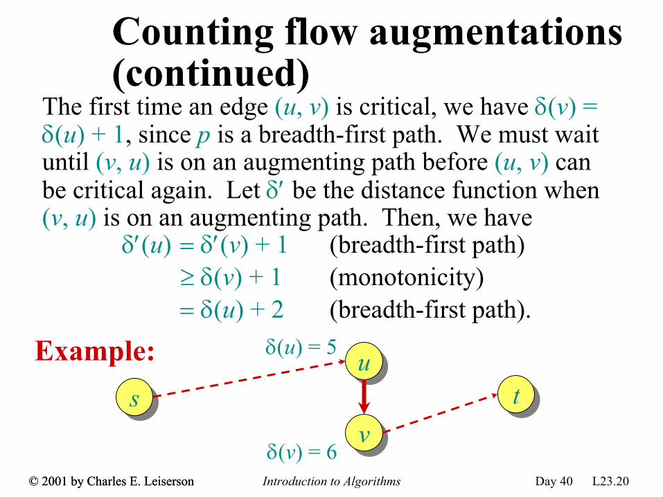
Counting flow augmentations (continued)
The first time an edge (u, v) is critical, we have δ(v) = δ(u) + 1, since p is a breadth-first path. We must wait until (v, u) is on an augmenting path before (u, v) can be critical again. Let δ′ be the distance function when (v, u) is on an augmenting path. Then, we have
δ′(u) = δ′(v) + 1 (breadth-first path)≥ δ(v) + 1 (monotonicity)= δ(u) + 2 (breadth-first path).
ssuu
vvtt
δ(u) = 5
δ(v) = 6
Example:
Introduction to Algorithms Day 40 L23.21© 2001 by Charles E. Leiserson© 2001 by Charles E. Leiserson
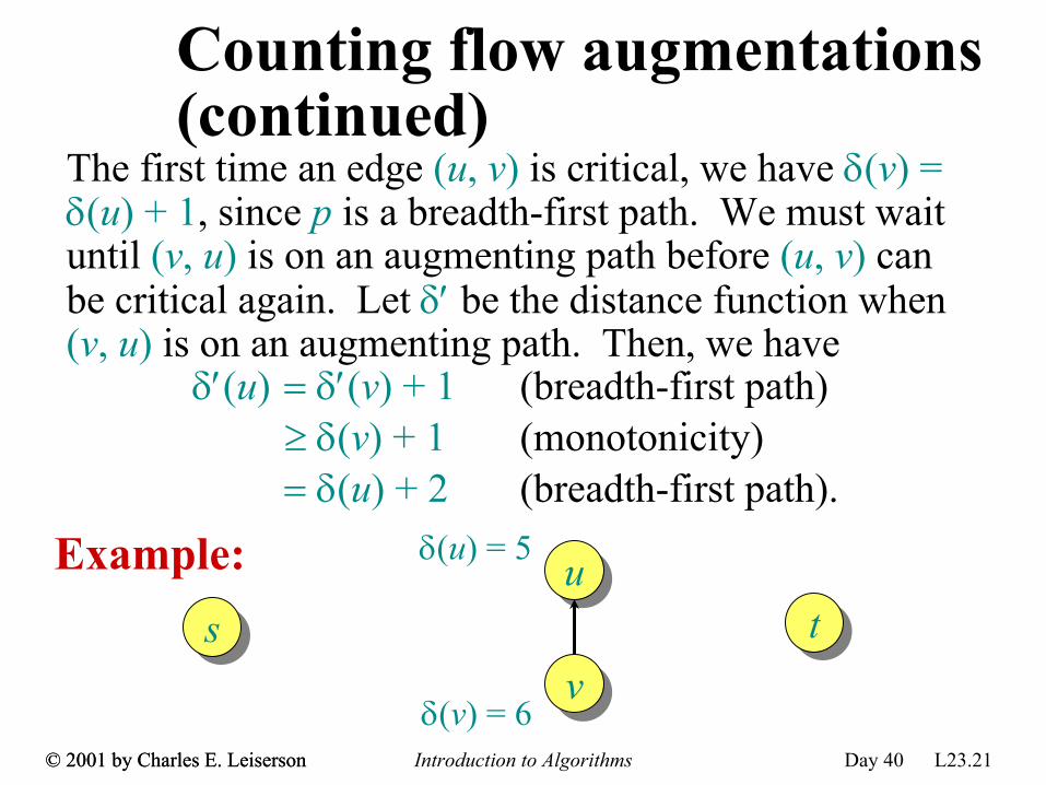
Counting flow augmentations (continued)
The first time an edge (u, v) is critical, we have δ(v) = δ(u) + 1, since p is a breadth-first path. We must wait until (v, u) is on an augmenting path before (u, v) can be critical again. Let δ′ be the distance function when (v, u) is on an augmenting path. Then, we have
ssuu
vvtt
δ(u) = 5
δ(v) = 6
Example:
δ′(u) = δ′(v) + 1 (breadth-first path)≥ δ(v) + 1 (monotonicity)= δ(u) + 2 (breadth-first path).
Introduction to Algorithms Day 40 L23.22© 2001 by Charles E. Leiserson© 2001 by Charles E. Leiserson
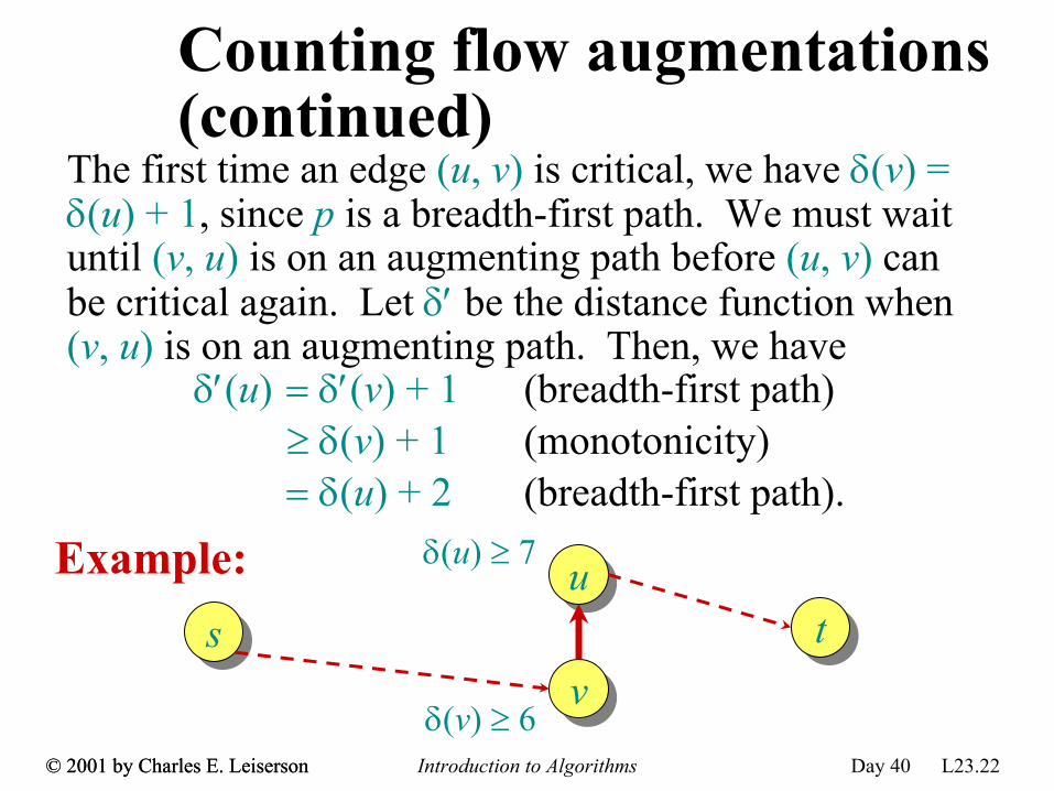
Counting flow augmentations (continued)
The first time an edge (u, v) is critical, we have δ(v) = δ(u) + 1, since p is a breadth-first path. We must wait until (v, u) is on an augmenting path before (u, v) can be critical again. Let δ′ be the distance function when (v, u) is on an augmenting path. Then, we have
ssuu
vvtt
δ(u) ≥ 7
δ(v) ≥ 6
Example:
δ′(u) = δ′(v) + 1 (breadth-first path)≥ δ(v) + 1 (monotonicity)= δ(u) + 2 (breadth-first path).

Introduction to Algorithms Day 40 L23.23© 2001 by Charles E. Leiserson© 2001 by Charles E. Leiserson
Counting flow augmentations (continued)
The first time an edge (u, v) is critical, we have δ(v) = δ(u) + 1, since p is a breadth-first path. We must wait until (v, u) is on an augmenting path before (u, v) can be critical again. Let δ′ be the distance function when (v, u) is on an augmenting path. Then, we have
ssuu
vvtt
δ(u) ≥ 7
δ(v) ≥ 6
Example:
δ′(u) = δ′(v) + 1 (breadth-first path)≥ δ(v) + 1 (monotonicity)= δ(u) + 2 (breadth-first path).

Introduction to Algorithms Day 40 L23.24© 2001 by Charles E. Leiserson© 2001 by Charles E. Leiserson
Counting flow augmentations (continued)
The first time an edge (u, v) is critical, we have δ(v) = δ(u) + 1, since p is a breadth-first path. We must wait until (v, u) is on an augmenting path before (u, v) can be critical again. Let δ′ be the distance function when (v, u) is on an augmenting path. Then, we have
ssuu
vvtt
δ(u) ≥ 7
δ(v) ≥ 8
Example:
δ′(u) = δ′(v) + 1 (breadth-first path)≥ δ(v) + 1 (monotonicity)= δ(u) + 2 (breadth-first path).
Introduction to Algorithms Day 40 L23.25© 2001 by Charles E. Leiserson© 2001 by Charles E. Leiserson
Running time of Edmonds-Karp
Distances start out nonnegative, never decrease, and are at most |V| – 1 until the vertex becomes unreachable. Thus, (u, v) occurs as a critical edge O(V) times, because δ(v) increases by at least 2 between occurrences. Since the residual graph contains O(E) edges, the number of flow augmentations is O(V E).
Corollary. The Edmonds-Karp maximum-flow algorithm runs in O(V E2) time.Proof. Breadth-first search runs in O(E) time, and all other bookkeeping is O(V) per augmentation.
Introduction to Algorithms Day 40 L23.26© 2001 by Charles E. Leiserson© 2001 by Charles E. Leiserson
Best to date• The asymptotically fastest algorithm to date for
maximum flow, due to King, Rao, and Tarjan, runs in O(V E logE/(V lg V)V) time.
• If we allow running times as a function of edge weights, the fastest algorithm for maximum flow, due to Goldberg and Rao, runs in time
O(min{V 2/3, E1/2} ⋅ E lg (V 2/E + 2) ⋅ lg C),where C is the maximum capacity of any edge in the graph.