branching algorithms - inria · branching algorithms are also called i branch & bound...

Branching Algorithms

Dieter Kratsch

Laboratoire d’Informatique Theorique et AppliqueeUniversite Paul Verlaine - Metz

57000 Metz Cedex 01France

AGAPE 09, Corsica, FranceMay 24 - 29, 2009

1/122

I. Our First Independent Set Algorithm:

mis1

2/122

Independent Set

Definition (Independent Set)

Let G = (V ,E ) be a graph. A subset I ⊆ V of vertices of G is anindependent set of G if no two vertices in I are adjacent.

Definition (Maximum Independent Set (MIS))

Given a graph G = (V ,E ), compute the maximum cardinality ofan independent set of G , denoted by α(G ).

[or a maximum independent set of G ]

a

b

c

d e

f

3/122

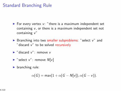
Standard Branching Rule

I For every vertex v : ”there is a maximum independent setcontaining v , or there is a maximum independent set notcontaining v”

I Branching into two smaller subproblems: ”select v” and”discard v” to be solved recursively

I ”discard v”: remove v

I ”select v”: remove N[v ]

I branching rule:

α(G ) = max(1 + α(G − N[v ]), α(G − v)).

4/122

Algorithm mis1

int mis1(G = (V ,E ));

if (∆(G ) ≥ 3) choose any vertex v of degree d(v) ≥ 3

return max(1 + mis1(G − N[v ]),mis1(G − v));

if (∆(G ) ≤ 2) compute α(G ) in polynomial time

and return the value;

5/122

Intro Branch & Recharge Lower bounds Sort & Search

The branching rule

The branching rule is really simple. Given a vertex v on which wewant to branch :! “select v” and recursively build all (!, ")-DS containing v! “discard v” and recursively build all (!, ")-DS not containing v

v

v !

select v

v !

discard v

(!, ")-DScontaining v

(!, ")-DSnot containing v

13/406/122

Correctness

I standard branching rule correct; hence branching does notmiss any maximum independent set

I graphs of maximum degree two are disjoint union of pathsand cycles

I α(G ) easy to compute if ∆(G ) ≤ 2 [exercice]

I mis1 outputs α(G ) for input graph G

I mis1 can be modified s.t. it outputs a maximum independentset

7/122

Time Analysis via recurrence

I Running time of mis1 is O∗(T (n)), where

I T (n) is largest number of base cases for any input graph G onn vertices

I Base case = graph of maximum degree two for which α iscomputed by a polynomial time algorithm

I branching rule implies recurrence:

T (n) ≤ T (n − 1) + T (n − d(v)− 1) ≤ T (n − 1) + T (n − 4)

8/122

Solving the Recurrence

I Solutions of recurrence of form cn

I Basic solutions root of characteristic polynomial

xn = xn−1 + xn−4

I largest root of characteristic polynomial is its unique positivereal root

I Maple, Mathematica, Matlab etc.

9/122

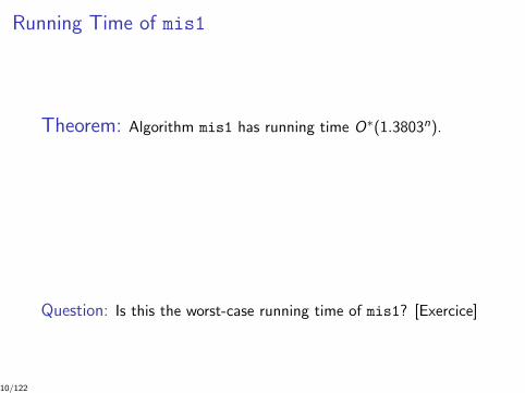
Running Time of mis1

Theorem: Algorithm mis1 has running time O∗(1.3803n).

Question: Is this the worst-case running time of mis1? [Exercice]

10/122

II. Fundamental Notions and Time Analysis

11/122

Branching Algorithms

are also called

I branch & bound algorithms

I backtracking algorithms

I search tree algorithms

I branch & reduce algorithms

I splitting algorithms

The technique is also called ”Pruning the search tree”

(e.g. in Woeginger’s well-known survey).

12/122

Branching and Reduction Rules

Branching algorithms are recursively applied to instances of aproblem using branching rules and reduction rules.

I Branching rules: solve a problem instance by recursivelysolving smaller instances

I Reduction rules:

- simplify the instance- (typically) reduce the size of the instance

13/122

Search Trees

I Search Tree:

used to illustrate, understand and analyse an execution of abranching algorithm

I root: assign the input to the root

I node: assign to each node a solved problem instance

I child: each instance reached by a branching rule is assigned toa child of the node of the original instance of the problem

14/122

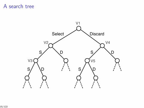
A search tree

Select Discard

S

S S

S D

D

D

D

V1

V2 V4

V3 V5

15/122

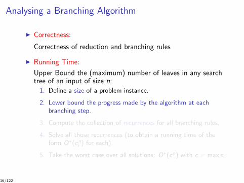
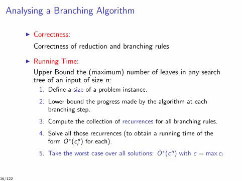
Analysing a Branching Algorithm

I Correctness:

Correctness of reduction and branching rules

I Running Time:

Upper Bound the (maximum) number of leaves in any searchtree of an input of size n:

1. Define a size of a problem instance.

2. Lower bound the progress made by the algorithm at eachbranching step.

3. Compute the collection of recurrences for all branching rules.

4. Solve all those recurrences (to obtain a running time of theform O∗(cn

i ) for each).

5. Take the worst case over all solutions: O∗(cn) with c = max ci

16/122

Simple Time Analysis : Search Tree

I Assumption: for any node of search tree polynomial runningtime.

I Time analysis of branching algorithms means to upper boundthe number of nodes of any search tree of an input of size n.

I Let T (n) be (an upper bound of) the maximum number ofleaves of any search tree of an input of size n.

I Running time of corresponding branching algorithm:O∗(T (n))

I Branching rules to be analysed separately

17/122

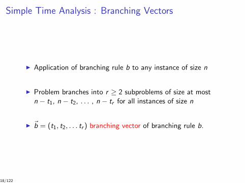
Simple Time Analysis : Branching Vectors

I Application of branching rule b to any instance of size n

I Problem branches into r ≥ 2 subproblems of size at mostn − t1, n − t2, . . . , n − tr for all instances of size n

I ~b = (t1, t2, . . . tr ) branching vector of branching rule b.

18/122

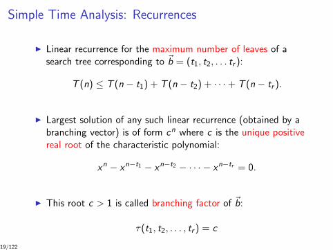
Simple Time Analysis: Recurrences

I Linear recurrence for the maximum number of leaves of asearch tree corresponding to ~b = (t1, t2, . . . tr ):

T (n) ≤ T (n − t1) + T (n − t2) + · · ·+ T (n − tr ).

I Largest solution of any such linear recurrence (obtained by abranching vector) is of form cn where c is the unique positivereal root of the characteristic polynomial:

xn − xn−t1 − xn−t2 − · · · − xn−tr = 0.

I This root c > 1 is called branching factor of ~b:

τ(t1, t2, . . . , tr ) = c

19/122

Properties of Branching Vectors [Kullmann]

Let r ≥ 2. Let ti > 0 for all i ∈ 1, 2, . . . r.

1. τ(t1, t2, . . . , tr ) ∈ (1,∞).

2. τ(t1, t2, . . . , tr ) = τ(tπ(1), tπ(2), . . . , tπ(r))

for any permutation π.

3. τ(t1, t2, . . . , tr ) < τ(t ′1, t2, . . . , tr )

if t1 > t ′1.

20/122

Balancing Branching Vectors

Let i , j , k be positive reals.

1. τ(k, k) ≤ τ(i , j) for all branching vectors (i , j) satisfyingi + j = 2k.

2. τ(i , j) > τ(i + ε, j − ε) for all 0 < i < j and ε ∈ (0, j−i2 ).

Example :

I τ(3, 3) = 3√

2 = 1.2600

I τ(2, 4) = τ(4, 2) = 1.2721

I τ(1, 5) = τ(5, 1) = 1.3248

21/122

Some Factors of Branching Vectors

Compute a table with τ(i , j) for all i , j ∈ 1, 2, 3, 4, 5, 6:

T (n) ≤ T (n − i) + T (n − j) ⇒ xn = xn−i + xn−j

x j − x j−i − 1 = 0

1 2 3 4 5 6

1 2.0000 1.6181 1.4656 1.3803 1.3248 1.2852

2 1.6181 1.4143 1.3248 1.2721 1.2366 1.2107

3 1.4656 1.3248 1.2560 1.2208 1.1939 1.1740

4 1.3803 1.2721 1.2208 1.1893 1.1674 1.1510

5 1.3248 1.2366 1.1939 1.1674 1.1487 1.1348

6 1.2852 1.2107 1.1740 1.1510 1.1348 1.1225

22/122

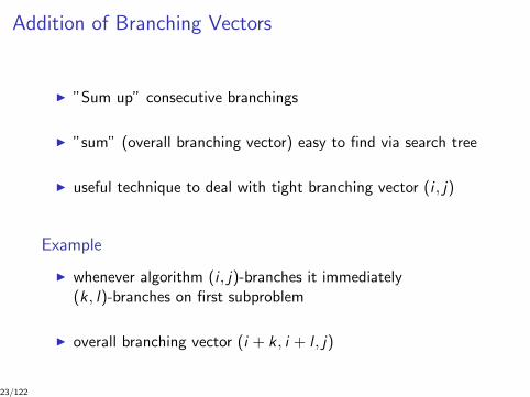
Addition of Branching Vectors

I ”Sum up” consecutive branchings

I ”sum” (overall branching vector) easy to find via search tree

I useful technique to deal with tight branching vector (i , j)

Example

I whenever algorithm (i , j)-branches it immediately(k, l)-branches on first subproblem

I overall branching vector (i + k, i + l , j)

23/122

Addition of Branching Vectors: Example

24/122

III. Preface

25/122

Branching algorithms

I one of the major techniques to construct FPT and ModExAlgorithms

I need only polynomial space

I major progress due to new methods of running time analysis

I many best known ModEx algorithms are branching algorithms

Challenging Open Problem

How to determine worst case running time of branchingalgorithms?

26/122

History: Before the year 2000

I Davis, Putnam (1960): SAT

I Davis, Logemann, Loveland (1962): SAT

I Tarjan, Trojanowski (1977): Independent Set

I Robson (1986): Independent Set

I Monien, Speckenmeyer (1985): 3-SAT

27/122

History: After the Year 2000

I Beigel, Eppstein (2005): 3-Coloring

I Fomin, Grandoni, Kratsch (2005): Dominating Set

I Fomin, Grandoni, Kratsch (2006): Independent Set

I Razgon; Fomin, Gaspers, Pyatkin (2006): FVS

28/122

IV. Our Second Independent Set Algorithm:

mis2

29/122

Branching Rule

I For every vertex v :

I ”either there is a maximum independent set containing v ,

I or there is a maximum independent set containing a neighbourof v”.

I Branching into d(v) + 1 smaller subproblems: ”select v” and”select y” for every y ∈ N(v)

I Branching rule:

α(G ) = max1 + α(G − N[u]) : u ∈ N[v ]

30/122

Algorithm mis2


if (|V | = 0) return 0;

choose a vertex v of minimum degree in G

return 1 + max mis2(G − N[y ]) : y ∈ N[v ];

31/122

Analysis of the Running Time

I Input Size number n of vertices of input graph

I Recurrence:

T (n) ≤ (d + 1) · T (n − d − 1),

where d is the degree of the chosen vertex v .

I Solution of recurrence:

O∗((d + 1)n/(d+1))

(maximum d = 2)

I Running time of mis2: O∗(3n/3).

32/122

Enumerating all maximal independent sets I

Theorem :Algorithm mis2 enumerates all maximal independent sets of theinput graph G in time O∗(3n/3).

I to any leaf of the search tree a maximal independent set of Gis assigned

I each maximal independent set corresponds to a leaf of thesearch tree

Corollary :

A graph on n vertices has O∗(3n/3) maximal independent sets.

33/122

Enumerating all maximal independent sets II

Moon Moser 1962The largest number of maximal independent sets in a graph on nvertices is 3n/3.

Papadimitriou Yannakakis 1984

There is a listing algorithm for the maximal independent sets of agraph having polynomial delay.

34/122

V. Our Third Independent Set Algorithm:

mis3

35/122

Contents

I History of branching algorithms to compute a maximumindependent set

I Branching and reduction rules for Independent Set algorithms

I Algorithm mis3

I Running time analysis of algorithm mis3

36/122

History

Branching Algorithms for Maximum Independent Set

I O(1.2600n) Tarjan, Trojanowski (1977)

I O(1.2346n) Jian (1986)

I O(1.2278n) Robson (1986)

I O(1.2202n) Fomin, Grandoni, Kratsch (2006)

37/122

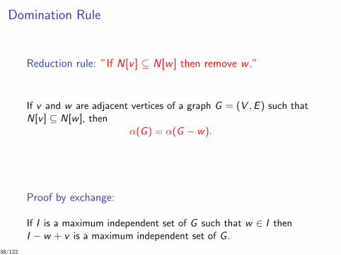
Domination Rule

Reduction rule: ”If N[v ] ⊆ N[w ] then remove w .”

If v and w are adjacent vertices of a graph G = (V ,E ) such thatN[v ] ⊆ N[w ], then

α(G ) = α(G − w).

Proof by exchange:

If I is a maximum independent set of G such that w ∈ I thenI − w + v is a maximum independent set of G .

38/122

Standard branching: ”select v” and ”discard v”

α(G ) = max(1 + α(G − N[v ]), α(G − v)).

To be refined soon.

39/122

”Discard v” implies ”Select two neighbours of v”

Lemma:

Let v be a vertex of the graph G = (V ,E ). If no maximumindependent set of G contains v then every maximum independentset of G contains at least two vertices of N(v).

Proof by exchange: Assume no maximum independent setcontaining v .

I If I is a mis containing no vertex of N[v ] then I + v is a mis,contraction.

I If I is a mis such that v /∈ I and I ∩ N(v) = w, thenI − w + v is a mis of G , contradiction.

40/122

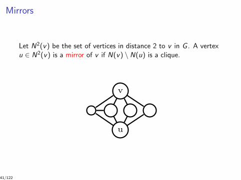
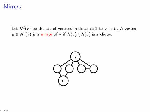
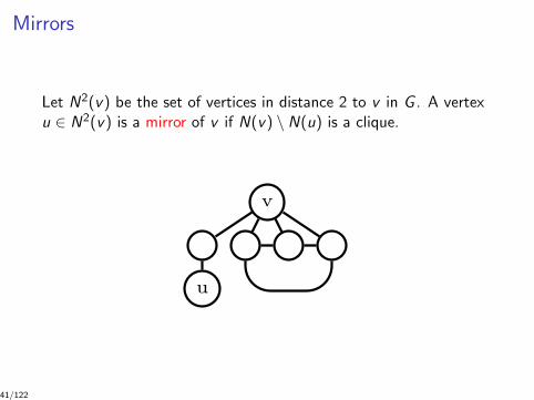
Mirrors

Let N2(v) be the set of vertices in distance 2 to v in G . A vertexu ∈ N2(v) is a mirror of v if N(v) \ N(u) is a clique.

Lemma 3 (folding) Consider a graph G, and let !G(v) be the graph obtained by folding afoldable vertex v. Then

!(G) = 1 + !( !G(v)).

Proof. Let S be a maximum independent set of G. If v ! S, then S \v is an independentset of !G(v). Otherwise, S contains at least one vertex of N(v) (since it is of maximumcardinality). If N(v)"S = u, then S\u is an independent set of !G(v). Otherwise, it mustbe N(v) " S = ui, uj, for two non-adjacent vertices ui and uj (since N(v) does not containany anti-triangle by assumption). In this case S#uij\ui, uj is an independent set of !G(v).It follows that !(G) $ 1 + !( !G(v)). A similar argument shows that !(G) % 1 + !( !G(v)). !

We eventually introduce the following useful notion of mirror. Given a vertex v, a mirrorof v is a vertex u ! N 2(v) such that N(v) \N(u) is a (possibly empty) clique. We denote byM(v) the set of mirrors of v. Examples of mirrors are given in Figure 4. Intuitively, when

Figure 4 Example of mirrors: u is a mirror of v.

v

u

v

u

v

u

v

u

we discard a vertex v, we can discard its mirrors as well without modifying the maximumindependent set size. This intuition is formalized in the following lemma.

Lemma 4 (mirroring) For any graph G and for any vertex v of G,

!(G) = max!(G & v & M(v)), 1 + !(G & N [v]).

Proof. Vertex v can either belong to a maximum independent set or not, from which weobtain the trivial equation

!(G) = max!(G & v), 1 + !(G & N [v]).

Thus it is su!cient to show that, if v is not contained in any maximum independent set,the same holds for its mirrors M(v). Following the proof of Lemma 2, if no maximumindependent set contains v, every maximum independent set contains at least two verticesin N(v). Consider a mirror u ! M(v). Since every independent set contains at most onevertex in N(v) \ N(u) (which is a clique by assumption), it must contain at least one vertexin N(v)"N(u) ' N(u). It follows that u is not contained in any maximum independent set.

!

4.2 The Algorithm

Our algorithm mis is described in Figure 5. In the base case |V (G)| $ 1, the algorithmreturns the optimum solution mis(G) = |V (G)| (line 1). Otherwise, mis tries to reduce thesize of the problem by applying Lemma 2 and Lemma 3. Specifically, if G contains a properconnected component C (line 2), the algorithm recursively solves the subproblems inducedby C and G & C separately, and sums the solutions obtained

mis(G) = mis(C) + mis(G & C).

17

41/122

Mirror Branching

Mirror Branching: Refined Standard Branching

If v is a vertex of the graph G = (V ,E ) and M(v) the set ofmirrors of v then

α(G ) = max(1 + α(G − N[v ]), α(G − (M(v) + v)).

Proof by exchange: Assume no mis of G contains v

I By the lemma, every mis of G contains two vertices of N(v).

I If u is a mirror then N(v) \ N(u) is a clique; thus at least onevertex of every mis belongs to N(u).

I Consequently, no mis contains u.

42/122

Simplicial Rule

Reduction Rule: Simplicial Rule

Let G = (V ,E ) be a graph and v be a vertex of G such that N[v ]is a clique. Then

α(G ) = 1 + α(G − N[v ]).

Proof:Every mis contains v by the Lemma.

43/122

Branching on Components

Component Branching

Let G = (V ,E ) be a disconnected graph and let C be acomponent of G . Then

α(G ) = α(G − C ) + α(C ).

Well-known property of the independence number α(G ).

44/122

Separator branching

S ⊆ V is a separator of G = (V ,E ) if G − S is disconnected.

Separator Branching: ”Branch on all independent sets ofseparator S”.

If S is a separator of the graph G = (V ,E ) and I(S) the set of allindependent subsets I ⊆ S of G , then

α(G ) = maxA∈I(S)

|A| + α(G − (S ∪ N[A])).

45/122

46/122

Using Separator Branching

I separator S small, and

I easy to find.

mis3 uses ”separator branching on S” only if

I S ⊆ N2(v), and

I |S | ≤ 2

47/122

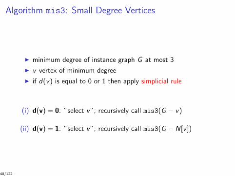
Algorithm mis3: Small Degree Vertices

I minimum degree of instance graph G at most 3

I v vertex of minimum degree

I if d(v) is equal to 0 or 1 then apply simplicial rule

(i) d(v) = 0: ”select v”; recursively call mis3(G − v)

(ii) d(v) = 1: ”select v”; recursively call mis3(G − N[v ])

48/122

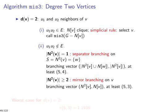
Algorithm mis3: Degree Two Vertices

I d(v) = 2: u1 and u2 neighbors of v

(i) u1u2 ∈ E : N[v ] clique; simplicial rule: select v .call mis3(G − N[v ])

(ii) u1u2 /∈ E .

|N2(v)| = 1 : separator branching onS = N2(v) = wbranching vector (|N2[v ] ∪ N[w ]|, |N2[v ]|), atleast (5, 4).

|N2(v)| ≥ 2 : mirror branching on v

branching vector (N2[v ],N[v ]), at least (5, 3).

Worst case for d(v) = 2:

τ(5, 3) = 1.193949/122

50/122

Analysis for d(v) = 2

|N2(v)| = 1 : separator branching on S = N2(v) = w

Subproblem 1: ”select v and w” call mis3(G − (N[v ] ∪ N[w ]))Subproblem 2: ”select u1 and u2”; call mis3(G − N2[v ])

Branching vector (|N[v ] ∪ N[w ]|, |N2[v ]|) ≥ (5, 4).

|N2(v)| ≥ 2 : mirror branching on v

”discard v”: select both neighbors of v , u1 and u2

”select” v”: call mis3(G − N[v ])

Branching vector (|N2[v ]|, |N[v ]|) ≥ (5, 3)

51/122

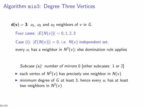
Algorithm mis3: Degree Three Vertices

d(v) = 3: u1, u2 and u3 neighbors of v in G .

Four cases: |E (N(v))| = 0, 1, 2, 3

Case (i): |E (N(v))| = 0, i.e. N(v) independent set.

every ui has a neighbor in N2(v); else domination rule applies

Subcase (a): number of mirrors 0 [other subcases: 1 or 2]

I each vertex of N2(v) has precisely one neighbor in N(v)

I minimum degree of G at least 3, hence every ui has at leasttwo neighbors in N2(v)

52/122

53/122

d(v) = 3, N(v) independent set, v has no mirror

Algorithm branches into four subproblems:

I select v

I discard v , select u1, select u2

I discard v , select u1, discard u2, select u3

I discard v , discard u1, select u2, select u3

Branching vector (4, 7, 8, 8) and τ(4, 7, 8, 8) = 1.2406.

More subcases. More Cases. ...

Exercice:Analyse the Subcases (b) and (c) of Case (i), and Case (ii).

54/122

Algorithm mis3: Degree Three Vertices

Case (iii): |E (N(x))| = 2.u1u2 and u2u3 edges of N(v).

Mirror branching on v :

”select v”: call mis3(G − N[v ])”discard v”: discard v , select u1 and u3

Branching factor (4, 5) and τ(4, 5) = 1.1674

Case (iv): |E (N(x))| = 3.simplicial rule: ”select v”


τ(4, 7, 8, 8) = 1.2406

55/122

Algorithm mis3: Large Degree Vertices

Maximum Degree Rule [δ(G ) ≥ 4]

”Mirror Branching on a maximum degree vertex”

d(v) ≥ 6:

mirror branching on v

Branching vector (d(v) + 1, 1) ≥ (7, 1)

Worst case for d(v) ≥ 6:

τ(7, 1) = 1.2554

56/122

Algorithm mis3: Regular Graphs

Mirror branching on r -regular graph instances:

Not taken into account !

For every r , on any path of the search tree from the root to a leafthere is only one r -regular graph.

57/122

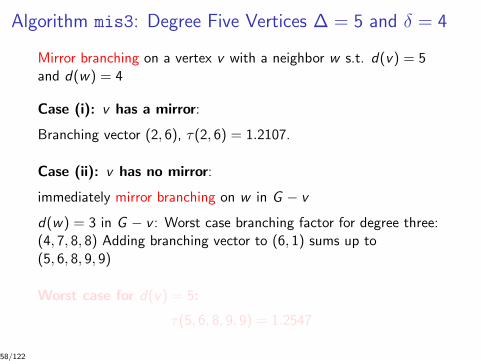
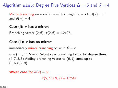
Algorithm mis3: Degree Five Vertices ∆ = 5 and δ = 4

Mirror branching on a vertex v with a neighbor w s.t. d(v) = 5and d(w) = 4

Case (i): v has a mirror:

Branching vector (2, 6), τ(2, 6) = 1.2107.

Case (ii): v has no mirror:

immediately mirror branching on w in G − v

d(w) = 3 in G − v : Worst case branching factor for degree three:(4, 7, 8, 8) Adding branching vector to (6, 1) sums up to(5, 6, 8, 9, 9)


τ(5, 6, 8, 9, 9) = 1.2547

58/122

59/122

Running time of Algorithm mis 3

Theorem :Algorithm mis3 runs in time O∗(1.2554n).

Theorem :The algorithm of Tarjan and Trojanowski has running timeO∗(2n/3) = O∗(1.2600n). [O∗(1.2561n)]

60/122

VI. A DPLL Algorithm

61/122

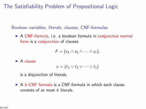
The Satisfiability Problem of Propositional Logic

Boolean variables, literals, clauses, CNF-formulas

I A CNF-formula, i.e. a boolean formula in conjunctive normalform is a conjunction of clauses

F = (c1 ∧ c2 ∧ · · · ∧ cr ).

I A clausec = (`1 ∨ `2 ∨ · · · ∨ `t)

is a disjunction of literals.

I A k-CNF formula is a CNF-formula in which each clauseconsists of at most k literals.

62/122

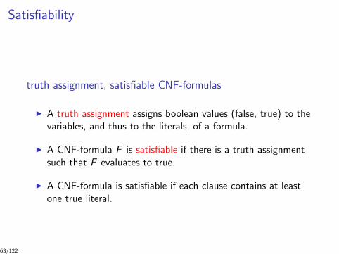
Satisfiability

truth assignment, satisfiable CNF-formulas

I A truth assignment assigns boolean values (false, true) to thevariables, and thus to the literals, of a formula.

I A CNF-formula F is satisfiable if there is a truth assignmentsuch that F evaluates to true.

I A CNF-formula is satisfiable if each clause contains at leastone true literal.

63/122

The Problems SAT and k-SAT

Definition (Satisfiability (SAT))

Given a CNF-formula F , decide whether F is satisfiable.

Definition (k-Satisfiability (k-SAT))

Given a k-CNF F , decide whether F is satisfiable.

F = (x1 ∨ ¬x3 ∨ x4) ∧ (¬x1 ∨ x3 ∨ ¬x4) ∧ (¬x2 ∨ ¬x3 ∨ x4)

64/122

Reduction and Branching Rules of a Classical DPLLalgorithm

I Davis, Putnam 1960

I Davis, Logemann, Loveland (1962)

Reduction and Branching Rules

I [UnitPropagate] If all literals of a clause c except literal ` arefalse (under some partial assignment), then ` must be set totrue.

I [PureLiteral] If a literal ` occurs pure in F , i.e. ` occurs in Fbut its negation does not occur, then ` must be set to true.

I [Branching] For any variable xi , branch into ”xi true” and ”xi

false”.

65/122

VII. The algorithm of Monien and

Speckenmeyer

66/122

Assigning Truth Values via Branching

I Recursively compute partial assignment(s) of given k-CNFformula F

I Given a partial truth assignment of F the correspondingk-CNF formula F ′ is obtained by removing all clausescontaining a true literal, and by removing all false literals.

I Subproblem generated by the branching algorithm is a k-CNFformula

I Size of a k-CNF formula is its number of variables

67/122

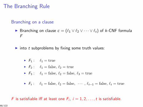
The Branching Rule

Branching on a clause

I Branching on clause c = (`1 ∨ `2 ∨ · · · ∨ `t) of k-CNF formulaF

I into t subproblems by fixing some truth values:

I F1 : `1 = trueI F2 : `1 = false, `2 = trueI F3 : `1 = false, `2 = false, `3 = true

I Ft : `1 = false, `2 = false, · · · , `t−1 = false, `t = true

F is satisfiable iff at least one Fi , i = 1, 2, . . . , t is satisfiable.

68/122

Time Analysis I

I Assuming F consists of n variables then Fi , i = 1, 2, . . . , t,consists of n − i (non fixed) variables.

I Branching vector is (1, 2, . . . , t), where t = |c |.

I Solve linear recurrenceT (n) ≤ T (n − 1) + T (n − 2) + · · ·+ T (n − t).

I Compute the unique positive real root of

x t = x t−1 + x t−2 + x t−3 + · · ·+ 1 = 0

which is equivalent to

x t+1 − 2x t + 1 = 0.

69/122

Time Analysis II

For a clause of size t, let βt be the branching factor.

Branching Factors: β2 = 1.6181, β3 = 1.8393, β4 = 1.9276,β5 = 1.9660, etc.

There is a branching algorithm solving 3-SAT in time O∗(1.8393n).

70/122

Speeding Up the Branching Algorithm

Observation: ”The smaller the clause the better the branchingfactor.”

Key Idea: Branch on a clause c of minimum size. Make sure that|c | ≤ k − 1.

Halting and Reduction Rules:

I If |c | = 0 return ”unsatisfiable”.

I If |c | = 1 reduce by setting the unique literal true.

I If F is empty then return ”satisfiable”.

71/122

Monien Speckenmeyer 1985

For any k ≥ 3, there is an O∗(βk−1n) algorithm to solve k-SAT.

3-SAT can be solved by an O∗(1.6181n) time branching algorithm.

72/122

Autarky: Key Properties

DefinitionA partial truth assignment t of a CNF formula F is called autark iffor every clause c of F for which the value of at least one literal isset by t, there is a literal `i of c such that t(`i ) = true.

Let t be a partial assignment of F .

I t autark: Any clause c for which a literal is set by t is true.Thus F is satisfiable iff F ′ is satisfiable, where F ′ is obtainedby removing all clauses c set true by t.

⇒ reduction rule

I t not autark: There is a clause c for which a literal is set byt but c is not true under t. Thus in the CNF-formulacorresponding to t clause c has at most k − 1 literals.

⇒ branch always on a clause of at most k − 1 literals73/122

VIII. Lower Bounds

74/122

Time Analysis of Branching Algorithms

Available Methods

I simple (or classical) time analysis

I Measure & Conquer, quasiconvex analysis, etc.

I based on recurrences

What can be achieved?

I establish upper bounds on the (worst-case) running time

I new methods achieve improved bounds for same algorithm

I no proof for tightness of bounds

75/122

Limits of Current Time Analysis

We cannot determine the worst-case running time of branchingalgorithms !

Consequences

I stated upper bounds of algorithms may (significantly)overestimate running times

I How to compare branching algorithms if their worst-caserunning time is unknown?

We strongly need better methods for Time Analysis !

Better Methods of Analysis lead to Better Algorithms

76/122

Why study Lower Bounds of Worst-Case Running Time?

I Upper bounds on worst case running time of a Branchingalgorithms seem to overestimate the running time.

I Lower bounds on worst case running time of a particularbranching algorithm can give an idea how far current analysisof this algorithm is from being tight.

I Large gaps between lower and upper bounds for someimportant branching algorithms.

I Study of lower bounds leads to new insights on particularbranching algorithm.

77/122

Algorithm mis1 Revisited






78/122

Algorithm mis1a


if (∆(G ) ≥ 3) choose a vertex v of maximum degree




79/122

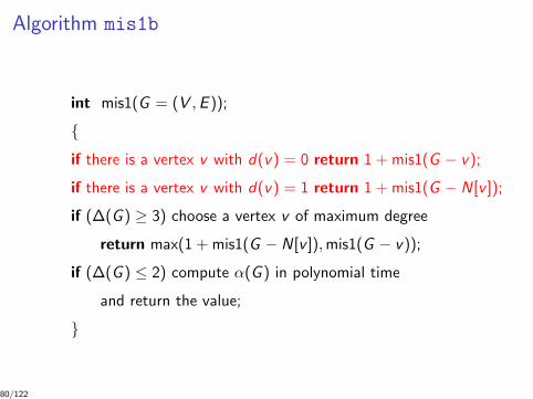
Algorithm mis1b


if there is a vertex v with d(v) = 0 return 1 + mis1(G − v);

if there is a vertex v with d(v) = 1 return 1 + mis1(G − N[v ]);

if (∆(G ) ≥ 3) choose a vertex v of maximum degree




80/122

Upper Bounds of Running time

Simple Running Time Analysis

I Branching vectors of standard branching: (1, d(v) + 1)

I Running time of algorithm mis1: O∗(1.3803n)

I Running time of modifications mis1a and mis1b:O∗(1.3803n)

Does all three algorithms have same worst-caserunning time ?

81/122

Related Questions

I What is the worst-case running time of these three algorithmson graphs of maximum degree three?

I How much can we improve the upper bounds of the runningtimes of those three algorithms by Measure & Conquer?

I (Again) what is the worst-case running time of algorithmmis1?

82/122

A lower bound for mis1

Lower bound graph

I Consider the graphs Gn = (Vn,E3)

I Vertex set: 1, 2, . . . , nI Edge set: i , j ∈ E3 ⇔ |i − j | ≤ 3

83/122

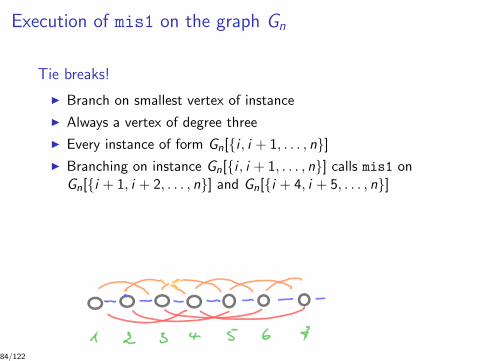
Execution of mis1 on the graph Gn

Tie breaks!

I Branch on smallest vertex of instance

I Always a vertex of degree three

I Every instance of form Gn[i , i + 1, . . . , n]I Branching on instance Gn[i , i + 1, . . . , n] calls mis1 on

Gn[i + 1, i + 2, . . . , n] and Gn[i + 4, i + 5, . . . , n]

84/122

Recurrence for lower bound of worst-case running time:

T (n) = T (n − 1) + T (n − 4)

Theorem:The worst-case running time of algorithm mis1 is Θ∗(cn), wherec = 1.3802... is the unique positive root of x4 − x3 − 1.

Exercice:Determine lower bounds for the worst-case running time of mis1aand mis1b.

85/122

Algorithm mis2 Revisited


if (|V | = 0) return 0;

choose a vertex v of minimum degree in G

return 1 + max mis2(G − N[y ]) : y ∈ N[v ];

Theorem:The running time of algorithm mis2 is O∗(3n/3). Algorithm mis2enumerates all maximal independent sets of the input graph.

86/122

A lower bound for mis2

a1 b1

c1

a2 b2

c2

ak bk

ck

I Lower bound graph Gk : disjoint union of k triangles.

I Algorithm mis2 applied to Gk : chooses a vertex of anytriangle, branches into three subproblems Gk−1;(by removing a triangle from Gk)

I Search tree has 3k = 3n/3 leaves;

Theorem:The worst-case running time of algorithm mis2 is Θ∗(3n/3).

87/122

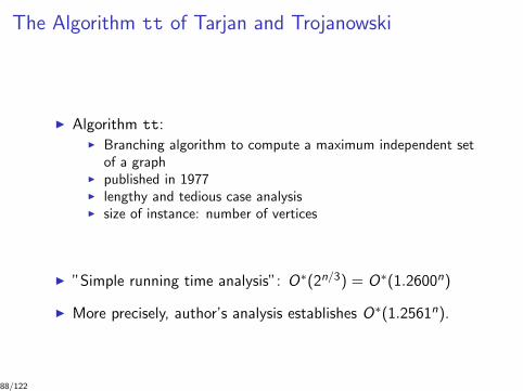
The Algorithm tt of Tarjan and Trojanowski

I Algorithm tt:I Branching algorithm to compute a maximum independent set

of a graphI published in 1977I lengthy and tedious case analysisI size of instance: number of vertices

I ”Simple running time analysis”: O∗(2n/3) = O∗(1.2600n)

I More precisely, author’s analysis establishes O∗(1.2561n).

88/122

Important Properties of tt

Minimum Degree at most 4

If the minimum degree of the problem instance G is at most 4 thenalgorithm tt runs through plenty of cases.

Minimum Degree at least 5

Either G is 5-regular or algorithm tt“chooses ANY vertex w of degree at least 6 and branches toG − N[w ] (select w) and G − w (discard w)”.

Lower bound graphs of minimum degree 6

89/122

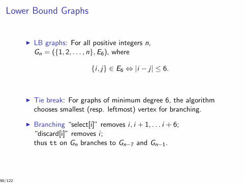
Lower Bound Graphs

I LB graphs: For all positive integers n,Gn = (1, 2, . . . , n,E6), where

i , j ∈ E6 ⇔ |i − j | ≤ 6.

I Tie break: For graphs of minimum degree 6, the algorithmchooses smallest (resp. leftmost) vertex for branching.

I Branching “select[i]” removes i , i + 1, . . . i + 6;“discard[i]” removes i ;thus tt on Gn branches to Gn−7 and Gn−1.

90/122

Branching

1 2 3 4 5 6 7 8 9 n

discard 1 select 1

2 3 4 5 6 7 8 9 n 8 9 n

91/122

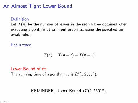
An Almost Tight Lower Bound

DefinitionLet T (n) be the number of leaves in the search tree obtained whenexecuting algorithm tt on input graph Gn using the specified tiebreak rules.

Recurrence

T (n) = T (n − 7) + T (n − 1)

Lower Bound of ttThe running time of algorithm tt is Ω∗(1.2555n).

REMINDER: Upper Bound O∗(1.2561n).

92/122

Do we need lower bounds for other ModEx algorithms?

I Dynamic Programming

I Inclusion-Exclusion

I Treewidth Based

I Subset Convolution

93/122

Often claimed: ”Our algorithm is faster on practical instances thanits (worst case running) time we claim.”

For branching algorithms the situation seems to be even better:

I faster than claimed running time on all instances

I hard to construct instances that even need a close runningtime

I ”much better on many instances”?

94/122

IX. Memorization

95/122

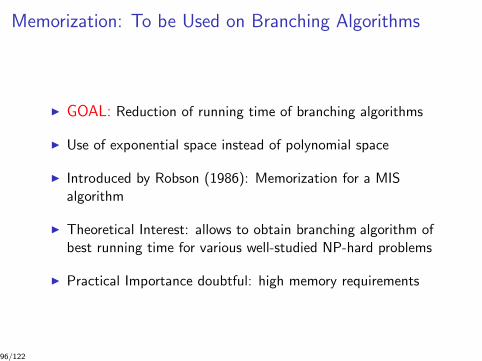
Memorization: To be Used on Branching Algorithms

I GOAL: Reduction of running time of branching algorithms

I Use of exponential space instead of polynomial space

I Introduced by Robson (1986): Memorization for a MISalgorithm

I Theoretical Interest: allows to obtain branching algorithm ofbest running time for various well-studied NP-hard problems

I Practical Importance doubtful: high memory requirements

96/122

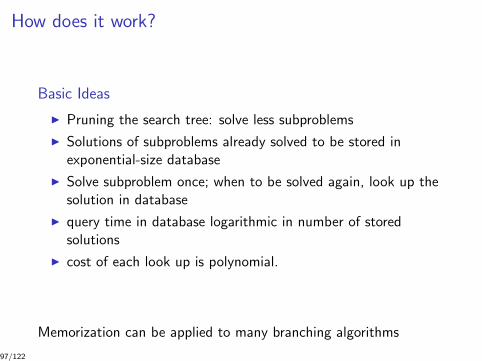
How does it work?

Basic Ideas

I Pruning the search tree: solve less subproblems

I Solutions of subproblems already solved to be stored inexponential-size database

I Solve subproblem once; when to be solved again, look up thesolution in database

I query time in database logarithmic in number of storedsolutions

I cost of each look up is polynomial.

Memorization can be applied to many branching algorithms

97/122

Once again Algorithm mis1






Theorem:Algorithm mis1 has running time O∗(1.3803n) and uses onlypolynomial space.

98/122

Reduction of the Running Time of mis1

The algorithm

I Having solved an instance G ′, an induced subgraph of inputgraph G , store (G ′, α(G ′)) in a database.

I Before solving any instance, check whether its solution isalready available in database.

I Input graph G has at most 2n induced subgraphs.

I Database can be implemented such that each query takestime logarithmic in its size, thus polynomial in n.

99/122

Analysis of the Exponential Space algorithm

Upper bound of the running time of original polynomial spacebranching algorithm is needed to analyse the exponential spacealgorithm.

I Search tree of mis1(G ) on any graph of n vertices has T (n)leaves: T (n) ≤ 1.3803n.

I Let Th(n), 0 ≤ h ≤ n, be the maximum number ofsubproblems of size h solved when calling mis1(G ) for anygraph of n.

I Th(n) maximum number of nodes of the subtreecorresponding to an instance of h vertices.

I Similar to analysis of T (n), one obtains:

Th(n) ≤ 1.3803n−h

100/122

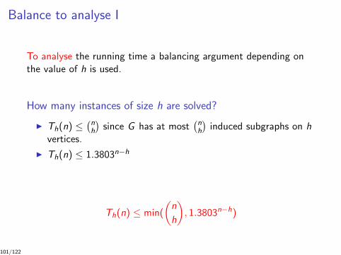
Balance to analyse I

To analyse the running time a balancing argument depending onthe value of h is used.

How many instances of size h are solved?

I Th(n) ≤(nh

)since G has at most

(nh

)induced subgraphs on h

vertices.

I Th(n) ≤ 1.3803n−h

Th(n) ≤ min(

(n

h

), 1.3803n−h)

101/122

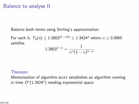
Balance to analyse II

Balance both terms using Stirling’s approximation:

For each h, Th(n) ≤ 1.3803(1−α)n ≤ 1.3424n where α ≥ 0.0865satisfies

1.38031−α =1

αα(1− α)1−α

Theorem:Memorization of algorithm mis1 establishes an algorithm runningin time O∗(1.3424n) needing exponential space.

102/122

X. Branch & Recharge

103/122

Another Way to Design and Analyse Branching Algorithms

I Using weights within the algorithm; not ”only” as a tool inanalysis

I GOAL: Easy time analysis

I In the best case: a few simple recurrences to solve

I Sophisticated correctness proof

I Time analysis (still) ”recurrence based”

104/122

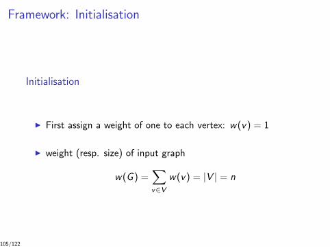
Framework: Initialisation

Initialisation

I First assign a weight of one to each vertex: w(v) = 1

I weight (resp. size) of input graph

w(G ) =∑v∈V

w(v) = |V | = n

105/122

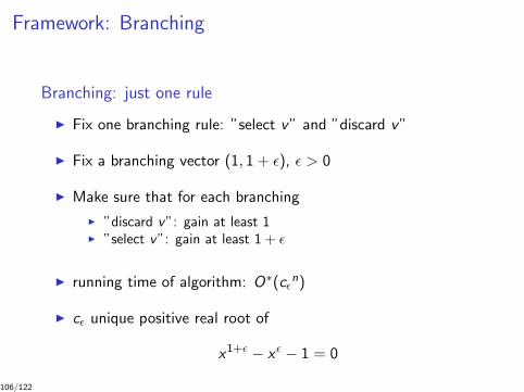
Framework: Branching

Branching: just one rule

I Fix one branching rule: ”select v” and ”discard v”

I Fix a branching vector (1, 1 + ε), ε > 0

I Make sure that for each branching

I ”discard v”: gain at least 1I ”select v”: gain at least 1 + ε

I running time of algorithm: O∗(cεn)

I cε unique positive real root of

x1+ε − xε − 1 = 0

I cε < 2

106/122

Framework: Recharging

Recharging

I When branching on a vertex v with w(v) = 1,

set w(v) = 0 in both subproblems

I ”select v”: Borrow a weight of ε from a neighbour of v

I When branching on a vertex v with w(v) < 1Recharge the weight of v to 1, before branching on v

107/122

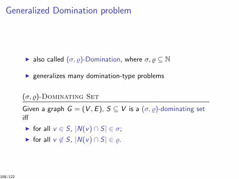
Generalized Domination problem

I also called (σ, %)-Domination, where σ, % ⊆ N

I generalizes many domination-type problems

(σ, %)-Dominating Set

Given a graph G = (V ,E ), S ⊆ V is a (σ, %)-dominating setiff

I for all v ∈ S , |N(v) ∩ S | ∈ σ;

I for all v 6∈ S , |N(v) ∩ S | ∈ %.

108/122

An Example

i

j

a b

c

d

e f

g

h

Let σ = 0, 1 and % = 2, 4, 8.

Gray vertices form a (σ, %)-Dominating Set.

109/122

σ and % finite

Choice of ε

εp,q =1

max(p, q),

where p = maxσ and q = max ρ.

Example: Perfect Code

σ = 0, and ρ = 1.

ε = 1.

110/122

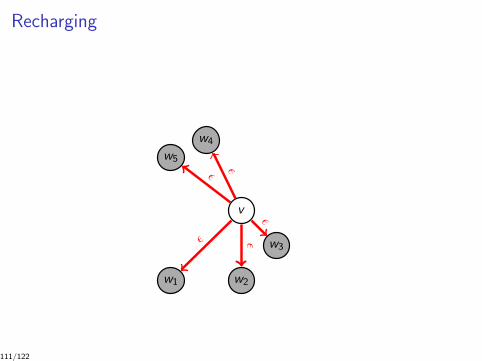
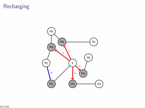
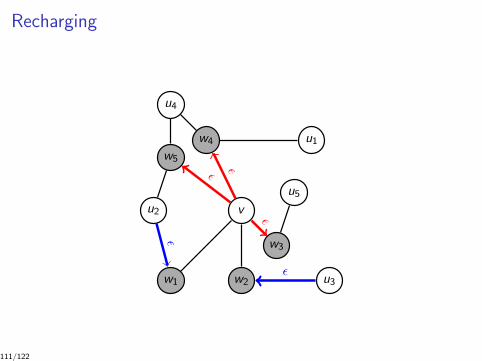
Recharging

! domination classes de graphes clique dominante (!, ")-domination "

Le rechargement

v

w1 w2

w3

w4

w5

! !!

!

!

Les sommets en gris sont dans l’ensemble (", #)-dominant ;on n’a pas encore branche sur les autres sommets.

w(v) = 1

60/64

111/122

Recharging


Le rechargement

v

w1 w2

w3

w4

w5

u1

u2

u3

u4

u5

! !!

!

!


w(v) = 1

60/64

111/122

Recharging


Le rechargement

v

w1 w2

w3

w4

w5

u1

u2

u3

u4

u5

!!

!

!

!Les sommets en gris sont dans l’ensemble (", #)-dominant ;

on n’a pas encore branche sur les autres sommets.

w(v) = 1

60/64

111/122

Recharging


Le rechargement

v

w1 w2

w3

w4

w5

u1

u2

u3

u4

u5

!

!

!

!

!


w(v) = 1

60/64

111/122

Recharging


Le rechargement

v

w1 w2

w3

w4

w5

u1

u2

u3

u4

u5

!

!

!

!!


w(v) = 1

60/64

111/122

Recharging


Le rechargement

v

w1 w2

w3

w4

w5

u1

u2

u3

u4

u5

!

!

!!

!


w(v) = 1

60/64

111/122

Recharging


Le rechargement

v

w1 w2

w3

w4

w5

u1

u2

u3

u4

u5

!

!!

!

!


w(v) = 1

60/64

111/122

We hope that Branch & Recharge will prove its potential asanother method to design and analyse branching algorithms.

112/122

XI. Exercices

113/122

Exercices I

1. The HAMILTONIAN CIRCUIT problem can be solved in timeO∗(2n) via dynamic programming or inclusion-exclusion. Constructa O∗(3m/3) branching algorithm deciding whether a graph has ahamiltonian circuit, where m is the number of edges.

2. Let G = (V ,E ) be a bicolored graph, i.e. its vertices are eitherred or blue. Construct and analyze branching algorithms that forinput G , k1, k2 decide whether the bicolored graph G has anindependent set I with k1 red and k2 blue vertices. What is thebest running time you can establish?

3. Construct a branching algorithm for the 3-COLORING problem,i.e. for given graph G it decides whether G is 3-colorable. Therunning time should be O∗(3n/3) or even O∗(cn) for some c < 1.4.

114/122

Exercices II

4. Construct a branching algorithm for the DOMINATING SETproblem on graphs of maximum degree 3.

5. Is the following statement true for all graphs G : ”If w is amirror of v and there is a maximum independent set of G notcontaining v , then there is a maximum independent set containingneither v nor w .”

6. Modify the first IS algorithm such that it always branches on amaximum degree vertex. Provide a lower bound (for mis1a).What is the worst-case running time of this algorithm?

115/122

Exercices III

7. Modify the first IS algorithm such that it uses a reduction ruleson vertex of minimum degree, if it is 0 or 1, and if no such vertexexists it branches on a maximum degree vertex (of degree greaterthan three). Provide a lower bound (for mis1b). What is theworst-case running time of this algorithm?

8. Construct a O∗(1.49n) branching algorithm to solve 3-SAT.

116/122

More Exercices

Construct and analyse branching algorithms for the followingproblems:

I Perfect Cover: Given a graph, decide whether it has a vertexset I such that every vertex v of G belongs to precisely oneneighbourhood set N[u] for any u ∈ I .

I Max 2-SAT: Given a 2-CNF formula F , compute a truthassignment of its variables which maximizes the number oftrue clauses of F .

I Weighted Independent Set: Given a graph G = (V ,E )with positive integral vertex weights, compute a maximumweight independent set of G .

117/122

XII. For Further Reading

118/122

T.H. Cormen, C.E. Leiserson, R.L. Rivest, C. Stein,Introduction to Algorithms,MIT Press, 2001.

J. Kleinberg, E. Tardos,Algorithm Design,Addison-Wesley, 2005.

R.L. Graham, D.E. Knuth, O. PatashnikConcrete Mathematics,Addison-Wesley, 1989.

R. Beigel and D. Eppstein.3-coloring in time O(1.3289n).Journal of Algorithms 54:168–204, 2005.

M. Davis, G. Logemann, and D.W. Loveland,A machine program for theorem-proving.Communications of the ACM 5:394–397, 1962.

119/122

M. Davis, H. Putnam.A computing procedure for quantification theory.Journal of the ACM 7:201–215, 1960.

D. Eppstein.The traveling salesman problem for cubic graphs.Proceedings of WADS 2003, pp. 307–318.

F. V. Fomin, S. Gaspers, and A. V. Pyatkin.Finding a minimum feedback vertex set in time O(1.7548n),Proceedings of IWPEC 2006, Springer, 2006, LNCS 4169,pp. 184–191.

F. V. Fomin, P. Golovach, D. Kratsch, J. Kratochvil and M.Liedloff.Branch and Recharge: Exact algorithms for generalizeddomination.Proceedings of WADS 2007, Springer, 2007, LNCS 4619, pp.508–519.

120/122

F. V. Fomin, F. Grandoni, D. Kratsch.Some new techniques in design and analysis of exact(exponential) algorithms.Bulletin of the EATCS 87:47–77, 2005.

F. V. Fomin, F. Grandoni, D. Kratsch.Measure and Conquer: A Simple O(20.288 n) Independent SetAlgorithm.Proceedings of SODA 2006, ACM and SIAM, 2006, pp.508–519.

K. Iwama.Worst-case upper bounds for k-SAT.Bulletin of the EATCS 82:61–71, 2004.

K. Iwama and S. Tamaki.Improved upper bounds for 3-SAT.Proceedings of SODA 2004, ACM and SIAM, 2004, p. 328.

121/122

O. Kullmann.New methods for 3-SAT decision and worst case analysis.Theoretical Computer Science 223: 1–72, 1999.

B. Monien, E. Speckenmeyer.Solving satisfiability in less than 2n steps.Discrete Appl. Math. 10: 287–295, 1985.

I. Razgon.Exact computation of maximum induced forest.Proceedings of SWAT 2006, Springer, 2006, LNCS 4059,pp. 160–171.

J. M. Robson.Algorithms for maximum independent sets.Journal of Algorithms 7(3):425–440, 1986.

R. Tarjan and A. Trojanowski.Finding a maximum independent set.SIAM Journal on Computing, 6(3):537–546, 1977.

122/122

G. J. Woeginger.Exact algorithms for NP-hard problems: A survey.Combinatorial Optimization – Eureka, You Shrink, Springer,2003, LNCS 2570, pp. 185–207.

G. J. Woeginger.Space and time complexity of exact algorithms: Some openproblems.Proceedings of IWPEC 2004, Springer, 2004, LNCS 3162,pp. 281–290.

G. J. Woeginger.Open problems around exact algorithms.Discrete Applied Mathematics, 156:397–405, 2008.

123/122

branching algorithms - inria · branching algorithms are also called i branch & bound...

Documents