interpreting effect sizes in contrast...

TEACHING ARTICLES

Interpreting Effect Sizesin Contrast Analysis

R. Michael FurrDepartment of Psychology

Appalachian State University

Although researchers are becoming more aware of the benefits of reporting effectsizes, the usefulness of effect sizes can be enhanced if researchers have a firm under-standing of how to interpret the various effect sizes that are available. This article ar-ticulates and illustrates the interpretation of 3 pairs of effect sizes developed for use incontrast analysis (Rosenthal, Rosnow, & Rubin, 2000). Three ways of conceptualiz-ing the effect sizes are discussed: (a) as correlations between predicted and observeddata, (b) as proportion of variance accounted for, and (c) as parallel to a multiple re-gression approach. It is hoped that this interpretive aid helps increase the frequencywith which effect sizes are reported and the effectiveness with which they are used.

contrast analysis, effect size, significance testing, correlation

Social scientists are increasingly promoting the importance and utility of effectsizes (e.g., Cohen, 1994). One outcome of the vociferous debate over the role of sig-nificance testing has been a deeper appreciation of the role of effect sizes. In fact,the Publication Manual of the American Psychological Association (AmericanPsychological Association [APA], 2001) tells authors that “For readers to fully un-derstand your findings, it is almost always necessary to include some index of ef-fect size or strength of relation in your Results section” (p. 25). Along with this en-dorsement by APA, a growing number of journals have instituted explicitrequirements or recommendations encouraging the reporting of effect sizes(Keselman et al., 1998; Kirk, 1996; Vacha-Haase, Nilsson, Reetz, Lance, &Thompson, 2000; Wilkinson & The APA Task Force on Statistical Inference,1999).

UNDERSTANDING STATISTICS, 3(1), 1–25Copyright © 2004, Lawrence Erlbaum Associates, Inc.

Requests for reprints should be sent to R. Michael Furr, Department of Psychology, AppalachianState University, Boone, NC 28607. E-mail: [email protected]

Despite the growing appreciation of effect sizes among methodologists, thewider research community appears to be adopting effect sizes rather slowly(Thompson, 1999b). The strong stances recently taken by journal editors and in thePublication Manual of the American Psychological Association (APA, 2001) willlikely accelerate the reporting of effect sizes, but this is only half the battle. Socialresearch will be advanced not only through the reporting effect sizes, but alsothrough the accurate interpretation of effect sizes. As Vacha-Haase et al. (2000)pointed out, “many researchers do not fully understand the logic of their statisticaltests … and therefore may remain oblivious to the need for effect-size reportingand interpretation” (p. 414, italics added). Effect sizes can be most fully appreci-ated and, more important, most usefully interpreted if researchers have a solidgrasp of their logic and meanings. This article describes and illustrates the inter-pretations of several effect sizes in the context of contrast analysis.

Along with an increased appreciation for effect sizes, many researchers haverecently argued for the utility of contrast analyses (e.g., Furr & Rosenthal, 2003a;Loftus, 1996). Contrast analysis is designed to address focused analytic questions;in other words, to evaluate theories efficiently. For example, if a clinical researcherpredicts that a treatment group will show more rapid symptom decrease than a con-trol group, he or she could conduct a contrast analysis to obtain a significance testand effect size directly reflecting the degree to which the obtained pattern of re-sults matches the predicted pattern of results. The popular traditional alternativewould be to compute an analysis of variance (ANOVA) and hope for a significantmain effect and interaction, which would be probed with a series of conservativepost hoc analyses. Such an approach would likely lead to no single significancetest or effect size directly related to the researcher’s specific theoretical prediction.In their comprehensive discussion of contrast analysis, Rosenthal, Rosnow, andRubin (2000) outlined three basic correlational effect sizes. Each of thesecorrelational effect sizes can be interpreted in two ways.

First, as with any correlation, a correlational effect size reflects the associa-tion between two things. Specifically, it can be interpreted as a correlation be-tween the observed data and a theoretically predicted pattern of data. However,to fully understand the meaning of such an effect size, researchers must under-stand which parts of the observed and predicted data are being correlated. Forexample, does the data refer to the individual scores, group means, or an ad-justed set of scores? Second, as with any correlation, a correlational effect sizefrom contrast analysis can be squared and interpreted as “the proportion of vari-ation accounted for” by the contrast. However, to fully understand the meaningof such an effect size, researchers must understand which part of the variation isbeing considered. Is it the total variation, the between-groups variation, or theerror variation?

This article illustrates and articulates the meaning of three fundamental effectsizes associated with contrast analysis. In doing so, it discusses each from both the

2 FURR

“unsquared” and “squared” perspectives: reffect size (and reffectsize2 ), ralerting (and

ralerting2 ), and rcontrast (and rcontrast

2 ). In addition, this article discusses convergencebetween the contrast analysis effect sizes and regression-based statistics. Table 1presents a summary of the interpretations to be presented. Rosenthal et al. (2000)outlined some of the topics that are articulated in this article, but their book dealswith a host of rather technical facets of contrast analysis. The purpose of this arti-cle is to focus solely on articulating the interpretation of the correlational effectsizes at a relatively nontechnical, intuitive level—to distill the issues involved ininterpretation into one accessible source.

ILLUSTRATIVE DATA AND CONTRASTS

Imagine that a researcher has four groups of majors, each with five students mea-sured on empathy. Table 2 presents the participants’ data and group means.1 Withfour majors included in the study, the main effect of major has three degrees of free-

INTERPRETING EFFECT SIZES 3

1These data are fabricated simply to illustrate the relevant issues and to allow readers to conducttheir own computations with relative ease. The sample sizes and effect sizes are not representative ofthose typically found in the behavioral sciences.

TABLE 1Interpreting Effect Size Correlations in Contrast Analysis

Type ofEffect Size Unsquared Squared Regression Equivalent

Effect size Correlation between thecontrast weights and theindividuals’ observedscores

Proportion of totalvariation that isexplained by thecontrast

Zero-order correlation

Alerting Correlation between thecontrast weights and theobserved group means

Proportion ofbetween-group(explained)variation that isexplained by thecontrast

Correlation (at group level)between contrast weightsand group means

Contrast Correlation between thecontrast weights and theindividuals’ scoresadjusted for (removing)between-group variationrelated to other contrasts(i.e., between-groupvariation unrelated to thegiven contrast)

Proportion ofvariationunrelated to othercontrasts that isexplained by thecontrast

Partial correlation(correlation betweencontrast weights and theindividuals’ observedscores, partialling out theother contrast weights)

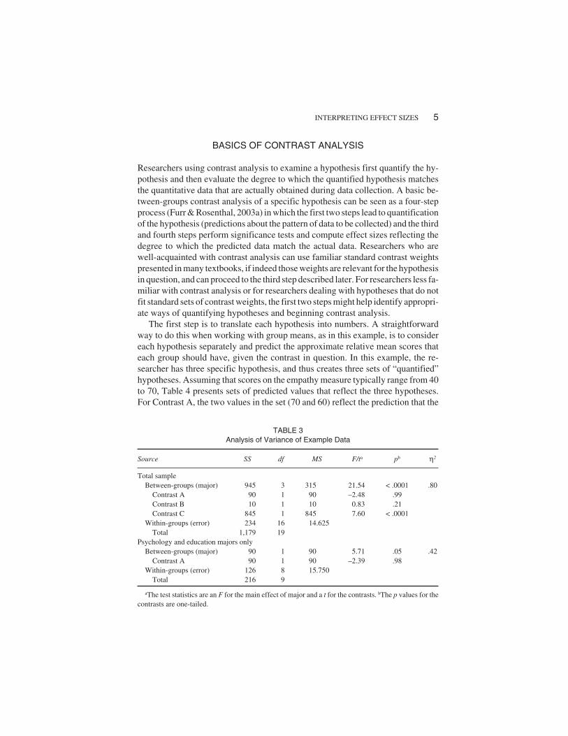
dom, is significant at p < .05, and accounts for 80% of the total variation in empathyscores, as shown by the ANOVA results presented in Table 3. Furthermore, imag-ine that, on the basis of theoretical predictions, the researcher is interested in threespecific hypotheses:

Contrast A: Psychology majors have higher empathy scores than Educationmajors.

Contrast B: Business majors have higher empathy scores than Chemistry majors.Contrast C: On average, Psychology and Education majors have higher empa-

thy scores than Business and Chemistry majors.

In this case, the three contrasts are orthogonal (i.e., independent) and com-pletely account for the between-groups effect. The independence andexhaustiveness is reflected in the fact that the sums of squares for the three con-trasts sum to the sum of squares for the main effect of Major (SSA + SSB + SSC =SSBetween; see Table 3 for the ANOVA results associated with each contrast). Whenresearchers examine a set of independent and exhaustive contrasts, they will fullyaccount for all between-groups variation. That is, the between-groups variationwill be completely partitioned among the contrasts. However, it is not necessarythat researchers use multiple contrasts in the analysis of a given data set, nor is itnecessary that multiple contrasts (if they are used) be orthogonal. The logic and in-terpretation remains the same, even though the effect sizes might be calculated inslightly different ways. The contrasts used in a given set of analysis should primar-ily depend on the researcher’s goals and theoretical questions. To more fully un-derstand the effect sizes associated with contrast analysis and the results presentedin Table 3, some background on contrast analysis is necessary.

4 FURR

TABLE 2Example Data

Major

Psychology Education Business Chemistry

Participant Empathy Participant Empathy Participant Empathy Participant Empathy

1 51 6 62 11 50 16 502 56 7 67 12 49 17 453 61 8 57 13 47 18 404 58 9 65 14 45 19 495 54 10 59 15 44 20 41M 56 62 47 45Variance 14.5 17 6.5 20.5

Note. Grand M = 52.5.

BASICS OF CONTRAST ANALYSIS

Researchers using contrast analysis to examine a hypothesis first quantify the hy-pothesis and then evaluate the degree to which the quantified hypothesis matchesthe quantitative data that are actually obtained during data collection. A basic be-tween-groups contrast analysis of a specific hypothesis can be seen as a four-stepprocess (Furr & Rosenthal, 2003a) in which the first two steps lead to quantificationof the hypothesis (predictions about the pattern of data to be collected) and the thirdand fourth steps perform significance tests and compute effect sizes reflecting thedegree to which the predicted data match the actual data. Researchers who arewell-acquainted with contrast analysis can use familiar standard contrast weightspresented in many textbooks, if indeed those weights are relevant for the hypothesisin question, and can proceed to the third step described later. For researchers less fa-miliar with contrast analysis or for researchers dealing with hypotheses that do notfit standard sets of contrast weights, the first two steps might help identify appropri-ate ways of quantifying hypotheses and beginning contrast analysis.

The first step is to translate each hypothesis into numbers. A straightforwardway to do this when working with group means, as in this example, is to considereach hypothesis separately and predict the approximate relative mean scores thateach group should have, given the contrast in question. In this example, the re-searcher has three specific hypothesis, and thus creates three sets of “quantified”hypotheses. Assuming that scores on the empathy measure typically range from 40to 70, Table 4 presents sets of predicted values that reflect the three hypotheses.For Contrast A, the two values in the set (70 and 60) reflect the prediction that the


TABLE 3Analysis of Variance of Example Data

Source SS df MS F/ta pb η2

Total sampleBetween-groups (major) 945 3 315 21.54 < .0001 .80

Contrast A 90 1 90 –2.48 .99Contrast B 10 1 10 0.83 .21Contrast C 845 1 845 7.60 < .0001

Within-groups (error) 234 16 14.625Total 1,179 19

Psychology and education majors onlyBetween-groups (major) 90 1 90 5.71 .05 .42

Contrast A 90 1 90 –2.39 .98Within-groups (error) 126 8 15.750

Total 216 9

aThe test statistics are an F for the main effect of major and a t for the contrasts. bThe p values for thecontrasts are one-tailed.

Psychology group will have a higher mean empathy score than the Educationgroup. Note that the other two groups are irrelevant to this contrast. For Contrast B,the two values (50 and 40) reflect the prediction that the Business group will have ahigher mean empathy score than the Chemistry group. For Contrast C, the four val-ues (65, 65, 45, and 45) reflect the prediction that the Psychology and Educationstudents will have a higher mean than the Business and Chemistry students. Be-cause Contrast C does not differentiate between the Psychology and Educationstudents, both groups are given the same predicted mean (65), as are the Businessand Chemistry students (45). The real goal in this step is, for each hypothesis sepa-rately, to identify which group or groups are predicted to have relatively highermeans than other groups.

The second step is to translate each quantified hypothesis into a set of contrastweights (λs). This can be accomplished by computing the mean of the predictedvalues for a given contrast and subtracting this mean from each of the predictedvalues associated with the contrast. For Contrast A, the mean is 65, so the contrastweights for the Psychology and Education groups could be 5 and –5 respectively.Analyses are simplified when contrast weights are the smallest whole numbersthat could represent the theory. For Contrast A, the researcher could divide thecontrast weights by 5 to obtain weights of +1 and –1. This transformation simpli-fies computations but has no impact on the resulting p values or effect sizes. Thisprocedure retains the predicted pattern and ensures that the weights for a givencontrast sum to zero. Table 4 presents weights associated with each of the threecontrasts.2

6 FURR

TABLE 4Creating Weights for Contrasts A, B, and C

Predicted Means Contrast Weights (λs)

Major Contrast A Contrast B Contrast C Contrast A Contrast B Contrast C

Psychology 70 65 +1 +1Education 60 65 –1 +1Business 50 45 +1 –1Chemistry 40 45 –1 –1

2Although the contrast analyses in this illustration are relatively simple, these two steps are entirelyapplicable to even more complex contrast analyses. For example, a “trend analysis” could evaluate thespecific hypothesis that the psychology students have a larger mean than the education students, who inturn have a larger mean than the business students, who have a larger mean than the chemistry students.A researcher testing this hypothesis could use the predicted values of 70, 60, 50, and 40, respectively,all in a single set, which would be transformed to contrast weights of 3, 1, –1, and –3 respectively. Simi-larly, the procedures could be used in cases in which there are an uneven number of groups. For exam-ple, a researcher could test the hypothesis that psychology and education students will have a largermean than business, chemistry, and dance students. One way of setting up this prediction would be to

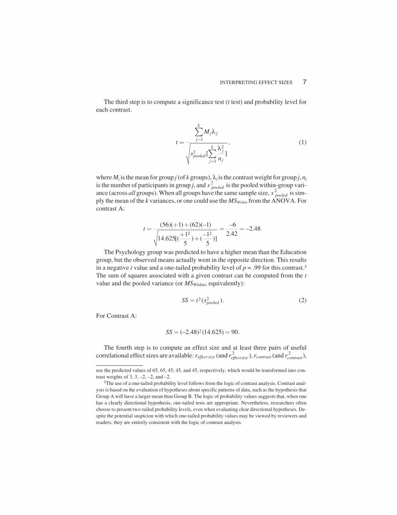
The third step is to compute a significance test (t test) and probability level foreach contrast.

(1)

where Mj is the mean for group j (of k groups), λj is the contrast weight for group j, nj

is the number of participants in group j, and s pooled2 is the pooled within-group vari-

ance (across all groups). When all groups have the same sample size, s pooled2 is sim-

ply the mean of the k variances, or one could use the MSWithin from the ANOVA. Forcontrast A:

The Psychology group was predicted to have a higher mean than the Educationgroup, but the observed means actually went in the opposite direction. This resultsin a negative t value and a one-tailed probability level of p = .99 for this contrast.3

The sum of squares associated with a given contrast can be computed from the tvalue and the pooled variance (or MSWithin, equivalently):

(2)

For Contrast A:

The fourth step is to compute an effect size and at least three pairs of usefulcorrelational effect sizes are available: reffect size (and reffectsize

2 ), rcontrast (and rcontrast2 ),


use the predicted values of 65, 65, 45, 45, and 45, respectively, which would be transformed into con-trast weights of 3, 3, –2, –2, and –2.

3The use of a one-tailed probability level follows from the logic of contrast analysis. Contrast anal-ysis is based on the evaluation of hypotheses about specific patterns of data, such as the hypothesis thatGroup A will have a larger mean than Group B. The logic of probability values suggests that, when onehas a clearly directional hypothesis, one-tailed tests are appropriate. Nevertheless, researchers oftenchoose to present two-tailed probability levels, even when evaluating clear directional hypotheses. De-spite the potential suspicion with which one-tailed probability values may be viewed by reviewers andreaders, they are entirely consistent with the logic of contrast analysis.

1

22

1

,

[ ]

k

j jj

kj

pooledjj

M

t

sn

λ

λ�

�

�

�

�

2 2

(56)( 1) (62)(–1) –6–2.48.

2.421 –114.625[( ) ( )]

5 5

t� �

� � ��

�

22 ( ).pooledSS t s�

2(–2.48) (14.625) 90.SS � �

and ralerting (and ralerting2 ). All three pairs reflect different kinds of effects and are po-

tentially quite useful. The following sections of this article articulate and illustratetheir logic and meanings. The three “unsquared” effect sizes are described and illus-trated, then the three “squared” effect sizes are discussed, and finally the conver-gence with regression is presented.

“UNSQUARED” EFFECT SIZES:CORRELATIONS BETWEEN OBSERVEDAND PREDICTED PATTERNS OF DATA

As just outlined, the weights associated with a given contrast are essentially a quan-tification of the predicted pattern of data, based on theory or prior research. Accord-ingly, “unsquared” effect sizes reflect the degree to which observed data match(i.e., are correlated with) the predicted pattern of data. Each of the three contrastanalysis effect sizes is associated with a different form of the observed data. See Ta-ble 5 for a summary of the unsquared effect sizes for each of the three contrasts.

reffect size

Perhaps the most straightforward effect size for a contrast is reffect size, which is thecorrelation between individuals’ observed scores and the contrast weights that re-flect the predicted pattern of data. Table 6 presents the data in a way that might illus-trate this most clearly for Contrast A. Each participant has two scores: (a) the per-son’s observed empathy score and (b) the contrast weight associated with his or herMajor, as defined for the Contrast A (see Table 4). The reffect size is the correlation be-tween the two sets of scores.

For Contrast A, focusing only on the Psychology and Education students, wetemporarily ignore, or set aside, the Business and Chemistry majors (see the tophalf of Table 6). The correlation between the empathy scores and the contrast

8 FURR

TABLE 5Summary of Effect Sizes for Contrasts A, B, and C

Contrast reffect size ralerting rcontrast

Setting aside irrelevant groupsContrast A –.65 –1.00 –.65 .42 1.00 .42Contrast B .29 1.00 .29 .08 1.00 .08

Including all groupsContrast A –.28 –.31 –.53 .08 .10 .28Contrast B .09 .10 .20 .01 .01 .04Contrast C .85 .95 .88 .72 .89 .78

2effect sizer 2

alertingr 2contrastr

TABLE 6Illustration of Unsquared Effect Sizes for Contrast A

reffect size ralerting rcontrast

Participant EmpathyContrastWeight Major

MEmpathy

ContrastWeight Participant

AdjustedEmpathy

ContrastWeight

Setting aside business and chemistry majors1 51 +1 Psy 56 +1 1 51 +12 56 +1 Edu 62 –1 2 56 +13 61 +1 3 61 +14 58 +1 4 58 +15 54 +1 5 54 +16 62 –1 6 62 –17 67 –1 7 67 –18 57 –1 8 57 –19 65 –1 9 65 –1

10 59 –1 10 59 –1Including business and chemistry majors

1 51 +1 Psy 56 +1 1 44.5 +12 56 +1 Edu 62 –1 2 49.5 +13 61 +1 Bus 47 0 3 54.5 +14 58 +1 Che 45 0 4 51.5 +15 54 +1 5 47.5 +16 62 –1 6 55.5 –17 67 –1 7 60.5 –18 57 –1 8 50.5 –19 65 –1 9 58.5 –1

10 59 –1 10 42.5 –111 50 0 11 55.5 012 49 0 12 54.5 013 47 0 13 52.5 014 45 0 14 50.5 015 44 0 15 49.5 016 50 0 16 57.5 017 45 0 17 52.5 018 40 0 18 47.5 019 49 0 19 56.5 020 41 0 20 48.5 0

Note. Psy = psychology; Edu = education; Bus = business; Che = chemistry.

9

weights for the 10 Psychology and Education students, reffect size = –.65. The corre-lation is negative because the Psychology mean score was lower than the Educa-tion mean score, which contradicts predictions. Instead of computing thecorrelation directly, researchers could obtain this reffect size from the ANOVA of thedata from only the groups involved in the contrast (the bottom half of Table 3 pres-ents the ANOVA results for only the Psychology and Education students):

(3)

where t is the t value associated with the contrast (see Equation 1), FBetween and dfBe-

tween are from the main effect of major in the ANOVA, and dfWithin is from the errorterm in the ANOVA.4 For Contrast A:

Researchers using this formula must be aware of the appropriate sign of the effectsize.

In some cases, the researcher might choose to include the Business and Chemis-try students in the analysis of Contrast A, rather than setting them aside. For exam-ple, if the researcher actually hypothesized that the Business and Chemistrystudents’ empathy scores would fall in between the Psychology and Education stu-dents’ scores, or if the researcher wished to put the contrast in the context of the to-tal variation in the whole sample, then he or she would compute reffect size using theempathy scores and contrast weights for all 20 participants (reffect size = –.28). Or,the researcher could use Equation 3, but use the t value and FBetween from theANOVA conducted on the whole sample:

The procedure that includes all participants has a nice convergence with the re-sults of the full ANOVA and this convergence will be discussed in more detail inthe section on squared effect sizes.

10 FURR

2,

( )effect size

Between Between Within

tr

F df df�

�

2(–2.39).65 –.65.

5.714(1) 8effect sizer � � �

�

2(–2.48).28 –.28.

21.54(3) 16effect sizer � � �

�

4Although the logic and interpretation is exactly the same, a technical consideration is the possibil-ity of using the error term from the ANOVA conducted on the whole sample because it is based on moreobservations and thus would be considered a better estimate of the population error term. In this case,the t value for Contrast A = –2.48, FBetween = 6.15, and reffect size = –.66.

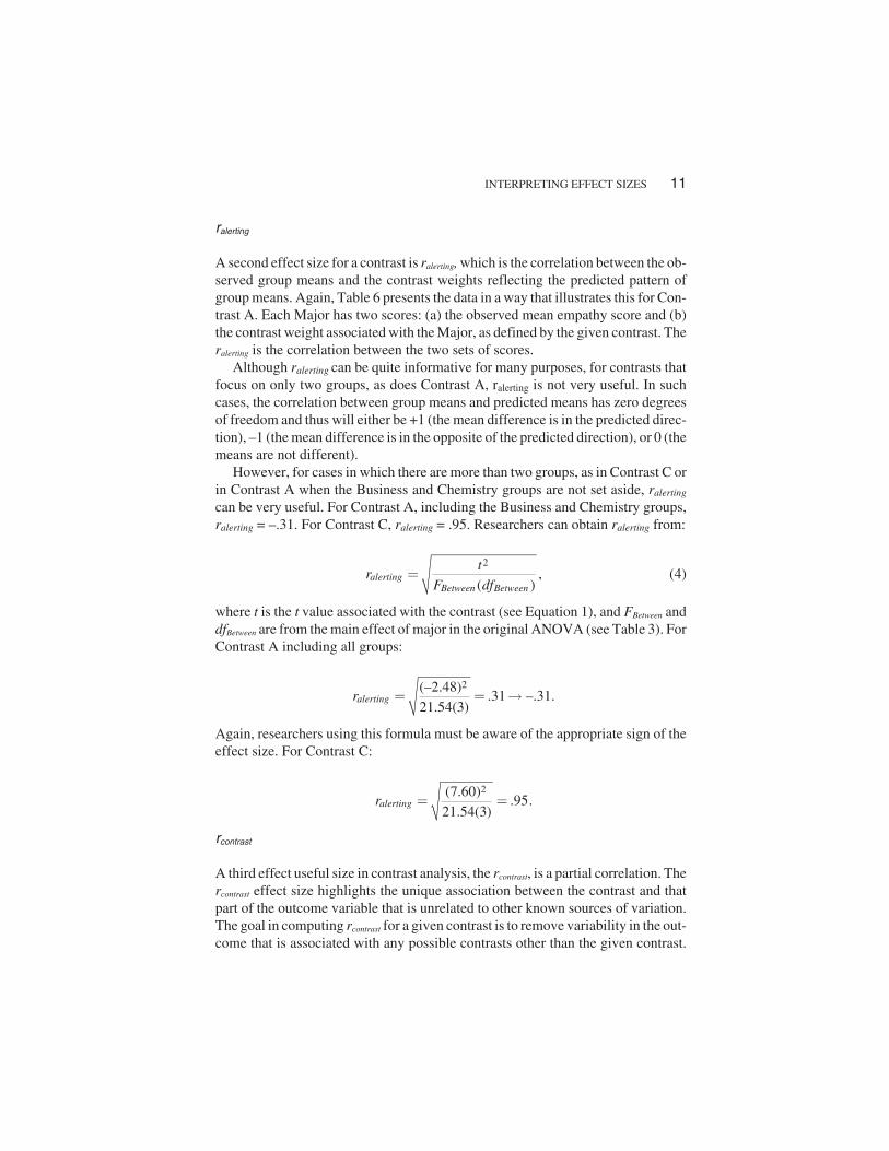
ralerting

A second effect size for a contrast is ralerting, which is the correlation between the ob-served group means and the contrast weights reflecting the predicted pattern ofgroup means. Again, Table 6 presents the data in a way that illustrates this for Con-trast A. Each Major has two scores: (a) the observed mean empathy score and (b)the contrast weight associated with the Major, as defined by the given contrast. Theralerting is the correlation between the two sets of scores.

Although ralerting can be quite informative for many purposes, for contrasts thatfocus on only two groups, as does Contrast A, ralerting is not very useful. In suchcases, the correlation between group means and predicted means has zero degreesof freedom and thus will either be +1 (the mean difference is in the predicted direc-tion), –1 (the mean difference is in the opposite of the predicted direction), or 0 (themeans are not different).

However, for cases in which there are more than two groups, as in Contrast C orin Contrast A when the Business and Chemistry groups are not set aside, ralerting

can be very useful. For Contrast A, including the Business and Chemistry groups,ralerting = –.31. For Contrast C, ralerting = .95. Researchers can obtain ralerting from:

(4)

where t is the t value associated with the contrast (see Equation 1), and FBetween anddfBetween are from the main effect of major in the original ANOVA (see Table 3). ForContrast A including all groups:

Again, researchers using this formula must be aware of the appropriate sign of theeffect size. For Contrast C:

rcontrast

A third effect useful size in contrast analysis, the rcontrast, is a partial correlation. Thercontrast effect size highlights the unique association between the contrast and thatpart of the outcome variable that is unrelated to other known sources of variation.The goal in computing rcontrast for a given contrast is to remove variability in the out-come that is associated with any possible contrasts other than the given contrast.


2,

( )alerting

Between Between

tr

F df�

2(–2.48).31 –.31.

21.54(3)alertingr � � �

2(7.60).95.

21.54(3)alertingr � �

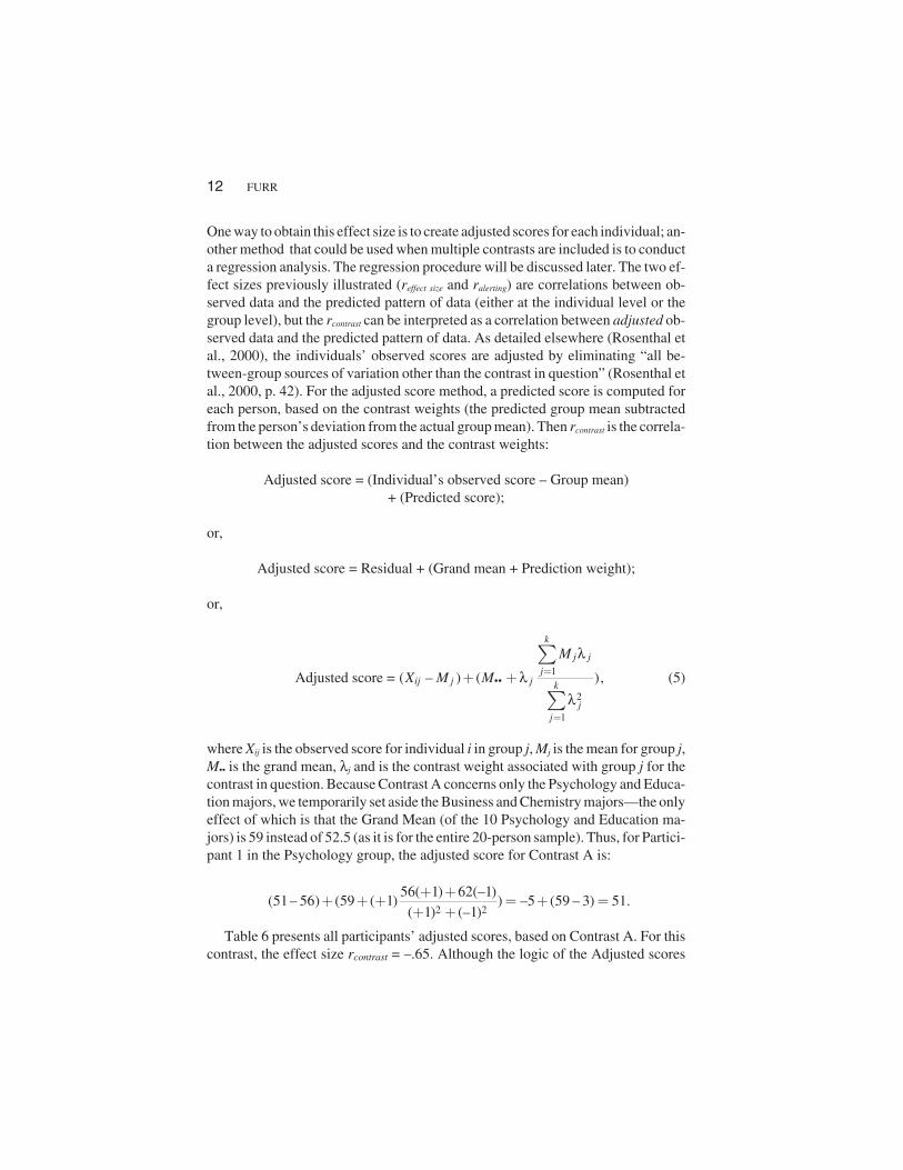
One way to obtain this effect size is to create adjusted scores for each individual; an-other method that could be used when multiple contrasts are included is to conducta regression analysis. The regression procedure will be discussed later. The two ef-fect sizes previously illustrated (reffect size and ralerting) are correlations between ob-served data and the predicted pattern of data (either at the individual level or thegroup level), but the rcontrast can be interpreted as a correlation between adjusted ob-served data and the predicted pattern of data. As detailed elsewhere (Rosenthal etal., 2000), the individuals’ observed scores are adjusted by eliminating “all be-tween-group sources of variation other than the contrast in question” (Rosenthal etal., 2000, p. 42). For the adjusted score method, a predicted score is computed foreach person, based on the contrast weights (the predicted group mean subtractedfrom the person’s deviation from the actual group mean). Then rcontrast is the correla-tion between the adjusted scores and the contrast weights:

Adjusted score = (Individual’s observed score – Group mean)+ (Predicted score);

or,

Adjusted score = Residual + (Grand mean + Prediction weight);

or,

(5)

where Xij is the observed score for individual i in group j, Mj is the mean for group j,M•• is the grand mean, λj and is the contrast weight associated with group j for thecontrast in question. Because Contrast A concerns only the Psychology and Educa-tion majors, we temporarily set aside the Business and Chemistry majors—the onlyeffect of which is that the Grand Mean (of the 10 Psychology and Education ma-jors) is 59 instead of 52.5 (as it is for the entire 20-person sample). Thus, for Partici-pant 1 in the Psychology group, the adjusted score for Contrast A is:

Table 6 presents all participants’ adjusted scores, based on Contrast A. For thiscontrast, the effect size rcontrast = –.65. Although the logic of the Adjusted scores

12 FURR

1••

2

1

Adjusted score = ( – ) ( ),

k

j j

jij j j k

jj

M

X M M

λλ

λ

�

�

� �

�

�

2 2

56( 1) 62(–1)(51– 56) (59 ( 1) ) –5 (59 – 3) 51.

( 1) (–1)� �

� � � � � ��

helps reveal the meaning of the rcontrast effect size, the procedure is obviously un-wieldy and researchers can compute the value more easily from:

(6)

In the current data:

Note that for Contrast A, the rcontrast computed when the Business and Chemis-try students are set aside is equivalent to the reffect size. This is because, by focusingonly on two groups, there is no between-groups variation other than the variationbetween the two groups, thus nothing is partialled when rcontrast is computed in thiscase. In cases in which other between-groups variation (apart from the contrast inquestion) does exist, rcontrast and reffect size lead to importantly different results. Forexample, if we compute rcontrast for Contrast A, without setting aside the Businessand Chemistry majors, we obtain rcontrast = –.53. Similarly, if we compute rcontrast

for Contrast C, we obtain rcontrast = .88.

“SQUARED” EFFECT SIZES:“PROPORTION OF VARIATION ACCOUNTED FOR”

Many researchers may be more familiar with interpreting effect sizes as “propor-tion of variance accounted for” than as the degree of relation between predicted andobserved data. For example, R2 (from regression) and η 2 (from ANOVA) are popu-lar effect sizes reflecting the proportion of total variation in scores on a dependentvariable that is accounted for by variation on some predictor variable or set of pre-dictor variables. An understanding of the effect sizes associated with contrast anal-ysis might be facilitated by thinking of the ANOVA between-groups sums ofsquares (SSBetween in Table 3) as “explained” variation and thinking of the error orwithin-groups sums of squares (SSWithin in Table 3) as “unexplained” variation.

From the ANOVA of the data in Table 2, SSTotal represents the degree to whichall 20 students’ empathy scores differ from each other and SSBetween represents thedifferences among the 20 empathy scores that are associated with the fact thatsome majors tend to have higher empathy scores than other majors. So the meanempathy score differences between majors accounts for, or explains, some amountof the total differences among the individual students. As a matter of fact, the factthat some majors seem to have generally higher empathy scores than others ex-plains 80% of the total variation in empathy:


2

2.contrast

Within

tr

t df�

�

2

2

–2.39.65 –.65.

–2.39 8contrastr � � �

�

Note that, at this point, this is a rather vague form of “explained”—yes, somegroups are different from others, but the nature of the between-groups differencesremains to be explored. For example, which groups are different from which? Arethe differences between some groups bigger than the differences between others?Contrast analyses reveal these more specific facets of the general between-groups“explanation.”

SSWithin represents the variation among empathy scores that is not explainableby differences between majors. For example, Allen and Beth are both Psychologymajors, but Allen has a lower empathy score than Beth. Because they are both inthe same major, the difference between the two participants’ scores is“within-major” variation, which is unrelated to (and thus not explainable by) thefact that different majors tend to have different scores. There could be meaningfulreasons why Allen and Beth have different empathy levels—maybe there are gen-der differences or perhaps intelligence is related to empathy. However, those po-tential explanations are not included in the current analyses, so the within-majorvariation is left unexplained.

SSContrast for a given contrast represents the variation among empathy scoresthat is explained by that particular contrast. For example, as Table 3 shows, thesums of squares associated with Contrast A is 90—this is the “piece” of the ex-plained empathy variation that is specifically explained by the average differencebetween Psychology and Education majors. Each of the squared effect sizes asso-ciated with contrasts identifies the “proportion of variation” in relation to differentpieces of the variation.

Again, perhaps the most straightforward and familiar effect size for a given contrastis reffectsize

2 , which can be interpreted as the proportion of total variation that is ex-plained by the contrast:

or,

14 FURR

2effect sizer

2 The piece of the variation explained by the given contrast,

Total variationeffect sizer �

2 ,Piece of the explainedeffect size

Explained Unexplained

SSr

SS SS�

�

2

945.80

1179(this is from the overall ANOVA).

Between Between

Total Between Within

SS SS

SS SS SSη

� � ��

or,

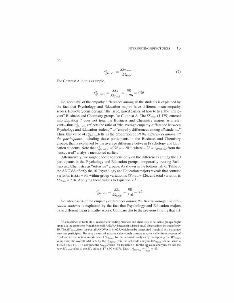
(7)

For Contrast A in this example,

So, about 8% of the empathy differences among all the students is explained bythe fact that Psychology and Education majors have different mean empathyscores. However, consider again the issue, raised earlier, of how to treat the “irrele-vant” Business and Chemistry groups for Contrast A. The SSTotal (1,179) enteredinto Equation 7 does not treat the Business and Chemistry majors as irrele-vant—thus reffectsize

2 reflects the ratio of “the average empathy difference betweenPsychology and Education students” to “empathy differences among all students.”Thus, this value of reffectsize

2 tells us the proportion of all the differences among allthe participants, including those participants in the Business and Chemistrygroups, that is explained by the average difference between Psychology and Edu-cation students. Note that reffectsize

2 2076 28= =. –. , where –.28 = reffect size from the“unsquared” analysis mentioned earlier.

Alternatively, we might choose to focus only on the differences among the 10participants in the Psychology and Education groups, temporarily treating Busi-ness and Chemistry as “set-aside” groups. As shown in the bottom half of Table 3,the ANOVA of only the 10 Psychology and Education majors reveals that contrastvariation is SSA = 90, within-group variation is SSWithin = 126, and total variation isSSTotal = 216. Applying these values to Equation 7,5

So, about 42% of the empathy differences among the 10 Psychology and Edu-cation students is explained by the fact that Psychology and Education majorshave different mean empathy scores. Compare this to the previous finding that 8%


2 90.076.

1179A

effect sizeTotal

SSr

SS� � �

5As described in footnote 4, researchers treating business and chemistry as set-aside groups mightopt to use the error term from the overall ANOVA because it is based on 20 observations instead of only10. The MSWithin from the overall ANOVA is 14.625, which can be interpreted (roughly) as the averageerror per participant. Because a sums of squares value equals a mean squares value times degrees offreedom, we can obtain an estimate of SSWithin for the set-aside analysis by multiplying the MSWithin

value from the overall ANOVA by the dfWithin from the set-aside analysis (SSWithin for set aside =14.625 × 8 = 117). To compute the SSTotal value (for Equation 6) for the set-aside analysis, we add thenew SSWithin value to the SSA value (117 + 90 = 207). Thus, .2 90

.43207effect sizer � �

2 90.42.

216A

effect sizeTotal

SSr

SS� � �

2 .Contrasteffect size

Total

SSr

SS�

of the empathy differences among all 20 students are explained by the fact thatPsychology and Education majors have different mean empathy scores. Decidingwhich one of these effect sizes (treating Business and Chemistry as set-asidegroups or not) is appropriate depends on the question that a researcher wishes toanswer. Researchers might even choose to report both versions of reffectsize

2 .

The second squared effect size, ralerting2 , is also relatively straightforward, and can

be interpreted as the proportion of the explained variation that is explained by thecontrast:

or,

or,

(8)

For Contrast A in this example,

So, about 10% of the variation in mean empathy differences among all fourgroups is explained by the fact that Psychology and Education majors have differ-ent mean empathy scores. This value, although informative, may not exactly re-flect the spirit of Contrast A, for which the Business and Chemistry majors couldbe considered irrelevant. Alternatively, the researcher could again focus only onthe ANOVA for the 10 Psychology and Education majors. However such an analy-sis would be pointless in this context—it would tell the researcher that 100% of thevariation in mean empathy differences among the Psychology group and the Edu-cation group is explained by the fact that Psychology and Education majors havedifferent mean empathy scores. That is, the Contrast A is all of the between-groupsvariation, when the Business and Chemistry groups are set aside.

Contrast C provides a good illustration of the usefulness of ralerting2 . In this case,

there are no irrelevant groups, so for Contrast C:

16 FURR

2alertingr


All explained variationalertingr �

2 ,Pieceof theexplainedalerting

Explained

SSr

SS�

2 .Contrastalerting

Between

SSr

SS�

2 90.095.

945A

alertingBetween

SSr

SS� � �

This value shows “where the action is” in the differences between groups. Spe-cifically, it tells us that 89% of the variation among the four groups arises from thefact that Psychology and Education majors have a larger mean empathy score thando Business and Chemistry majors.

One way to approach the rcontrast2 effect size is to consider it in light of the other

two squared effect sizes. The reffectsize2 reflects the proportion of the total varia-

tion that is explained by a particular contrast and the ralerting2 reflects the propor-

tion of the explained variation that is explained by a particular contrast. Thercontrast

2 effect size can be seen as a way of expressing the particular contrast inrelation to the unexplained variation, or the variation that is unexplained by anyother contrasts:

or,

or,

or,

(9)

In this example, For Contrast A:


2contrastr


Variation unexplained by any other contrastcontrastr �

2

The piece of the variation explained by the given contrast,

The piece of the variation explained by the given contrast + Unexplained variation

contrastr �

2 ,Pieceof theexplained

Pieceof theexplainedcontrast

Unexplained

SSr

SS SS�

�

2 .Contrastcontrast

Contrast Within

SSr

SS SS�

�

2 90.28.

90 234A

contrastA Within

SSr

SS SS� � �

� �

2 845.89.

945C

alertingBetween

SSr

SS� � �

So, according to the rcontrast2 for Contrast A, the mean empathy difference be-

tween Psychology and Education students accounts for 28% of the variation in em-pathy among all 20 students that is unrelated to all other between-group contrasts.That is, rcontrast

2 Contrast A accounts for 28% of the variation in empathy that is leftover after all other between-group contrasts have been taken into consideration(“removed”). Or, put yet another way, it accounts for 28% of the variation in em-pathy that is related to the combination of mean differences between Psychologyand Education students and of Unexplained variation. As seen with the unsquaredeffect sizes illustrated earlier, if Business and Chemistry majors are set aside, thenrcontrast

2 is equivalent to reffectsize2 .

To summarize the squared effect sizes, the differences lie in the denominatorsof the formulae (illustrated with regard to Contrast A):

CONVERGENCE BETWEEN CONTRAST EFFECT SIZESAND MULTIPLE REGRESSION

Some researchers might find the connection between the contrast effect sizes andmultiple regression analysis to be particularly revealing. Cohen (1968) pointed outthat many ANOVA procedures can be performed fruitfully as multiple regressionanalysis, and contrast analysis is no exception. The “effect size” and “contrast” ef-fect sizes have direct parallels to the output of typical regression analysis that fo-cuses on individual-level data. Because the “alerting” effect size is at the grouplevel, instead of the person level, it could be integrated with the other two effectsizes within a multilevel modeling (or hierarchical linear modeling) approach.

Imagine that the researcher conducts a regression analysis predicting individu-als’ scores on empathy from three variables reflecting Contrasts A, B, and C (seeTable 7 for the likely data structure for such an analysis). The squared zero-ordercorrelation for a predictor contrast (or its squared semi-partial correlation in thisexample because all the contrasts are orthogonal) for a predictor is equivalent to

18 FURR

2

90 90.076,

90 10 845 234 1,179

A Aeffect size

A B C Within Between Within

SS SSr

SS SS SS SS SS SS� �

� � � �

� � ��

2 90 90.095,

90 10 845 945A A

alertingA B C Between

SS SSr

SS SS SS SS� � � � �

� � � �

2 90 90.278.

90 234 324A

contrastA Within

SSr

SS SS� � � �

� �

reffectsize2 , and the squared partial correlation for a predictor contrast is equivalent to

rcontrast2 . A partial correlation for a particular predictor is the correlation between

that portion of the outcome that is unrelated to all other predictors and that portionof the predictor that is unrelated to all other predictors. That is, the other predictorsare partialled from the focal predictor and from the outcome variable. For ContrastA in this example, the partial correlation is the correlation between that part of em-pathy that is unrelated to Contrast B and C, and that part of Contrast A that is unre-lated to Contrast B and C. In cases where all contrasts are orthogonal, as in thisexample, each contrast is inherently unrelated to all other contrasts.

As shown in Figure 1, contrast analysis and the reffectsize2 , ralerting

2 , and rcontrast2 ef-

fect sizes can be expressed through a Venn diagram (e.g., Cohen & Cohen, 1983,p. 89), which might reveal the convergence with regression the “proportion ofvariation accounted for” interpretation even more clearly. Each contrast variable isrepresented by a circle, as is empathy. Each of the three contrasts explains, or is as-sociated with, a separate part of empathy, which arises from the orthogonality ofthe three contrasts. In other words, each piece of variation explained by the threecontrasts is “unique” variation. For example, the “a” portion of the diagram is thatpart of empathy uniquely explained by Contrast A, and the total variation in empa-thy is (a + b + c + d). Thus, for Contrast A:


TABLE 7Data for Regression Analysis of Contrasts A, B, and C

Participant Empathy Contrast A Contrast B Contrast C

1 51 +1 0 +12 56 +1 0 +13 61 +1 0 +14 58 +1 0 +15 54 +1 0 +16 62 –1 0 +17 67 –1 0 +18 57 –1 0 +19 65 –1 0 +1

10 59 –1 0 +111 50 0 +1 –112 49 0 +1 –113 47 0 +1 –114 45 0 +1 –115 44 0 +1 –116 50 0 –1 –117 45 0 –1 –118 40 0 –1 –119 49 0 –1 –120 41 0 –1 –1

CONCLUSIONS

Effect sizes are becoming increasingly integrated into and expected as part of statis-tical analysis in the social sciences. Many effect sizes are available to researchers,but many discussions of effect sizes are long on computation and rather short on in-terpretation. Consequently, researchers and reviewers could be forgiven for beingsomewhat unclear about the exact meaning of a given effect size or of the differencebetween effect sizes. This article is intended to help articulate and clarify the mean-ing of three correlational effect sizes associated with contrast analysis.

Because contrast analysis and the effect sizes discussed in this article are but apiece of the large puzzle of understanding one’s data and evaluating one’s theories,a few broader issues merit comment. First, recent recommendations (e.g., Cohen,1990; Loftus, 1996; Wilkinson et al., 1999) highlight the usefulness of exploratorydata analysis, and particularly the graphical presentation of data. Whether used toaid the detection of problems in the data, such as outliers; to potentially uncoverunforeseen differences or trends, such as quadratic associations; or simply to pres-ent data in a clear and efficient modality, graphical examination of data might pre-

20 FURR

FIGURE 1 Venn diagram for effect sizes in contrast analysis.

2

2

2

squared correlation

r squared partial correlation

no direct parallel in multiple regression

at the individual level .

effect size

contrast

alerting

ar

a b c da

a da

ra b c

� ��

� ��

� ��

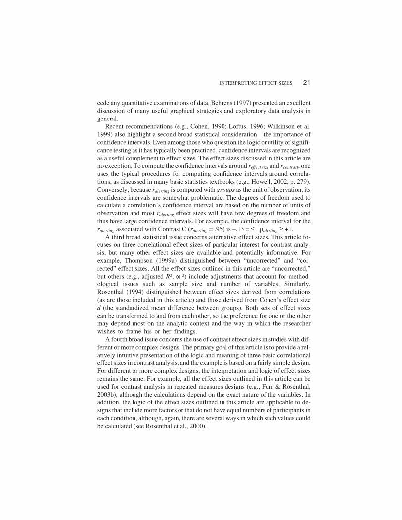
cede any quantitative examinations of data. Behrens (1997) presented an excellentdiscussion of many useful graphical strategies and exploratory data analysis ingeneral.

Recent recommendations (e.g., Cohen, 1990; Loftus, 1996; Wilkinson et al.1999) also highlight a second broad statistical consideration—the importance ofconfidence intervals. Even among those who question the logic or utility of signifi-cance testing as it has typically been practiced, confidence intervals are recognizedas a useful complement to effect sizes. The effect sizes discussed in this article areno exception. To compute the confidence intervals around reffect size and rcontrast, oneuses the typical procedures for computing confidence intervals around correla-tions, as discussed in many basic statistics textbooks (e.g., Howell, 2002, p. 279).Conversely, because ralerting is computed with groups as the unit of observation, itsconfidence intervals are somewhat problematic. The degrees of freedom used tocalculate a correlation’s confidence interval are based on the number of units ofobservation and most ralerting effect sizes will have few degrees of freedom andthus have large confidence intervals. For example, the confidence interval for theralerting associated with Contrast C (ralerting = .95) is –.13 = ≤ ρalerting ≥ +1.

A third broad statistical issue concerns alternative effect sizes. This article fo-cuses on three correlational effect sizes of particular interest for contrast analy-sis, but many other effect sizes are available and potentially informative. Forexample, Thompson (1999a) distinguished between “uncorrected” and “cor-rected” effect sizes. All the effect sizes outlined in this article are “uncorrected,”but others (e.g., adjusted R2, ω 2) include adjustments that account for method-ological issues such as sample size and number of variables. Similarly,Rosenthal (1994) distinguished between effect sizes derived from correlations(as are those included in this article) and those derived from Cohen’s effect sized (the standardized mean difference between groups). Both sets of effect sizescan be transformed to and from each other, so the preference for one or the othermay depend most on the analytic context and the way in which the researcherwishes to frame his or her findings.

A fourth broad issue concerns the use of contrast effect sizes in studies with dif-ferent or more complex designs. The primary goal of this article is to provide a rel-atively intuitive presentation of the logic and meaning of three basic correlationaleffect sizes in contrast analysis, and the example is based on a fairly simple design.For different or more complex designs, the interpretation and logic of effect sizesremains the same. For example, all the effect sizes outlined in this article can beused for contrast analysis in repeated measures designs (e.g., Furr & Rosenthal,2003b), although the calculations depend on the exact nature of the variables. Inaddition, the logic of the effect sizes outlined in this article are applicable to de-signs that include more factors or that do not have equal numbers of participants ineach condition, although, again, there are several ways in which such values couldbe calculated (see Rosenthal et al., 2000).


Differentiating and Using the Effect Sizes

The effect sizes described in this article differ from each other in a number impor-tant ways, and researchers might wonder if some are more preferable than others.The short answer to this question is that the different effect sizes provide answers todifferent questions, so the appropriate effect sizes are the ones that answer the rele-vant analytic questions. In a given analytic situation, a researcher might choose touse several of the effect sizes, recognizing that each provides distinct and poten-tially important information. Nevertheless, the differences among the effect sizesare worth further consideration.

As outlined in this article, a researcher might consider reporting either un-squared or squared effect sizes (or both). If an analytic question seems to be intu-itively framed in terms of “to what degree to the observed data match thepredictions?,” then unsquared effect sizes will be appropriate. For analytic ques-tions more intuitively framed as “to what degree does the contrast account for vari-ation in the data?,” then the squared effect sizes will be more useful. In generalthough, the unsquared approaches might be preferable for at least two reasons.First, they allow researchers to retain information about the direction of the rela-tion. In this article, analysis of Contrast A revealed that the data contradicted thehypothesis and this contradiction is reflected in the sign of the unsquared effectsizes, but is lost in the squared effect sizes. Thus, unsquared effect sizes provide di-rect information about both the magnitude and direction of association betweenpredictions and observations. Second, the unsquared effect sizes avoid the inter-pretational ambiguity and criticisms leveled at squared effect sizes. For example,some researchers have argued that squaring puts the effect sizes on a nonintuitiveand inappropriate metric of variation, that squaring is based on a statistical modelthat is often inappropriate for making conclusions about amount of determination,and that squaring often leads to an underestimation of the importance of effects(Abelson, 1985; D’Andrade & Dart, 1990; Ozer, 1985; Rosenthal & Rubin, 1979).

A second distinction arises when some data could be treated as irrelevant to agiven contrast and thus be set aside. This distinction arises for contrasts that focus ononly some participants or groups, such as Contrasts A and B in these examples; itdoes not arise for contrasts that include all groups, such as Contrast C. So, for con-trasts in which some data could be set aside, which one is correct—the set-aside pro-cedure or the full sample procedure? They are both reasonable and potentiallyuseful, but they differ primarily in terms of which sample is of interest. If researcherswish to focus only on a subsample (e.g., only the differences between the Psychol-ogyandtheEducationmajors), then theset-asideproceduremightbemoreappropri-ate. This might particularly hold true when using a nonsquared effect size (e.g., reffect

size)—when the effect size is to be interpreted as the correlation between observeddata and predicted data. In such cases, the predicted data really only involve a subsetof participants and to include predicted data for the full sample might misrepresent

22 FURR

the meaning of the contrast. Conversely, when using squared effect sizes (e.g.,reffectsize

2 ), both the set-aside and the full-sample analysis could be quite meaningful.For many research situations, it may indeed be reasonable to report the degree towhich a given contrast explains variation within a particular subsample and withinthe full sample. Note that the set-aside effect sizes will always be equal to, or morelikely, greater than, full-sample effect sizes (see Table 5). Finally, if researchers areattempting to represent results with regard to the total sample, then the full-sampleeffect sizes are of course more appropriate than set-aside effect sizes. See Rosenthalet al. (2000, pp. 56–61, 102–112) for a variety of additional considerations about theset-aside strategies.

Aside from the issues of squaring and setting aside, how can the differencesamong the three basic effect sizes—reffect size, ralerting, and rcontrast—be summarized?Both reffect size and ralerting have relatively straightforward interpretations—they arezero-order correlations between observed data and predicted data. In addition, theyboth reflect the degree to which participants in one group (or groups) have a largermean score than participants in another group (or groups). They differ only with re-gard to the level of aggregation. The reffect size analysis is at the level of the individualand thus includes all participants—so individual differences within a group (i.e.,within-group variation or error variation) are included in the analysis. The ralerting

analysis is at the level of the group and thus includes only group means—individualdifferences among the participants within groups are not included in the analysis. Aconsequence of this difference is that reffect size will always be smaller than ralerting (as-suming that there is some degree of within-group variation).

Finally, rcontrast is conducted at the individual level, but is a way of partialling outor controlling for variation associated with other contrasts. The distinction betweenrcontrast and reffect size becomes more apparent when considering the fact that differentresearch designs will likely include different factors, different numbers of factors,and different kinds of participants. The rcontrast effect size describes a particular con-trast in relation to error variation only, whereas reffect size describes a particular con-trast in relation to all variation within a given study. Consider the possibility that tworesearchers each conduct a study of some phenomenon and obtain the same exactrcontrast. However one researcher included a larger number of factors in her study,which increases the total variation in the dependent variable. This would result in thetwo researchers obtaining different (perhaps drastically different) reffect size values.Thus, rcontrast (and rcontrast

2 ) might be particularly useful for comparing contrast anal-yses across studies, and thus would be quite useful as a meta-analytic tool.

The “Size” of Effect Sizes

An additional issue involves concluding whether a given effect size value is “large”or of practical importance. Many researchers have acknowledged that statisticalsignificance, size of effect, and importance of effect are separate issues (e.g.,


Rosnow & Rosenthal, 1989). Although Cohen (1988) provided guidelines forgauging the size of effects, a strict adherence to these guidelines is probably coun-terproductive (Thompson, 1999a). McCartney and Rosenthal (2000) outlined threeconsiderations in interpreting effect size and practical importance. First, an effectshould be considered in the context of methodological issues such as measurementand research design. For example, the measurement technologies in the social sci-ences are generally less precise than those in other sciences and this limits the effectsizes that we are likely to observe. Second, an effect should be considered in thecontext of relevant research literature. Is a given effect relatively larger or smallerthan effects observed in similar research areas? Third, an effect can be presented asa binomial effect size display (BESD; Rosenthal & Rubin, 1982), which translates agiven effect size into a 2 × 2 table of outcomes that is relatively intuitive, particu-larly for nonscientists (see also Rosenthal et al., 2000). The BESD, along with acost-benefit analysis, can begin to reveal the potential practical importance of agiven effect.

In sum, more and more researchers in the social sciences are recognizing theimportance of reporting effect sizes. It is hoped that this article enhances the fre-quency and effectiveness with which effect sizes are used in social science re-search.

ACKNOWLEDGMENT

I thank Robert Rosenthal and Timothy Huelsman for their comments on an earlierversion of this article.

REFERENCES

Abelson, R. P. (1985). A variance explanation paradox: When a little is a lot. Psychological Bulletin, 97,129–133.

American Psychological Association. (2001). Publication manual of the American Psychological Asso-ciation (5th ed.). Washington, DC: Author.

Behrens, J. T. (1997). Principles and procedures of exploratory data analysis. Psychological Methods, 2,131–160.

Cohen, J. (1968). Multiple regression as a general data-analytic system. Psychological Bulletin, 70,426–443.

Cohen, J. (1988). Statistical power analysis for the behavioral sciences (2nd ed). Hillsdale, NJ: Law-rence Erlbaum Associates, Inc.

Cohen, J. (1990). Things I have learned (so far). American Psychologist, 45, 1304–1312.Cohen, J. (1994). The earth is round (p < .05). American Psychologist, 49, 997–1003.Cohen, J., & Cohen, P. (1983). Applied multiple regression/correlation analysis for the behavioral sci-

ences (2nd ed.). Hillsdale, NJ: Lawrence Erlbaum Associates, Inc.

24 FURR

D’Andrade, R., & Dart, J. (1990). The interpretation of r versus r2 or why percentage of variance ac-counted for is a poor measure of size of effect. Journal of Quantitative Anthropology, 2, 47–59.

Furr, R. M., & Rosenthal, R. (2003a). Evaluating theories efficiently: The nuts and bolts of contrast anal-ysis. Understanding Statistics, 2, 45–67.

Furr, R. M., & Rosenthal, R. (2003b). Repeated-measure contrasts for “multiple-pattern” hypotheses.Psychological Methods, 8, 275–293.

Howell, D. C. (2002). Statistical methods for psychology (5th ed.). Belmont, CA: Duxbury.Keselman, H. J., Huberty, C. J., Lix, L. M., Olejnik, S., Cribbie, R., Donahue, B., et al. (1998). Statistical

practices of educational researchers: An analysis of their ANOVA, MANOVA, and ANCOVA anal-yses. Review of Educational Research, 68, 350–386.

Kirk, R. (1996). Practical significance: A concept whose time has come. Educational and PsychologicalMeasurement, 56, 746–759.

Loftus, G. R. (1996). Psychology will be a much better science when we change the way that we analyzedata. Current Directions in Psychological Science, 5, 161–171.

McCartney, K., & Rosenthal, R. (2000). Effect size, practical importance, and social policy for children.Child Development, 71, 173–180.

Ozer, D. J. (1985). Correlation and the coefficient of determination. Psychological Bulletin, 97,307–315.

Rosenthal, R. (1994). Parametric measures of effect size. In H. Cooper & L. V. Hedges (Eds.), The hand-book of research synthesis (pp. 231–244). New York: Sage.

Rosenthal, R., Rosnow, R. L., & Rubin, D. B. (2000). Contrasts and effect sizes in behavioral research:A correlational approach. Cambridge, England: Cambridge University Press.

Rosenthal, R., & Rubin, D. B. (1979). A note on percent of variance explained as a measure of the impor-tance of effects. Journal of Applied Social Psychology, 9, 395–396.

Rosenthal, R., & Rubin, D. B. (1982). A simple, general purpose display of magnitude of experimentaleffect. Journal of Educational Psychology, 74, 166–169.

Rosnow, R. L., & Rosenthal, R. (1989). Statistical procedures and the justification of knowledge in psy-chological science. American Psychologist, 44, 1276–1284.

Thompson, B. (1999a). If statistical significance tests are broke/misused, what practices should supple-ment or replace them? Theory & Psychology, 9, 165–181.

Thompson, B. (1999b). Why “encouraging” effect size reporting isn’t working: The etiology of re-searcher resistance to changing practices. Journal of Psychology, 133, 133–140.

Vacha-Haase, T., Nilsson, J. E., Reetz, D. R., Lance, T. S., & Thompson, B. (2000). Reporting practicesand APA editorial policies regarding statistical significance and effect size. Theory & Psychology,10, 413–425.

Wilkinson, L., & the APA Task Force on Statistical Inference. (1999). Statistical methods in psychologyjournals: Guidelines and explanations. American Psychologist, 54, 594–604.


interpreting effect sizes in contrast...

Documents