international conference ppt

8/7/2019 International Conference PPT

http://slidepdf.com/reader/full/international-conference-ppt 1/22

An Econometric Assessment on

Relational Interaction between HigherEducation and Economic Growth in

India

Nishant Joshi, Assistant Professor, Prestige Institute of Management and

Research, Indore

Dr.R.K.Sharma, Professor and Director , Prestige Institute of Management

and Research, Indore.Neha Joshi, PhD Research Scholar, School of Future Studies, DAVV, Indore.



BEFORE WE MOVE AHEAD



T

he relational interaction between educationand economic growth has been the subject of

public debates, enjoying a wide interest since

the era of Plato. According to Dikens et all.

(2006), Zoega (2003) and Barro (1991), theeducation has a high intrinsic economic value

since the investments in education led to the

formation of human capital, which is one of the cause of economic growth.



Amongst the BRIC countries (i.e. Brazil, India,

China and Russia) successful studies has been

conducted in Brazil and china and the result

amongst the two variables showed that higher

education had a significant impact on theeconomic growth for Brazil and China. But a

similar study in Chile showed no causal

relationship amongst the variables.



Podrecca and Carmeci (2002) analyzed the causality between

education and economic growth using Granger causality, for a

set of 86 countries over the period 1960-1990.T

heir resultsshow that both education investment and the educational

stock had an impact to growth rates, both individually and

jointly with physical capital investment. There is also a reverse

causality that runs from growth to investment in education.

Jaoul (2004) analyzed causality between higher education andeconomic growth in France and Germany in the period before

the Second World War. The obtained results demonstrate that

higher education has an influence on gross domestic product

just for the case of France. For Germany, education does not

appear as a cause of growth. Kui (2006) analyzed the causality

and co-integration between education and GDP, showing that

economy development is the cause of higher education



Hunang, Jin, and Sun (2009) analyzed the

causality between scale evolution of higher

education and economic growth in China,

between 1972 and 2007. The empirical results

show that there is a long-term steadyrelationship between variables of enrollment

in higher education and GDP per capita. For

the analyzed period, with the growth of theeconomy, scale of higher education exhibits an

ascending trend.



Objectives

To analyze the causality between higher

education and economic growth for India.



Hypothesis In the first step of the analysis the stationarity of the variables was to be examined.

If all the variables are stationary I(0), if there is no problem to estimate the

coefficients using the variables with initial specification. However, most of the

main macroeconomic variables are non-stationary, integrated of order higher than

zero. If the series are non-stationary but co-integrated, then the estimation as an

autocorrected model is admissible. If the variables are non-stationary and are not

co-integrated then the specification of variables as differences is necessary.

We used the Augmented Dickey-Fuller test (ADF) to test the existence of unit roots

and to determine the order of integration of the variables. The test was conducted

with and without a time trend. In order to test the co-integration of the analyzed

variables, we used the maximum likelihood estimation method of Johansen and

Juelius (1990, 1995), since the cointegration test procedures of Johansen and

Juselius (1990) can distinguish between the existence of one or more cointegrating

vectors and also generate test statistics with exact distributions (Van den Berg and

Jayanetti 1993);



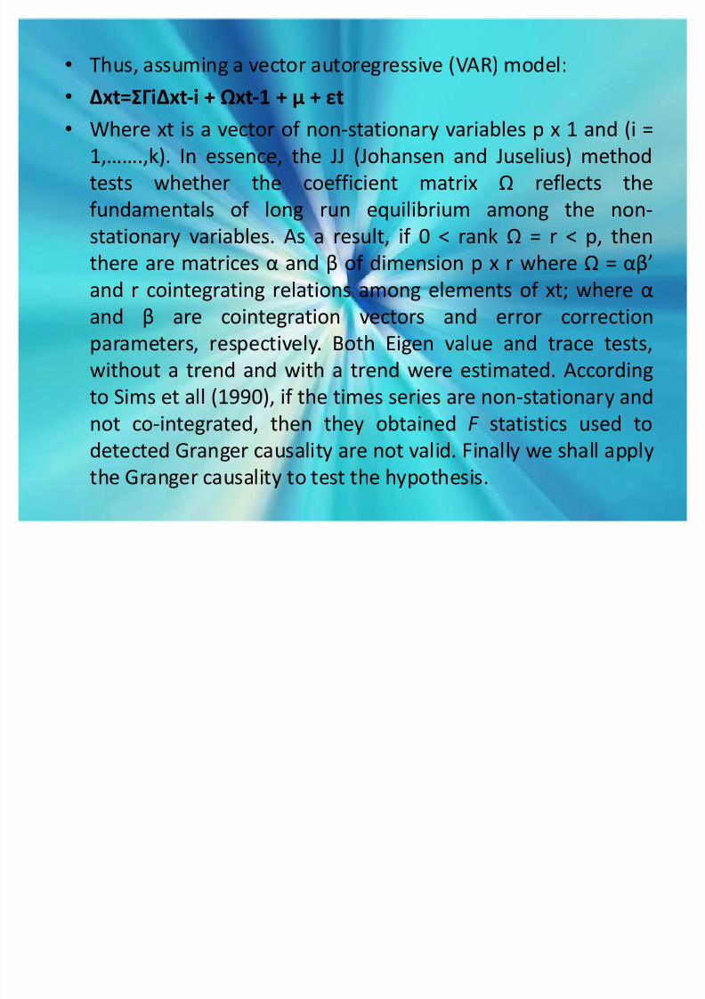
it is hereby appropriate to utilize. Thus, assuming a vector

autoregressive (VAR) model:

xt=ixt-i + xt-1 + + t

Where xt is a vector of non-stationary variables p x 1 and (i =

1,.,k). In essence, the JJ (Johansen and Juselius) method

tests whether the coefficient matrix reflects the

fundamentals of long run equilibrium among the non-stationary variables. As a result, if 0 < rank = r < p, then

there are matrices and of dimension p x r where =

and r cointegrating relations among elements of xt; where

and are cointegration vectors and error correction

parameters, respectively. Both Eigen value and trace tests,without a trend and with a trend were estimated. According

to Sims et all (1990), if the times series are non-stationary and

not co-integrated, then they obtained F statistics used to

detected Granger causality are not valid. Finally we shall applythe Granger causality to test the hypothesis.



Yt = i xt-i + jYt-j + 1t . (1)

Xt = i xt-i + jYt-j + 2t . (2)

with the assumption that the disturbances t1 and t2 are uncorrelated. We distinguish four

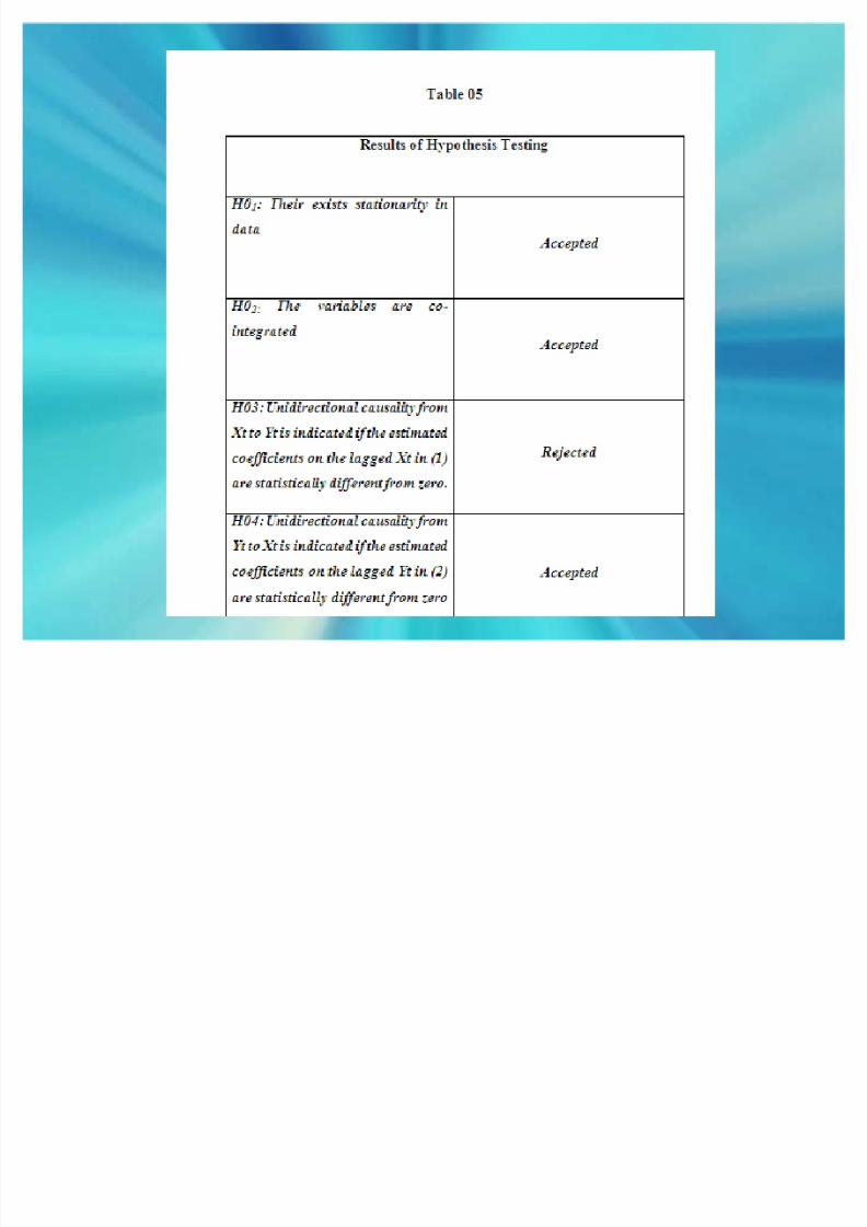
cases: H0 1: Their exists stationarityin data

H0 2: The variables are co-integrated

H0 3: Unidirectional causality from X t to Y t is indicated if the estimated coefficients on the

lagged X t in (1) are statistically different from zero.

H0 4: Unidirectional causality from Y t to X t is indicated if the estimated coefficients on the

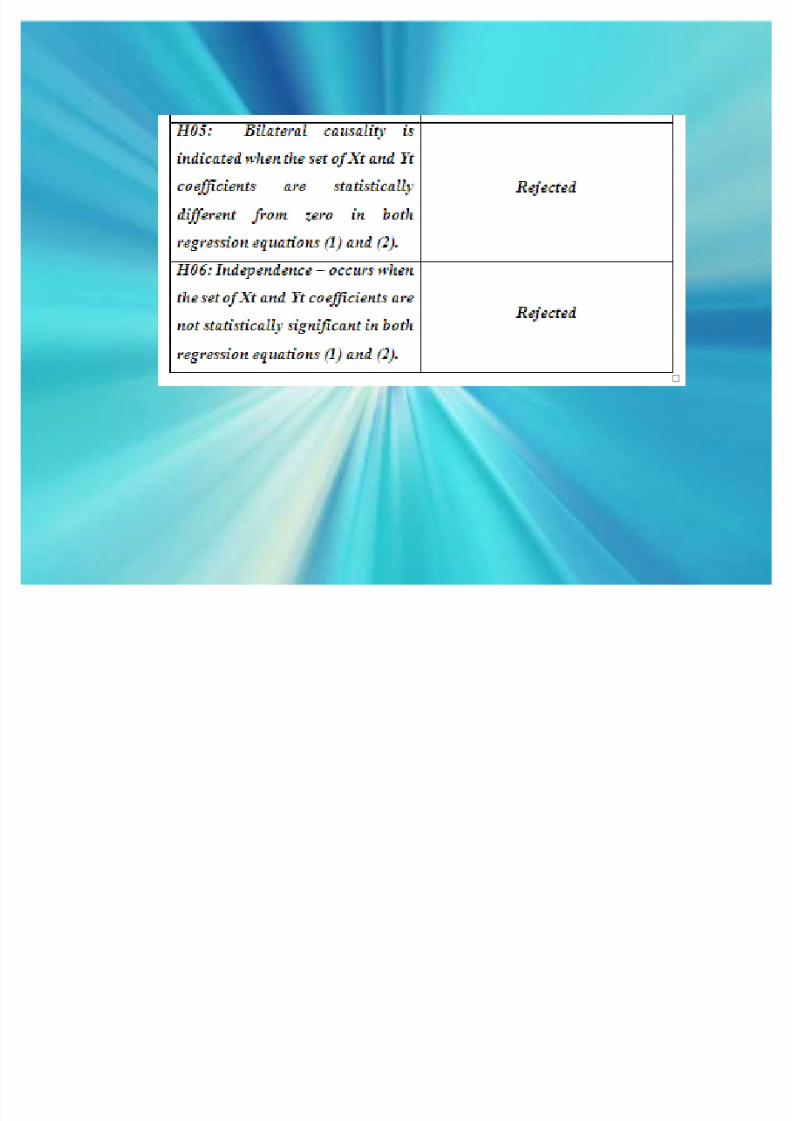
lagged Y t in (2) are statistically different from zero as a group. H0 5: Bilateral causality is indicated when the set of X t and Y t coefficients are statistically

different from zero in both regression equations (1) and (2).

H0 6: Independence occurs when the set of X t and Y t coefficients are not statistically

significant in both regression equations (1) and (2).

In all four cases it is assumed that the two variables Xt andY

t are stationary. In a stochasticprocess stationary means that the statistical characteristics of the process do not change in

time. As Granger and Newbold (1974) and Cheng (1996) point out, Granger causality on non-

stationarity time data may lead to spurious causal relation. The stationarity of a non-stable

time series can be obtained with the help of certain mathematic procedure, such as

differentiation of variables (Gujarati, 2004).



Research Methodology

In the first step of the analysis the stationarity

of the variables was to be examined. If all the

variables are stationary I(0), if there is no

problem to estimate the coefficients using the

variables with initial specification. However,

most of the main macroeconomic variables

are non-stationary, integrated of order higherthan zero.



If the series are non-stationary but co-

integrated, then the estimation as anautocorrected model is admissible. If the

variables are non-stationary and are not co-

integrated then the specification of variables

as differences is necessary.

We used the Augmented Dickey-Fuller test

(ADF) to test the existence of unit roots and to

determine the order of integration of the

variables. The test was conducted with and

without a time trend.



In order to test the co-integration of the

analyzed variables, we used the maximumlikelihood estimation method of Johansen and

Juelius (1990, 1995), since the cointegration

test procedures of Johansen and Juselius

(1990) can distinguish between the existence

of one or more cointegrating vectors and also

generate test statistics with exact distributions

(Van den Berg and Jayanetti 1993); it is herebyappropriate to utilize.



Thus, assuming a vector autoregressive (VAR) model:

xt=ixt-i + xt-1 + + t

Where xt is a vector of non-stationary variables p x 1 and (i =1,.,k). In essence, the JJ (Johansen and Juselius) method

tests whether the coefficient matrix reflects the

fundamentals of long run equilibrium among the non-

stationary variables. As a result, if 0 < rank = r < p, then

there are matrices and of dimension p x r where =

and r cointegrating relations among elements of xt; where

and are cointegration vectors and error correction

parameters, respectively. Both Eigen value and trace tests,

without a trend and with a trend were estimated. Accordingto Sims et all (1990), if the times series are non-stationary and

not co-integrated, then they obtained F statistics used to

detected Granger causality are not valid. Finally we shall apply

the Granger causality to test the hypothesis.



Results

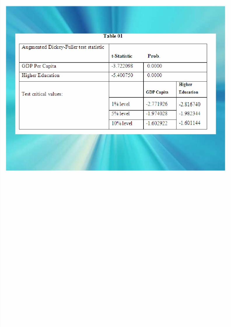
The results of Augmented Dickey-Fuller test

(ADF) to test the existence of unit roots and to

determine the order of integration of the

variables both tests showed that the variables

higher Education and GDP are non-stationary,

at the 5% significance level. However, the non-

stationary problem vanished after seconddifference



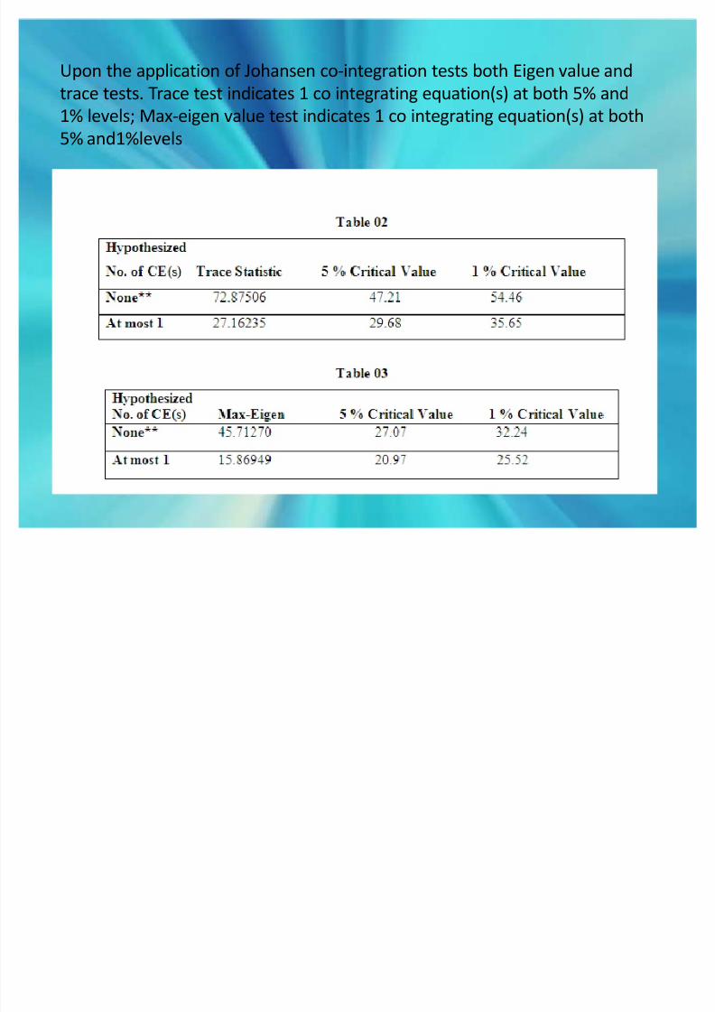
Upon the application of Johansen co-integration tests both Eigen value and

trace tests. Trace test indicates 1 co integrating equation(s) at both 5% and

1% levels; Max-eigen value test indicates 1 co integrating equation(s) at both

5% and1%levels



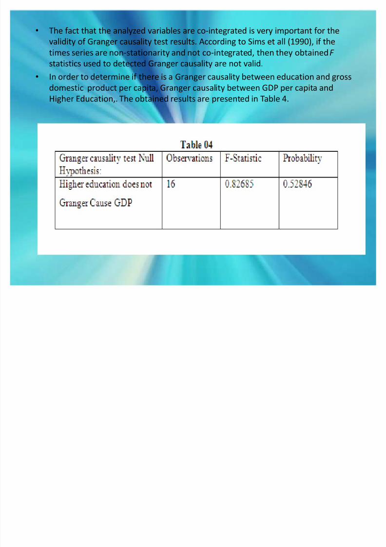
The fact that the analyzed variables are co-integrated is very important for the

validity of Granger causality test results. According to Sims et all (1990), if the

times series are non-stationarity and not co-integrated, then they obtained F

statistics used to detected Granger causality are not valid.

In order to determine if there is a Granger causality between education and gross

domestic product per capita, Granger causality between GDP per capita and

Higher Education,. The obtained results are presented in Table 4.



Conclusion

The aim of this article was to analyze the causality between

education and economic growth for India, in between 1994 -

95 and 2009-10. Using data gathered from IMF website and

from the websites of Index Mundi Using VAR methodology,

we found out that there is empirical evidence of a long-run

relationship between higher-education and gross domestic

product per capita in India, during the analyzed period. , Like

in case of many other BRIC countries like Brazil and China and

very close to the results obtained in Romania by Daniela andLucian (2005) Granger test showed a unidirectional causality

running from gross domestic product per capita to higher

education

international conference ppt

Documents