intermediary asset pricing - booth school of...

American Economic Review 2013, 103(2): 732–770 http://dx.doi.org/10.1257/aer.103.2.732

732

Intermediary Asset Pricing†

By Zhiguo He and Arvind Krishnamurthy*

We model the dynamics of risk premia during crises in asset mar-kets where the marginal investor is a financial intermediary. Intermediaries face an equity capital constraint. Risk premia rise when the constraint binds, reflecting the capital scarcity. The cali-brated model matches the nonlinearity of risk premia during crises and the speed of reversion in risk premia from a crisis back to pre-crisis levels. We evaluate the effect of three government policies: reducing intermediaries borrowing costs, injecting equity capital, and purchasing distressed assets. Injecting equity capital is particu-larly effective because it alleviates the equity capital constraint that drives the model’s crisis. (JEL E44, G12, G21, G23, G24)

The performance of many asset markets—e.g., prices of mortgage-backed securi-ties, corporate bonds, etc.— depend on the financial health of the intermediary sector, broadly defined to include traditional commercial banks as well as investment banks and hedge funds. The 2007–2009 subprime crisis and the 1998 hedge fund crisis are two compelling data points in support of this claim.1 Traditional approaches to asset pricing ignore intermediation, however, by invoking the assumption that intermedi-aries’ actions reflect the preferences of their client-investors. With this assumption, the traditional approach treats intermediaries as a “veil,” and instead posits that a representative household is marginal in pricing all assets. Thus, the pricing kernel for the Standard & Poor’s (S&P) 500 stock index is the same as the pricing kernel for mortgage-backed securities. Yet many crises, such as the subprime crisis and the 1998 episode, play out primarily in the more complex securities that are the province of the intermediary sector. The traditional approach cannot speak to this relationship between financial intermediaries and asset prices. It sheds no light on why “interme-diary capital” is important for asset market equilibrium. It also does not allow for a

1 There is a growing body of empirical evidence documenting the effects of intermediation constraints (such as capital or collateral constraints) on asset prices. These studies include research on mortgage-backed securities (Gabaix, Krishnamurthy, and Vigneron 2007), corporate bonds (Collin-Dufresne, Goldstein, and Martin 2001), default swaps (Berndt et al. 2005), catastrophe insurance (Froot and O’Connell 1999), and index options (Bates 2003; Garleanu, Pedersen, and Poteshman 2009). Adrian, Etula, and Muir (2012) show that an intermediary pricing kernel based on intermediary balance sheet information can explain the cross section of asset returns.

* He: Booth School of Business, University of Chicago, 5807 South Woodlawn Avenue, Chicago, IL 60637, and NBER (e-mail: [email protected]); Krishnamurthy: Kellogg School of Management, Northwestern University, 2001 Sheridan Road, Evanston, IL 60208, and NBER (e-mail: [email protected]). We thank Patrick Bolton, Markus Brunnermeier, Doug Diamond, Andrea Eisfeldt, Vadim Linetsky, Mark Loewenstein, Pablo Kurlat, Tyler Muir, Amir Sufi, Annette Vissing-Jorgensen, Neng Wang, Hongjun Yan, and semi-nar participants at UC-Berkeley, Boston University, the UCSB-LAEF conference, University of Chicago, Columbia University, ESSFM Gerzensee, FDIC, University of Maryland, NBER Asset Pricing, NBER Monetary Economics, NBER EFG, NY Fed, SF Fed, and Yale for their comments. We also thank an anonymous referee for advice.

† To view additional materials, visit the article page at http://dx.doi.org/10.1257/aer.103.2.732.

http://dx.doi.org/10.1257/aer.103.2.732

mailto:[email protected]




733He and KrisHnamurtHy: intermediary asset PricingVOL. 103 nO. 2

meaningful analysis of the policy actions, such as increasing intermediaries’ equity capital or discount window lending, that are commonly considered during crises.

We offer a framework to address these issues. We develop a model in which the intermediary sector is not a veil, and in which its capital plays an important role in determining asset market equilibrium. We calibrate the model to data on the inter-mediation sector and show that the model performs well in replicating asset market behavior during crises.

The striking feature of financial crises is the sudden and dramatic increase of risk premia. For example, in the hedge fund crisis of the fall of 1998, many credit spreads and mortgage-backed security spreads doubled from their precrisis lev-els. Our baseline calibration can replicate this dramatic behavior. When interme-diary capital is low, losses within the intermediary sector have significant effects on risk premia. When capital is high, however, losses have little to no effect on risk premia. The asymmetry in our model captures the nonlinearity that is present in asset market crises. Simulating the model, we find that the average risk pre-mium when intermediaries’ capital constraint is slack is about 3 percent. Using this number to reflect a precrisis normal level, we find that the probability of the risk premium exceeding 6 percent, which is about twice the “normal” level, is 1.33 percent.

Another important feature of financial crises is the pattern of recovery of spreads. In the 1998 crisis, most spreads took about ten months to halve from their crisis-peak levels to precrisis levels. In the subprime crisis, the half-life of most bond market spreads was about six months. As we discuss later in the paper, half-lives for recovery of between six months and extending over a year have been documented in a variety of asset markets and crisis situations. We note that these types of recovery patterns are an order of magnitude slower than the daily mean reversion patterns documented in the market microstructure literature (e.g., Campbell, Grossman, and Wang 1993). A common wisdom among many observers is that this recovery reflects the slow movement of capital into the affected markets (Froot and O’Connell 1999; Berndt et al. 2005; Mitchell, Pedersen, and Pulvino 2007; Duffie and Strulovici 2011). Our baseline calibration of the model can replicate these speeds of capital movement. We show that simulating the model starting from an extreme crisis state (risk premium of 12 percent), the half-life of the risk premium back to the uncon-ditional average risk premium is 8 months. From a risk premium of 10 percent, the half-life is 11 months.

We also use the model as a laboratory to quantitatively evaluate government poli-cies. Beginning from an extreme crisis state with risk premium of 12 percent, we trace the crisis recovery path conditional on three government policies: (i) infus-ing equity capital into the intermediaries during a crisis; (ii) lowering borrowing rates to the intermediary, as with a decrease in the central bank’s discount rate; and, (iii) direct purchase of the risky asset by the government, financed by debt issuance and taxation of households. These three policies are chosen because they are among those undertaken by central banks in practice. In comparing $205 billion of equity infusion to $1.8 trillion of risky asset purchase, we find that the equity infusion is far more effective in reducing the risk premium. This occurs in our model because the friction in the model is an equity capital constraint. Thus, infusing equity capital attacks the problem at its heart. We find that the interest rate policy is also highly

734 THE AMERICAN ECONOMIC REVIEW ApRIl 2013

effective, uniformly increasing the speed of crisis recovery. This policy is effective because the financial intermediary sector carries high leverage and reducing its bor-rowing rates translates to a large subsidy to the intermediary sector.

The contribution of our paper is to work out an equilibrium model of intermedia-tion that is dynamic, parsimonious, and can be calibrated realistically. The paper is related to a large literature in banking studying disintermediation and crises (see Diamond and Dybvig 1983; Holmström and Tirole 1997; Allen and Gale 2005; and Diamond and Rajan 2005). We differ from this literature in that our model is dynamic, while much of this literature is static. The paper is also related to the lit-erature in macroeconomics studying effects of collateral fluctuations on aggregate activity (Kiyotaki and Moore 1997). In much of the macro literature, equilibrium is derived by log-linearizing around the steady state. As a result, there is almost no variation in equilibrium risk premia, which does not allow the models to speak to the behavior of risk premia in crises. We solve a fully stochastic model that better explains how risk premia vary as a function of intermediary capital. In Bernanke and Gertler (1989), credit spreads are linked to the net worth of the entrepreneurial sec-tor. The action in credit spreads is due to default risk and bankruptcy costs, however, rather than due to changes in economic risk premia. Brunnermeier and Sannikov (2011) is another recent paper that develops a macroeconomic model that is fully stochastic and links intermediaries’ financing positions to risk premia. Our paper is also related to the literature on limits to arbitrage studying how impediments to arbitrageurs’ trading strategies may affect equilibrium asset prices (Shleifer and Vishny 1997). One part of this literature explores the effects of margin or debt con-straints for asset prices and liquidity in dynamic models (see Aiyagari and Gertler 1999; Gromb and Vayanos 2002; Fostel and Geanokoplos 2008; Adrian and Shin 2010; and Brunnermeier and Pedersen 2009). Our paper shares many objectives and features of these models. The principal difference is that we study a constraint on raising equity capital, while these papers study a constraint on raising debt financ-ing. Xiong (2001) and Kyle and Xiong (2001) model the effect of arbitrageur capital on asset prices by studying an arbitrageur whose risk aversion varies based on a wealth effect arising from log preferences. The effects that arise in our model are qualitatively similar to these papers. An advantage of our paper is that intermedi-aries and their equity capital are modeled explicitly, allowing our paper to better articulate the role of intermediaries in crises.2 Finally, many of our asset pricing results come from assuming that some markets are segmented and that households can only trade in these markets by accessing intermediaries. Our paper is related to the literature on asset pricing with segmented markets (see Basak and Cuoco 1998; Alvarez, Atkeson, and Kehoe 2002; and Edmond and Weill 2009).3

Our paper is closely related to a companion paper, He and Krishnamurthy (2012). We solve for the optimal intermediation contract in that paper, while we assume the (same) form of contract in the current analysis. That paper also solves for the equilibrium asset prices in closed form, while we rely on numerical solutions

2 The paper is also related to Vayanos (2004), who studies the effect of an open-ending friction on asset-demand by intermediaries. We study a capital constraint rather than an open-ending friction.

3 Our model is also related to the asset pricing literature with heterogenous agents (see Dumas 1989 and Wang 1996).


in the present paper. On the other hand, that paper has a degenerate steady state distribution that does not allow for a meaningful simulation or the other quantita-tive exercises that we perform in the present paper. In addition, the present paper models households with labor income and an intermediation sector that always carries some leverage. Both aspects are important in calibrating the model realisti-cally. Apart from these differences, the analysis in He and Krishnamurthy (2012) provides theoretical underpinnings for some of the assumptions we make in this paper.

The paper is organized as follows. Sections I and II outline the model and its solution. Section III explains how we calibrate the model. Section IV presents the results of the crisis calibration. Section V studies policy actions. Section VI con-cludes followed by a short mathematical Appendix. An online Appendix provides further details of the model solution.

I. The Model: Intermediation and Asset Prices

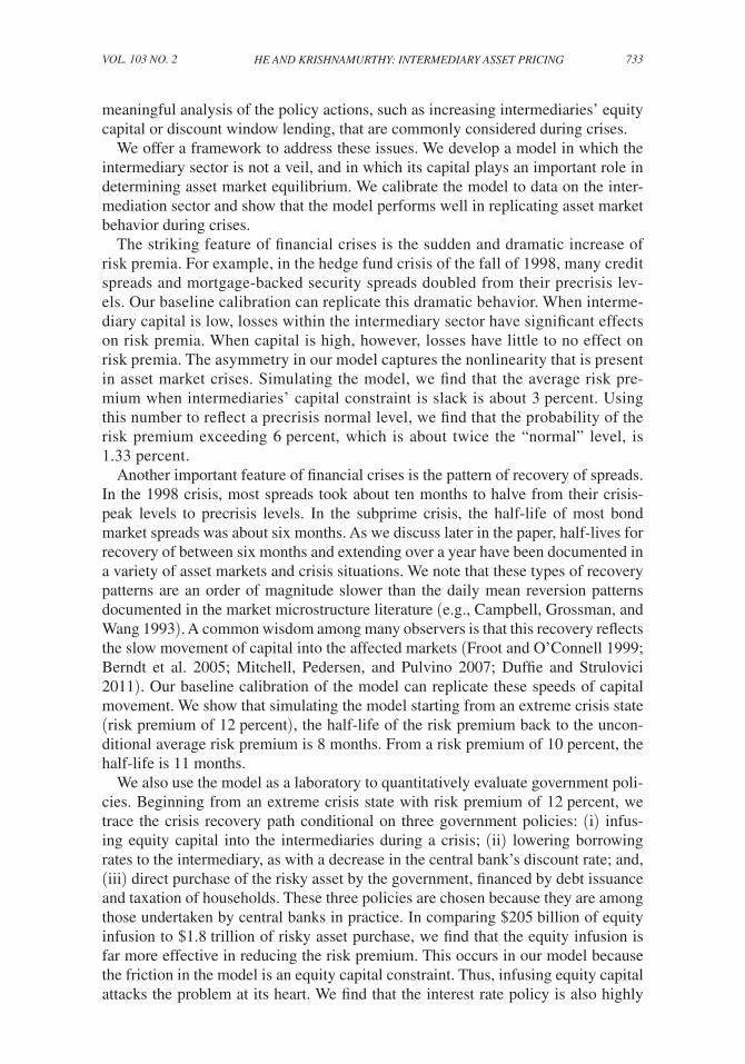
Figure 1 lays out the building blocks of our model. There is a risky asset that represents complex assets where investment requires some sophistication. In our calibration, we match the risky asset to the market for mortgage-backed securities, as a representative large asset class that fits this description.

Investment in the mortgage-backed securities market is dominated by financial institutions rather than households, and sophisticated prepayment modeling is an important part of the investment strategy. The calibration is also appropriate for

Figure 1. Agents in the Economy and Their Investment Opportunities

SPECIALISTS/INTERMEDIARIES

HOUSEHOLDS

RISKY ASSETMARKET

RISKLESSASSETMARKET

HtEQUITY

DEBT


analyzing the financial crisis that began in 2007, where mortgage-backed securities have a prominent role.

There are two groups of agents in the economy, households and specialists. We assume that households cannot invest directly in the risky asset market. There is limited market participation, as in Mankiw and Zeldes (1991); Basak and Cuoco (1998); or Vissing-Jorgensen (2002). Specialists have the knowledge to invest in the risky assets, and unlike in the limited market participation literature, the specialists can invest in the risky asset on behalf of the households. This investment conduit is the intermediary of our model. In our model, the households demand intermediation services while the specialists supply these services. We are centrally interested in describing how this intermediation relationship affects and is affected by the market equilibrium for the “intermediated” risky asset.

We assume that if the household does not invest in the intermediary, it can only invest in a riskless short-term bond. This is clearly counterfactual (i.e., households invest in the S&P 500 index), but simplifies the analysis considerably.

Households thus face a portfolio choice decision of allocating funds between pur-chasing equity in the intermediaries and the riskless bond. The intermediaries accept H t of the household funds and then allocate their total funds under management between the risky asset and the riskless bond. We elaborate on each of the elements of the model in the next sections.

A. Assets

The assets are modeled as in the Lucas (1978) tree economy. The economy is infi-nite-horizon, continuous-time, and has a single perishable consumption good, which we will use as the numeraire. We normalize the total supply of intermediated risky assets to be one unit. The riskless bond is in zero net supply and can be invested in by both households and specialists.

The risky asset pays a dividend of D t per unit time, where { D t } follows a geomet-ric Brownian motion (GBM):

(1) d D t _ D t

= gdt + σd Z t given D 0 ;

g > 0 and σ > 0 are constants. Throughout this paper { Z t } is a standard Brownian motion on a complete probability space ( Ω, , ) . We denote the processes { P t } and { r t } as the risky asset price and interest rate processes, respectively. We also define the total return on the risky asset as

(2) d R t = D t dt + d P t _ P t

.

B. Specialists and Intermediation

There is a unit mass of identical specialists who manage the intermediaries in which the households invest. The specialists represent the insiders/decision-makers


of a bank, hedge fund, or mutual fund. They are infinitely lived and maximize objec-tive function

(3) E [ ∫ 0 ∞ e −ρt u( c t )dt ] ρ > 0,

where c t is the date t consumption rate of the specialist. We consider a constant rela-tive risk aversion (CRRA) instantaneous utility function with parameter γ for the specialists, u( c t ) = 1

_ 1−γ c t 1−γ .

Each specialist manages one intermediary. At every t, each specialist is randomly matched with a household to form an intermediary. These interactions occur instan-taneously and result in a continuum of (identical) bilateral relationships.4 The house-hold allocates some funds H t to purchasing equity issued by the intermediary. We denote the date t wealth of specialists as w t and assume that this is wholly invested in the equity of intermediary. Specialists then execute trades for the intermediary in a Walrasian risky asset and bond market, and the household trades in only the bond market. At t + dt the match is broken, and the intermediation market repeats itself.

Consider one of the intermediary relationships between specialist and household. The specialist manages an intermediary whose total equity capital is the sum of the specialist’s wealth, w t , and the wealth that the household allocates to the intermedi-ary, H t . The specialist makes all investment decisions on this capital and faces no portfolio restrictions in buying or short-selling either the risky asset or the riskless bond. Denote α t I as the ratio of the risky asset holdings of the intermediary to its total capital, w t + H t (this ratio, capturing leverage, will typically be larger than one). Then, the return on capital delivered by the intermediary is

(4) ∼

d R t = r t dt + α t I (d R t − r t dt),

where d R t , defined in equation (2), is the total return on the risky asset. In this nota-tion, α t I > 1 means that the specialist invests more than 100 percent of the interme-diary’s equity capital in the risky assets and thus borrows ( α t I − 1)( w t + H t ) via the riskless short-term bond market, making a leveraged investment in the risky asset.

C. Capital Constraint

The key assumption of our model is that the household is unwilling to invest more than m w t in the equity of the intermediary, where m > 0 is a constant that param-eterizes the financial constraint. If the specialist has one dollar of wealth invested in the equity of the intermediary, the household will only invest up to m dollars of

4 Why the matching structure instead of a Walrasian intermediation market? We study the Walrasian case in He and Krishnamurthy (2012) and find that when intermediation is supply constrained, specialists charge the house-holds a fee for managing the intermediary that depends on the tightness of the intermediation constraint. In par-ticular, the fees rise during financial crises because households see through the intermediaries and determine that economic risk premia are high and as a result compete to give funds to the intermediary to manage. This is clearly counterfactual. We find it unnatural to assume that households who do not participate in the risky asset markets, likely because of informational costs, would be so sophisticated as to be able to compute expected returns as a func-tion of the state. Thus, in the current setting, to keep the model realistic, we adopt the matching structure.


his own wealth in the intermediary. The capital constraint implies that the supply of intermediation facing a household is, at most,

(5) H t ≤ m w t .

If either m is small or w t is small, the household’s ability to participate indirectly in the risky asset market will be restricted with equilibrium effects on risk premia and asset prices.

This type of constraint linking “net worth” and external financing is by now stan-dard fare in the literature on financial frictions (e.g., Holmstrom and Tirole 1997; Kiyotaki and Moore 1997) and can be rationalized by a variety of agency or infor-mational frictions.5 One point worth noting is that the constraint in our model is on the intermediary’s ability to raise outside equity financing rather than outside debt financing. In Kiyotaki and Moore (1997), for example, firms cannot raise any equity financing, while they can raise some debt financing subject to a constraint. An easy way to see that our model describes a constraint on raising equity financ-ing is to observe that both the household and specialist receive the return

∼ d R t (see

equation (4)) on their contributions to the intermediary and hence both hold equity investments in the intermediary. As noted in the introduction, our focus is on an equity capital constraint rather than a debt constraint. Additionally, we place no con-straint on the intermediary’s ability to borrow in the debt market; that is, total debt financing is equal to ( α t I − 1)( w t + H t ) and we place no constraint on this quantity.

When we calibrate the model, we interpret the equity capital requirement in one of two ways. First, the managers of a hedge fund typically have much of their wealth tied up in the hedge fund. Our constraint is that outside investors require that the manager’s stake (“skin in the game”) be sufficient to align incentives. If a hedge fund loses a lot of money, then the stake of the managers of the hedge fund will be depleted. In this case, investors will be reluctant to contribute their own capital to the hedge fund, fearing mismanagement or further losses. A hedge fund “capital shock” is one phenomenon that we can capture with our model. In our calibration, we inter-pret the 20 percent of returns that are typically paid to the hedge fund manager in terms of an incentive contract and the model’s m. Second, the ownership stake inter-pretation also applies more broadly to the banking sector. Holderness, Kroszner, and Sheehan (1999) report that the mean equity ownership of officers and directors in the finance, insurance, and real estate sector was 17.4 percent in 1995. This stake can also be related to the fraction of the intermediary that the specialist owns, w t

_ w t + H t .

The specialist chooses his consumption rate and the portfolio decision of the intermediary to solve

(6) max { c t , α t I }

E [ ∫

0 ∞ e −ρt u( c t ) dt ] s.t. d w t = − c t dt + w t r t dt + w t (

∼ dR t ( α t I ) − r t dt ) ,

5 In a setting that is close to this paper, He and Krishnamurthy (2012) derive this capital constraint by assuming moral hazard by the specialist.


where the intermediary return ∼

dR t ( α t I ) as a function of intermediary portfolio choice α t I is given by equation (4). We can also rewrite the budget constraint in terms of the underlying return:

(7) d w t = − c t dt + w t r t dt + α t I w t ( d R t − r t dt ) .

Note that the intermediary’s portfolio choice of α t I is effectively the specialist’s port-folio share in the risky asset.

D. Households: The Demand for Intermediation

We model the household sector as an overlapping generation (OG) of agents. This keeps the decision problem of the household fairly simple.6 For the sake of clarity in explaining the OG environment in a continuous time model, we index time as t, t + δ, t + 2δ, … and consider the continuous time limit when δ is of order dt. A unit mass of generation t agents are born with wealth w t h and live in periods t and t + δ. They maximize utility:

(8) ρδ ln c t h + ( 1 − ρδ ) E t [ln w t+δ h ];

c t h is the household’s consumption rate in period t and w t+δ h is a bequest for genera-

tion t + δ. Note that both utility and bequest functions are logarithmic.In addition to wealth of w t h , we assume that generation t households receive labor

income at date t of l D t δ. Here, l > 0 is a constant, and recall that D t is the dividend rate on the risky asset at time t. Thus, labor income is proportional to the aggre-gate output of the economy. Introducing labor income for households is important because without such income it is possible to reach states where the household sector vanishes from the economy, rendering our analysis uninteresting (see Dumas 1989 for more on this problem in two-agent models).

A household invests its wealth of w t h from t to t + δ in financial assets. We make assumptions so that the household sector chooses to keep a minimum of λ w t h (λ < 1) in short-term debt issued by the intermediary sector. That is, there is a baseline demand for holding a portion of household wealth in a riskless asset. We think of this in practice as a demand for liquid balances by the household sector that the intermediaries satisfy by issuing bank deposits. This demand is important to our model because it generates leverage in the intermediary sector even in states where the capital constraint does not bind and thus allows us to match leverage ratios of the intermediary sector during noncrisis periods. If we set λ = 0, then the intermediary sector carries no leverage much of the time, which is counterfactual and thus does not allow us to meaningfully calibrate the model.

6 The specialists are infinitely lived while households are modeled using the OG structure. As we will see, spe-cialists play the key role in determining asset prices. Our modeling ensures the choices made by specialists reflect the forward-looking dynamics of the economy. We treat households in a simpler manner for tractability reasons. In He and Krishnamurthy (2012), both specialists and households are long-lived agents. The results are qualitatively similar to the present paper. We adopt the OG structure here because we endow households with labor income. In an incomplete market setting, income from labor complicates the solution to the long-lived household’s problem, considerably.


We model the debt-demand as follows. We assume that a fraction λ of the house-holds can only ever invest in the riskless bond. The remaining fraction, 1 − λ, may enter the intermediation market and save a fraction of their wealth with intermedi-aries that invest indirectly in the risky asset on their behalf. We refer to the former as “debt households” and the latter as “risky asset households.” The wealth of the debt household and risky asset household evolve differently between t and t + δ. We assume that this wealth is pooled together and distributed equally to all agents of generation t + δ. The latter assumption ensures that we do not need to keep track of the distribution of wealth over the households when solving for the equilibrium of the economy.

To summarize, a debt and risky asset household are born at generation t with wealth of w t h . The households receive labor income, choose consumption, and make savings decisions, respecting the restriction on their investment options. It is easy to verify that in the continuous time limit, i.e., when δ → dt, the households’ con-sumption rule is

(9) c t h = ρ w t h .

In particular, note that the labor income does not affect the consumption rule because the labor income flow is of order dt.

The debt household’s savings decision is to invest λ w t h in the bond market at the interest rate r t . The risky asset household with wealth (1 − λ) w t h decides how much to allocate to intermediaries’ equity. Denote α t h ∈ [0, 1] for the fraction of his wealth invested in the intermediaries’ capital and recall that the intermediary’s return is

∼ dR t in equation (4). The remaining 1 − α t h of the risky asset household

wealth is invested in the riskless bond to earn the interest rate of r t dt. Given the log objective function in equation (8), the risky asset household chooses α t h to solve (where we have taken the limit as δ → dt)

(10) max α t h ∈[0, 1]

α t h E t [

∼ dR t − r t dt ] − 1 _

2 ( α t h ) 2 Va r t [

∼ dR t − r t dt ] s.t. α t h (1 − λ) w t h ≡ H t ≤ m w t .

The constraint here corresponds to the intermediation constraint (5) that we have discussed earlier.

Given the decisions by the debt household and the risky asset household, the evo-lution of w t h across generations is described by

(11) d w t h = (l D t − ρ w t h )dt + w t h r t dt + α t h (1 − λ ) w t h ( ∼

dR t − r t dt ) .

E. Equilibrium

DEFINITION 1: An equilibrium is a set of price processes { P t } and { r t }, and deci-sions { c t , c t h , α t I , α t h } such that

(i) Given the price processes, decisions solve the consumption-savings problems of the debt household, the risky asset household (equation (10)) and the spe-cialist (equation (6));


(ii) Decisions satisfy the intermediation constraint of (5);

(iii) The risky asset market clears

(12) α t I ( w t + α t h (1 − λ ) w t h ) __ P t

= 1;

(iv) The goods market clears:

(13) c t + c t h = D t (1 + l).

Given market clearing in risky asset and goods markets, the bond market clears by Walras’ law. The market clearing condition for the risky asset market reflects that the intermediary is the only direct holder of risky assets and has total (equity) funds under management of w t + α t h (1 − λ ) w t h , and the total holding of risky asset by the intermediary must equal the supply of risky assets.

Finally, an equilibrium relation that proves useful when deriving the solution is that

w t + w t h = P t .

That is, since bonds are in zero net supply, the wealth of specialists and households must sum to the value of the risky asset.

II. Solution

We outline the main steps in deriving the solution in this section, highlighting the economic mechanism linking intermediary equity capital and risk premia for the special case of log utility. Detailed derivations are in the Appendix.

A. Equilibrium Risk Premium

We look for a stationary Markov equilibrium where the state variables are ( x t , D t ), where x t ≡ w t

_ P t ∈ ( 0, 1 ) is the fraction of wealth in the economy owned by the spe-

cialists. We refer to the fraction x t as specialist capital. As standard in any economy with CRRA agents where endowments follow a Geometric Brownian Motion as in equation (1). We conjecture that the equilibrium risky asset price is

(14) P t = D t p( x t ),

where p ( x ) is the price/dividend ratio of the risky asset.While the household faces investment restrictions on his portfolio choices, the

specialist (intermediary) is unconstrained in his portfolio choices. This important observation implies that the specialist is always the marginal investor in determining


asset prices, while the household may not be. Standard arguments then tell us that we can express the pricing kernel in terms of the specialist’s equilibrium consumption process. Optimality for the specialist gives us the standard consumption-based asset pricing relations (Euler equation):7

(15) −ρdt − γ E t [ d c t _ c t ] + 1 _ 2 γ (γ + 1)Va r t [ d c t _ c t ] + E t [ d R t ] = γ Co v t [ d c t _ c t , d R t ] ;

and for the interest rate, we have

(16) r t dt = ρdt + γ E t [ d c t _ c t ] − γ(γ + 1)

_ 2 Va r t [ d c t _ c t ] .

Combining these equations gives an expression for the risk premium:

E t [d R t ] − r t dt = γ Co v t [ d c t _ c t , d R t ] .The risk premium depends on the covariance of the asset return with the specialist’s consumption growth.

B. Log-Utility Special Case

Consider the special case where γ = 1 as this case offers a clear characterization of the solution. With log utility, the consumption-to-wealth ratio is constant, imply-ing that consumption growth is equal to wealth growth:

(17) E t [d R t ] − r t dt = Co v t [ d w t _ w t , d R t ] .The specialist’s wealth growth is given in equation (7). The key term driving the return volatility of specialist wealth d w t / w t is the specialist’s leveraged exposure to the risky asset, α t I d R t . Combined with equation (17), this observation implies that

E t [d R t ] − r t dt = α t I Va r t [d R t ].

There are two terms affecting the risk premium: α t I is the intermediary’s exposure to the risky asset, while Va r t [d R t ] is the variance of returns. In our calibration, most

7 The Euler equation is a necessary condition for optimality. In the online Appendix, we prove sufficiency.


of the action in the risk premium is driven by the exposure term rather than the vari-ance. Therefore we consider the exposure term α t I in further detail.

Suppose that the equity capital constraint binds and the intermediaries raise total equity capital of w t + m w t . We refer to this case as being in the constrained region. Since all risky assets are held through the intermediary, the equilibrium market clearing condition (12) in the constrained region gives

α t I, const ( w t + m w t ) = P t .

Rewriting, we find that

(18) α t I, const = 1 _ x t 1 _

1 + m .

Thus, as specialist capital, x t , falls in the constrained region, the risk premium rises. Moreover, when m is larger so that the specialist is able to raise more equity capital from the household for a given amount of his own equity stake, the risk premium effect is dampened.

Next consider the unconstrained region. Total capital of the intermediary sector is equal to the specialist’s capital plus the risky asset household’s capital contribution to the intermediary sector. This gives the market clearing condition for the risky asset,

α t I, unconst ( w t + ( 1 − λ ) w t h α t h ) = P t .

We make an assumption that implies that α t h = 1.

PARAMETER ASSUMPTION 1: We focus on parameters of the model such that in the absence of any portfolio restrictions, the risky asset household will choose to have 100 percent of his wealth invested in the intermediary; i.e., α t h = 1.

Although we are unable to provide a precise mathematical statement for this parameter restriction, in our calibration it appears that the relative risk aversion parameter γ ≥ 1 is a sufficient condition.8 We then have that

(19) α t I, unconst = 1 __ x t + ( 1 − λ ) (1 − x t )

= 1 __ 1 − λ ( 1 − x t )

.

In the case where λ = 0 (no debt households in the economy), α t I, unconst is constant and equal to one. This result implies that the risk premium in the unconstrained region is constant. In contrast, as shown above, the risk premium rises in the constrained region when the intermediary capital falls. This pattern is the central economic fea-ture of our model. There is an asymmetry whereby when the equity capital constraint binds, further reductions in specialist capital cause a large increase in risk premia.

8 Loosely speaking, if the specialist is weakly more risk averse than the household, the household will hold more risky assets than the specialist. But given market clearing in the risky asset market, the specialist always holds more than 100 percent of his wealth in the risky asset. Recall that we assume that the household cannot short bonds. Thus, the equity household allocates the maximum of 100 percent of his wealth to the intermediary.


For the case where λ > 0, which we consider in the calibration, the risk premium also rises in the unconstrained region because of a leverage effect. In our calibration, however, the latter effect is small compared to the effect in the constrained region. Analytically, we can see that the effect of falling x t in the constrained region is more significant than that of falling x t in the unconstrained region by looking at the ratio

(20) α t I, const

_ α t I, unconst

= 1 _ 1 + m

( 1 + ( 1 − λ ) 1 − x t _ x t ) .

The variable α t I, unconst describes the portfolio share as a function of x t if the model

had no capital constraint. Thus, the ratio, α t I, const _

α t I, unconst , describes how much higher α t I

is relative to this benchmark. The key term is 1 − x t _ x t , which is the ratio of house-

hold wealth to specialist wealth. As specialist wealth falls relative to household wealth, 1 − x t

_ x t rises and we see that the equity capital constraint causes the ratio (and hence the risk premium) to rise.

The model also has an amplification effect in the constrained region. Since α t I, const is high in the constrained region, the specialist has a large exposure to the risky asset. Then, a negative dividend shock translates to a large fall in x t , which further increases the risk premium and lowers asset prices.

C. γ > 1 Case

For the general case where γ > 1, specialist consumption is not proportional to wealth and the simple characterization is no longer exact. We solve the model in a different manner in the general case. The market clearing condition for goods (from equation (13)) is

c t + c t h = D t (1 + l).

Since the household with log utility sets consumption c t h = ρ w t h = ρ(1 − x t ) P t , in equilibrium, the specialist consumes

(21) c t = D t (1 + l ) − ρ (1 − x t ) P t = D t [ (1 + l ) − ρ (1 − x t ) p ( x t ) ] .

Using equations (21) and (14), we can express d R t and d c t _ c t in terms of the price/divi-

dend ratio p(x ) and its derivatives. We also need the drift and diffusion of x t . To find these terms, note that x t = w t

_ P t , and the specialist’s wealth w t evolves according to

(22) d w t = − c t dt + w t r t dt + α t I w t ( d R t − r t dt ) .

The key term driving the wealth evolution of the specialist is his portfolio exposure to the risky asset; i.e., α t I . Recall that in the previous section, we derive α t I for the constrained and the unconstrained regions as equations (18) and (19). The deriva-tion is based on market clearing conditions and does not depend on the value of γ. Combining all of these results, we arrive at an ordinary differential equation that must be satisfied by p(x ) (see the mathematical Appendix).


The differential equation is solved for the constrained and unconstrained regions.

The intermediation constraint binds at the point where α t I, const _

α t I, unconst = 1 for equation (20).

Solving, we find that the critical value of x c at which the constraint binds is

(23) 1 _ x c

= 1 + m _ 1 − λ

⇔ x c = 1 − λ _ 1 − λ + m

.

When x < x c , the intermediation constraint binds, while if x > x c the constraint does not bind. If m is high, then x c is low, and hence the constraint binds for less of the state space. If the debt households fraction λ is high, there are less risky asset households looking to invest in the equity of the intermediation sector, and as a result the capital constraint binds for less of the state space.

D. Boundary Condition

In equilibrium, the fraction of specialist capital x t moves in the range ( 0, 1 ) . When x t → 1, the economy behaves as if comprised of specialists only. We derive an expression for the boundary condition for p ( 1 ) in the mathematical Appendix. On the other hand, as x t approaches zero, the economy is comprised mostly of house-holds. The boundary condition in this case is as follows. Consider the specialist’s consumption in equation (21). We must have that specialist consumption approaches zero as x t approaches zero.9 Thus, using equation (14), we have

(24) D (1 + l ) = ρP (x = 0, D) ⇒ p (0) = 1 + l _ ρ .

9 In the argument for verification of optimality of the specialist’s equilibrium strategy that is detailed in the online Appendix, we see that this condition translates to the transversality condition for the specialist’s budget equation. Therefore the boundary condition (24) is sufficient for the equilibrium presented in this paper to be well-defined.

Table 1—Intermediation Data

Group Assets Debt Debt/assets

Commercial banks 11,800 10,401 0.88S&L and credit unions 2,574 2,337 0.91Property and casualty insurance 1,381 832 0.60Life insurance 4,950 4,662 0.94Private pensions 6,391 0 0.00State and local ret funds 3,216 0 0.00Federal ret funds 1,197 0 0.00Mutual funds (excluding money funds) 7,829 0 0.00Broker/dealers 2,519 2,418 0.96Hedge funds 6,913 4,937 0.71

Notes: Most data are from the Flow of Funds March 2010 Level Tables, corresponding to the year 2007, and are reported in billions. The broker/dealer and hedge fund total assets are as computed in He, Khang, and Krishnamurthy (2010), who use data from SEC filings for the broker/dealer sector and data from Barclay’s Hedge for the hedge fund sector. We assume that the average broker/dealer runs a leverage of 25, based on Adrian and Shin (2010). We assume the average hedge fund leverages up its capital base 3.5 times (taken from McGuire, Remolona, and Tsatsaronis 2005).


In the online Appendix, we show that x = 0 is an entrance-no-exit boundary and that x t never reaches x = 0.

III. Calibration

Table 1 provides data on the main intermediaries in the US economy. Households hold wealth through a variety of intermediaries including banks, retirement funds, mutual funds, and hedge funds.

A. Choice of m

The m of the model parameterizes the equity capital constraint of the intermediar-ies. We set m equal to 4, which matches both ownership data of banks and compen-sation data from hedge funds. Holderness, Kroszner, and Sheehan (1999) report that the mean equity ownership of officers and directors in the finance, insurance, and real estate sector was 17.4 percent in 1995. This translates to an m of 4.7(= 1 − 0.174

_ 0.174 ). Hedge fund contracts typically pay the manager 20 percent of the fund’s return in excess of a benchmark, plus 1–2 percent of funds under management (Fung and Hsieh 2006). The choice of m dictates how much of the return of the intermediary goes to the specialist ( 1

_ 1+m ) and how much goes to equity investors ( m

_ 1 + m ) . A value of m = 4 implies that the specialist’s share 1 _

5 = 20 percent. The 20 percent that is

common in hedge fund contracts is an option contract so it is not a full equity stake as in our model, suggesting that perhaps we should use a larger value of m. To bal-ance this, however, note that the 1–2 percent fee is on funds under management and therefore grows as the fund is successful and garners more inflows. We thus settle on a value of m = 4 as representative, in a linear scheme, of the payoff structure of the hedge fund.10

B. Choice of λ

The choice of m only plays a role in driving the intermediary sector’s capital struc-ture when the equity capital constraint binds. In particular, if we set λ = 0, then the leverage of the intermediary sector will be zero when the equity capital constraint does not bind. This is counterfactual as banks always carry debt, even during boom periods when capital constraints are likely slack. Across all of the intermediaries of

10 The m in our calibration applies to the entire intermediation sector, and as is evident in Table 1, there is func-tional heterogeneity across the modes of intermediation. In particular, it is not obvious what the m for the mutual fund or pension fund sector should be, which may lead one to worry about our choice of m based solely on consider-ing the leveraged sector. Our justification for m is as follows. When the intermediation constraint (5) binds, losses among intermediaries lead households to reduce their equity exposure to these intermediaries. If the intermediaries scale down their asset holdings proportionately, the asset market will not clear—i.e., the intermediary sector’s assets still have to be held in equilibrium. In the model, the equilibrium is one where the (identical) intermediaries take on debt and hold a riskier position in the asset. Asset prices are then set by the increased risk/leverage considerations of the intermediaries. In practice, if households withdraw money from mutual funds, then mutual funds do not take on debt. Rather, they reduce their holdings of financial assets and some other entity buys their financial assets. In prac-tice, the other entity will be a trading desk at a bank or a hedge fund that temporarily provides liquidity to the mutual fund rather than a nonleveraged investor. Thus, we see that to model asset price behavior we want m to correspond to the equity capital constraints of banks/hedge funds rather than features of the broad intermediary sector. This is because it is the marginal pricing condition of these intermediaries that is most relevant during a liquidation crisis.


Table 1, the total debt/total assets ratio in 2007 is 0.52. We assume that this was a period when the equity capital constraint was slack and choose λ to target the 0.52 number. We set λ = 0.6, which produces an unconditional average debt-to-asset ratio of 0.55, and a ratio of 0.50 in the unconstrained region.

C. σ and g

We calibrate the intermediated asset to the market for mortgage-backed securities (MBS) as a representative large intermediated asset class. The Securities Industry and Financial Markets Association (SIFMA) reports that the total outstanding MBS securities (agency-backed MBS, private-label MBS, commercial MBS) totaled $8.9 trillion in 2007. SIFMA reports that the outstanding amount of asset-backed securities (auto, credit card, etc.) totaled $2.5 trillion in 2007. We are unaware of data that allow us to know precisely who holds these securities. The pattern of losses as reported by financial institutions in the subprime crisis, however, and most analyses of losses (e.g., the International Monetary Fund’s Global Financial Stability Report of October 2008) suggests these securities are mostly held in intermediary portfolios.

The Barclays Capital US MBS Index (formerly the Lehman Brothers US MBS Index) tracks the return on the universe of agency-backed MBS from 1976 onward. The annual standard deviation of the excess return of this index over the Treasury bill rate, using data from 1976 to 2008, is 8.1 percent. Note that this index measures the returns on agency-backed MBS, which is the least risky (although largest) seg-ment of the MBS market. As another benchmark, the annual standard deviation of the excess return on Barclays Index of commercial MBS over the period 1999 (i.e., inception of the index) to 2008 is 9.6 percent.

We choose σ to be 9 percent. With this choice, the standard deviation of the excess return on the intermediated asset in our model is 9.2 percent. This number is in the range between the low-risk agency MBS and the higher-risk commercial MBS.

We choose g = 2 percent to reflect average per capita growth in US GDP. We would expect that the payouts on mortgage assets should grow with the economy. The choice of g has a minor effect on results. On the other hand, σ is critical because it is closely related to the amount of risk borne by the specialist and the volatility of the intermediary pricing kernel.

D. γ, l, and ρ

We choose γ = 2 as risk aversion of the specialist. This choice of γ produces an average excess return on the intermediated asset of 3.36 percent. Over the 1976 to 2008 period, the average excess return on the Barclay’s Agency MBS Index was 2.6 percent. Over the 1999 to 2008 period, the return on the commercial MBS index was 0.32 percent. The latter sample is quite short, however, and heavily weighted by a large −22.9 percent return in 2008.

We choose l based on the share of labor income to total income for the United States, which is 66 percent from aggregate income statistics. In the model, house-holds receive labor income of l D t . We also classify the capital gains and dividend income that specialists receive from running intermediaries as labor income. That is, for a hedge fund, the labor income of the manager comes from his 20 percent stake


in the returns of the fund. We set l = 1.84, which produces an average household-plus-specialist labor to total income in the model of 64.5 percent.

We choose ρ = 0.04. This choice produces an average riskless interest rate of 0.06 percent, which is lower than the typical numbers in the literature (0.5 percent). Our parameter choices are also dictated by the restriction that

ρ + g(γ − 1) − γ (γ−1) σ 2 _ 2 − l γ ρ

_ 1 + l > 0. This restriction is necessary to ensure that

the economy is well-behaved at x = 1 (see the mathematical Appendix). Given our other parameter choices, setting ρ higher violates this condition.

IV. Results

This section presents results from solving the model, beginning by showing how risk premia are related to specialist capital, and then showing measures from simulating the model. The mathematical Appendix describes details on the solution and simulation method.

A. Risk Premium as a Function of Specialist Capital

Figure 2 graphs the risk premium for the calibration of Table 2 as a function of x, the specialist capital relative to the value of the risky asset (w/P). The prominent feature of our model, clearly illustrated by the graphs, is the asymmetric behavior of the risk premium. The right-hand side of the graph represents the unconstrained states of the economy, while the left-hand side represents the constrained states. The cutoff for the constrained region in the figures is x c = 1−λ _

1−λ+m = 0.091. In words,

the constrained region arises when specialists own no more than equity equivalent to 9.1 percent of the assets held by intermediaries. Note that this number refers to the equity ownership of the entire intermediation sector; there may be some sectors where the specialists own far less than 9.1 percent, and some where the specialists own more. Risk premia rise as specialist wealth falls in the constrained region, while being relatively constant in the unconstrained region.

Figure 2. Risk Premium

Notes: Risk premium and intermediary’s portfolio share in the risky asset are graphed against x = w/P, the special-ist’s wealth as a percentage of the assets held by the intermediation sector. Parameters are those given in Table 2.

0 0.05 0.1 0.15 0.2 0.25 0.302468

101214161820

w/P

Intermediary’s Position in Risky Asset (αI

Constrainedregion

Unconstrained region

)

0 0.05 0.1 0.15 0.2 0.25 0.30

0.020.040.060.08

0.10.120.140.160.180.2

w/P

Risk Premium

Constrainedregion

Unconstrained region


As discussed in Section IIB, the asymmetry in the risk premium is driven by the rising portfolio share α t I . The right panel of the figure graphs this portfolio share as a function of specialist capital. Note the close relation between this figure and that for the risk premium. Finally, note that the effect in the constrained region is nonlinear. If capital halves from x = 0.091 to x = 0.045, the risk premium only rises modestly from about 4 percent to 5 percent. The risk premium rises much more as capital falls below x = 0.045.

An interesting point of comparison for our results is to the literature on state-dependent risk premia, notably, Campbell and Cochrane (1999); Barberis, Huang, and Santos (2001); and Kyle and Xiong (2001). In these models, as in ours, the risk premium is increasing in the adversity of the state. Campbell and Cochrane (1999) and Barberis, Huang, and Santos (2001) modify the utility function of a representative investor to exhibit state-dependent risk aversion. We work with a standard CRRA utility function, but generate state dependence endogenously as a function of the frictions in the economy. In this regard, our model is closer in spirit to Kyle and Xiong (2001), who generate a risk premium that is a function of “arbitrageur” wealth. The main theoretical difference between Kyle and Xiong and our model is that the wealth effect in their model comes from assuming that the arbitrageur has log utility, while in our model it comes because the intermediation constraint is a function of intermediary capital. For empirical work, our model sug-gests that measures of intermediary capital will explain risk premia. One notable distinction of our model is the sharp asymmetry of our model’s risk premia: a muted dependence on capital in the unconstrained region and a strong dependence in the constrained region. In Kyle and Xiong (2001), the log utility assumption delivers a risk premium that is a much smoother function of arbitrageur wealth. Plausibly, to explain a crisis episode, one needs the type of asymmetry delivered by the con-straints we model.

B. Discussion: Leverage and Heterogeneity

Figure 2 indicates that the rise in the risk premium in the constrained region is closely related to the rise in leverage of the intermediary sector. The ratio of total intermediary sector assets to intermediary equity, or accounting leverage, is equal to α I . Thus, our model implies that the leverage of the intermediary sector rises during a crisis.

In practice, many intermediary sectors during a crisis reduce leverage, while other sectors increase leverage. There is heterogeneity within the intermediation sector that our single intermediary model cannot capture. Adrian and Shin (2010) docu-ment that the leverage of the broker/dealer sector is procyclical, suggesting that it falls during recessions and crises. The Adrian and Shin evidence, however, is based on data from the Federal Reserve’s flow of funds, which is measured in terms of book values. The α I of our model corresponds to market value leverage.11

11 The average amount of credit extended by households to intermediaries in the constrained region, measured as ( λ w h + ( 1 − λ ) ( 1 − α h ) w h ) /D, is 83 percent of the amount of credit extended by households in the uncon-strained region. That is, as a fraction of GDP our model predicts that the household sector extends less credit to the intermediary sector during crises. The market value of intermediary equity falls more than this reduction in debt borrowing, however, which therefore drives up market value leverage in the model. If we instead held market value


Ang, Gorovyy, and van Inwegen (2011) show that if one uses market value of equity in computations, then leverage of the broker/dealer sector rises during the 2008 crisis. They also document that the leverage of the hedge fund sector falls dur-ing the crisis. He, Khang, and Krishnamurthy (2010) document that in the period from the fourth quarter of 2007 to the first quarter of 2009, spanning the worst episode of the subprime crisis, the hedge fund sector sheds assets, consistent with Adrian and Shin (2010). He, Khang, and Krishnamurthy (2010) also show that the commercial banking sector increased asset holdings over this period significantly. Moreover, the leverage of the top 19 commercial banks sector rises from 10.4 at the end of 2007 to near 30 at the start of 2009. The differential behavior of the banking sector in 2008 is reflective of a broader pattern of reintermediation during financial downturns, as documented by Gatev and Strahan (2006) and Pennacchi (2006). Importantly for the present analysis, in accord with our model the intermediaries that are the buyers during the crisis (i.e., banks) do so by borrowing and increasing leverage. Our model does not capture the other aspect of this process, as reflected in the behavior of the hedge fund sector, that some parts of the financial sector reduce asset holdings and deleverage.

C. Steady State Risk Premia

Quantitatively, as one can read from Figure 2, the calibration produces a risk pre-mium in the unconstrained region of approximately 3 percent.12 The numbers for the risk premium are higher in the constrained region. To provide some sense for the

of equity fixed—loosely corresponding to an accounting book measure that responds slowly to market prices—then our model implies that book leverage falls in a crisis. In this way, our model can be made consistent with the Adrian and Shin (2010) evidence.

12 More precisely, the average risk premium conditional on being in the unconstrained region is 3.07 percent.

Figure 3. Steady State Distribution

Notes: The steady state distribution of x = w/P is graphed. Left panel is for the baseline parameters, while right panel is for γ = 1. The vertical line at x c = 1−λ _

1−λ+m gives the state where the intermediation constraint starts binding.

The dashed line graphs the risk premium in order to illustrate the actual range of variation of the risk premium. Risk premium is indicated on the left scale, while the distribution is indicated on the right scale.

w/P

0 0.1 0.2 0.3 0.4 0.5 0.6 0.7 0.8

0

0.1

0.2

0.3

0.4

0.5

0.6

0.7

0.8

0.9

0 0.1 0.2 0.3 0.4 0.5 0.6 0.7 0.80

0.05

0.1

0.15

w/P0 0.1 0.2 0.3 0.4 0.5 0.6 0.7 0.8

0

0.05

0.1

0.150 0.1 0.2 0.3 0.4 0.5 0.6 0.7 0.8

0

0.1

0.2

0.3

0.4

0.5

0.6

0.7

0.8

0.9


values of the risk premium we may be likely to observe in practice, we simulate the model and compute the equilibrium probability of each state. The resulting steady state distribution over x is graphed in Figure 3. Also superimposed on the figure in a dashed line is the risk premium from the previous graph.

There are two forces driving the center-peaked distribution in Figure 3. First, as x falls, the risk premium rises. This in turn means that the specialist’s wealth, due to the levered position in the risky asset, is expected to increase as time passes, which tends to push x back to the original level. This force is stronger as the risk premium rises, which is why the distribution places almost no weight on risk premia as high as 30 percent. At the other end, when x is large so that w h is small, the households are poor and consume little but still receive labor income. Thus, their wealth grows as they save the labor income, which shifts the wealth distribution back toward the center of the distribution.

The left panel of the figure is for the baseline parameters, while the right panel is for the γ = 1 case. For this latter case, the entire steady-state distribution is shifted

Table 3—Measurements

Baseline σ = 6 γ = 1 m = 8 λ = 0.05 l = 1

Risk premium (%) 3.36 1.96 2.35 3.38 3.25 3.19Sharpe Ratio (%) 36.46 32.62 27.34 37.11 35.72 34.81Return volatility (%) 9.25 6.12 10.60 9.17 9.23 9.18Interest rate (%) 0.06 1.42 0.95 0.02 0.14 0.83Labor income ratio 0.64 0.52 0.54 0.62 0.55 0.61Price/dividend 70.50 70.02 71.00 71.00 70.22 49.50Prob(unconstrained)(%) 65.50 12.48 39.40 78.95 0.91 78.35Debt/assets ratio 0.50 0.49 0.52 0.52 0.00 0.48 (unconstrained)Prob(RiskPremium > 0.87 1.99 3.49 0.55 1.43 0.57 2 ×

__________ RiskPremium )

E(RiskPremium | > 8.89 5.23 7.41 9.40 8.60 8.41 2 ×

__________ RiskPremium )

Notes: We present a number of key moments from the model. We report the unconditional average risk premium, Sharpe ratio, volatility, interest rate, and labor-to-total income ratio. We also report the unconditional probability of the capital constraint not binding, and the Debt/assets ratio of the intermediary sector conditional on the capital constraint not binding. The last two rows provide information on the tails of the distribution, where the risk pre-mium is at least double its unconditional average. In the first column, we report measure for the baseline param-eterization. The rest of the columns consider variations where we change a single parameter relative to the baseline given in Table 2.

Table 2—Parameters and Targets

Panel A. Intermediation

m Intermediation multiplier 4 Compensation of financial managersλ Debt ratio 0.6 Debt/assets of intermediary sector

Panel B. Preferences and cashflows

g Dividend growth 2% Growth of economyσ Dividend volatility 9% Volatility of MBS portfolioρ Time discount rate 4% Short-term interest rateγ Relative risk aversion of specialist 2 Risk premium on MBS portfoliol Labor income ratio 1.84 Share of labor income in total

income


to the left. As we explain in the next section, this result is due to greater risk-taking by the intermediary sector.

D. Measurements from Simulation

The first column of Table 3 corresponds to the baseline parameterization of Table 2. Parameters have been chosen to match the risk premium, return volatility, interest rate, labor-to-total income ratio for the economy, and the debt/assets ratio of the intermedi-ary sector when the capital constraint does not bind. As a result, the fit of the model in these dimensions is as expected. On the other hand, none of the parameters are explic-itly chosen to match patterns during crises. The last two rows focus on tails of the simulated distribution when the risk premium exceeds twice its unconditional average. In the next sections, we will further explore the behavior of the model in this tail.

Before doing so, we focus in this section on explaining how the model’s param-eters affect the results, which are presented in columns 2 through 6 in Table 3, where we change a single parameter relative to the baseline.

Risk prices: γ and σ.—The first two variations consider changes in the risk aver-sion γ of the specialist and the fundamental risk of the economy σ.

As expected, relative to the baseline of γ = 2, setting γ = 1 decreases the risk premium and Sharpe ratio. It also increases interest rates because of the dampening of the precautionary savings effect. The interesting result is a “risk-taking” effect. With lower risk-aversion, the intermediary sector is willing to hold a more risky portfolio. Hence, the same fundamental volatility is translated to a greater volatility for the specialist’s wealth, and the economy is more likely to enter the constrained region. The effect is reinforced through a general equilibrium effect. While the total risk in our economy is relatively stable due to the endowment structure, when the specialist has lower risk aversion, the price of risk falls and causes the intermediary to be compensated less per unit of risk.13 Hence, the intermediary sector on aver-age earns and retains fewer profits, which in turn leads the capital constraint to bind more frequently.

In Table 3, this “risk-taking” effect is reflected in a smaller Prob(unconstrained) of 39.4 percent (relative to 65.5 percent in the baseline). We can also see this effect in the tails of the distribution, which are in the last two rows of Table 3. There, the probability of hitting the double-average-risk-premium states rises. Graphically, this effect is apparent from Figure 3, where we see that the γ = 1 case causes the entire distribution to shift toward crisis-states.

The above general equilibrium effect also plays a role in the results for a lower fundamental volatility σ = 6 percent. Not surprisingly, reducing σ decreases the risk premium, Sharpe ratio, and return volatility. The surprising result in this case is that the probability of the unconstrained region decreases. That is, a lower cash flow volatility leads to the capital constraint binding more frequently. This result is due to the lower average risk premium demanded by the economy with relatively low fundamental risk, which again lowers average intermediary sector profits.

13 Although when γ = 1, we find that the return volatility rises relative to the baseline γ = 2, which leads to a small compounding effect beyond the direct effect of a lower price of risk.


Intermediation: m and σ.—The next two variations focus on changing the inter-mediation parameters. The case with m = 8 shows that most of the unconditional asset market measures do not depend on m. The main effect is on the probability of hitting the constraint. With a higher m, the capital constraint is loosened, and hence the probability of hitting the constraint falls. The probability of doubling the risk premium also falls. But note that with m = 8, the average risk premium in these states rises. This latter effect is due to a “sensitivity” effect of m. With a higher m, a one dollar fall in specialist capital leads to larger withdrawal of household capital, which increases the sensitivity of the risk premium to the specialist capital.14

The next column considers the effect of setting λ near zero. This variation has the expected effect of lowering the debt/assets ratio in the unconstrained region to near zero. Like the variation with m, changing λ has little effect on the unconditional asset market measures. The main effect again is on the probability of hitting the constraint. From equation (23) we see that lowering λ increases x c .15 Effectively, the entire steady-state distribution shifts toward constrained regions, with the λ = 0.05 case presented in the table giving an unconstrained probability of near zero. We opt in our baseline for a higher λ primarily because doing so implies that the equity capital constraint only binds occasionally.

Labor Income l.—The last case in the table demonstrates the effect of lowering l. With a lower l, the probability of being in the constrained region falls. Intuitively, because households have less income per period, the specialist wealth tends to grow faster relative to the household wealth, and as a result the economy spends more time away from the capital-constrained region. We also see this effect in the last lines of the table. The probability of hitting the high-risk premium states falls when l falls. These effects in turn lower the average risk premium. The most significant effect of l is on the average price/dividend ratio. With lower labor income, households save less money every period, which lowers their demand for assets, leading to lower asset prices. This effect is most evident from the boundary condition, equation (24); there, we see that asset values are scaled down commensurately with a lower l. The effect of l on the labor-income ratio is relatively small. In our economy, the total income is (1 + l ) D t , while the labor income is l D t for households plus the specialist’s portion of the dividend income, which we count as the specialist’s labor income. Ignoring this latter piece (unconditionally it accounts for about 9 percent of the total labor income), the labor income ratio l/(1 + l ) falls from 0.65 to 0.5 when l goes from 1.84 to one. The effect is further dampened because the specialist’s portion of labor income, depen-dent on capital gains and dividends, does not change much when we lower l.

To summarize, these results suggest that changing γ and σ can affect the simu-lation significantly. The γ variation highlights an economically interesting “risk-taking” effect in the model. The table also indicates that our results are relatively insensitive to the choice over m, λ, and l. For brevity, we focus only on variations based on γ and m in the rest of the paper.

14 This “sensitivity” effect is formally analyzed in He and Krishnamurthy (2012).15 A related effect is that when there is a greater fraction of risky asset households, the household sector earns a

higher return, which shifts the wealth distribution toward the households sector, and thus increases the probability of being constrained even further.


E. Crisis Episodes

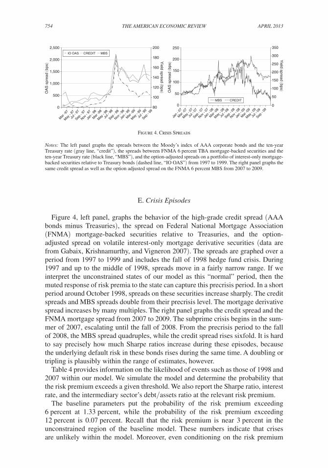
Figure 4, left panel, graphs the behavior of the high-grade credit spread (AAA bonds minus Treasuries), the spread on Federal National Mortgage Association (FNMA) mortgage-backed securities relative to Treasuries, and the option-adjusted spread on volatile interest-only mortgage derivative securities (data are from Gabaix, Krishnamurthy, and Vigneron 2007). The spreads are graphed over a period from 1997 to 1999 and includes the fall of 1998 hedge fund crisis. During 1997 and up to the middle of 1998, spreads move in a fairly narrow range. If we interpret the unconstrained states of our model as this “normal” period, then the muted response of risk premia to the state can capture this precrisis period. In a short period around October 1998, spreads on these securities increase sharply. The credit spreads and MBS spreads double from their precrisis level. The mortgage derivative spread increases by many multiples. The right panel graphs the credit spread and the FNMA mortgage spread from 2007 to 2009. The subprime crisis begins in the sum-mer of 2007, escalating until the fall of 2008. From the precrisis period to the fall of 2008, the MBS spread quadruples, while the credit spread rises sixfold. It is hard to say precisely how much Sharpe ratios increase during these episodes, because the underlying default risk in these bonds rises during the same time. A doubling or tripling is plausibly within the range of estimates, however.

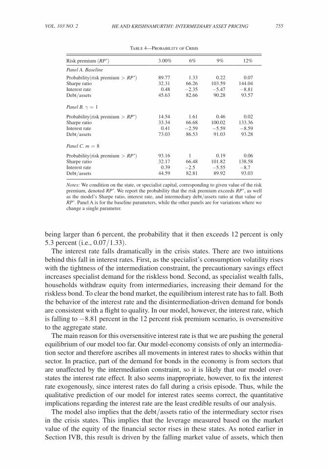
Table 4 provides information on the likelihood of events such as those of 1998 and 2007 within our model. We simulate the model and determine the probability that the risk premium exceeds a given threshold. We also report the Sharpe ratio, interest rate, and the intermediary sector’s debt/assets ratio at the relevant risk premium.

The baseline parameters put the probability of the risk premium exceeding 6 percent at 1.33 percent, while the probability of the risk premium exceeding 12 percent is 0.07 percent. Recall that the risk premium is near 3 percent in the unconstrained region of the baseline model. These numbers indicate that crises are unlikely within the model. Moreover, even conditioning on the risk premium

Figure 4. Crisis Spreads

Notes: The left panel graphs the spreads between the Moody’s index of AAA corporate bonds and the ten-year Treasury rate (gray line, “credit”), the spreads between FNMA 6 percent TBA mortgage-backed securities and the ten-year Treasury rate (black line, “MBS”), and the option-adjusted spreads on a portfolio of interest-only mortgage-backed securities relative to Treasury bonds (dashed line, “IO OAS”) from 1997 to 1999. The right panel graphs the same credit spread as well as the option adjusted spread on the FNMA 6 percent MBS from 2007 to 2009.

Sep -

99

Mar

-97

May

- 97

Jul -

97

Sep -

97Nov

- 97

Jan

- 98

Mar

-98

May

- 98

Jul -

98

Sep -

98Nov

- 98

Jan

- 99

Mar

-99

May

- 99

Jul -

99

80

100

120

140

160

180

200

0

500

1,000

1,500

2,000

2,500

Yield spread (bps)O

AS

spr

ead

(bps

)

IO OAS CREDIT MBS

–

–

–

–

–

–

–

–

–

–

–

–

–– – – – – – – – – – – – – – – – –

0

50

100

150

200

250

300

350

0

50

100

150

200

250Y

ield spread (bps)

OA

S s

prea

d (b

ps)

Sep -

09

Mar

-07

May

- 07

Jul -

07

Sep -

07Nov

- 07

Jan

- 08

Mar

-08

May

- 08

Jul -

08

Sep -

08Nov

- 08

Jan

- 09

Mar

-09

May

- 09

Jul -

09

Jan

- 07

MBS CREDIT

–

–

–

–

–

–

–

––

–

–

–

–

– – – – – – – – – – – – – – – – ––


being larger than 6 percent, the probability that it then exceeds 12 percent is only 5.3 percent (i.e., 0.07/1.33).

The interest rate falls dramatically in the crisis states. There are two intuitions behind this fall in interest rates. First, as the specialist’s consumption volatility rises with the tightness of the intermediation constraint, the precautionary savings effect increases specialist demand for the riskless bond. Second, as specialist wealth falls, households withdraw equity from intermediaries, increasing their demand for the riskless bond. To clear the bond market, the equilibrium interest rate has to fall. Both the behavior of the interest rate and the disintermediation-driven demand for bonds are consistent with a flight to quality. In our model, however, the interest rate, which is falling to −8.81 percent in the 12 percent risk premium scenario, is oversensitive to the aggregate state.

The main reason for this oversensitive interest rate is that we are pushing the general equilibrium of our model too far. Our model-economy consists of only an intermedia-tion sector and therefore ascribes all movements in interest rates to shocks within that sector. In practice, part of the demand for bonds in the economy is from sectors that are unaffected by the intermediation constraint, so it is likely that our model over-states the interest rate effect. It also seems inappropriate, however, to fix the interest rate exogenously, since interest rates do fall during a crisis episode. Thus, while the qualitative prediction of our model for interest rates seems correct, the quantitative implications regarding the interest rate are the least credible results of our analysis.

The model also implies that the debt/assets ratio of the intermediary sector rises in the crisis states. This implies that the leverage measured based on the market value of the equity of the financial sector rises in these states. As noted earlier in Section IVB, this result is driven by the falling market value of assets, which then

Table 4—Probability of Crisis

Risk premium (R P * ) 3.00% 6% 9% 12%

Panel A. Baseline

Probability(risk premium > R P * ) 89.77 1.33 0.22 0.07Sharpe ratio 32.31 66.26 103.59 144.04Interest rate 0.48 −2.35 −5.47 −8.81Debt/assets 45.63 82.66 90.28 93.57

Panel B. γ = 1

Probability(risk premium > R P * ) 14.54 1.61 0.46 0.02Sharpe ratio 33.34 66.68 100.02 133.36Interest rate 0.41 −2.59 −5.59 −8.59Debt/assets 73.03 86.53 91.03 93.28

Panel C. m = 8

Probability(risk premium > R P * ) 93.16 1 0.19 0.06Sharpe ratio 32.17 66.48 101.82 138.58Interest rate 0.39 −2.5 −5.55 −8.7Debt/assets 44.59 82.81 89.92 93.03

Notes: We condition on the state, or specialist capital, corresponding to given value of the risk premium, denoted R P * . We report the probability that the risk premium exceeds R P * , as well as the model’s Sharpe ratio, interest rate, and intermediary debt/assets ratio at that value of RP * . Panel A is for the baseline parameters, while the other panels are for variations where we change a single parameter.


leads to a falling market value of equity (i.e., assets minus debts), which in turn drives up leverage.

Panels B and C provide results for the two variations of the model. The most interesting variation is in panel B, where we report results for the γ = 1 case. We find that the probabilities of the risk premium exceeding R P * are higher in this case than the baseline. Note that this is despite the fact that the average risk premium in the γ = 1 case is lower than that of the γ = 2 case (see Table 3). This is due to the “risk-taking” effect we have alluded to earlier. If we interpret the comparative static of going from γ = 1 to γ = 2 as akin to increasing the average capital requirements on banks, then this result indicates that higher capital requirements can reduce the probability of a crisis. Doubling capital requirements roughly halves the probabili-ties of the 9 percent and 12 percent crisis-states. Panel C indicates that allowing the intermediaries to raise more equity capital from households by increasing m reduces the probability of crises, consistent with intuition.

F. Capital Movement and Recovery from Crisis

Referring to Figure 4, left panel, the corporate bond spread and MBS spread widen from 90 basis points (bps) in July 1998 to a high of 180 bps in October 1998 before coming down to 130 bps in June 1999. Thus, the half-life—that is, the time it takes the spread to fall halfway to the precrisis level—is about 10 months. The interest-only mortgage derivative spread, which is very sensitive to market condi-tions, widens from 250 bps in July 1998 to a high of 2,000 bps before coming back to 500 bps in June 1999. In the right panel, the MBS spread recovers back to its precrisis level by June 2009, while the credit spread remains elevated through the end of the period. We note that this timescale for mean reversion, on the order of months, is much slower than the daily mean-reversion patterns commonly addressed in the market microstructure literature (e.g., Campbell, Grossman, and Wang 1993).

A common wisdom among many observers is that this pattern of recovery reflects the slow movement of capital into the affected markets (Duffie 2010). Our model captures this slow movement. We will show in this section that our baseline calibra-tion can also replicate these speeds of capital movement.

In the crisis states of our model, risk premia are high and the specialists hold lev-eraged positions on the risky asset. Over time, profits from this position increase w t , thereby increasing the capital base of the intermediaries. The increase in specialist capital is mirrored by an m-fold increase in the allocation of households’ capital to the intermediaries. Together these forces reflect a movement of capital back into the risky asset market, leading to increased risk-bearing capacity and lower risk premia. Note, however, that one dimension of capital movement that plausibly occurs in practice but is not captured by our model is the entry of “new” specialists into the risky asset market.

We can use the model simulation to gauge the length and severity of a crisis within our model. Table 5 presents data on how long it takes to recover from a crisis in our model. We fix a state (x, D) corresponding to an instantaneous risk premium in the “Transit from” row. Simulating the model from that initial condition, we compute and report the first passage time that the state hits the risk premium corresponding to the “Transit to” column. The time is reported in years.


Consider panel A, which corresponds to the baseline parameters. If we start from the extreme crisis state of 12 percent and compute how long it takes to recover to 7.5 percent—i.e., halfway back to the unconditional average levels we report earlier of around 3 percent—the time is 0.65 years (7.9 months). From the 10 percent crisis state to the 6.5 percent state (halfway to 3 percent) takes 0.93 years (this number is not reported in the table). For the fall of 1998 episode, the half-life we suggested was around 10 months. The model half-life from 10 percent is of the same order of magnitude as the empirical observation.

Panel B is for the γ = 1 case, fixing the same crisis states measured by the risk pre-mium. Recovery times are faster in this case because a less risk-averse intermediary sector takes on more risk to reach the same risk premium. Essentially, for the same risk premium across panel A and B, the intermediary sector in panel B holds a riskier portfolio and thus earns higher profits from its portfolio. Additionally, the unconditional average risk premium in the γ = 1 case is 2.35 percent compared to the 3.36 percent of the baseline. Thus, even at a risk premium of 3.5 percent, the economy in panel B is still recovering from the crisis.

Panel C is for the m = 8 case. Here also we find faster recovery times. The reason is that specialist capital growth leads to more injections of household capital for a higher m.

The slow adjustment of risk premia, in timescales of many months, during the 1998 episode is also consistent with other studies of crisis episodes. Berndt et al. (2005) study the credit default swap market from 2000 to 2004 and note a dramatic market-wide increase in risk premia (roughly a quadrupling) in July 2002 (see Figures 1 and 2 of the paper). Risk premia gradually fall over the next two years: from the peak in July 2002, risk premia halve by April 2003 (nine months). The authors argue that dislocations beginning with the Enron crisis led to a decrease in risk-bearing capacity among corporate bond investors. Mirroring the decreasing risk-bearing capacity, risk premia rose before slowly falling as capital moved back into the

Table 5—Crisis Recovery

Panel A. Baseline

Transit to 10 7.5 6 5 4 3.5Transit time from 12 0.18 0.65 1.42 2.67 5.56 9.34Increment time 0.18 0.47 0.77 1.25 2.90 3.78

Panel B. γ = 1

Transit time from 12 0.12 0.37 0.71 1.15 2.02 2.85Increment time 0.12 0.25 0.34 0.43 0.88 0.82

Panel C. m = 8

Transit time from 12 0.16 0.60 1.31 2.41 5.28 8.78Increment time 0.16 0.44 0.71 1.10 2.87 3.49

Notes: This table presents transition time data from simulating the model. We fix a state cor-responding to an instantaneous risk premium of 12 percent (“Transit from”). Simulating the model from that initial condition, we compute and report the first passage time that the state hits the risk premium corresponding to that in the “Transit to” row. Time is reported in years. The row “Increment time” reports the time between incremental “Transit to” rows. Data is pre-sented for the baseline parameters and two variations.


corporate bond market and expanded risk-bearing capacity. Gabaix, Krishnamurthy, and Vigneron (2007) note a dislocation in the mortgage-backed securities in late 1993 triggered by an unexpected wave of consumer prepayments. A number of important hedge fund players suffered losses and went out of business during this period, lead-ing to a reduction in risk-bearing capacity. Figure 3 in the paper documents that risk premia reached a peak in December 1993 before halving by April 1994 (five months). Froot and O’Connell (1999) study the catastrophe insurance market and demonstrate similar phenomena. When insurers suffer losses that deplete capital they raise the price of catastrophe insurance. Prices then gradually fall back to long-run levels as capital moves back into the catastrophe insurance market. Froot and O’Connell (1999) show that the half-life in terms of prices can be well over a year.16

Each of these markets are intermediated markets that fit our model well. Investors are institutions who have specialized expertise in assessing risk in their markets. Our theory explains the slow movement of risk-bearing capacity and risk premia documented in these case studies. The calibrated model also captures the frequency of the slow adjustment of risk premia.

V. Crisis Policy Experiments

We study the effect of policy interventions in the crisis of the model. We study three policies: (i) lowering borrowing rates to the intermediary, as with a decrease in the central bank’s discount rate; (ii) direct purchase of the risky asset by the gov-ernment, financed by debt issuance and taxation of households; and (iii) infusing equity capital into the intermediaries during a crisis. These three policies are chosen because they are among those undertaken by central banks in practice. Our aim is to quantify the effects of these policies based on our model. The analysis is purely positive, and we make no claims as to welfare.

Our policy experiments correspond to the following exercise. Suppose we are in a crisis state currently, with a given asset/liability position for the households and specialists. From this initial condition, suppose that the government conducts a policy that was not anticipated by the agents. We trace the effects of this policy on the recovery of the economy from that crisis state.17

To be more precise, we compute two equilibria: one without the policy (which is the equilibrium we have studied thus far), and one with the policy. For example, the first policy that we consider is giving the intermediary sector a borrowing subsidy as long as the economy is in the constrained region. Under such a policy, we can write the subsidy as a function of the primitive state variables and solve the with- policy equilibrium of our model. We then consider the following thought experiment. Suppose that the economy is currently in a given crisis state of the no-policy

16 Mitchell, Pedersen, and Pulvino (2007) document similar effects in the convertible bond market in 1998 and again in 2005. In both cases, crisis recovery times are in the order of months. They also note that spreads in merger arbitrage strategies took several months to recover following the October 1987 risky asset-market crash. Duffie (2010) discusses these and other cases in his presidential address to the American Finance Association.

17 The government policy is a zero-probability event in our exercise. Another experiment would be to study a policy that is expected to be enacted given some value of the state variable—say the government infuses equity capital if the risk premium touches 12 percent. Such a policy would be anticipated by agents within the equilibrium of the model. Analyzing such a policy does not pose any difficulty for our modeling structure, but it adds an extra layer of complexity. For the sake of brevity, we have opted to focus on the simpler experiment.


equilibrium (12 percent risk premium state in the simulations). The government announces the policy, which is unanticipated by agents, and its action causes asset prices to jump immediately. From that point on, the dynamics of the economy are described by the solution to our model under the with-policy equilibrium.18

A. Borrowing Subsidy

During financial crises, the central bank lowers its discount rate and its target for the overnight interbank interest rate. Financial intermediaries rely heavily on rolling over one-day loans for their operation (see, for example, Adrian and Shin 2010 on the overnight repurchase market). Because of this dependence, intermediaries are perhaps the most sensitive sector within the economy to overnight interest rates. Commercial and investment banks have access to overnight funds at the discount window of the central bank. Thus, to the extent that the central bank lowers over-night rates, including the discount rate, it reduces the borrowing costs of financial intermediaries.

While our model does not have a monetary side within which to analyze how a central bank alters the equilibrium overnight interest rate, we can go some way toward examining the effect of this policy by studying the following transfer. The debt position of intermediaries at date t is ( α t I − 1) w t . Suppose that the government makes a lump sum transfer of Δr × ( α t I − 1) w t dt from households to intermediar-ies, where the constant Δr measures the size of the transfer. The transfer is propor-tional to the debt of the intermediary.

The subsidy experiment can be thought of as a reduction in the central bank’s dis-count rate. In practice, when the central bank makes funds available more cheaply to the financial sector through the discount window, it can be viewed as transferring real resources from tax-paying households to the financial sector.

Formally, we examine the policy in which the subsidy Δr is provided to the intermediaries as long as the economy is in the constrained region. That is, Δr is paid only if x < x c , and there is no subsidy if x > x c . We express this transfer of Δr × ( α t I − 1) w t dt in terms of the primitive state variables x t and D t . Then, the dynamic budget constraints of household and specialist are altered to account for the transfer (see equation (11)), and this change is traced through to rederive the ordinary differential equation for the price/dividend ratio (see the online Appendix for details).

Table 6 presents the results for the baseline parameters. We start the economy in the state corresponding to the 12 percent risk premium. The table reports the recovery times from the 12 percent extreme crisis state for different levels of Δr. Consistent with intuition, a higher subsidy speeds up the recovery process. The 200 bps subsidy speeds up the recovery to 7.5 percent by 0.57 years. Note that from August 2007 to October 2008, the discount rate decreased by 450 bps. The last col-umn in the table indicates the effect of this policy within our model.

18 The initial condition from which we simulate the with-policy equilibrium is chosen to match the portfolio holdings of the household in the 12 percent risk premium state of the no-policy equilibrium.


B. Direct Asset Purchase

In both the subprime crisis as well as the Great Depression the government entered the asset market directly to purchase distressed assets. The Federal Reserve and gov-ernment-sponsored enterprises (GSEs) purchased nearly $1.8 trillion of mortgage-backed securities over the period from August 2007 to August 2009 ($1.25 trillion by the Federal Reserve and $550 billion by the GSEs). We can evaluate the impact of this policy as follows. Suppose that the government purchases a fraction s of the risky asset in states x < x c , financing this purchase by issuing s P t of short-term debt (recall that P t is the price of the risky asset). The cash flow from this transaction is s P t (d R t − r t dt ), and we assume that the government raises lump sum taxes from (or rebates to) the households to balance this cash flow.

Table 7 reports the results for three values of s, which is the share of the inter-mediated risky asset market that the government purchases. If we take the stock of intermediated assets to be $15 trillion, then the $1.8 trillion number cited above is 12 percent of this stock. We assume that the policy is initiated in the state corre-sponding to 12 percent risk premium and not removed until the economy recovers back to the unconstrained region. We trace the recovery path from this state.

Table 6—Borrowing Subsidy

Transit to Δr = 0 Δr = 0.01 Δr = 0.02 Δr = 0.045

10.85% 9.82% 7.94%10.00% 0.18 0.08 7.50% 0.65 0.45 0.18 0.086.00% 1.42 1.04 0.65 0.375.00% 2.67 1.85 1.42 0.704.00% 5.56 3.74 2.67 1.29

Notes: This table presents transition time data from simulating the model. We begin in the 12 percent risk premium state and report the first passage time for the state to reach that in the first column of the table (“Transit to” column). Time is reported in years. We report the case of no subsidy (Δr = 0), as well as subsidies of 0.01, 0.02, and 0.045. A subsidy of 0.01 cor-responds to 100 bps. The first row of the table reports the instantaneous jump downward in the risk premium when the government initiates the policy. The simulation is for the baseline parameters.

Table 7—Asset Purchase

Transit to s = 0 s = 0.04 s = 0.08 s = 0.12

11.43% 10.85% 10.25%10.00% 0.18 0.14 0.10 0.057.50% 0.65 0.61 0.58 0.526.00% 1.42 1.39 1.32 1.275.00% 2.67 2.51 2.48 2.404.00% 5.56 5.50 5.48 5.37

Notes: This table presents transition time data from simulating the model. We begin in the 12 percent risk premium state and report the first passage time for the state to reach that in the first column of the table (“Transit to” column). Time is reported in years. We report the case of no purchase (s = 0), as well as purchases of 0.04, 0.08, and 0.12. A purchase with s = 0.04 corresponds to the government buying 4 percent of the outstanding stock of intermediated risky assets. The first row of the table reports the instantaneous jump downward in the risk pre-mium when the government begins its purchase.


The policy causes a downward jump in the risk premium. The asset purchase policy indirectly increases the household’s exposure to the risky asset because future taxes now depend on the returns to the risky asset. In turn, this means that specialists bear less risk in equilibrium and hence the risk premium falls. Effectively, this policy puts less risk on the limited risk-bearing capacity of the intermediary sector. After this initial jump the recovery path is almost the same as the case of no intervention. For example, if we compare the incremental time it takes the economy to move from 7.5 percent to 6 percent, we see that the time for the no intervention case is 0.76 years, while it is 0.73 years for the case of s = 0.12. Intuitively, the purchase has no further effect because of the following countervailing force. The specialist holds a smaller position in the risky asset, as the taxpayer holds a larger share. Hence, less of the risk premium accrues to the intermediary capital, leading to a slower recovery.

C. Capital Infusion

A number of crisis interventions are aimed at increasing the equity capital of inter-mediaries. For example, in the Great Depression, the government directly acquired preferred shares in banks, thereby increasing their equity capital. In the subprime crisis, the US Treasury purchased $205 billion of preferred shares in the intermedi-ary sector through the capital purchase program.

We examine a policy in which m is increased to _ m > 4 in the constrained region

with x < x c . The higher m indicates that the intermediary increases its equity capital proportionate to

_ m − m. The extra equity capital is purchased by the government, and paid for by lump sum taxes on the households. Returns on the government investment are rebated in a lump sum fashion to the households. We think of the increase in m as a temporary relaxation of the equity capital constraint. For example, one may imagine that the government is temporarily able to monitor intermediaries better than households during a crisis and can thus relax the capital constraint. Our aim is to quantify the effect of the relaxation of the constraint on the crisis recovery.

We choose _ m to represent the Treasury’s purchase of $205 billion of bank capi-

tal. Note that capital in our model refers to common shares, while in practice, the Treasury purchased preferred shares. The distinction is important because our model works through the sharing of risk between the specialist and the household/government, rather than directly through the amount of funds that are transferred to the intermediary sector. When the government invests in the intermediary and shares some of the risk in the specialist’s investment, the specialist bears less risk in equilibrium and the risk premium adjusts downward. The returns on common shares are more sensitive to the returns on intermediary investment than are the returns on preferred shares, indicating that common shares allow for more risk sharing than preferred shares. Franks and Torous (1994), based on a sample of distressed firms over the period 1983 to 1988, document that in a bankruptcy/reorganization, pre-ferred shares are repaid 42 percent of face value.19 We translate the preferred share

19 In our model, the value of common shares approaches zero as the value of assets falls towards the value of liabilities (the bankruptcy threshold). Likewise, as the value of assets rises, preferred shares received a relatively fixed dividend, while the value of common shares increases.


purchase in terms of common shares using the 42 percent number of Franks and Torous (1994); that is, we assume that an injection of $1 of preferred shares is equal to an injection of $0.58 (= 1 − 0.42) of common shares.

The Treasury’s capital injection was distributed across many banks, from pure lending institutions to trading institutions. Since our model is primarily about securities markets and trading institutions, we apportion the $205 billion of capi-tal to reflect the injection of capital to support securities trading. We multiply the injection by 0.40, which is the fraction of securities in total bank assets, as com-puted from the Flow of Funds 2007 data, to give an equity injection of $48 billion (= 205 × 0.58 × 0.40). Finally, we interpret the government’s equity injection as an increase of the specialist’s inside capital that is then matched by a fourfold increase in capital from households. That is, we interpret the events of 2008–2009 as, first, the government does the troubled asset relief program, and, second, this enabled the financial sector to raise further equity from private investors.

Within the model we evaluate the effect of raising m to _ m in the crisis states,

where _ m is chosen so that the implied increase in specialist equity capital (as a frac-

tion of total assets under intermediation) in the 12 percent crisis state is 1.6 percent (i.e., 5 × $48 billion divided by $15 trillion). The equity-asset ratio of the interme-

diary sector in the constrained region is ( 1 + m ) w

_ P . We choose _ m so that

( 1 + _ m ) w _ P −

( 1 + m ) w _ P is equal to 1.28 percent, based on the w and P of the no-policy equilibrium

in the 12 percent risk premium state. The results are in Table 8. We also present results for a $38 billion and $58 billion equity injection.

The effects of policy are qualitatively similar to the other cases: there is a jump downward in the risk premium and a gradual adjustment afterward. It is most interesting to compare the effects of the three policies. Compared to the asset purchase case, we see that a relatively small amount of funds used toward equity purchase produces a much faster recovery. The reason that the equity injection has such a large effect is that the fundamental friction in our model is an equity capital constraint. The equity capital injection of $48 billion, corresponding to the actual policy enacted in 2008–2009, leads to a recovery time to the 6 percent state of 1.10 years. Compare this to the asset purchase policy, where buying $1.8 tril-lion of assets leads a recovery time of 1.27 years. Finally, the 450 bps borrowing

Table 8—Equity Injection

Transit to Baseline $38 billion $48 billion $58 billion

9.57% 9.05% 8.57%10.00% 0.187.50% 0.65 0.43 0.37 0.276.00% 1.42 1.19 1.10 0.995.00% 2.67 2.35 2.24 2.144.00% 5.56 5.23 5.01 4.95

Notes: This table presents transition time data from simulating the model. We begin in the 12 percent risk premium state and report the first passage time for the state to reach that in the first column of the table (“Transit to” column). Time is reported in years. We report the case of a purchase of equity capital of $38 billion, $48 billion, and $58 billion, which is reversed in roughly one year. The first row of the table reports the instantaneous jump downward in the risk premium when the government injects the equity capital.


subsidy, corresponding to actual policy, leads to the fastest recovery time of 0.37 years. This policy has a large effect because the intermediaries are very lever-aged in our model, carrying a debt/asset ratio of 94 percent in the 12 percent risk premium state. These numbers concern the benefits of these policies. To provide a more comprehensive assessment of the policies, one also needs to evaluate the costs of these interventions.

VI. Conclusion

We have presented a model to study the dynamics of risk premia in a crisis episode where intermediaries’ equity capital is scarce. We calibrate the model and show the model does well in matching two aspects of crises: the nonlinearity of risk premia in crisis episodes, and the recovery from crises in the order of many months. We also use the model to evaluate the effectiveness of central bank poli-cies, finding that infusing equity capital into intermediaries is the most effective policy in our model.

A limitation of our model is that it does not shed any light on the connection between the performance of intermediated asset markets we model (i.e., the mort-gage-backed securities market) and the stock market. Yet, as we have seen dur-ing the subprime crisis, the deterioration in intermediation does spill over to the S&P 500. In He and Krishnamurthy (2013) we develop a related model with capital accumulation whereby the deterioration in intermediation affects capital investment and output. The model thus takes a step in the broader direction of integrating the capital market and real investment into our framework.

Mathematical Appendix

A. ODE Solution

We detail the ODE that characterizes the equilibrium. In the main text we use x, which is the ratio of the specialist’s wealth w to the price of risk asset price P, as the state variable. In writing down the ODE, it turns out the expressions are simpler by changing variables to an alternative state variable y ≡ w h /D, which is households’ wealth w h scaled by the current dividend level D. Denote the price-dividend ratio with the alternative state variable as F ( y ) . Once we solve for the equilibrium price-dividend ratio F ( y ) , we can convert back to the original state variable x by

(A1) x = 1 − y/F ( y ) ,

and the price-dividend ratio p ( x ) as a function of the fraction of specialists’ wealth x satisfies

F ( y ) = p ( 1 − y/F ( y ) ) .

When x ranges from 0 to 1, y takes value from F ( y b ) to 0, where the maximum households wealth y b = 1 + l

_ ρ as discussed in the text.


Denote the dynamics of y t as

(A2) d y t = μ y dt + σ y d Z t ,

for unknown functions μ y and σ y . We write d c t _ c t and d R t as functions of μ y , σ y , and

the derivatives of F ( y ) . Due to market clearing, c t = D t ( 1 + l − ρ y t ) (the simple expression for the equilibrium specialist’s consumption is the reason why we work with the new state variable y), thus we have

d c t _ c t =

d D t _ D t −

ρdy _

1 + l − ρy −

ρ _

1 + l − ρy Co v t [ dy, dD _

D ]

= ( g − ρ _

1 + l − ρy ( μ y + σ y σ ) ) dt + ( σ −

ρ σ y _

1 + l − ρy ) d Z t .

We also have

d R t = d P t + D t dt

_ P t

= [ g + F′ _ F

μ y + 1 _ 2 F″ _

F σ y 2 + 1 _

F + F′ _

F σ y σ ] dt + ( σ + F′ _

F σ y ) d Z t .

Substituting these expressions into equation (15), we obtain the following ODE:

(A3) g + F′ _ F

( μ y + σ y σ ) + 1 _ 2 F″ _

F σ y 2 + 1 _

F = ρ + γ g

− γρ _

1 + l + ρy ( μ y + σ y σ )

+ γ ( σ − ρ σ y _

1 + l + ρy ) ( σ +

F′ σ y _

F )

− γ (γ + 1)

_ 2 ( σ −

ρ σ y _

1 + l + ρy ) 2 .

Derivation of μ y and σ y .—We rewrite equation (11), which describes the wealth dynamics (budget constraint) of the household sector, as

(A4) d w h = θ s dP + D θ s dt + r θ b Ddt + l D t dt − ρ w h dt.

In this equation,

(A5) θ s = α I α h (1 − λ) w h _ P

are the number of shares that the risky asset household owns, and

(A6) θ b D = w h − θ s P


is the amount of funds that the households have invested in the riskless bond, which includes the direct investment of debt households, the investment of risky asset households (when constraint is binding), and the indirect investment through inter-mediaries who short on bond in equilibrium. The portfolio choices α h and α I are defined in Section IIB in the main text and depend on whether the economy is con-strained or not. Note that we have θ b + F ( y ) θ s = y from equation (A6).

We apply Ito’s Lemma to P = DF(y ) to find expressions for the drift and diffu-sion of dP. We can then substitute back into equation (A4) to find expressions for the drift and diffusion of d w h .

Also, recall that we have defined w h = Dy. We apply Ito’s Lemma to this equa-tion to arrive at a second expression for the drift and diffusion of d w h . Matching the drift and diffusion terms from these two ways of writing d w h , we solve to find μ y and σ y .

The result of this algebra is that

σ y = − θ b _

1 − θ s F′ σ,

and

(A7) μ y + σ σ y = 1 _ 1 − θ s F′

( θ s + l + (r − g ) θ b − ρy + 1 _ 2 θ s F″ σ y 2 ) .

ODE.—Substituting for μ y + σ σ y derived in equation (A7) into equation (A3), we find

( F′ _ F

+ γρ _

1 + l − ρy ) ( 1 _

1 − θ s F′ ) ( θ s + l + θ b (r − g ) − ρ y )

+ 1 _ F

+ 1 _ 2 F″ σ y 2 ( 1 _

1 − θ s F′ ) ( 1 _

F + θ s

γρ _

1 + l − ρy )

= ρ + g(γ − 1) + γ ( σ − ρ _

1 + l − ρy σ y ) ( σ + F′ _

F σ y )

− 1 _ 2 γ (γ + 1 ) ( σ −

ρ _

1 + l − ρy σ y ) 2 ,

where the endogenous interest rate r is determined by the following equation:

r = ρ + gγ − ργ _

1 + l − ρy

θ s + l + ( r − g ) θ b − ρy + σ 2 _

2 θ s F″

θ b 2 _

( 1 − θ s F′ ) 2

____ 1 − θ s F′

− γ ( γ + 1 ) σ 2

_ 2 ( 1 +

ρ θ b _ 1 + l − ρy

1 _ 1 − θ s F′

) 2 .


We define a function, G(y ) ≡ 1 _

1 − θ s F′ , and hence σ y = − θ b _

1 − θ s F′ σ = − θ b σG.

Therefore we can rewrite our ODE as

F″ θ s G 2 ( θ b σ ) 2

_ 2 G ( 1 _

θ s F +

γρ _

1 + l − ρy )

= ρ + g (γ − 1) − 1 _ F

+ 1 _ 2 γ σ 2 ( 1 +

ρ _

1 + l − ρ y θ b G )

× ( 2 ( y − G θ b ) _

θ s F − ( 1 + γ )

1 + l − ρ y + ρ G θ b __ 1 + l − ρ y

) − ( G − 1 _

θ s F +

γρ _

1 + l − ρ y G ) ( θ s + l + θ b (r − g) − ρ y ) ,

and solve for r as

r = 1 _ 1 +

ρ γ G θ b _

1 + l − ρ y [ρ + g γ −

ρ γ G _

1 + l − ρ y ( θ s + l − g θ b − ρ y + σ 2 _

2 θ s G 2 F″ θ b 2 )

− γ ( γ + 1 ) σ 2

_ 2 ( 1 +

ρ θ b G _

1 + l − ρ y ) 2 ].

We combine these two pieces, use the relation θ b = y − θ s F and θ b ( G − 1 _ θ s F

+ γ ρ G _

1 + l − ρy )

= − y − G θ b _ θ s F

+ 1 + l − ρ y + γρ G θ b _

1 + l − ρ y , and arrive at the final expression of the ODE:

(A8) F″ θ s G 2 ( θ b σ ) 2

_ 2

G _

θ s F ( 1 + l + ρ y (γ − 1)

__ 1 + l − ρ y + ρ γ G θ b

)

= ρ + g (γ − 1) − 1 _ F +

γ ( 1 − γ ) σ 2 _

2 ( 1 + ρ G θ b

_ 1 + l − ρ y

) y − G θ b _

θ s F [ 1 + l − ρ y − ρ G θ b

__ 1 + l − ρ y + ρ γ G θ b

]

− ( ( 1 + l − ρ y ) ( G − 1 ) __

θ s F + γ ρ G ) θ s + l + θ b (g (γ − 1) + ρ) − ρ y

__ 1 + l − ρ y + ρ γ G θ b

.

The expressions for the bond holding θ b and risky asset holding θ s depend on whether the economy is constrained or not. In the unconstrained region, as shown in Section IIB, α h = 1, and α I = 1

_ x + ( 1 − λ ) ( 1 − x ) = F

_ F − λy

using equation (A1).

Utilizing equations (A6) and (A5), we have θ s = ( 1 − λ ) y _

F − λy , and θ b = λy

F − y _

F − λy .


In the constrained region α h = m _

1−λ x _ 1−x = m ( F−y )

_ ( 1−λ ) y , α I = 1 _ 1 + m 1 _ x = 1

_ 1 + m F _ F − y ,

therefore θ s = m _ 1 + m , and θ b = y − m

_ 1 + m F. Finally, as illustrated in Section IIB,

the cutoff for the constraint satisfies 1 _ x c

= 1 + m _

1−λ . Translating to y, we have y c = m

_ 1−λ+m

F( y c ), and the economy is in the unconstrained region if 0 < y ≤ y c .

B. Boundary Conditions and Technical Parameter Restriction

The upper boundary condition is described in Section IID. A lower boundary condition occurs when y → 0. This case corresponds to one where specialists hold the entire financial wealth of the economy. Using L’Hopital’s rule, it is easy to check

that G − 1 _ θ s F

→ F′ ( 0 ) _

F ( 0 ) . Plugging this result into equation (A8), and noting that both θ s and θ b go to zero as y goes to zero, we obtain

(A9) F ( 0 ) = 1 + F′ ( 0 ) l

___ ρ + g (γ − 1) +

γ ( 1 − γ ) σ 2 _

2 −

lγρ _

1 + l

.

When l = 0, one can check that F ( 0 ) is the equilibrium price-dividend ratio for the economy with the specialists as the representative agent. Because in our model the growth of the household sector affects the pricing kernel, however, this boundary P/D ratio F ( 0 ) also depends on the household’s labor income l. For the P/D ratio to be well defined at y = 0 (and, thus, at x = 1), we require that parameters satisfy

ρ + g (γ − 1) + γ ( 1 − γ ) σ 2

_ 2 −

lγρ _

1 + l > 0.

Furthermore, a straightforward calculation yields that F ′ ( y b ) = 1 if F ( y b ) = y b . This result also ensures that at the boundary y b the mapping from the scaled house-hold’s wealth y to the fraction of the specialists’ wealth x = w/P = 1 − y/F ( y ) is monotonely decreasing, as x′ ( y ) = ( F ( y ) − yF′ ( y ) ) / F 2 ( y ) attaches zero when y → y b .

Numerical Method.—In our ODE (A8) both boundaries are singular, caus-ing difficulties in directly applying the built-in ODE solver ode15s in Matlab. To overcome this issue, we approximate the upper-end boundary ( y b , F ( y b ) = y b ) by ( y b − η, y b − η ) (where η is sufficiently small), and adopt a “forward-shoot-ing and line-connecting” method for the lower-end boundary. Take a small ϵ > 0 and call ̃ F as the attempted solution. For each trial ϕ ≡ ̃ F ′ ( ϵ ) , we set ̃ F ′ (0) = ϕ, solve ̃ F (0) based on equation (A9), and let ̃ F (ϵ) = ̃ F (0) + ϕϵ. Since ( ϵ, ̃ F ( ϵ ) ) is away from the singularity, by trying different ϕs we apply the stan-dard shooting method to obtain the desired solution F that connects at ( y b − η, y b − η ) . For y < ϵ, we simply approximate the solution by a line connect-

ing ( 0, F ( 0 ) ) and ( ϵ, F ( ϵ ) ) . In other words, we solve F on [ ϵ, y b ] with a smooth


pasting condition for F′ ( ϵ ) = F ( ϵ ) − F ( 0 ) _ ϵ and a value matching condition for

F ( y b ) = y b .We use ϵ = 0.25 and η = 0.001, which give ODE errors bounded by 3 × 1 0 −5

for y > ϵ. Different ϵs and ηs deliver almost identical solutions for y > 1. Because we are mainly interested in the solution behavior near y c (which takes a value of 63.53 in the benchmark case) and onward, our main calibration results are free of the approximation errors caused by the choice of ϵ and η. Finally, we find that, in fact, these errors are at the same magnitude as those generated by the capital con-straint around y c ( 3.5 × 1 0 −5 ) .

Simulation.—With the ODE solutions in hand, we numerically simulate the model to obtain the steady state distribution of the state variable x as well as a number of asset price measurements. We begin the economy at a state ( x 0 = x c , D 0 = 1 ) and simulate the economy for 5,000 years. That is, we obtain a sequence of independent draws from the normal distribution and use these draws to represent innovations in our shock process Z t . The path of Z t can then be mapped into a path of the state vari-able. We compute the time-series averages of a number of relevant asset price mea-surements from years 1,000 to 5,000 of this sample. The simulation unit is monthly, and based on those monthly observations we compute annual averages. We repeat this exercise 5,000 times, averaging across all of the simulated Z t paths. We find that changing the starting value x 0 does not affect the computed distribution or any of the asset price measurements, indicating that the distribution is an accurate representa-tion of the steady state distribution of the economy.

REFERENCES

Adrian, Tobias, and Hyun Song Shin. 2010. “Liquidity and Leverage.” Journal of Financial Interme-diation 19 (3): 418–37.

Adrian, Tobias, Erkko Etula, and Tyler Muir. 2012. “Financial Intermediaries and the Cross-Section of Asset Returns.” Unpublished.

Aiyagari, S. Rao, and Mark Gertler. 1999. “‘Overreaction’ of Asset Prices in General Equilibrium.” Review of Economic Dynamics 2 (1): 3–35.

Allen, Franklin, and Douglas Gale. 2005. “From Cash-in-the-Market Pricing to Financial Fragility.” Journal of the European Economic Association 3 (2–3): 535–46.

Alvarez, Fernando, Andrew Atkeson, and Patrick J. Kehoe. 2002. “Money, Interest Rates, and Exchange Rates with Endogenously Segmented Markets.” Journal of Political Economy 110 (1): 73–112.

Ang, Andrew, Sergiy Gorovyy, and Greg van Inwegen. 2011. “Hedge Fund Leverage.” Journal of Financial Economics 102 (1): 102–26.

Barberis, Nicholas, Ming Huang, and Tano Santos. 2001. “Prospect Theory and Asset Prices.” Quar-terly Journal of Economics 116 (1): 1–53.

BarclayHedge. March 2009. “The Hedge Fund Flow Report.” http:www.barclayhedge.com/research/hedge-fund-flow-report/hedge-fund-flow-report.html (accessed October 2009).

Basak, Suleyman, and Domenico Cuoco. 1998. “An Equilibrium Model with Restricted Stock Market Participation.” Review of Financial Studies 11 (2): 309–41.

Bates, David S. 2003. “Empirical Option Pricing: A Retrospection.” Journal of Econometrics 116 (1–2): 387–404.

Bernanke, Ben, and Mark Gertler. 1989. “Agency Costs, Net Worth, and Business Fluctuations.” American Economic Review 79 (1): 14–31.

Berndt, Antje, Rohan Douglas, Darrell Duffie, Mark Ferguson, and David Schranz. 2005. “Measur-ing Default Risk Premia from Default Swap Rates and EDFs.” Bank for International Settlements Working Paper 173.

Borodin, Andrei N., and Paavo Salminen. 1996. Handbook of Brownian Motion: Facts and Formulae. Boston: Birkhauser Verlag.

www.barclayhedge.com/research/hedge-fund-flow-report/hedge-fund-flow-report.html

www.barclayhedge.com/research/hedge-fund-flow-report/hedge-fund-flow-report.html


Boudoukh, Jacob, Matthew Richardson, Richard Stanton, and Robert Whitelaw. 1997. “Pricing Mort-gage-Backed Securities in a Multifactor Interest Rate Environment: A Multivariate Density Estima-tion Approach.” Review of Financial Studies 10 (2): 405–46.

Brunnermeier, Markus K., and Lasse Heje Pedersen. 2009. “Market Liquidity and Funding Liquidity.” Review of Financial Studies 22 (6): 2201–38.

Brunnermeier, Markus K., and Yuliy Sannikov. 2011. “A Macroeconomic Model with a Financial Sec-tor.” Unpublished.

Campbell, John Y., and John H. Cochrane. 1999. “By Force of Habit: A Consumption-Based Explana-tion of Aggregate Stock Market Behavior.” Journal of Political Economy 107 (2): 205–51.

Campbell, John Y., Sanford J. Grossman, and Jiang Wang. 1993. “Trading Volume and Serial Correla-tion in Stock Returns.” Quarterly Journal of Economics 108 (4): 905–39.

Collin-Dufresne, Pierre, Robert S. Goldstein, and J. Spencer Martin. 2001. “The Determinants of Credit Spread Changes.” Journal of Finance 56 (6): 2177–207.

Diamond, Douglas W., and Philip H. Dybvig. 1983. “Bank Runs, Deposit Insurance, and Liquidity.” Journal of Political Economy 91 (3): 401–19.

Diamond, Douglas W., and Raghuram G. Rajan. 2005. “Liquidity Shortages and Banking Crises.” Journal of Finance 60 (2): 615–47.

Duffie, Darrell. 2010. “Presidential Address: Asset Price Dynamics with Slow-Moving Capital.” Jour-nal of Finance 65 (4): 1237–67.

Duffie, Darrell, and Bruno Strulovici. 2011. “Capital Mobility and Asset Pricing.” National Bureau of Economic Research Working Paper 17296.

Dumas, Bernard. 1989. “Two-Person Dynamic Equilibrium in the Capital Market.” Review of Finan-cial Studies 2 (2): 157–88.

Edmond, Chris, and Pierre-Olivier Weill. 2009. “Aggregate Implications of Micro Asset Market Seg-mentation.” National Bureau of Economic Research Working Paper 15254.

Federal Reserve Board. March 11, 2010. “Flow of Funds Accounts of the United States: Level Tables.” (accessed June 2010).

Fostel, Ana, and John Geanakoplos. 2008. “Leverage Cycles and the Anxious Economy.” American Economic Review 98 (4): 1211–44.

Franks, Julian R., and Walter N. Torous. 1994. “A Comparison of Financial Recontracting in Distressed Exchanges and Chapter 11 Reorganizations.” Journal of Financial Economics 35 (3): 349–70.

Froot, Kenneth A., and Paul G. J. O’Connell. 1999. “The Pricing of U.S. Catastrophe Reinsurance.” In The Financing of Catastrophe Risk, edited by Kenneth A. Froot, 195–227. Chicago: University of Chicago Press.

Fung, William K. H., and David A. Hsieh. 2006. “Hedge Funds: An Industry in Its Adolescence.” Fed-eral Reserve Bank of Atlanta Economic Review 91 (4): 1–34.

Gabaix, Xavier, Arvind Krishnamurthy, and Olivier Vigneron. 2007. “Limits of Arbitrage: Theory and Evidence from the Mortgage-Backed Securities Market.” Journal of Finance 62 (2): 557–95.

Garleanu, Nicolae, Lasse Heje Pedersen, and Allen M. Poteshman. 2009. “Demand-Based Option Pric-ing.” Review of Financial Studies 22 (10): 4259–99.

Gatev, Evan, and Philip E. Strahan. 2006. “Banks’ Advantage in Hedging Liquidity Risk: Theory and Evidence from the Commercial Paper Market.” Journal of Finance 61 (2): 867–92.

Gromb, Denis, and Dimitri Vayanos. 2002. “Equilibrium and Welfare in Markets with Financially Constrained Arbitrageurs.” Journal of Financial Economics 66 (2–3): 361–407.

He, Zhiguo, In Gu Khang, and Arvind Krishnamurthy. 2010. “Balance Sheet Adjustments during the 2008 Crisis.” IMF Economic Review 58 (1): 118–56.

He, Zhiguo, and Arvind Krishnamurthy. 2012. “A Model of Capital and Crises.” Review of Economic Studies 79 (2): 735–77.

He, Zhiguo, and Arvind Krishnamurthy. 2013. “Intermediary Asset Pricing: Dataset.” American Eco-nomic Review. http://dx.doi.org/10.1257/aer.103.2.732.

He, Zhiguo, and Arvind Krishnamurthy. 2013. “A Macroeconomic Framework for Quantifying Sys-temic Risk.” Unpublished.

Holderness, Clifford G., Randall S. Kroszner, and Dennis P. Sheehan. 1999. “Were the Good Old Days that Good? Changes in Managerial Stock Ownership since the Great Depression.”Journal of Finance 54 (2): 435–69.

Holmström, Bengt, and Jean Tirole. 1997. “Financial Intermediation, Loanable Funds, and the Real Sector.” Quarterly Journal of Economics 112 (3): 663–91.

Karatzas, Ioannis, and Steven E. Shreve. 1998. Methods of Mathematical Finance. New York: Springer.Kiyotaki, Nobuhiro, and John Moore. 1997. “Credit Cycles.” Journal of Political Economy 105 (2):

211–48.



Kyle, Albert S., and Wei Xiong. 2001. “Contagion as a Wealth Effect.” Journal of Finance 56 (4): 1401–40.

Lucas, Robert E., Jr. 1978. “Asset Prices in an Exchange Economy.” Econometrica 46 (6): 1429–45.Mankiw, N. Gregory, and Stephen P. Zeldes. 1991. “The Consumption of Stockholders and Nonstock-

holders.” Journal of Financial Economics 29 (1): 97–112.McGuire, Patrick, Eli Remolona, and Kostas Tsatsaronis. 2005. “Time-Varying Exposures and Lever-

age in Hedge Funds.” Bank for International Settlements Quarterly Review, March: 59–72. Mitchell, Mark, Lasse Heje Pedersen, and Todd Pulvino. 2007. “Slow Moving Capital.” American

Economic Review 97 (2): 215–20.Pennacchi, George. 2006. “Deposit Insurance, Bank Regulation, and Financial System Risks.” Journal

of Monetary Economics 53 (1): 1–30.Shleifer, Andrei, and Robert W. Vishny. 1997. “The Limits of Arbitrage.” Journal of Finance 52 (1):

35–55.United States Security and Exchange Commission. 2008, First Quarter.“Form 10-Q.” Filings for Gold-

man Sachs, Morgan Stanley, Merrill Lynch, Citigroup Global Markets, Bank of America Securities, J.P. Morgan, Lehman Brothers, and Bear Stearns (accessed October 2009).

Vayanos, Dimitri. 2004. “Flight to Quality, Flight to Liquidity, and the Pricing of Risk.” National Bureau of Economic Research Working Paper 10327.

Vissing-Jorgensen, Annette. 2002. “Limited Asset Market Participation and the Elasticity of Intertem-poral Substitution.” Journal of Political Economy 110 (4): 825–53.

Wang, Jiang. 1996. “The Term Structure of Interest Rates in a Pure Exchange Economy with Hetero-geneous Investors.” Journal of Financial Economics 41 (1): 75–110.

Xiong, Wei. 2001. “Convergence Trading with Wealth Effects: An Amplification Mechanism in Finan-cial Markets.” Journal of Financial Economics 62 (2): 247–92.

This article has been cited by:

1. Eric van Wincoop. 2013. International Contagion through Leveraged Financial Institutions. AmericanEconomic Journal: Macroeconomics 5:3, 152-189. [Abstract] [View PDF article] [PDF with links]

http://dx.doi.org/10.1257/mac.5.3.152

http://pubs.aeaweb.org/doi/pdf/10.1257/mac.5.3.152

http://pubs.aeaweb.org/doi/pdfplus/10.1257/mac.5.3.152

intermediary asset pricing - booth school of...

Documents