Integrative multivariate distribution models

with generalized hyperbolic margins

Rafael Schmidt 1,2

Department of Statistics, The London School of Economics & Political Science,

London, WC2A 2AE, United Kingdom

Tomas Hrycej, Eric Stutzle 2

Department of Information Mining, DaimlerChrysler AG - Research and

Technology, 89069 Ulm, Germany

Abstract

Multivariate generalized hyperbolic distributions represent an attractive family ofdistributions (with exponentially decreasing tails) for multivariate data modelling.However, in a limited data environment, robust and fast estimation procedures arerare. In this paper we propose an alternative class of multivariate distributions(with exponentially decreasing tails) belonging to affine-linear transformed randomvectors with stochastically independent and generalized hyperbolic margins. Thelatter distributions possess good estimation properties and have attractive depen-dence structures which we explore in detail. In particular, dependencies of extremeevents (tail dependence) can be modelled within this class of multivariate distribu-tions. In addition we introduce the necessary estimation and generation procedures.Various advantages and disadvantages of both types of distributions are discussedand illustrated via a simulation study.

Key words: Multivariate distributions, Generalized hyperbolic distributions,Affine-linear transforms, Copula, Tail dependence, Estimation, Random numbergeneration

Email address: r.schmidt@lse.ac.uk (Rafael Schmidt).URL: http://stats.lse.ac.uk/schmidt/ (Rafael Schmidt).

1 This work was supported by a fellowship within the Postdoc-Programme of the GermanAcademic Exchange Service (DAAD).2 The authors would like to thank Professor Ulrich Stadtmuller for very helpful discussionsand contributions. Further, the authors are grateful to Professor Gholamreza Nakhaeizadeh forsupporting this work.

Preprint submitted to Elsevier Science 2 December 2003

1 Introduction

Data analysis with generalized hyperbolic distributions has become quite popular in vari-ous areas of theoretical and applied statistics. Originally, Barndorff-Nielsen (1977) utilizedthis class of distributions to model grain size distributions of wind-blown sand (cf. alsoBarndorff-Nielsen and Blæsild (1981) and Olbricht (1991)). In econometrical finance thelatter family of distributions has been used for multidimensional asset-return modelling.In this context, the generalized hyperbolic distribution replaces the Gaussian distribu-tion which cannot model the fat tails and the distributional skewness of most financialasset-return data. References are Eberlein and Keller (1995), Prause (1999), Bauer (2000),Bingham and Kiesel (2001), and Eberlein (2001).

Multivariate generalized hyperbolic distributions (in short: MGH distributions) were in-troduced and investigated by Barndorff-Nielsen (1978) and Blæsild and Jensen (1981).These distributions have attractive analytical and statistical properties whereas robustand fast parameter estimations turn out to be difficult in higher dimensions. Further,MGH distribution functions possess no parameter constellation for which they are theproduct of their marginal distribution functions. However, many applications require themultivariate distribution function to model both: Marginal dependence and independence.Because of these and other insufficiencies (see also Section 5) we introduce and explorea new class of multivariate distributions, the so called multivariate affine generalized hy-perbolic distributions (in short: MAGH distributions). This class of distributions has anappealing stochastic representation and, in contrast to the MGH distributions, the esti-mation and simulation algorithms simplify. Moreover, our simulation study reveals thatthe goodness-of-fit of the MAGH distribution is comparable to that of the MGH distribu-tion. The one-dimensional margins of an MAGH distribution are even more flexible dueto more flexibility in the parameter choice.

We show that the dependence structure of an MAGH distribution is appropriate for datamodelling. In particular, the correlation matrix as an important dependence measure ismore intuitive and easier to handle for an MAGH distribution than for an MGH distri-bution. Further, zero correlation implies independent margins of the MAGH distributionwhereas the margins of an MGH distribution do not have this property. Moreover, incontrast to the MGH distributions, the MAGH distributions can model dependencies ofextreme events (so called tail dependence).

On the other hand, MGH distributions embrace a large subclass of distributions whichbelong to the family of elliptically or spherically contoured distributions. The family ofelliptically contoured distributions inherits many useful properties from the multivariatenormal distribution, like closure properties for linear regression and for passing to marginaldistributions (see Cambanis, Huang, and Simons (1981)). Moreover, various tests for sta-tistical inference under the assumption of a normal distribution are also applicable in theelliptical world (see Fang, Kotz, and Ng (1990)). Therefore it also depends on the kind ofapplication which distribution to put in favor.

Sections 2 and 3 introduce the MGH and MAGH distributions and characterize the sub-class of elliptically contoured distributions. In Section 4 we investigate the dependencestructure of both distributions by utilizing the theory of copulae. Section 5 discusses the

2

advantages and disadvantages of the MGH and MAGH distributions. The correspondingestimation and generation algorithms are elaborated in Sections 6 and 7. Finally, in Sec-tion 8, we present a detailed simulation study to illustrate the elaborated results. TheAppendix contains various results and proof mainly relating to the tail behavior of MGHand MAGH distributions.

2 Multivariate generalized hyperbolic model (MGH)

In the first place, a subclass of MGH distributions, namely the hyperbolic distributions,has been introduced via so-called variance-mean mixtures of inverse Gaussian distribu-tions. This subclass suffers from not having hyperbolic distributed margins, i.e., the sub-class is not closed with respect to passing to marginal distributions. Therefore and becauseof other theoretical aspects, Barndorff-Nielsen (1977) extended this class to the family ofMGH distributions. Many different parametric representations of MGH density functionsare provided in the literature, see e.g. Blæsild and Jensen (1981). The following densityrepresentation is appropriate in our context.

Definition 1 (MGH distribution) An n-dimensional random vector X is said to bemultivariate generalized hyperbolic (MGH) distributed with location vector µ ∈ IRn andscaling matrix Σ ∈ IRn×n if it has the following stochastic representation:

Xd= A′Y + µ (1)

for some lower triangular matrix A′ ∈ IRn×n such that A′A = Σ is positive-definite andY possesses the density function

fY (y) = cKλ−n/2(α

√1 + y′y)

(1 + y′y)n/4−λ/2eαβ′y, y ∈ IRn. (2)

The normalizing constant c is given by

c =αn/2 (1 − β′β)λ/2

(2π)n/2Kλ(α√

1 − β′β), (3)

where Kν denotes the modified Bessel-function of the third kind with index ν (cf. Magnus,Oberhettinger, and Soni (1966), pp. 65) and the parameter domain is ‖β‖2 < 1, α > 0and λ ∈ IR (‖ · ‖2 denotes the Euclidian norm). The family of n-dimensional generalizedhyperbolic distributions is denoted by MGHn(µ,Σ, ω), where ω := (λ, α, β).

An important property of the above parameterization of the MGH density function is itsinvariance under affine-linear transformations. For λ = (n + 1)/2 we obtain the multi-variate hyperbolic density and for λ = −1/2 the multivariate normal inverse Gaussiandensity. Hence λ = 1 leads to hyperbolically distributed one-dimensional margins. Itcan be shown that MGH distributions with λ = 1 are closed with respect to passing tomarginal distributions and under affine-linear transformations. The latter subclass turnsout to be important for practical applications (see e.g. Section 8.1).

3

An MGH distribution belongs to the class of elliptically contoured distributions if andonly if β = (0, . . . , 0)′. In this case the density function of X can be represented as

fX(x) = |Σ|−1/2g((x− µ)′Σ−1(x− µ)), x ∈ IRn, (4)

for some density generator function g : IR+ → IR+. Consequently, the random vectorY in (1) is spherically distributed. The density generator g in (4) is given by g(u) =cKλ−n/2(α

√1 + u)/(1 + u)n/4−λ/2, u ∈ IR, with some normalizing constant c. For a de-

tailed treatment of elliptically contoured distributions, see Fang, Kotz, and Ng (1990) orCambanis, Huang, and Simons (1981).

Remark. Usually the following representation of an MGH density is given in the litera-ture:

fX(x) = cKλ−n/2(α

√

δ2 + (x− µ)′Σ−1(x− µ))(

α−1√

δ2 + (x− µ)′Σ−1(x− µ))n/2−λ

eβ′(x−µ), x ∈ IRn, (5)

with some normalizing constant c. The domain of variation 3 of the parameter vector ω =(λ, α, δ, β) is as follows: λ, α ∈ IR, β, µ ∈ IRn, δ ∈ IR+, β′Σβ < α2 and Σ ∈ IRn×n beinga positive-definite matrix with determinant |Σ| = 1. The one-to-one mapping betweenthe parameter vector ω corresponding to (2) and ω corresponding to (5) is given by:λ = λ, µ = µ, α = αδ, β = 1/α · Aβ, A′A = Σ, and Σ = δ2 · Σ.

3 Multivariate affine generalized hyperbolic model (MAGH)

A disadvantage of multivariate generalized hyperbolic distributions (and of many otherfamilies of multivariate distributions) is that the margins Xi of X = (X1, . . . , Xn)′ arenot mutually independent for any choice of the scaling matrix Σ. In other words, theydo not allow the modelling of phenomena where random variables result as the sum ofindependent random variables. This shortcoming is serious since the independence maybe an undisputable property of the problem for which the stochastic model is sought.Furthermore, in case of asymmetry (i.e., β 6= 0) the covariance matrix is in a complexrelationship with the matrix Σ which is shown in the next section.

Therefore we propose an alternative concept. Instead of a multivariate generalized hy-perbolic distribution, a distribution is considered which is composed of n independentmargins with univariate generalized hyperbolic distributions with zero location and unitscaling. Such a canonical random vector is then subject to an affine-linear transforma-tion. As a consequence, the transformation matrix can be modelled proportionally to thesquare root of the covariance-matrix inverse even in the asymmetric case. This propertyholds, for example, for multivariate normal distributions.

3 This representation omits the limiting distributions obtained at the boundary of the parameterspace; see e.g. Blæsild and Jensen (1981)

4

Definition 2 (MAGH distribution) An n-dimensional random vector X is said to bemultivariate affine generalized hyperbolic (MAGH) distributed with location vector µ ∈ IRn

and scaling matrix Σ ∈ IRn×n if it has the following stochastic representation:

Xd= A′Y + µ (6)

for some lower triangular matrix A ∈ IRn×n such that A′A = Σ is positive-definiteand the random vector Y = (Y1, . . . , Yn)′ consists of mutually independent random vari-ables Yi ∈ MGH1(0, 1, ωi), i = 1, . . . , n. In particular the one-dimensional margins ofY are generalized hyperbolic distributed. The family of n-dimensional affine generalizedhyperbolic distributions is denoted by MAGHn(µ,Σ, ω), where ω := (ω1, . . . , ωn) andωi := (λi, αi, βi)

′, i = 1, . . . , n.

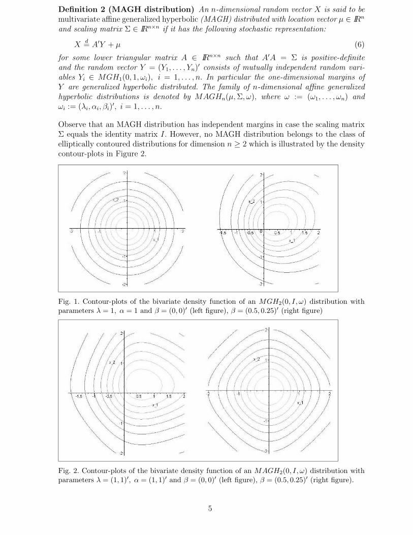
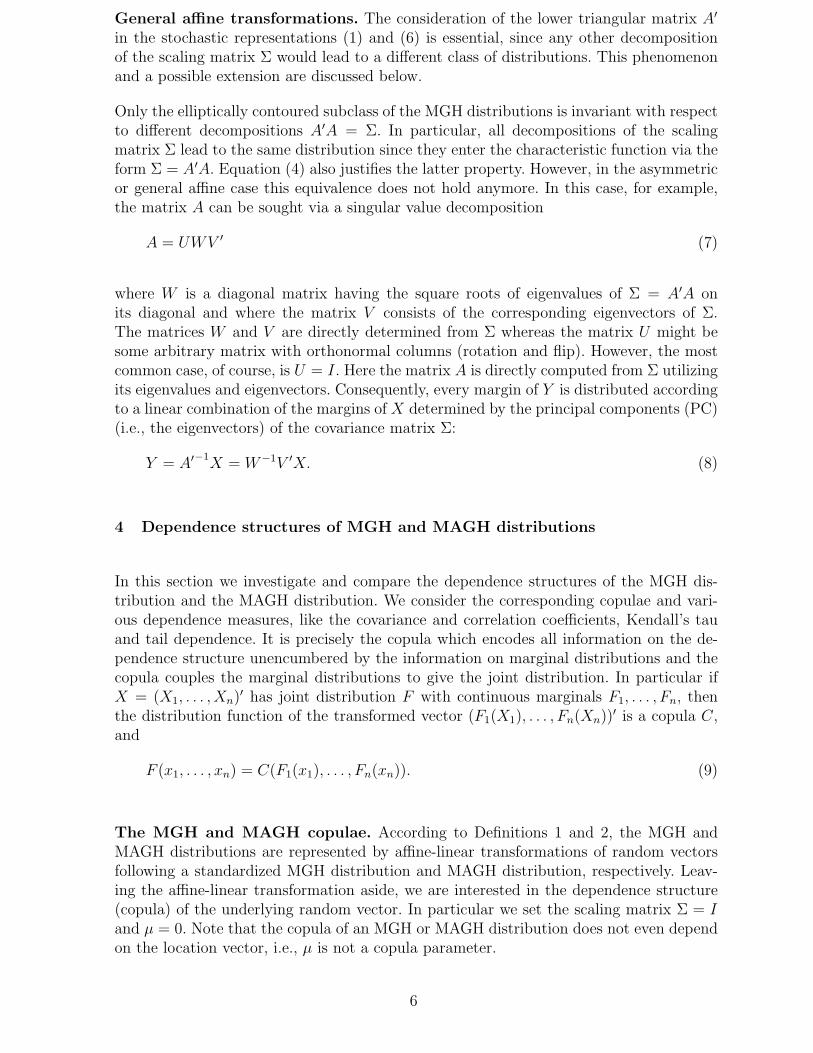
Observe that an MAGH distribution has independent margins in case the scaling matrixΣ equals the identity matrix I. However, no MAGH distribution belongs to the class ofelliptically contoured distributions for dimension n ≥ 2 which is illustrated by the densitycontour-plots in Figure 2.

Fig. 1. Contour-plots of the bivariate density function of an MGH2(0, I, ω) distribution withparameters λ = 1, α = 1 and β = (0, 0)′ (left figure), β = (0.5, 0.25)′ (right figure)

Fig. 2. Contour-plots of the bivariate density function of an MAGH2(0, I, ω) distribution withparameters λ = (1, 1)′, α = (1, 1)′ and β = (0, 0)′ (left figure), β = (0.5, 0.25)′ (right figure).

5

General affine transformations. The consideration of the lower triangular matrix A′

in the stochastic representations (1) and (6) is essential, since any other decompositionof the scaling matrix Σ would lead to a different class of distributions. This phenomenonand a possible extension are discussed below.

Only the elliptically contoured subclass of the MGH distributions is invariant with respectto different decompositions A′A = Σ. In particular, all decompositions of the scalingmatrix Σ lead to the same distribution since they enter the characteristic function via theform Σ = A′A. Equation (4) also justifies the latter property. However, in the asymmetricor general affine case this equivalence does not hold anymore. In this case, for example,the matrix A can be sought via a singular value decomposition

A = UWV ′ (7)

where W is a diagonal matrix having the square roots of eigenvalues of Σ = A′A onits diagonal and where the matrix V consists of the corresponding eigenvectors of Σ.The matrices W and V are directly determined from Σ whereas the matrix U might besome arbitrary matrix with orthonormal columns (rotation and flip). However, the mostcommon case, of course, is U = I. Here the matrix A is directly computed from Σ utilizingits eigenvalues and eigenvectors. Consequently, every margin of Y is distributed accordingto a linear combination of the margins of X determined by the principal components (PC)(i.e., the eigenvectors) of the covariance matrix Σ:

Y = A′−1X = W−1V ′X. (8)

4 Dependence structures of MGH and MAGH distributions

In this section we investigate and compare the dependence structures of the MGH dis-tribution and the MAGH distribution. We consider the corresponding copulae and vari-ous dependence measures, like the covariance and correlation coefficients, Kendall’s tauand tail dependence. It is precisely the copula which encodes all information on the de-pendence structure unencumbered by the information on marginal distributions and thecopula couples the marginal distributions to give the joint distribution. In particular ifX = (X1, . . . , Xn)′ has joint distribution F with continuous marginals F1, . . . , Fn, thenthe distribution function of the transformed vector (F1(X1), . . . , Fn(Xn))′ is a copula C,and

F (x1, . . . , xn) = C(F1(x1), . . . , Fn(xn)). (9)

The MGH and MAGH copulae. According to Definitions 1 and 2, the MGH andMAGH distributions are represented by affine-linear transformations of random vectorsfollowing a standardized MGH distribution and MAGH distribution, respectively. Leav-ing the affine-linear transformation aside, we are interested in the dependence structure(copula) of the underlying random vector. In particular we set the scaling matrix Σ = Iand µ = 0. Note that the copula of an MGH or MAGH distribution does not even dependon the location vector, i.e., µ is not a copula parameter.

6

Theorem 3 Let Y ∈MGHn(0, I, ω). Then the copula density function of Y is given by

c(u1, . . . , un)

= cKλ−n/2(α

√1 + y′y)

(1 + y′y)n/4−λ/2

n∏

i=1

(1 + y2i )

1/4−λ/2

Kλ−1/2(α√

1 + y2i )

exp(αβ′y)

exp(∏n

i=1 αβiyi)

∣

∣

∣

∣

∣

∣

yi=F−1i

(ui)

for ui ∈ [0, 1], i = 1, . . . , n, and some normalizing constant c. Here Fi refers to thedistribution function of the one-dimensional margin Yi, i = 1, . . . , n.

Let Y ∈MAGHn(0, I, ω). Then the corresponding copula equals the independence copula,i.e, the copula density function is given by

c(u1, . . . , un) ≡ 1, ui ∈ [0, 1], i = 1, . . . , n. (10)

Proof. Suppose Y ∈MGHn(0, I, ω). Then Y has a continuous and strictly positive densityfunction f. Utilizing formula (9) we obtain the copula density function by

c(u1, . . . , un) =f(y1, . . . , yn)∏n

i=1 fi(yi)

∣

∣

∣

∣

∣

yi=F−1i

(ui)

. (11)

Inserting the density function (2) into (11) yields the first assertion. Assume now thatY ∈ MAGHn(0, I, ω). Then Y has independent margins if and only if Y possesses theindependence copula C(u1, . . . , un) = u1 · . . . · un according to Theorem 2.10.14 in Nelsen(1999). 2

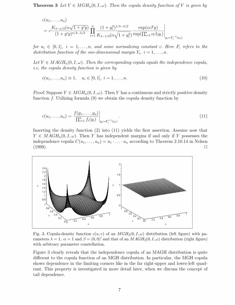
Fig. 3. Copula-density function c(u, v) of an MGH2(0, I, ω) distribution (left figure) with pa-rameters λ = 1, α = 1 and β = (0, 0)′ and that of an MAGH2(0, I, ω) distribution (right figure)with arbitrary parameter constellation.

Figure 3 clearly reveals that the independence copula of an MAGH distribution is quitedifferent to the copula function of an MGH distribution. In particular, the MGH copulashows dependence in the limiting corners like in the far right-upper and lower-left quad-rant. This property is investigated in more detail later, when we discuss the concept oftail dependence.

7

According to Theorem 2.10.12 in Nelsen (1999), any copula function is bounded frombelow (above) by the lower (upper) Frechet bound, i.e.,

W (u1, . . . , un) ≤ C(u1, . . . , un) ≤M(u1, . . . , un), (12)

where W (u1, . . . , un) = max(u1+ . . .+un−n+1, 0) and M(u1, . . . , un) = min(u1, . . . , un).Let Π(u1, . . . , un) = u1 · . . . · un be the product or independence copula. Note that M andΠ are always copula functions. However, W is only a copula for dimension n = 2.

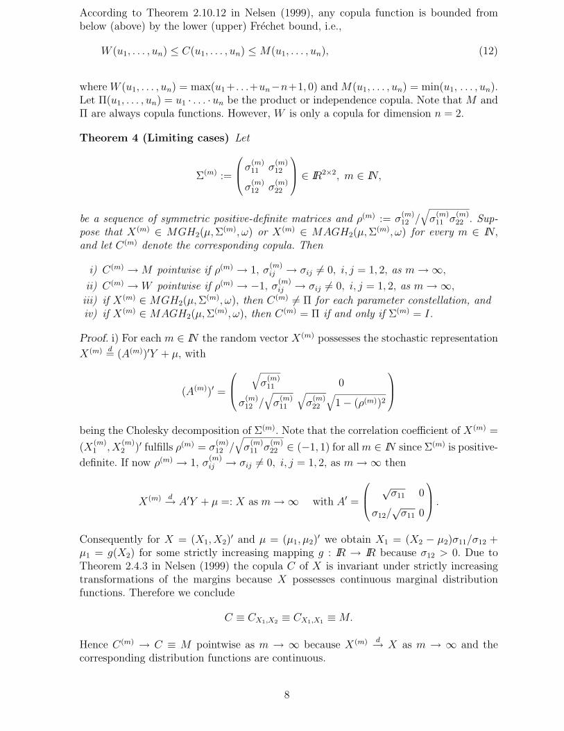
Theorem 4 (Limiting cases) Let

Σ(m) :=

σ(m)11 σ

(m)12

σ(m)12 σ

(m)22

∈ IR2×2, m ∈ IN,

be a sequence of symmetric positive-definite matrices and ρ(m) := σ(m)12 /

√

σ(m)11 σ

(m)22 . Sup-

pose that X(m) ∈ MGH2(µ,Σ(m), ω) or X(m) ∈ MAGH2(µ,Σ

(m), ω) for every m ∈ IN,and let C(m) denote the corresponding copula. Then

i) C(m) →M pointwise if ρ(m) → 1, σ(m)ij → σij 6= 0, i, j = 1, 2, as m→ ∞,

ii) C(m) → W pointwise if ρ(m) → −1, σ(m)ij → σij 6= 0, i, j = 1, 2, as m→ ∞,

iii) if X(m) ∈MGH2(µ,Σ(m), ω), then C(m) 6= Π for each parameter constellation, and

iv) if X(m) ∈MAGH2(µ,Σ(m), ω), then C(m) = Π if and only if Σ(m) = I.

Proof. i) For each m ∈ IN the random vector X(m) possesses the stochastic representation

X(m) d= (A(m))′Y + µ, with

(A(m))′ =

√

σ(m)11 0

σ(m)12 /

√

σ(m)11

√

σ(m)22

√

1 − (ρ(m))2

being the Cholesky decomposition of Σ(m). Note that the correlation coefficient of X(m) =

(X(m)1 , X

(m)2 )′ fulfills ρ(m) = σ

(m)12 /

√

σ(m)11 σ

(m)22 ∈ (−1, 1) for allm ∈ IN since Σ(m) is positive-

definite. If now ρ(m) → 1, σ(m)ij → σij 6= 0, i, j = 1, 2, as m→ ∞ then

X(m) d→ A′Y + µ =: X as m→ ∞ with A′ =

√σ11 0

σ12/√σ11 0

.

Consequently for X = (X1, X2)′ and µ = (µ1, µ2)

′ we obtain X1 = (X2 − µ2)σ11/σ12 +µ1 = g(X2) for some strictly increasing mapping g : IR → IR because σ12 > 0. Due toTheorem 2.4.3 in Nelsen (1999) the copula C of X is invariant under strictly increasingtransformations of the margins because X possesses continuous marginal distributionfunctions. Therefore we conclude

C ≡ CX1,X2≡ CX1,X1

≡M.

Hence C(m) → C ≡ M pointwise as m → ∞ because X(m) d→ X as m → ∞ and thecorresponding distribution functions are continuous.

8

ii) The second assertion can be shown analogously, using the fact that

C ≡ CX1,X2≡ CX1,g(−X1) ≡ CX1,−X1

≡ W

for some strictly increasing mapping g : IR → IR.

iii) Suppose X(m) ∈ MGH2(µ,Σ(m), ω). Then X(m) possesses the product copula if and

only if it has independent margins (see Theorem 2.4.2 in Nelsen (1999)). According toDefinition 1, X(m) does not have independent margins if Σ(m) is not a diagonal matrix.Thus it suffices to consider Σ(m) = I. Further we can put β = 0 since β has no influenceon the factorization of the density function of an MGH distribution (see formula (2)).However, in that case X(m) belongs to the family of elliptically contoured distributions.Therefore Theorem 4.11 in Fang, Kotz, and Ng (1990) implies that X(m) possesses inde-pendent margins if and only if X(m) is has a bivariate normal distribution. Since normaldistributions and MGH distributions are disjoint classes of distributions, the assertionfollows.

iv) According to Definition 2, MAGH distributions have independent margins if and onlyif Σ = I. 2

Remark. The results of Theorem 4 can be extended to n-dimensional MGH and MAGHdistributions. However, for n ≥ 3 the lower Frechet bound is not a copula function any-more; see Theorem 2.10.13 in Nelsen (1999) for an interpretation of the lower Frechetbound in that case.

The covariance and correlation matrix. Among the large number of dependence mea-sures for multivariate random vectors the covariance and the correlation matrix are stillthe most favorite ones in most practical applications. Many multivariate models in financeare based on these linear dependence measures which are appropriate under the assump-tion of a normal distribution. However, as we have already mentioned, several empiricalinvestigations reject the hypothesis of a multivariate normal distribution to be suited forfinancial data-modelling. Consequently, new distribution models like the present MGHand MAGH model have been introduced where dependence measures describing only lin-ear dependence between bivariate random vectors should be considered with care. Often,”scale-invariant” dependence measures like Kendall’s tau seem to be more appropriate;for more details we refer to Embrechts, McNeil, and Straumann (1999). According toLindskog, McNeil, and Schmock (2003), the correlation matrix represents a reasonabledependence measure within the class of elliptically contoured distributions.

Theorem 5 (Mean and covariance for MGH distributions)

Let X ∈ MGHn(µ,Σ, ω) and define Rλ,i(x) := Kλ+i(x)xiKλ(x)

. Then the mean vector and thecovariance matrix of X are given by

E[X] = µ+ αRλ,1

(√

α2(1 − β′β))

A′β

and

Cov[X] =Rλ,1

(√

α2(1 − β′β))

Σ

9

+[

Rλ,2

(√

α2(1 − β′β))

−R2λ,1

(√

α2(1 − β′β))

]

A′ββ′A

1 − β′β

For the symmetric case β = (0, . . . , 0)′ and λ = 1, the mean vector and the covariancematrix of X simplify to E[X] = 0 and Cov[X] = K2(α)/(αK1(α)) · Σ.

Proof. Let X ∈ MGHn(µ, Σ, ω) with parameter representation as in (5). Then X isdistributed according to a variance-mean mixture of a multivariate normal distribution,i.e., X|(Z = z) ∼ N(µ + zΣβ, zΣ), where the mixing random variable Z is distributed

according to a generalized inverse Gaussian distribution GIG(λ, δ,√

δ2(α2 − β′Σβ)) (seee.g. Barndorff-Nielsen, Kent, and Sørensen (1982)). Hence,

E[X] = µ+ ΣβEGIG[Z]

andE[XX ′] = µµ′ + (Σ + µβ′Σ + Σβµ′)EGIG[Z] + Σββ′ΣEGIG[Z2].

Therefore, the covariance matrix of X is given by

Cov[X] = ΣEGIG[Z] + Σββ′ΣV arGIG[Z].

According to Eberlein and Prause (1999), mean and variance of the mixing random vari-

able Z ∼ GIG(λ, δ,√

δ2(α2 − β′Σβ)) are given by

EGIG[Z] = Rλ,1(√

δ2(α2 − β′Σβ))

andV arGIG[Z] = δ4 · [Rλ,2(

√

δ2(α2 − β′Σβ)) −R2λ,1(

√

δ2(α2 − β′Σβ))].

Utilizing the parameter mapping δ2(α2 − β′Σβ) = α2(1 − β′β), Σβδ2 = ΣαA−1β andδ4Σββ′Σ = A′ββ′A yields the assertion. 2

Theorem 6 (Mean and covariance for MAGH distributions)Let X ∈MAGHn(µ,Σ, ω). Then the mean vector and the covariance matrix are given by

E[X] = A′eY + µ and Cov[X] = A′CA,

respectively, where eY = (E[Y1], . . . , E[Yn])′ with E[Yi] = Rλi,1(√

α2i (1 − β2

i ))αiβi andC = diag(c11, . . . , cnn) with

cii = Rλi,1(√

α2i (1 − β2

i )) + [Rλi,2(√

α2i (1 − β2

i )) −R2λi,1

(√

α2i (1 − β2

i ))]β2

i

1 − β2i

.

The covariance matrix Cov[X] is proportional to Σ if α = αi, β = βi and λ = λi for alli = 1, . . . , n.

Proof. The assertion follows immediately from Theorem 5 and equation (6). 2

Kendall’s tau. The correlation coefficient is a measure of linear dependence between tworandom variables and therefore it is not invariant under monotone increasing transforma-tions. However, not only does ”scale-invariance” present an undisputable requirement for

10

a proper dependence measure in general (cf. Joe (1997), Chapter 5), but also in practice”scale-invariant” dependence measures play an increasing role in dependence modelling.Kendall’s tau is the most famous one and therefore we determine it for MGH and MAGHdistributions.

Definition 7 (Kendall’s tau) Let X = (X1, X2)′ and X = (X1, X2)

′ be independentbivariate random vectors with common continuous distribution function F and copula C.Kendall’s tau is defined by

τ = IP((X1 − X1)(X2 − X2) > 0) − IP((X1 − X1)(X2 − X2) < 0)

= 4∫

[0,1]2

C(u, v) dC(u, v) − 1. (13)

Theorem 8 Let ρ ∈ (−1, 1) be the correlation coefficient of X1 and X2.

i) If X ∈MGH2(µ,Σ, ω) with β = 0, then

τ =2

πarcsin(ρ). (14)

ii) If X ∈ MAGH2(µ,Σ, ω) with stochastic representation Xd= A′Y + µ, A′A = Σ, then

for ρ 6= 0

τ =4

|c|∫

IR2

fY1(x1)

(

x2 − x1

c

)

·x1∫

−∞FY2

(

x2 − z

c

)

fY1(z) dzd(x1, x2) − 1, (15)

where c := sgn(ρ)√

1/ρ2 − 1. Further τ = 0 for ρ = 0.

The proof is given in the Appendix.

Remark. A closed form expression of Kendall’s tau for MAGH distributions (given by(15)) cannot be expected. However, since the density functions of Y1 and Y2 are explicitlygiven, formula (15) yields a tractable numerical solution.

Tail dependence. A strong emphasis in this paper is put on the dependence structureof MGH and MAGH distributions. In this context we establish the following result aboutthe dependence structure of extreme events (tail dependence or extremal dependence)related to the latter types of distributions. The importance of tail dependent especiallyin financial risk management is emphasized in Hauksson, Dacorogna, Domenig, Mueller,and Samorodnitsky (2001) and Embrechts, Lindskog, and McNeil (2003). The followingdefinition (according to Joe (1997), p. 33) represents one of many possible definitions oftail dependence.

Definition 9 (Tail dependence) Let X = (X1, X2)′ be a 2-dimensional random vector.

We say that X is upper tail-dependent if

λU := limu→1−

IP(X1 > F−11 (u) | X2 > F−1

2 (u)) > 0, (16)

11

where the limit is assumed to exist and F−11 , F−1

2 denote the generalized inverse dis-tribution functions of X1, X2, respectively. Consequently, we say that X is upper tail-independent if λU equals 0. Similarly, X is said to be lower tail-dependent (lower tail-independent) if λL > 0 (λL = 0), where λL := limu→0+ IP(X1 ≤ F−1

1 (u) | X2 ≤ F−12 (u)) if

existent.

Figure 3 reveals that bivariate standardized MGH distributions show more evidence ofdependence in the upper-right and lower-left quadrant of its distribution function thanMAGH distributions. However, the following theorem shows that MGH distributions arealways tail independent whereas non-standardized MAGH distributions can even modeltail dependence. For the sake of simplicity we restrict ourselves to the symmetric caseβ = 0.

Theorem 10 Let ρ ∈ (−1, 1) be the correlation coefficient of the bivariate distributionsconsidered below. Suppose β = 0. Theni) the MGH2(µ,Σ, ω) distributions are upper and lower tail-independent,ii) the MAGH2(µ,Σ, ω) distributions are upper and lower tail-independent if

α2 < α1

√

1/ρ2 − 1 or ρ ≤ 0, and

iii) the MAGH2(µ,Σ, ω) distributions are upper and lower tail-dependent if

α2 > α1

√

1/ρ2 − 1 and ρ > 0.

The proof is given in the Appendix.

Remark. Additionally to Theorem 10 it can be shown that an MGH2(µ,Σ, ω) distribu-

tion (with β = 0) is tail independent if α2 = α1

√

1/ρ2 − 1 and λ2 < λ1.

5 MGH versus MAGH: Advantages and disadvantages

In this section we list and compare some advantages and disadvantages of MGH distri-butions and MAGH distributions. We start with the distributional flexibility to fit realdata. An outstanding property of MAGH distributions is that, after an affine-linear trans-formation, all one-dimensional margins can be fitted separately via different generalizedhyperbolic distributions. In contrast to this, the one-dimensional margins of MGH distri-butions are not that flexible since the parameters α and λ relate to the entire multivariatedistribution and determine the strong structural behavior (see Definition 1). However,this structure causes a large subclass of MGH distributions to belong to the family ofelliptically contoured distributions which inherit many useful statistical and analyticalproperties from multivariate normal distributions.

Regarding the dependence structure, the MAGH distributions may have independent mar-gins for any parameter constellations ω = (ω1, . . . , ωn) (see Theorem 4). In particular,they also support models which are based on a linear combination of independent factors.In contrast, the MGH distributions are not capable of modelling independent margins.They even yield ”extremal” dependencies for bivariate distributions having correlationzero. Moreover, the correlation matrix of MAGH distributions is proportional to the scal-ing matrix Σ within a large subclass of asymmetric MAGH distributions (see Theorem6), whereas Σ is hardly to interpret for skewed MGH distributions. Further, the copula

12

of MAGH distributions, being the dependence structure of an affine-linear transformedrandom vector with independent components, is quite illustrative and possesses manyappealing modelling properties. On the other hand, the copula structure of MGH distri-butions may suffers from inflexibility. Regarding the dependence of extreme events, theMAGH distributions can model tail dependence whereas MGH distributions are alwaystail independent. Therefore, MAGH distributions are suitable especially within the fieldof risk management.

Sections 6 and 8 reveal that in contrast to MGH distributions, parameter estimation forMAGH distributions is considerably simpler and more robust. Even in an asymmetricenvironment, the parameters of MAGH distributions can be identified in a two stageprocedure which has a considerable computational advantage in higher dimensions. Thesame procedure can be applied for elliptically contoured MGH distributions (β = 0). Therandom vector generation algorithms for MGH and MAGH distributions turn out to beequally efficient and fast, irrespective of the dimension.

The simulations in Section 8 show that both distributions fit simulated and real datawell. Thus, summarizing the above advantages and disadvantages, the MAGH distribu-tions have much to recommend them regarding their parameter estimation, dependencestructure, and random vector generation. However, it depends also on the kind of appli-cation and the user’s taste which model to prefer.

6 Parameter estimation

6.1 MGH distributions

Minimizing the cross entropy. A general method to measure the similarity betweentwo distribution or density functions f ∗ and f, respectively, is given by the Kullbackentropy (see Kullback (1959)) which is defined as

HK(f, f∗) :=∫

IRn

f ∗(x) logf ∗(x)

f(x)dx (17)

=∫

IRn

f ∗(x) log f ∗(x)dx−∫

IRn

f ∗(x) log f(x)dx. (18)

The Kullback entropy is always nonnegative and is zero if the densities f and f ∗ areidentical. In our context, this relationship is useful to measure the similarity between the”true” density f ∗ and its approximation f . Therefore, minimizing the Kullback entropyby varying f is one way to find a good approximation of the ”true” density f ∗. Note thatthe first term in (17) is constant and can be dropped. This leads to the so-called crossentropy given by

H(f, f∗) := −∫

IRn

f ∗(x) log f(x)dx. (19)

13

Obviously the integral in (19) cannot be evaluated without knowledge of f ∗. Hence, thecorresponding distribution is approximated by its empirical counterpart, i.e., by the em-pirical distribution function

F ∗e (x) =

1

m

m∑

k=1

1Xk≤x, (20)

where Xk, k = 1, . . . ,m, denotes a random sample with distribution function F ∗. It iswell known that this procedure leads to an unbiased estimator of F ∗(x) (see, for example,Parzen (1962)).

An approximation of the integral in (19) is now given by

H(f, f∗) ≈ −∫

IRn

log f(x)dF ∗e (x) = − 1

m

m∑

k=1

log f(Xk). (21)

Thus, minimizing the cross entropy is approximately equivalent to maximizing the log-likelihood function.

For computational reasons it may be advantageous to work with the standardized vectory = B(x − µ) where B := A′−1. The density transformation theorem yields that the

density function fX of Xd= A′Y + µ ∈MGH(µ,Σ, ω) is given by

fX(x) = fA′Y +µ(x) = |B|fY (y), (22)

with |B| > 0 being the determinant of B. The following expression indicates the parame-terization of the negative log-likelihood function L while utilizing the above standardiza-tion:

L(X, η) = −m

∑

k=1

log(|B|) −m

∑

k=1

log(fY (ω,B(Xk − µ))) (23)

with parameters η = (µ,B, ω) and ω = (λ, α, β).

While the location vector µ can take arbitrary values in IRn, B and ω are subject tovarious constraints. The matrix B must be triangular with positive diagonal such thatA′A is positive-definite. The parameter α is supposed to be positive and the vector βmust fulfill ||β||2 ≤ 1.

Many approaches are possible regarding the latter optimization problem, inter alia wemention two methods:

• constrained nonlinear optimization methods, and• unconstrained nonlinear optimization methods after suitable parameter transforma-

tions.

We prefer the unconstrained approach due to robustness and efficiency reasons. The fol-lowing parameter transformations are appropriate.

14

The matrix B can be sought of the form B = UD where D is some diagonal matrix havingstrictly positive elements and U is a triangular matrix having only ones on its diagonal.In order to enforce the strict positivity of the diagonal elements dii, i = 1, . . . , n, of D, thefollowing transformations are applied:

bii = dii = eνi , i = 1, . . . , n,

bij = diiuij = eνiuij, i = 1, . . . , n− 1; j = 2, . . . , n; j > i

with unknown parameters νi and uij. The parameter α is estimated via the same expo-nential map. For the vector β we utilize the smooth transformation

β = γ1

1 + exp(−‖γ‖2)· 1

‖γ‖2

. (24)

After the transformations we are now confronted with the new optimization problem

minη∈Ω

L(X, η)

where Ω = IR(3+(n−1)/2)n+2 and η denotes the transformed unconstrained parameters. Sincein general the objective function is non-convex, a global numerical optimization methodis required. Optimization methods can be subdivided into deterministic and probabilisticmethods. As far as deterministic methods are concerned, certain assumptions on theobjective function have to be imposed (like Lipschitz conditions) in order to guarantee atermination of the optimization routine in finitely many steps. Probabilistic methods, incontrast, have better convergence properties but only with a certain likelihood. Here theassumptions on the objective function are rather weak.

The algorithm we use belongs to the probabilistic ones and consists of two characteristicphases:

1. In a global phase the objective function is evaluated at a random number of points beingpart of the search space.

2. In a local phase the samples are transformed to become candidates for local optimizationroutines.

Thus, the global phase is responsible for the convergence result of the optimization routinewhile the local phase determines the efficiency of the optimization. In the ideal (but hardlyattainable) case, only a few local optimizations are necessary as there are attractors in therange of the objective function (e.g. regions where the minimum is reached by gradientdescent). We mentioned already that the probabilistic algorithms find a global solutiononly with a given probability. Rinnooy Kan and Timmer (1987) show the convergence ofprobabilistic algorithms to the global minimum under certain conditions. This motivates ausage of the Multi-Level Single-Linkage procedure (see Rinnooy Kan and Timmer (1987)).Here the global optimization method generates random samples from the search space byidentifying the samples belonging to the same objective function attractor and eliminatingmultiple ones. For the remaining samples in the local phase a conjugate gradient method(see Fletcher (1987)) is started. Further, a Bayesian stopping rule is applied in orderto assess the probability that all attractors have been explored. For an account on theBayesian stopping rule we refer the reader to Boender and Rinnooy Kan (1987).

15

6.2 MAGH distributions

The parameters of the MAGH distribution function can be easily identified in a two-stageprocedure comprising the following steps:

(1) Compute the sample covariance matrix S of the random vector X. Transforme Xto the vector Y = BX with independent margins. The matrix B is received viaCholesky decomposition S−1 = B′B.

(2) Identify the parameters λi, αi and βi which belong to the univariate marginal dis-tributions of Y. The location vector µ can be received via B−1e with ei being thelocation parameter of Yi (see Theorem 5). The scaling matrix Σ equals B−1′DB−1

where the diagonal matrix D is determined by the scaling parameters of Yi on itsdiagonal.

The latter procedure simplifies the complexity of the numerical optimization a lot.

Note that the parameters of MAGH distributions can be estimated analogously to theprocedure described for MGH distributions. However, instead of the multivariate density(2), a product of n univariate densities

f1(y) = cKλ−1/2(α

√1 + y2)

(1 + y2)1/4−λ/2eαβy (25)

with normalizing constant

c =α1/2 (1 − β2)

λ/2

(2π)1/2Kλ(α√

1 − β2)(26)

is considered. It is important for applications that the univariate densities are not necessar-ily identically parameterized. This means that the margins may have different parametersλi, αi, βi, i = 1, . . . , n. In other words, there is a considerable freedom of choosing theparameters λ, α and β. Therefore, in addition to a parameterization similar to that forMGH distributions (i.e., the same λ and α for all one-dimensional margins and differentβi) two further extreme alternatives are possible:

• Minimum parameterization: Equal parameters λ, α and β for all one-dimensional mar-gins.

• Maximum parameterization: Individual parameters λi, αi and βi for all one-dimensionalmargins.

The appropriate parameterization depends on the kind of application and the availabledata volume.

The optimization procedure presented in this section is a special case of an identifica-tion-algorithm for conditional distributions explored in Stutzle and Hrycej (2001, 2002a,2002b).

16

7 Sampling from MGH and MAGH distributions

Additionally to the estimation procedures described in Section 6, in this section we providean efficient and self-contained random vector generation for the families of MGH andMAGH distributions. Fast sampling from an MGHn(µ,Σ, ω) distribution is possible viathe following variance-mean mixture representation.

Let the random variable Z be distributed according to a generalized inverse Gaussiandistribution with parameters λ, χ and ψ. In particular the latter family is referred to as theGIG(λ, χ, ψ) distributions. Then,X ∈MGHn(µ,Σ, ω) is conditionally normal distributedwith mixing random variable Z, i.e., X|(Z = z) ∼ Nn(µ + zβ, z∆), where ∆ ∈ IRn×n isa symmetric positive-definite matrix with determinant |∆| = 1 and µ, β ∈ IRn. Theparameters Σ and ω = (λ, α, β) are given by

α =√

(ψ + β′∆β)χ, β = 1/√

ψ + β′∆βLβ, Σ = χ · ∆

with Cholesky decomposition L′L = ∆. The inverse map is given by

χ = |Σ|1/n, ψ = α2/|Σ|1/n · (1 − β′β), ∆ = Σ/|Σ|1/n, and β = α · (A)−1β

with Cholesky decomposition A′A = Σ.

The sampling algorithm is now of the following form: A pseudo random number is sampledfrom a random variable Z having a generalized inverse Gaussian distribution with param-eters λ, χ, and ψ. Then an n-dimensional random vector X being conditionally normaldistributed with mean vector µ+Z∆β (”drift”) and covariance matrix Z∆ (determinant|∆| = 1) is generated.

The density function of the generalized inverse Gaussian distribution GIG(λ, χ, ψ), isgiven by

fZ(x) = c · xλ−1 exp(

− χ

2x− ψx

2

)

, x > 0, (27)

with normalizing constant c = (ψ/χ)λ/2/(2Kλ(√ψχ)). The range of the parameters is

given by

i) χ > 0, ψ ≥ 0 if λ < 0, orii) χ > 0, ψ > 0 if λ = 0, oriii) χ ≥ 0, ψ > 0 if λ > 0.

The following efficient algorithm is formulated for multivariate generalized hyperbolicdistributions MGHn(µ,Σ, ω) with parameter λ = 1. Section 8.1 justifies the restriction tothat class of distributions. In this context the GIG(λ, χ, ψ) distribution is referred to asinverse Gaussian distribution. However, the algorithm can be easily extended to general λ.Our empirical study shows that the algorithm outperforms the efficiency of the samplingalgorithm proposed by Atkinson (1982) which suites to a larger class of distributions (seealso Prause (1999), Section 4.6). Moreover, the algorithm avoids tedious minimizationroutines and time-consuming evaluations of the Bessel functionKλ. The generation utilizes

17

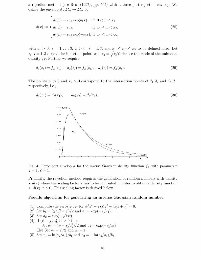
a rejection method (see Ross (1997), pp. 565) with a three part rejection-envelop. Wedefine the envelop d : IR+ → IR+ by

d(x) :=

d1(x) = ca1 exp(b1x), if 0 < x < x1,

d2(x) = ca2, if x1 ≤ x < x2,

d3(x) = ca3 exp(−b3x), if x2 ≤ x <∞,

(28)

with ai > 0, i = 1, . . . , 3, bi > 0, i = 1, 3, and x1 ≤ x2 ≤ x3 to be defined later. Let

zi, i = 1, 3 denote the inflection points and z2 =√

χ/ψ denote the mode of the unimodaldensity fZ . Further we require

d1(z1) = fZ(z1), d2(z2) = fZ(z2), d3(z3) = fZ(z3). (29)

The points x1 > 0 and x2 > 0 correspond to the intersection points of d1, d2 and d2, d3,respectively, i.e.,

d1(x1) = d2(x1), d2(x2) = d3(x2). (30)

Fig. 4. Three part envelop d for the inverse Gaussian density function fZ with parametersχ = 1 , ψ = 1.

Primarily, the rejection method requires the generation of random numbers with densitys ·d(x) where the scaling factor s has to be computed in order to obtain a density functions · d(x), x > 0. This scaling factor is derived below.

Pseudo algorithm for generating an inverse Gaussian random number:

(1) Compute the zeros z1, z2 for ψ2z4 − 2χψz2 − 4χz + χ2 = 0.(2) Set b1 = (χ/z2

1 − ψ)/2 and a1 = exp(−χ/z1).(3) Set a2 = exp(−

√χψ).

(4) If (ψ − χ/z22)/2 > 0 then

Set b3 = (ψ − χ/z22)/2 and a3 = exp(−χ/z2)

Else Set b3 = ψ/2 and a3 = 1.(5) Set x1 = ln(a2/a1)/b1 and x2 = − ln(a2/a3)/b3.

18

(6) Set

s =(a1

b1exp(b1x1) −

a1

b1+ (x2 − x1)a2 +

a3

b3exp(−b3x2)

)

.

(7) Set

k1 =1

s

(a1

b1exp(b1x1) −

a1

b1

)

and k2 = k1 +1

s(x2 − x1)a2.

(8) Generate independent and uniformly distributed random numbers U and V on theinterval [0, 1].

(9) If U ≤ k1 goto step 10.ElseIf k1 < U ≤ k2 goto step 11.Else goto step 12.

(10) Set

x =1

b1ln(

b1a1

sU + 1).

If

V ≤ fZ(x)

d1(x)=

1

a1

exp(

− (χx−1 + ψx

2+ b1x)

)

Then Return xElse goto step 8.

(11) Set

x =sU

a2

− a1

b1a2

(

exp(b1x1) − 1)

+ x1.

If

V ≤ fZ(x)

d2(x)=

1

a2

exp(

− (χx−1 + ψx

2))

Then Return xElse goto step 8.

(12) Set

x = − 1

b3ln

[

− b3a3

sU − a1

b1(eb1x1 − 1) − (x2 − x1)a2 −

a3

b3e−b3x2

]

.

If

V ≤ fZ(x)

d3(x)=

1

a3

exp(

− (χx−1 + ψx

2) + b3x

)

Then Return xElse goto step 8.

Remark. In order to generate a sequence of inverse Gaussian random numbers repeatstep 8.

So far we have generated random numbers from an univariate inverse Gaussian distri-bution. We turn now to the generation of multivariate generalized hyperbolic randomvectors. For this we exploit the above introduced mixture representation.

Pseudo algorithm for generating an MGH vector:

(1) Set ∆ = L′L via Cholesky decomposition.(2) Generate an inverse Gaussian random number Z with parameters χ and ψ.(3) Generate a standard normal random vector N.

19

(4) Return X = µ+ Z∆β +√ZL′N.

Pseudo algorithm for generating an MAGH vector:

(1) Set Σ = A′A via Cholesky decomposition.(2) Generate a random vector Y with independent MGH1(0, 1, ωi), i = 1, . . . , n, dis-

tributed components (see above).(3) Return X = µ+ A′Y.

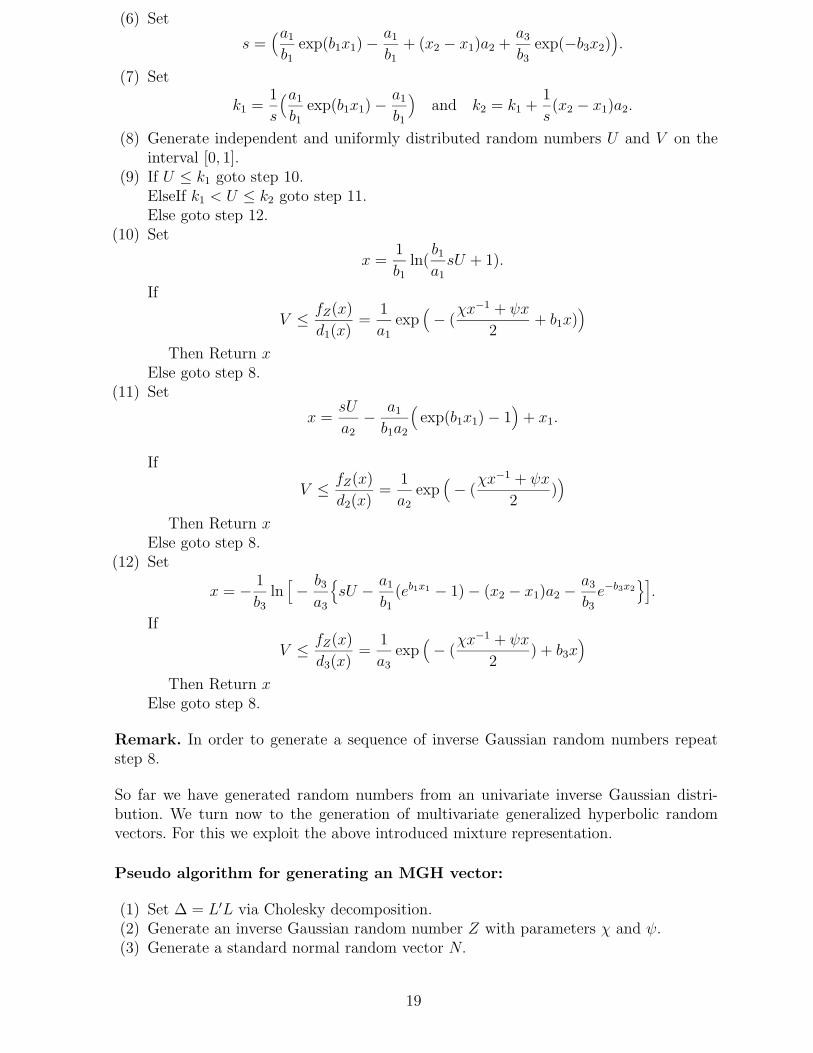
Table 1 presents values of empirical efficiency of the MGH random vector generator forvarious parameter constellations. In our framework, efficiency is defined by the followingratio

Efficiency =] of generated samples

] of algorithm-passes including rejections.

χ/ψ 0.1 0.5 1 2 5 10

0.1 0.94 0.913 0.904 0.886 0.877 0.872

0.5 0.916 0.884 0.877 0.865 0.859 0.852

1 0.901 0.877 0.867 0.863 0.857 0.851

2 0.889 0.866 0.857 0.856 0.856 0.845

5 0.876 0.858 0.854 0.852 0.847 0.849

10 0.866 0.86 0.851 0.853 0.842 0.847

Table 1Empirical efficiency of the MGH random number generator for λ = 1 and 10, 000 generatedsamples.

8 Simulation and empirical study

A series of computational experiments with simulated data is performed in this section.The experiments disclose that

• MGH density functions with arbitrary parameter λ seem to have very close counterpartsin the MGH-subclass with λ = 1,

• The MAGH model can closely approximate the MGH model with similar parametervalues.

8.1 Arbitrary MGH distributions versus MGH distributions with parameter λ = 1 (MH)

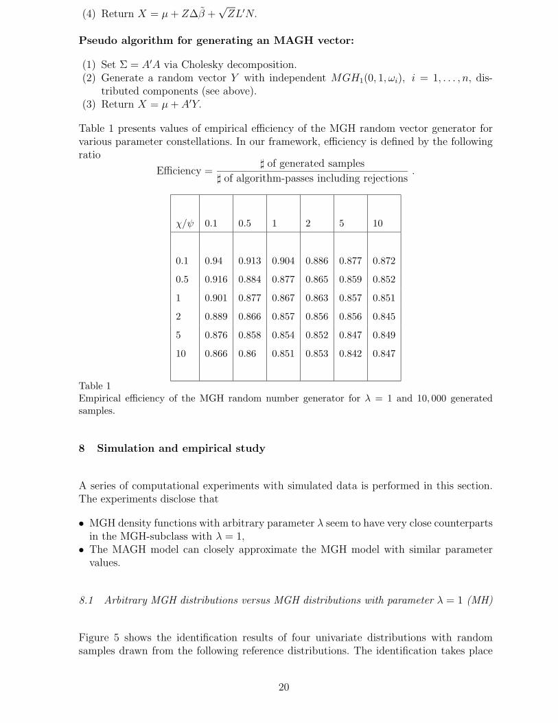
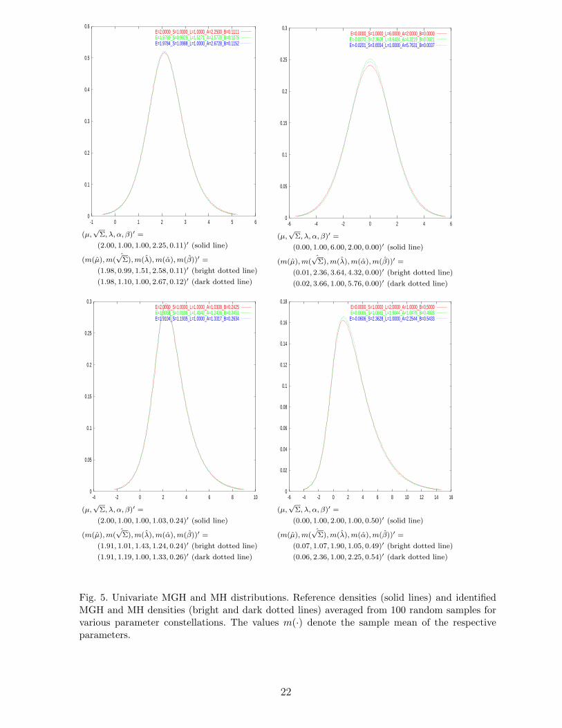
Figure 5 shows the identification results of four univariate distributions with randomsamples drawn from the following reference distributions. The identification takes place

20

either under the assumption of an arbitrary generalized hyperbolic distribution or ofa generalized hyperbolic distribution with fixed λ = 1 (in short: MH distribution). Inboth pictures on the left half of the figure, samples were drawn from the generalizedhyperbolic distribution with fixed parameter λ = 1. They illustrate the phenomenonthat although the identification procedure for MGH densities frequently produces λ 6= 1,the approximation of the density function remains good. The pictures on the right sideillustrate the opposite case, namely, a good approximation of the MGH density function(λ 6= 1) via the MH density function (λ = 1).

Consider now an MGH2(µ,Σ, ω) distribution with Σ =

σ11 σ12

σ12 σ22

. The mutual tradeoff

between λ, α and the scaling parameters S1 :=√σ11 and S2 :=

√σ22 for the latter

distribution function is shown in Table 2. While all samples were drawn from an MHdistribution, MGH identifications usually lead to an overestimate of λ which is traded offby lower values of α, S1 and S2. In contrast to that, the parameter identifications for MHdistributions are close to the reference values. However, the differences between the crossentropies are hardly discernible, showing that both parameter combinations correspondto densities which are close to each other.

The following conclusions can be drawn:

• The fit of both distributions, MGH and MH distribution, measured by cross entropy andvisual closeness of the plots, is satisfying. This implies the existence of multiple param-eter constellations for MGH distribution functions which lead to quite similar densityfunctions. Similar results have been observed for the corresponding tail functions.

• Generalized hyperbolic densities seem to have very close counterparts in the class ofMH distributions (even for large λ). Therefore, the class of MH distributions will besufficiently rich for our considerations.

In view of the above results, only MH distributions and the corresponding MAH dis-tributions (multivariate affine generalized hyperbolic distributions with λ = 1) will beconsidered in the next section.

8.2 MH distributions versus MAH distributions

The estimation of parameters is compared for the following three classes of bivariatedistributions:

(1) MH distributions.(2) MAH distributions with minimal parameter configuration (same value of α and β for

each margin).(3) MAH distributions with maximal parameter configuration (different values of αi and

βi for each margin).

All types of distributions in Table 3 have been identified from data which were sampledfrom an MH distribution. The two stage algorithm introduced in Section 6.2 has been usedfor the identification of the MAHmax model (determining first the sample correlation ma-

21

0

0.05

0.1

0.15

0.2

0.25

0.3

-4 -2 0 2 4 6 8 10

E=2.0000_S=1.0000_L=1.0000_A=1.0308_B=0.2425E=1.9058_S=1.0108_L=1.4342_A=1.2406_B=0.2451E=1.9104_S=1.1935_L=1.0000_A=1.3317_B=0.2634

(1.91, 1.19, 1.00, 1.33, 0.26)′ (dark dotted line)

(1.91, 1.01, 1.43, 1.24, 0.24)′ (bright dotted line)

(m(µ), m(√

Σ), m(λ), m(α), m(β))′ =

(2.00, 1.00, 1.00, 1.03, 0.24)′ (solid line)

(µ,√

Σ, λ, α, β)′ =

0

0.1

0.2

0.3

0.4

0.5

0.6

-1 0 1 2 3 4 5 6

E=2.0000_S=1.0000_L=1.0000_A=2.2500_B=0.1111E=1.9789_S=0.9929_L=1.5171_A=2.5770_B=0.1079E=1.9784_S=1.0988_L=1.0000_A=2.6728_B=0.1152

(1.98, 1.10, 1.00, 2.67, 0.12)′ (dark dotted line)

(1.98, 0.99, 1.51, 2.58, 0.11)′ (bright dotted line)

(m(µ), m(√

Σ), m(λ), m(α), m(β))′ =

(2.00, 1.00, 1.00, 2.25, 0.11)′ (solid line)

(µ,√

Σ, λ, α, β)′ =

0

0.02

0.04

0.06

0.08

0.1

0.12

0.14

0.16

0.18

-6 -4 -2 0 2 4 6 8 10 12 14 16

E=0.0000_S=1.0000_L=2.0000_A=1.0000_B=0.5000E=0.0686_S=1.0665_L=1.9044_A=1.0478_B=0.4928

E=-0.0606_S=2.3628_L=1.0000_A=2.2544_B=0.5433

(0.06, 2.36, 1.00, 2.25, 0.54)′ (dark dotted line)

(0.07, 1.07, 1.90, 1.05, 0.49)′ (bright dotted line)

(m(µ), m(√

Σ), m(λ), m(α), m(β))′ =

(0.00, 1.00, 2.00, 1.00, 0.50)′ (solid line)

(µ,√

Σ, λ, α, β)′ =

0

0.05

0.1

0.15

0.2

0.25

0.3

-6 -4 -2 0 2 4 6

E=0.0000_S=1.0000_L=6.0000_A=2.0000_B=0.0000E=-0.0070_S=2.3608_L=3.6424_A=4.3219_B=0.0021E=-0.0201_S=3.6554_L=1.0000_A=5.7631_B=0.0037

(0.02, 3.66, 1.00, 5.76, 0.00)′ (dark dotted line)

(0.01, 2.36, 3.64, 4.32, 0.00)′ (bright dotted line)

(m(µ), m(√

Σ), m(λ), m(α), m(β))′ =

(0.00, 1.00, 6.00, 2.00, 0.00)′ (solid line)

(µ,√

Σ, λ, α, β)′ =

Fig. 5. Univariate MGH and MH distributions. Reference densities (solid lines) and identifiedMGH and MH densities (bright and dark dotted lines) averaged from 100 random samples forvarious parameter constellations. The values m(·) denote the sample mean of the respectiveparameters.

22

trix, then transforming the variables, and finally identifying the univariate distributions).The identification results are provided in Table 3.

The following conclusions can be drawn:

• For all three models, most parameters show an acceptable fit regarding the sample biasand the sample standard deviation. The relative variability of the estimates increaseswith decreasing α (fatter tailed distributions). Such fatter tailed distributions seem tobe more ill-posed with respect to the estimation of individual parameters.

• The differences between the parameter estimates obtained either for the MH, the MAH-min, or the MAHmax distribution are negligible (although the data are drawn from anMH distribution).

• The fit in terms of the cross entropy does not differ significantly between the variousmodels. As expected, the MAHmax estimates are closer to the MH reference distributionthan the MAHmin estimates are in terms of the cross entropy (Note that in one case theyare even better than the MH estimates). The fitting capability of the MAHmax modelcomes at the expense of a larger variability and sometimes larger bias (”overlearningeffect”).

9 Application to financial data

The MGH and MAGH distributions have been fitted to various asset-return data. Inparticular, the following distributions have been used:

(1) MGH/MH,(2) MAGH/MAH with minimum parameterization (denoted by (min)), that is, with all

margins equally parameterized,(3) MAGH/MAH with maximum parameterization (denoted by (max)), that is, with

each margin individually parameterized.

For some of these distributions we have also estimated the symmetric pendant (denoted by(sym)), i.e., β = 0. Further, we illustrate estimations following the affine transformationmethod provided at the end of Section 3 (denoted by (PC)).

The results are presented in Table 4. The dependence parameter Dep.Par. refers to thesub-diagonal elements of the normed matrix Σ, i.e., Dep.Par.:= σij/

√σiiσjj = σij/(SiSj).

The maximum parameterized MAGH distribution frequently reach the best fit in termsof the cross entropy. Considerable variations between λ and α among the various modelscan be observed. This may lead to a similar variation of the scaling parameters whichfrequently behave contrary to the variation of the shape parameters.

Due to the total or approximate symmetry of some distribution models, the dependenceparameters can be roughly interpreted as ”correlation coefficients” for MGH and MAGH-min distributions. They are even close to the corresponding sample correlation coefficient(column ”Corr.”). Note that such an interpretation is not possible for the MAGHmaxmodel, due to the different parameterization of the one-dimensional margins.

23

Conclusion

Summarizing the results we have investigated an interesting new class of multidimen-sional distributions with exponentially decreasing tails to analyze high-dimensional data,namely the multivariate affine generalized hyperbolic distributions. These distributionsare attractive regarding the estimation of unknown parameters and random vector gen-eration. We illustrated that this class of distributions possesses an appealing dependencestructure and we derived several dependence properties. Finally, an extensive simulationstudy showed the flexibility and robustness of the introduced model. Thus, the usage ofmultivariate affine generalized hyperbolic distributions is recommended for multidimen-sional data modelling in statistical and financial applications.

Appendix

Proof (Theorem 8). i) Suppose X ∈ MGH2(µ,Σ, ω) with parameter β = 0. Then Xbelongs to the family of elliptically contoured distributions and the assertion follows byTheorem 2 in Lindskog, McNeil, and Schmock (2003).

ii) Suppose X ∈MAGH2(µ,Σ, ω) with stochastic representation Xd= A′Y +µ, A′A = Σ

and copula C. In particular

Σ =

σ11 σ12

σ12 σ22

and A′ =

√σ11 0

σ12/√σ11

√σ22

√1 − ρ2

with ρ being the correlation coefficient of X1 and X2. For ρ = 0, the assertion follows byTheorem 5.1.9 in Nelsen (1999) due to the independence of X1 and X2. For the remainingcase we can assume ρ > 0 as for ρ < 0 the assertion is shown similarly. According toTheorem 5.1.3 in Nelsen (1999), Kendall’s tau is a copula property what justifies to putµ = 0. Further, Kendall’s tau is invariant under strictly increasing transformations of themargins (see Theorem 5.1.9 in Nelsen (1999)) and therefore we may set

A′ =

1 0

1 c

with c :=√

1/ρ2 − 1.

Consequently, the distribution function of X = (X1, X2)′ has the form

FX(x1, x2) = IP(Y1 ≤ x1, Y1 + cY2 ≤ x2) =

x1∫

−∞FY2

(

x2 − z

c

)

fY1(z) dz

and the corresponding density function is

fX(x1, x2) =1

|c|fY2

(

x2 − x1

c

)

fY1(x1).

24

Thus, using the fact that

τ = 4∫

[0,1]2

C(u, v) dC(u, v) − 1 = 4∫

IR2

FX(x1, x2)fX(x1, x2) d(x1, x2) − 1,

formula (15) is shown. 2

In order to prove Theorem 10 we first investigate the tail behavior of the univariatesymmetric MGH and MAGH distributions. The tail of the distribution function F , asalways, is denoted by F := 1 − F.

Definition 11 (Semi-heavy tails) A continuous (symmetric) function g : IR → (0,∞)is called semi-heavy tailed (or exponentially tailed) if it satisfied

g(x) ∼ c|x|ν exp(−η|x|) as x→ ±∞ (31)

with ν ∈ IR, η > 0 and some positive constant c. The class of (symmetric) semi-heavytailed functions is denoted by Lν,η.

Lemma 12 Let f be a density function such that f ∈ Lν,η, ν ∈ IR, η > 0. Thenthe corresponding distribution function F possesses the same asymptotic behavior as itsdensity, i.e., F (x) ∼ c|x|ν exp(−η|x|) as x → −∞ and F (x) ∼ cxνexp(−ηx) as x → ∞for some positive constant c; write F ∈ Lν,η.

Proof. Consider e.g. the tail function F . Applying partial integration we obtain

F (x) =

∞∫

x

f(u) du ∼ c

∞∫

x

uν exp(−ηu) du

= cηxν exp(−ηx) + ηcν

∞∫

x

uν−1 exp(−ηu) du.

Thus, the proof is complete if we show that

∞∫

x

uν−1 exp(−ηu) du/

xν exp(−ηx) = o(1) as x→ ∞.

Rewriting the latter quotient yields

0 ≤ 1

x

∞∫

x

(u

x

)ν−1exp(−η(u− x)) du =

1

x

∞∫

0

(u+ x

x

)ν−1exp(−ηu) du.

The assertion is now immediate because

(u

x+ 1

)ν−1 ≤ (u+ 1)ν−1 for ν ≥ 1 and(u

x+ 1

)ν−1 ≤ 1 for ν < 1

and the corresponding integrals exist. 2

25

The next lemma is quite useful; it states that the tail of the convolution of two semi-heavytailed distributions is determined by the heavier tail.

Lemma 13 Let F1 and F2 be distribution functions with F1 ∈ Lν1,η1and F2 ∈ Lν2,η2

where 0 < η2 < η1, ν1, ν2 ∈ IR. Then F1 ∗ F2 ∈ Lν2,η2and, moreover,

limt→∞

F1 ∗ F2(t)/F 2(t) = m1 :=

∞∫

−∞eη2udF1(u). (32)

Proof. For some fixed s > 1, we have

F1 ∗ F2(t) =

∞∫

−∞F 2(t− u)dF1(u)

=

t/s∫

−∞F 2(t− u)dF1(u) −

t−t/s∫

−∞F 2(u)dF1(t− u)

=

t/s∫

−∞F 2(t− u)dF1(u) −

[

F1(t/s) − 1 −t−t/s∫

−∞F2(u)dF1(t− u)

]

=

t/s∫

−∞F 2(t− u)dF1(u) +

t−t/s∫

−∞F 1(t− u)dF2(u) + F 2(t− t/s)F 1(t/s),

where the last equality follows by partial integration. Thus, dominated convergence yields

limt→∞

F1 ∗ F2(t)/F 2(t) = limt→∞

t/s∫

−∞F 2(t− u)/F 2(t)dF1(u)

=

∞∫

−∞eη2udF1(u) =: m1 <∞

because

0 ≤t−t/s∫

−∞F 1(t− u)/F 2(t)dF2(u) ≤

F 1(t/s)

F 2(t)· F 2(t− t/s) → 0 as t→ ∞.

A consequence of the symmetric tails of F1 and F2 is that limt→−∞ F1 ∗F2(t)/F2(t) = m1.Hence, F1 ∗ F2 ∈ Lν2,η2

is proven. 2

According to Barndorff-Nielsen and Blæsild (1981), the univariate MGH distributionshave semi-heavy tails, in particular

MGH1(0, 1, ω) ∼ c|x|λ−1 exp((∓α+ αβ)x) as x→ ±∞ (33)

with some positive constant c. Hence, in the symmetric case β = 0 we obtain MGH1(0, 1,ω) ∈ Lν,η with ν = λ− 1 and η = α. Now we are ready to prove Theorem 10.

26

Proof (Theorem 10). We only show upper tail-dependence and upper tail-independence,respectively, as the lower pendant is obtained similarly. Recall that tail dependence is acopula property and therefore we may put µ = 0.

i) Let X ∈MGH2(0,Σ, ω) with β = 0. In that case X belongs to the family of ellipticallycontoured distributions. According to Theorem 6.8 in Schmidt (2002) the assertion followsbecause of the exponentially-tailed density generator.

ii) Let X ∈ MAGH2(0,Σ, ω) with stochastic representation Xd= A′Y and Cholesky

matrix A′ =

a11 0

a12 a22

. Note that a11, a22 > 0. Then

IP(X2 > F−1X2

(v) | X1 > F−1X1

(v))

=IP(a11Y1 > F−1

X1(v), a12Y1 + a22Y2 > F−1

X2(v))

IP(a11Y1 > F−1X1

(v))

=1

1 − vIP(Y1 > F−1

Y1(v), a12Y1 + a22Y2 > F−1

X2(v))

=1

1 − v

∞∫

−∞IP(y > F−1

Y1(v), a12y + a22Y2 > F−1

X2(v))fY1

(y) dy

=1

1 − v

∞∫

F−1Y1

(v)

IP(Y2 > (F−1X2

(v) − a12y)/a22)fY1(y) dy =: I

because Y1 and Y2 are independent random variables. If ρ ≤ 0 then a12 ≤ 0 and uppertail-independence immediately follows by dominated convergence.

Consider now ρ > 0 and therefore a12 > 0. Let α2 < α1

√

1/ρ2 − 1. Then α2/a22 < α1/a12.

For all ε ∈ (0, 1] we conclude with u := 1 − v that

I ≤ ε+1

u

F−1Y1

(1−uε)∫

F−1Y1

(1−u)

IP(Y2 > (F−1X2

(1 − u) − a12y)/a22)fY1(y) dy

≤ ε+ (1 − ε)IP(Y2 > (F−1X2

(1 − u) − a12F−1Y1

(1 − uε))/a22). (34)

Due to (33) we know that Fa12Y1∈ Lν1,η1

with ν1 = λ1 − 1 and η1 = α1/a12. Thus,Lemma 13 gives FX2

∈ Lν2,η2with ν2 = λ2 − 1 and η2 = α2/a22 as 0 < η2 < η1. Then

the probability in (34) converges to zero as u → 0+ if F−1X2

(1 − u) − a12F−1Y1

(1 − uε) =F−1

a12Y1+a22Y2(1 − u) − F−1

a12Y1(1 − uε) → ∞ as u → 0+. Put xu := F−1

a12Y1(1 − uε) and

yu := F−1a12Y1+a22Y2

(1 − u). Then

u =1

εF a12Y1

(xu) = FX2(yu) ∼

c1εxν1

u exp(−η1xu) ∼ c2yν2u exp(−η2yu) (35)

as u→ 0+ and therefore xu, yu → ∞. The asymptotic behavior (35) implies yu −xu → ∞

27

as u→ 0+ because 0 < η2 < η1. Hence, upper tail-independence is shown.

iii) Now suppose ρ > 0 and α2 > α1

√

1/ρ2 − 1 which yields a12 > 0 and α2/a22 > α1/a12.According to Lemma 13 we have Fa12Y1

∈ Lν1,η1and FX2

∈ Lν1,η1with ν1 = λ1 − 1 and

η1 = α1/a12. Notice that with u := 1 − v

I ≥ IP(Y2 > (F−1X2

(1 − u) − a12F−1Y1

(1 − uε))/a22) (36)

Further

u = F a12Y1(xu) = FX2

(yu) ∼ c1xν1u exp(−η1xu) ∼ c2y

ν1u exp(−η1yu).

Hencec2c1

(yu

xu

)ν1

exp(−η1(yu − xu)) → 1 as u→ 0+.

Suppose that lim supu→0+(yu − xu) = ∞. If ν1 ≥ 0, then the fact

lim infu→0+

c2c1

(yu

xu

)ν1

exp(−η1(yu − xu))

≤ lim infu→0+

c2c1

(2(yu − xu))ν1 exp

(

− η1(yu − xu))

= 0 as u→ 0+

would lead to a contradiction. On the other hand, if ν1 < 0 then

lim infu→0+

c2c1

(yu

xu

)ν1

exp(−η1(yu − xu)) ≤ lim infu→0+

c2c1

exp(

− η1(yu − xu))

= 0 as u→ 0+

would also lead to a contradiction. Therefore we conclude that lim infu→0+ IP(Y2 > (F−1X2

(1−u)−a12F

−1Y1

(1−uε))/a22) > 0 as Y2 is supported on IR. Finally, the limit limv→1− IP(X2 >F−1

X2(v) | X1 > F−1

X1(v)) exists due to the convexity of FX1

and FX2for large argu-

ments. 2

References

Atkinson, A.C., 1982, The simulation of generalized inverse Gaussian and hyperbolicrandom variables, Siam J. Sci. Stat. Comput 3, 502–515.

Barndorff-Nielsen, O. E., 1977, Exponentially decreasing distributions for the logarithmof particle size, Proceedings of the Royal Society London A, 401–419.

Barndorff-Nielsen, O. E., 1978, Hyperbolic distributions and distributions on hyperbolae,Scand. J. Statist. pp. 151–157.

Barndorff-Nielsen, O. E., and P. Blæsild, 1981, Hyperbolic distributions and ramifications:Contributions to theory and application. In: C. Taillie, G. Patil, and B. Baldessari(Eds.), Statistical Distributions in Scientific Work, Dordrecht Reidel vol. 4, pp. 19–44.

Barndorff-Nielsen, O. E., J. Kent, and M. Sørensen, 1982, Normal Variance-Mean Mix-tures and z Distributions, International Statistical Review 50, 145–159.

Bauer, C., 2000, Value at risk using hyperbolic distributions, J. Economics and Business52, 455–467.

Bingham, N. H., and R. Kiesel, 2001, Modelling asset returns with hyperbolic distribu-tions. In: J. Knight and S. Satchell (Eds.), Asset return distributions, Butterworth-Heinemann, 1–20.

28

Blæsild, P., and J. L. Jensen, 1981, Multivariate distributions of hyperbolic type. In: C.Taillie, G. Patil, and B. Baldessari (Eds.), Statistical distributions in scientific work,Dordrecht Reidel, 4, 45–66.

Boender, C.G.E., and A.H.G. Rinnooy Kan, 1987, Bayesian stopping rules for multistartglobal optimization methods, Mathematical Programming 37, 59–80.

Cambanis, S., S. Huang, and G. Simons, 1981, On the Theory of Elliptically ContouredDistributions, Journal of Multivariate Analysis 11, 368–85.

Eberlein, E., 2001, Application of generalized hyperbolic L’evy motions to finance. In:Barndorff-Nielsen, T. Mikosch, and S. Resnick (Eds.), Levy Processes: Theory and Ap-plications,.

Eberlein, E., and U. Keller, 1995, Hyperbolic distributions in finance, Bernoulli 1, 281–299.

Eberlein, E., and K. Prause, 1999, The generalized hyperbolic model: financial derivativesand risk measures, Freiburg Center for Data Analysis and Modelling, preprint no. 56,University of Freiburg.

Embrechts, P., F. Lindskog, and A. McNeil, 2003, Modelling Dependence with Copulasand Applications to Risk Management. In: S. Rachev (Ed.) Handbook of Heavy TailedDistibutions in Finance, Elsevier, Chapter 8, 329–384.

Embrechts, P., A. McNeil, and D. Straumann, 1999, Correlation and Dependency in RiskManagement: Properties and Pitfalls. In: M.A.H. Dempster (Ed.), Risk Management:Value at Risk and Beyond, Cambridge University Press, Cambridge, 176–223.

Fang, K.T., S. Kotz, and K.W. Ng, 1990, Symmetric Multivariate and Related Distribu-tions. (Chapman and Hall London).

Fletcher, Roger, 1987, Practical Methods of Optimization. (Wiley New York).Hauksson, H.A., M. Dacorogna, T. Domenig, U. Mueller, and G. Samorodnitsky, 2001,

Multivariate extremes, aggregation and risk estimation, Quantitative Finance 1, 79–95.Joe, H., 1997, Multivariate Models and Dependence Concepts. (Chapman and Hall Lon-

don).Kullback, S, 1959, Information theory and statistics. (Wiley New York).Lindskog, F., A. McNeil, and U. Schmock, 2003, Kendall’s tau for elliptical distributions.

In: G. Bohl, G. Nakhaeizadeh, S.T. Rachev, T. Ridder and K.H. Vollmer (Eds.), CreditRisk: Measurement, Evaluation and Management, Physica-Verlag Heidelberg.

Magnus, W., F. Oberhettinger, and R.P. Soni, 1966, Formulas and Theorems for the Spe-cial Functions of Mathematical Physics vol. 52 of Die Grundlehren der mathematischenWissenschaften in Einzeldarstellungen. (Springer Verlag, Berlin).

Nelsen, R.B., 1999, An Introduction to Copulas. (Springer Verlag).Olbricht, W., 1991, On mergers of distributions and distributions with exponential tails,

Computational Statistics & Data Analysis 12, 315–326.Parzen, E., 1962, On estimation of probability density function and mode, Ann. Math.

Stat. 35, 1065–1076.Prause, K., 1999, The Generalized Hyperbolic Model: Estimation, Financial Derivatives,

and Risk Measures, PhD Thesis, Albert-Ludwigs-Universitat Freiburg i. Br.Rinnooy Kan, A.H.G., and G.T. Timmer, 1987, Stochastic global optimization methods,

Part I: Clustering methods, Part II: Multi-level methods, Mathematical Programming39, 26–78.

Ross, S.M., 1997, Introduction to Probability models. (Academic Press, San Diego) 6 edn.Schmidt, R., 2002, Tail dependence for elliptically contoured distributions, Mathematical

Methods of Operations Research 55, 301–327.Stuart, Alan, and Keith Ord, 1994, Kendall’s Advanced Theory of Statistics, Volume I:

29

Distribution Theory. (Arnold London).Stutzle, Eric A., and Tomas Hrycej, 2001, Forecasting of Conditional Distributions - An

Application to the Spare Parts Demand Forecast. In: Proc. 2001 IASTED Int. Conf.on Artificial Intelligence and Soft Computing Cancun, Mexico.

Stutzle, Eric A., and Tomas Hrycej, 2002a, Estimating Multivariate Conditional Distri-butions via Neural Networks and Global Otimization. In: Proc. 2001 IEEE Int. JointConference on Neural Networks Honolulu, Hawaii.

Stutzle, Eric A., and Tomas Hrycej, 2002b, Modelling Future Demand by Estimatingthe Multivariate Conditional Distribution via the Maximum Likelihood Pronciple andNeural Networks. In: Proc. 2002 IASTED Int. Conf. on Modelling, Identification andControl Innsbruck, Austria.

30

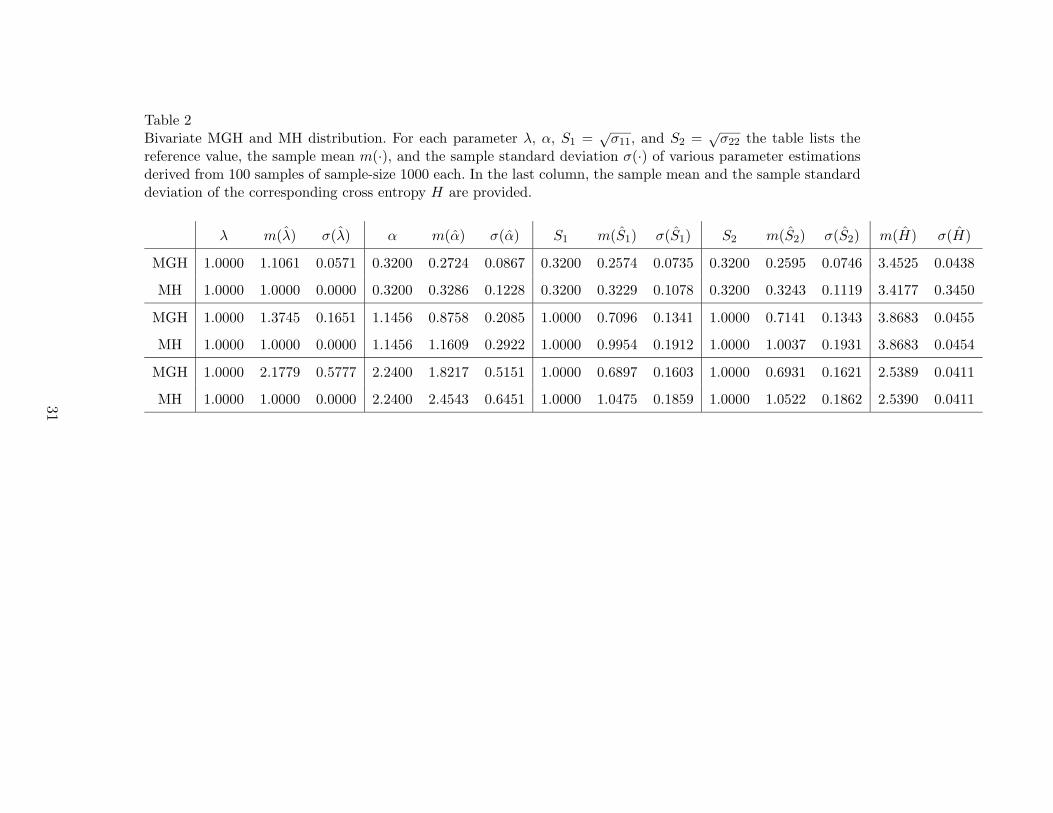
Table 2Bivariate MGH and MH distribution. For each parameter λ, α, S1 =

√σ11, and S2 =

√σ22 the table lists the

reference value, the sample mean m(·), and the sample standard deviation σ(·) of various parameter estimationsderived from 100 samples of sample-size 1000 each. In the last column, the sample mean and the sample standarddeviation of the corresponding cross entropy H are provided.

λ m(λ) σ(λ) α m(α) σ(α) S1 m(S1) σ(S1) S2 m(S2) σ(S2) m(H) σ(H)

MGH 1.0000 1.1061 0.0571 0.3200 0.2724 0.0867 0.3200 0.2574 0.0735 0.3200 0.2595 0.0746 3.4525 0.0438

MH 1.0000 1.0000 0.0000 0.3200 0.3286 0.1228 0.3200 0.3229 0.1078 0.3200 0.3243 0.1119 3.4177 0.3450

MGH 1.0000 1.3745 0.1651 1.1456 0.8758 0.2085 1.0000 0.7096 0.1341 1.0000 0.7141 0.1343 3.8683 0.0455

MH 1.0000 1.0000 0.0000 1.1456 1.1609 0.2922 1.0000 0.9954 0.1912 1.0000 1.0037 0.1931 3.8683 0.0454

MGH 1.0000 2.1779 0.5777 2.2400 1.8217 0.5151 1.0000 0.6897 0.1603 1.0000 0.6931 0.1621 2.5389 0.0411

MH 1.0000 1.0000 0.0000 2.2400 2.4543 0.6451 1.0000 1.0475 0.1859 1.0000 1.0522 0.1862 2.5390 0.041131

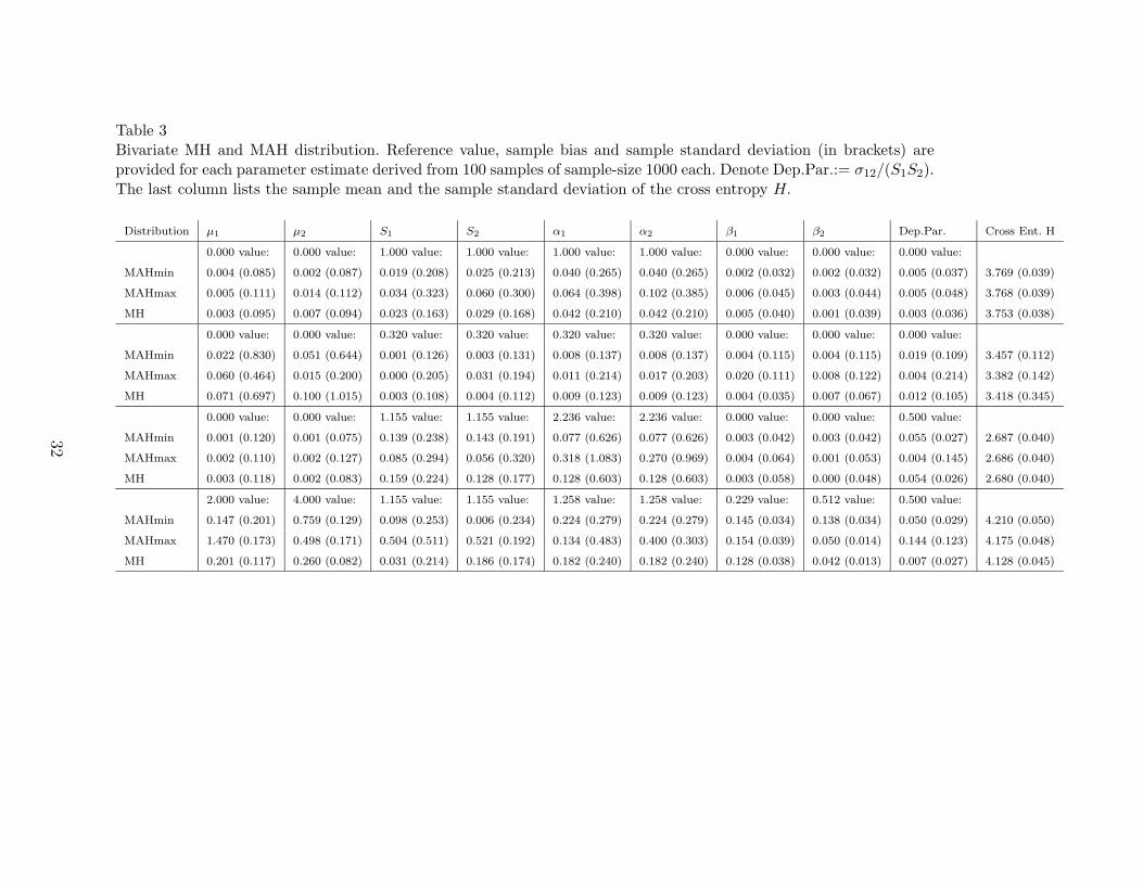
Table 3Bivariate MH and MAH distribution. Reference value, sample bias and sample standard deviation (in brackets) areprovided for each parameter estimate derived from 100 samples of sample-size 1000 each. Denote Dep.Par.:= σ12/(S1S2).The last column lists the sample mean and the sample standard deviation of the cross entropy H.

Distribution µ1 µ2 S1 S2 α1 α2 β1 β2 Dep.Par. Cross Ent. H

0.000 value: 0.000 value: 1.000 value: 1.000 value: 1.000 value: 1.000 value: 0.000 value: 0.000 value: 0.000 value:

MAHmin 0.004 (0.085) 0.002 (0.087) 0.019 (0.208) 0.025 (0.213) 0.040 (0.265) 0.040 (0.265) 0.002 (0.032) 0.002 (0.032) 0.005 (0.037) 3.769 (0.039)

MAHmax 0.005 (0.111) 0.014 (0.112) 0.034 (0.323) 0.060 (0.300) 0.064 (0.398) 0.102 (0.385) 0.006 (0.045) 0.003 (0.044) 0.005 (0.048) 3.768 (0.039)

MH 0.003 (0.095) 0.007 (0.094) 0.023 (0.163) 0.029 (0.168) 0.042 (0.210) 0.042 (0.210) 0.005 (0.040) 0.001 (0.039) 0.003 (0.036) 3.753 (0.038)

0.000 value: 0.000 value: 0.320 value: 0.320 value: 0.320 value: 0.320 value: 0.000 value: 0.000 value: 0.000 value:

MAHmin 0.022 (0.830) 0.051 (0.644) 0.001 (0.126) 0.003 (0.131) 0.008 (0.137) 0.008 (0.137) 0.004 (0.115) 0.004 (0.115) 0.019 (0.109) 3.457 (0.112)

MAHmax 0.060 (0.464) 0.015 (0.200) 0.000 (0.205) 0.031 (0.194) 0.011 (0.214) 0.017 (0.203) 0.020 (0.111) 0.008 (0.122) 0.004 (0.214) 3.382 (0.142)

MH 0.071 (0.697) 0.100 (1.015) 0.003 (0.108) 0.004 (0.112) 0.009 (0.123) 0.009 (0.123) 0.004 (0.035) 0.007 (0.067) 0.012 (0.105) 3.418 (0.345)

0.000 value: 0.000 value: 1.155 value: 1.155 value: 2.236 value: 2.236 value: 0.000 value: 0.000 value: 0.500 value:

MAHmin 0.001 (0.120) 0.001 (0.075) 0.139 (0.238) 0.143 (0.191) 0.077 (0.626) 0.077 (0.626) 0.003 (0.042) 0.003 (0.042) 0.055 (0.027) 2.687 (0.040)

MAHmax 0.002 (0.110) 0.002 (0.127) 0.085 (0.294) 0.056 (0.320) 0.318 (1.083) 0.270 (0.969) 0.004 (0.064) 0.001 (0.053) 0.004 (0.145) 2.686 (0.040)

MH 0.003 (0.118) 0.002 (0.083) 0.159 (0.224) 0.128 (0.177) 0.128 (0.603) 0.128 (0.603) 0.003 (0.058) 0.000 (0.048) 0.054 (0.026) 2.680 (0.040)

2.000 value: 4.000 value: 1.155 value: 1.155 value: 1.258 value: 1.258 value: 0.229 value: 0.512 value: 0.500 value:

MAHmin 0.147 (0.201) 0.759 (0.129) 0.098 (0.253) 0.006 (0.234) 0.224 (0.279) 0.224 (0.279) 0.145 (0.034) 0.138 (0.034) 0.050 (0.029) 4.210 (0.050)

MAHmax 1.470 (0.173) 0.498 (0.171) 0.504 (0.511) 0.521 (0.192) 0.134 (0.483) 0.400 (0.303) 0.154 (0.039) 0.050 (0.014) 0.144 (0.123) 4.175 (0.048)

MH 0.201 (0.117) 0.260 (0.082) 0.031 (0.214) 0.186 (0.174) 0.182 (0.240) 0.182 (0.240) 0.128 (0.038) 0.042 (0.013) 0.007 (0.027) 4.128 (0.045)

32

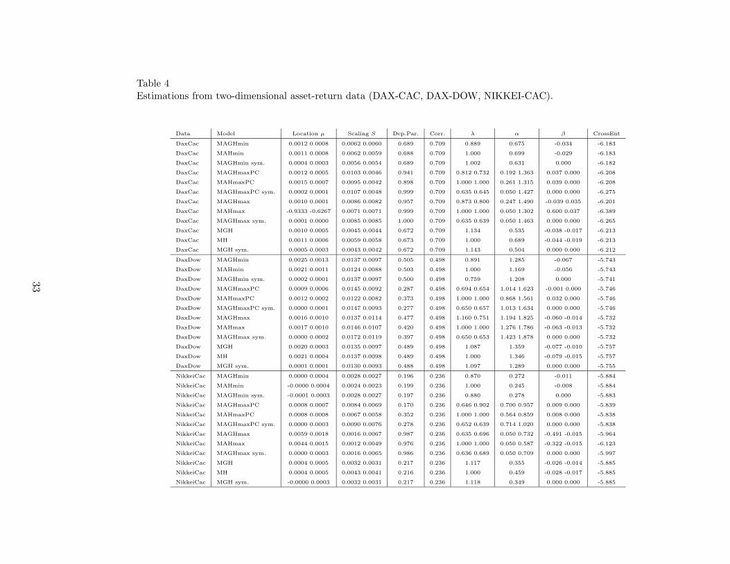
Table 4Estimations from two-dimensional asset-return data (DAX-CAC, DAX-DOW, NIKKEI-CAC).

Data Model Location µ Scaling S Dep.Par. Corr. λ α β CrossEnt

DaxCac MAGHmin 0.0012 0.0008 0.0062 0.0060 0.689 0.709 0.889 0.675 -0.034 -6.183

DaxCac MAHmin 0.0011 0.0008 0.0062 0.0059 0.688 0.709 1.000 0.699 -0.029 -6.183

DaxCac MAGHmin sym. 0.0004 0.0003 0.0056 0.0054 0.689 0.709 1.002 0.631 0.000 -6.182

DaxCac MAGHmaxPC 0.0012 0.0005 0.0103 0.0046 0.941 0.709 0.812 0.732 0.192 1.363 0.037 0.000 -6.208

DaxCac MAHmaxPC 0.0015 0.0007 0.0095 0.0042 0.898 0.709 1.000 1.000 0.261 1.315 0.039 0.000 -6.208

DaxCac MAGHmaxPC sym. 0.0002 0.0001 0.0107 0.0048 0.999 0.709 0.635 0.645 0.050 1.427 0.000 0.000 -6.275

DaxCac MAGHmax 0.0010 0.0001 0.0086 0.0082 0.957 0.709 0.873 0.800 0.247 1.490 -0.039 0.035 -6.201

DaxCac MAHmax -0.9333 -0.6267 0.0071 0.0071 0.999 0.709 1.000 1.000 0.050 1.302 0.600 0.037 -6.389

DaxCac MAGHmax sym. 0.0001 0.0000 0.0085 0.0085 1.000 0.709 0.635 0.639 0.050 1.463 0.000 0.000 -6.265

DaxCac MGH 0.0010 0.0005 0.0045 0.0044 0.672 0.709 1.134 0.535 -0.038 -0.017 -6.213

DaxCac MH 0.0011 0.0006 0.0059 0.0058 0.673 0.709 1.000 0.689 -0.044 -0.019 -6.213

DaxCac MGH sym. 0.0005 0.0003 0.0043 0.0042 0.672 0.709 1.143 0.504 0.000 0.000 -6.212

DaxDow MAGHmin 0.0025 0.0013 0.0137 0.0097 0.505 0.498 0.891 1.285 -0.067 -5.743

DaxDow MAHmin 0.0021 0.0011 0.0124 0.0088 0.503 0.498 1.000 1.169 -0.056 -5.743

DaxDow MAGHmin sym. 0.0002 0.0001 0.0137 0.0097 0.500 0.498 0.759 1.208 0.000 -5.741

DaxDow MAGHmaxPC 0.0009 0.0006 0.0145 0.0092 0.287 0.498 0.694 0.654 1.014 1.623 -0.001 0.000 -5.746

DaxDow MAHmaxPC 0.0012 0.0002 0.0122 0.0082 0.373 0.498 1.000 1.000 0.868 1.561 0.032 0.000 -5.746

DaxDow MAGHmaxPC sym. 0.0000 0.0001 0.0147 0.0093 0.277 0.498 0.650 0.657 1.013 1.634 0.000 0.000 -5.746

DaxDow MAGHmax 0.0016 0.0010 0.0137 0.0114 0.477 0.498 1.160 0.751 1.194 1.825 -0.060 -0.014 -5.732

DaxDow MAHmax 0.0017 0.0010 0.0146 0.0107 0.420 0.498 1.000 1.000 1.276 1.786 -0.063 -0.013 -5.732

DaxDow MAGHmax sym. 0.0000 0.0002 0.0172 0.0119 0.397 0.498 0.650 0.653 1.423 1.878 0.000 0.000 -5.732

DaxDow MGH 0.0020 0.0003 0.0135 0.0097 0.489 0.498 1.087 1.359 -0.077 -0.010 -5.757

DaxDow MH 0.0021 0.0004 0.0137 0.0098 0.489 0.498 1.000 1.346 -0.079 -0.015 -5.757

DaxDow MGH sym. 0.0001 0.0001 0.0130 0.0093 0.488 0.498 1.097 1.289 0.000 0.000 -5.755

NikkeiCac MAGHmin 0.0000 0.0004 0.0028 0.0027 0.196 0.236 0.870 0.272 -0.011 -5.884

NikkeiCac MAHmin -0.0000 0.0004 0.0024 0.0023 0.199 0.236 1.000 0.245 -0.008 -5.884

NikkeiCac MAGHmin sym. -0.0001 0.0003 0.0028 0.0027 0.197 0.236 0.880 0.278 0.000 -5.883

NikkeiCac MAGHmaxPC 0.0008 0.0007 0.0084 0.0069 0.170 0.236 0.646 0.902 0.700 0.957 0.009 0.000 -5.839

NikkeiCac MAHmaxPC 0.0008 0.0008 0.0067 0.0058 0.352 0.236 1.000 1.000 0.564 0.859 0.008 0.000 -5.838

NikkeiCac MAGHmaxPC sym. 0.0000 0.0003 0.0090 0.0076 0.278 0.236 0.652 0.639 0.714 1.020 0.000 0.000 -5.838

NikkeiCac MAGHmax 0.0059 0.0018 0.0016 0.0067 0.987 0.236 0.635 0.696 0.050 0.732 -0.491 -0.015 -5.964

NikkeiCac MAHmax 0.0044 0.0015 0.0012 0.0049 0.976 0.236 1.000 1.000 0.050 0.587 -0.322 -0.015 -6.123

NikkeiCac MAGHmax sym. 0.0000 0.0003 0.0016 0.0065 0.986 0.236 0.636 0.689 0.050 0.709 0.000 0.000 -5.997

NikkeiCac MGH 0.0004 0.0005 0.0032 0.0031 0.217 0.236 1.117 0.355 -0.026 -0.014 -5.885

NikkeiCac MH 0.0004 0.0005 0.0043 0.0041 0.216 0.236 1.000 0.459 -0.028 -0.017 -5.885

NikkeiCac MGH sym. -0.0000 0.0003 0.0032 0.0031 0.217 0.236 1.118 0.349 0.000 0.000 -5.885

33

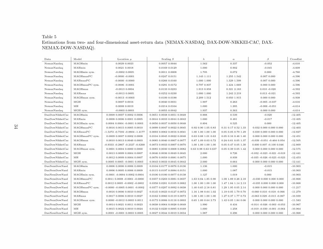
Table 5Estimations from two- and four-dimensional asset-return data (NEMAX-NASDAQ, DAX-DOW-NIKKEI-CAC, DAX-NEMAX-DOW-NASDAQ).

Data Model Location µ Scaling S λ α β CrossEnt

NemaxNasdaq MAGHmin 0.0029 0.0023 0.0057 0.0044 1.562 0.337 -0.052 -4.610

NemaxNasdaq MAHmin 0.0021 0.0018 0.0169 0.0129 1.000 0.902 -0.045 -4.609

NemaxNasdaq MAGHmin sym. -0.0002 0.0005 0.0011 0.0008 1.705 0.072 0.000 -4.760

NemaxNasdaq MAGHmaxPC -0.0000 -0.0001 0.0247 0.0151 1.143 1.111 1.255 1.542 0.007 0.000 -4.596

NemaxNasdaq MAHmaxPC -0.0000 -0.0000 0.0266 0.0160 1.000 1.000 1.329 1.599 0.007 0.000 -4.596

NemaxNasdaq MAGHmaxPC sym. -0.0006 -0.0001 0.0291 0.0172 0.797 0.837 1.424 1.669 0.000 0.000 -4.596

NemaxNasdaq MAGHmax -0.0013 0.0004 0.0133 0.0233 1.913 0.858 0.321 2.183 0.010 -0.020 -4.592

NemaxNasdaq MAHmax -0.0013 0.0005 0.0252 0.0230 1.000 1.000 1.242 2.219 0.013 -0.021 -4.592

NemaxNasdaq MAGHmax sym. -0.0013 -0.0003 0.0100 0.0188 2.209 1.512 0.050 1.915 0.000 0.000 -4.938

NemaxNasdaq MGH 0.0007 0.0016 0.0040 0.0031 1.907 0.263 -0.005 -0.037 -4.616

NemaxNasdaq MH 0.0008 0.0019 0.0214 0.0164 1.000 1.205 -0.006 -0.051 -4.614

NemaxNasdaq MGH sym. -0.0003 0.0003 0.0055 0.0042 1.937 0.363 0.000 0.000 -4.614

DaxDowNikkeiCac MAGHmin 0.0009 0.0007 0.0002 0.0006 0.0051 0.0038 0.0051 0.0049 0.888 0.539 -0.020 -12.405

DaxDowNikkeiCac MAHmin 0.0008 0.0006 0.0001 0.0005 0.0044 0.0033 0.0044 0.0042 1.000 0.481 -0.017 -12.405

DaxDowNikkeiCac MAGHmin sym. 0.0004 0.0004 -0.0001 0.0003 0.0050 0.0037 0.0050 0.0048 0.894 0.525 0.000 -12.405

DaxDowNikkeiCac MAGHmaxPC 0.0016 0.0015 0.0005 0.0010 0.0099 0.0047 0.0022 0.0045 0.92 0.90 1.05 0.83 0.31 0.17 0.52 1.33 0.032 0.000 0.000 0.000 -12.403

DaxDowNikkeiCac MAHmaxPC -1.5272 -0.7592 -0.8804 -1.4177 0.0093 0.0062 0.0016 0.0041 1.00 1.00 1.00 1.00 0.05 0.05 0.79 1.29 0.039 0.000 0.000 0.000 -12.827

DaxDowNikkeiCac MAGHmaxPC sym. 0.0009 0.0007 0.0002 0.0008 0.0104 0.0045 0.0022 0.0048 0.63 0.88 1.01 0.63 0.05 0.16 0.46 1.40 0.000 0.000 0.000 0.000 -12.451

DaxDowNikkeiCac MAGHmax 0.0010 0.0013 0.0049 0.0003 0.0085 0.0040 0.0007 0.0077 0.87 1.09 0.63 0.72 0.24 0.61 0.05 1.37 -0.039 -0.051 -0.464 0.054 -12.505

DaxDowNikkeiCac MAHmax -0.9333 -0.2867 -0.2327 -0.6268 0.0073 0.0033 0.0007 0.0070 1.00 1.00 1.00 1.00 0.05 0.47 0.05 1.30 0.600 0.007 -0.100 0.046 -12.869

DaxDowNikkeiCac MAGHmax sym. 0.0001 0.0004 0.0000 0.0000 0.0085 0.0030 0.0008 0.0082 0.63 0.98 0.63 0.637 0.05 0.39 0.05 1.42 0.000 0.000 0.000 0.000 -12.575

DaxDowNikkeiCac MGH 0.0013 0.0009 0.0004 0.0007 0.0046 0.0036 0.0049 0.0045 2.000 0.726 -0.032 -0.023 -0.021 -0.019 -12.441

DaxDowNikkeiCac MH 0.0012 0.0009 0.0004 0.0007 0.0076 0.0059 0.0081 0.0075 1.000 0.939 -0.035 -0.026 -0.023 -0.023 -12.453

DaxDowNikkeiCac MGH sym. 0.0005 0.0005 -0.0001 0.0003 0.0043 0.0033 0.0045 0.0042 2.000 0.664 0.000 0.000 0.000 0.000 -12.441

DaxNemDowNasd MAGHmin 0.0006 0.0006 0.0006 0.0009 0.0104 0.0177 0.0076 0.0136 1.136 1.000 -0.015 -10.903

DaxNemDowNasd MAHmin 0.0006 0.0005 0.0006 0.0009 0.0115 0.0197 0.0084 0.0151 1.000 1.087 -0.015 -10.903

DaxNemDowNasd MAGHmin sym. -0.0001 -0.0004 0.0002 0.0004 0.0106 0.0180 0.0077 0.0138 1.127 1.019 0.000 -10.903

DaxNemDowNasd MAGHmaxPC 0.0011 0.0008 -0.0001 -0.0000 0.0357 0.0203 0.0081 0.0037 1.63 0.84 1.85 0.90 1.08 1.89 0.26 2.18 -0.030 0.000 0.000 0.000 -10.868

DaxNemDowNasd MAHmaxPC 0.0012 0.0005 -0.0002 -0.0002 0.0358 0.0201 0.0105 0.0062 1.00 1.00 1.00 1.00 1.47 1.84 1.14 2.13 -0.035 0.000 0.000 0.000 -10.868

DaxNemDowNasd MAGHmaxPC sym. -0.0000 -0.0005 0.0001 -0.0002 0.0377 0.0207 0.0092 0.0038 1.40 0.65 2.18 0.81 1.29 1.95 0.05 2.14 0.000 0.000 0.000 0.000 -11.217

DaxNemDowNasd MAGHmax 0.0016 0.0006 0.0010 0.0027 0.0145 0.0023 0.0127 0.0072 1.16 1.98 0.64 1.02 1.19 0.05 1.79 0.70 -0.060 0.010 -0.018 -0.066 -11.279

DaxNemDowNasd MAHmax 0.0017 0.0006 0.0010 0.0027 0.0162 0.0060 0.0119 0.0073 1.00 1.00 1.00 1.00 1.27 0.37 1.77 0.72 -0.063 0.029 -0.013 -0.067 -10.939

DaxNemDowNasd MAGHmax sym. 0.0000 -0.0012 0.0002 0.0011 0.0172 0.0006 0.0118 0.0003 0.65 1.89 0.64 2.73 1.42 0.05 1.84 0.06 0.000 0.000 0.000 0.000 -11.583

DaxNemDowNasd MGH 0.0014 0.0021 0.0011 0.0023 0.0038 0.0064 0.0028 0.0049 1.990 0.434 -0.014 -0.026 -0.003 -0.053 -10.967

DaxNemDowNasd MH 0.0015 0.0022 0.0010 0.0024 0.0132 0.0220 0.0095 0.0169 1.000 1.258 -0.019 -0.030 -0.001 -0.064 -10.964

DaxNemDowNasd MGH sym. 0.0001 -0.0001 0.0003 0.0005 0.0027 0.0044 0.0019 0.0034 1.987 0.296 0.000 0.000 0.000 0.000 -10.968

34