estimation of the multivariate conditional-tail...
TRANSCRIPT

Introduction Multivariate Conditional-Tail-Expectation Estimation Simulation Study Rainfall real data Perspectives Appendix
Estimation of the Multivariate Conditional-Tail-Expectationfor extreme risk levels: illustration on a rainfall data-set
Elena Di Bernardino
Joint work with Clémentine Prieur
GT Valeurs Extrêmes, Université Paris 6
April 14, 2015
1 / 49Estimation of extreme multivariate Conditional-Tail-Expectation
N

Introduction Multivariate Conditional-Tail-Expectation Estimation Simulation Study Rainfall real data Perspectives Appendix
Contents
1 Introduction
2 Multivariate Conditional-Tail-Expectation
3 EstimationEstimation procedure: A two-stage approach
Asymptotic normality
4 Simulation Study
5 Rainfall real data
6 Perspectives
2 / 49Estimation of extreme multivariate Conditional-Tail-Expectation
N

Introduction Multivariate Conditional-Tail-Expectation Estimation Simulation Study Rainfall real data Perspectives Appendix
1 Introduction
2 Multivariate Conditional-Tail-Expectation
3 EstimationEstimation procedure: A two-stage approach
Asymptotic normality
4 Simulation Study
5 Rainfall real data
6 Perspectives
3 / 49Estimation of extreme multivariate Conditional-Tail-Expectation
N

Introduction Multivariate Conditional-Tail-Expectation Estimation Simulation Study Rainfall real data Perspectives Appendix
Multivariate risk problems require multivariatemeasures
Financial risks are strongly interconnected and cannot be managed individually
Construction of risk measures that account both for marginal e�ects anddependence between risks
Multivariate risk measures involve in di�erent applications
1) Capital allocation problem
2) Measures of systemic risk
3) Measures for risks with heterogeneous characteristics
4) Environmental multivariate risks
4 / 49Estimation of extreme multivariate Conditional-Tail-Expectation
N

Introduction Multivariate Conditional-Tail-Expectation Estimation Simulation Study Rainfall real data Perspectives Appendix
(Multivariate) Return Period
The notion of Return Period (RP) is frequently used in environmental sciences forthe identi�cation of dangerous events, and provides a means for rational decisionmaking and risk assessment.
Roughly speaking, the RP can be considered as an analogue of the �Value-at-Risk�in Economics and Finance, since it is used to quantify and assess the risk.
During the last years, researchers in environmental �elds joined e�orts to properlyanswer the following crucial question: �How is it possible to calculate the criticaldesign event(s) in the multivariate case?�.
5 / 49Estimation of extreme multivariate Conditional-Tail-Expectation
N
Introduction Multivariate Conditional-Tail-Expectation Estimation Simulation Study Rainfall real data Perspectives Appendix
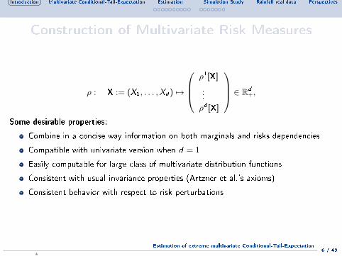
Construction of Multivariate Risk Measures
ρ : X := (X1, . . . ,Xd ) 7→
ρ1[X]
...
ρd [X]
∈ Rd+,
Some desirable properties:
Combine in a concise way information on both marginals and risks dependencies
Compatible with univariate version when d = 1
Easily computable for large class of multivariate distribution functions
Consistent with usual invariance properties (Artzner et al.'s axioms)
Consistent behavior with respect to risk perturbations
6 / 49Estimation of extreme multivariate Conditional-Tail-Expectation
N

Introduction Multivariate Conditional-Tail-Expectation Estimation Simulation Study Rainfall real data Perspectives Appendix
Capital allocation problem
X = (X1, . . . ,Xd ) : risk exposures of a given �nancial institution
Xj : risk exposure of underlying entity j (could be a subsidiary, an operationalbranch, a risk category)
Capital charge is measured from the aggregated risk
L = X1 + · · ·+ Xd
What is the contribution of each subsidiary ?
Euler (or Shapley-Aumann) allocation rule involves both Xi and L:
VaRα(Xi | L) = E[Xi | L = VaRα(L) ], i = 1, . . . , d
ESα(Xi | L) = E[Xi | L ≥ VaRα(L) ], i = 1, . . . , d
Scaillet (2004), Tasche (2008)
7 / 49Estimation of extreme multivariate Conditional-Tail-Expectation
N

Introduction Multivariate Conditional-Tail-Expectation Estimation Simulation Study Rainfall real data Perspectives Appendix
Other types of multivariate risk measures
Other risk measures based on function min or max have been proposed:
CTEminα (Xi ) = E[Xi |X(1) ≥ QX(1)
(α) ], where X(1) = min{X1, ...,Xd}
CTEmaxα (Xi ) = E[Xi |X(d) ≥ QX(d )
(α) ], where X(d) = max{X1, ...,Xd}
Landsman and Valdez (2003): elliptical distribution functions
Cai and Li (2005): phase-type distributions
Bargès, Cossette, Marceau (2009): Farlie-Gumbel-Morgenstern copulas
8 / 49Estimation of extreme multivariate Conditional-Tail-Expectation
N

Introduction Multivariate Conditional-Tail-Expectation Estimation Simulation Study Rainfall real data Perspectives Appendix
Measures of Systemic Risks
Systemic risk in an interconnected network of �nancial institutions
X = (X1, . . . ,Xd ) where Xj is the risk exposure of company j .
L = X1 + · · ·+ Xd represents the aggregated risk in the �rm network
The CoVaR associated with company i
CoVaRiα(X ) = VaRα (L | Xi ≥ VaRα(Xi ))
Adrian and Brunnermeier (2011), Mainik and Schaanning (2012), Di Bernardino etal. (2014)
The Marginal Expected Shortfall (MES) for the systemic risk, de�ned as theexpected loss on its equity return (X ) conditional on the occurrence of a loss in theaggregated return of the �nancial sector (Y ), i.e.,
MESα(X ) = E[X |Y > QY (α)],
see Cai et al. (2015).
9 / 49Estimation of extreme multivariate Conditional-Tail-Expectation
N

Introduction Multivariate Conditional-Tail-Expectation Estimation Simulation Study Rainfall real data Perspectives Appendix
Measures for risk with heterogeneouscharacteristics
Risks that cannot be aggregated together
↪→ Hydrological variables can be of di�erent nature (e.g. precipitation,temperature, discharge, . . . ), prohibiting the aggregation of thevarious components.
↪→ A �ood, e.g., can be described by three main characteristics: thepeak �ow, the volume and the duration.
In this sense, a possible consistent theoretical framework for the calculation of thedesign event(s) and the associated return period(s) in a multi-dimensionalenvironment, is proposed, e.g., by Salvadori et al.(2011), Chebana and Ouarda(2011), Salvadori et al.(2012), Gräler et al. (2013).
X Multivariate return period using the notion of upper and lower levelsets of multivariate probability distribution F and of the associatedKendall's measure.
10 / 49Estimation of extreme multivariate Conditional-Tail-Expectation
N

Introduction Multivariate Conditional-Tail-Expectation Estimation Simulation Study Rainfall real data Perspectives Appendix
1 Introduction
2 Multivariate Conditional-Tail-Expectation
3 EstimationEstimation procedure: A two-stage approach
Asymptotic normality
4 Simulation Study
5 Rainfall real data
6 Perspectives
11 / 49Estimation of extreme multivariate Conditional-Tail-Expectation
N
Introduction Multivariate Conditional-Tail-Expectation Estimation Simulation Study Rainfall real data Perspectives Appendix
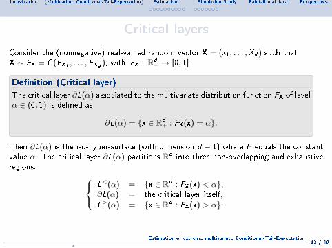
Critical layers
Consider the (nonnegative) real-valued random vector X = (x1, . . . ,Xd ) such thatX ∼ FX = C(FX1 , . . . ,FXd ), with FX : Rd
+ → [0, 1].
De�nition (Critical layer)
The critical layer ∂L(α) associated to the multivariate distribution function FX of levelα ∈ (0, 1) is de�ned as
∂L(α) = {x ∈ Rd+ : FX(x) = α}.
Then ∂L(α) is the iso-hyper-surface (with dimension d − 1) where F equals the constantvalue α. The critical layer ∂L(α) partitions Rd into three non-overlapping and exhaustiveregions:
L<(α) = {x ∈ Rd : FX(x) < α},∂L(α) = the critical layer itself,
L>(α) = {x ∈ Rd : FX(x) > α}.
12 / 49Estimation of extreme multivariate Conditional-Tail-Expectation
N

Introduction Multivariate Conditional-Tail-Expectation Estimation Simulation Study Rainfall real data Perspectives Appendix
Multivariate RP and Critical layers
Event of interest is of the type {X ∈ A}, where A is a non-empty Borel set in Rd
collecting all the values judged to be �dangerous� according to some suitable criterion.
X A natural choice for A is the set L>(α)
X Then RP>(α) = ∆tP[X∈L>(α)]
, where ∆t > 0 is the (deterministic) average
time elapsing between Xk and Xk+1, k ∈ N.
Then, the considered Return Period can be expressed using Kendall's function
RP>(α) = ∆t ·
1
1− KC (α),
where KC (α) = P[X ∈ L<(α)
]= P [C(U1, . . . ,Ud ) ≤ α] , for α ∈ (0, 1).
13 / 49Estimation of extreme multivariate Conditional-Tail-Expectation
N

Introduction Multivariate Conditional-Tail-Expectation Estimation Simulation Study Rainfall real data Perspectives Appendix
Multivariate CTE-s based on upper-level set of multivariate cdf and lower-level set ofsurvival functions:
L(α) = {x ∈ Rd+ : F (x) ≥ α} L(α) = {x ∈ Rd
+ : F (x) ≤ 1− α}
0.10.1
0.1
0.10.1
0.20.2
0.20.2
0.30.3
0.3
0.4
0.4
0.4
0.5
0.5
0.6
0.6
0.7
0.8
0.9
u
v
0 0.1 0.2 0.3 0.4 0.5 0.6 0.7 0.8 0.9 10
0.1
0.2
0.3
0.4
0.5
0.6
0.7
0.8
0.9
1
0.1 0.10.1
0.10.1
0.20.2
0.20.2
0.30.3
0.3
0.4
0.4
0.4
0.5
0.5
0.6
0.6
0.7
0.80.9
uv
0 0.1 0.2 0.3 0.4 0.5 0.6 0.7 0.8 0.9 10
0.1
0.2
0.3
0.4
0.5
0.6
0.7
0.8
0.9
1
Figure : left: quantile curves of Frank copula with parameter 4; right: quantile curves ofthe associated survival distribution function
14 / 49Estimation of extreme multivariate Conditional-Tail-Expectation
N

Introduction Multivariate Conditional-Tail-Expectation Estimation Simulation Study Rainfall real data Perspectives Appendix
de Haan and Huang (1995) model a risk-problem of �ood in the bivariate settingusing an estimator of level curves ∂L(α) of the bivariate distribution function.
Furthermore, as noticed by Embrechts and Puccetti (2006), it can be viewed as anatural multivariate version of the univariate quantile. The interested reader is alsoreferred to Tibiletti (1993), Belzunce et al. (2007), Nappo and Spizzichino (2009),Prékopa (2010), Lee and Prékopa (2012).
In the following we deal with a version of the multivariateConditional-Tail-Expectation, previously proposed by Di Bernardino et al. 2013 (seealso Cousin and Di Bernardino, 2014; Di Bernardino and Prieur, 2014). It isconstructed as the conditional expectation of a d−dimensional vector of risksX = (X 1,X 2, . . . ,X d ) following the distribution function F , given that theassociated multivariate probability integral transformation Z = F (X) is large.
15 / 49Estimation of extreme multivariate Conditional-Tail-Expectation
N

Introduction Multivariate Conditional-Tail-Expectation Estimation Simulation Study Rainfall real data Perspectives Appendix
Lower-Orthant and Upper-Orthant CTE
De�nition
Consider a random vector X with absolutely continuous cdf F and survival functionF . For α ∈ (0, 1), we de�ne:
CTEα(X) := E[X|F (X) ≥ α] =
E[X1 |F (X) ≥ α ]
...
E[Xd |F (X) ≥ α ]
CTEα(X) := E[X|F (X) ≤ 1− α] =
E[X1 |F (X) ≤ 1− α ]
...
E[Xd |F (X) ≤ 1− α ]
When d = 1: CTEα(X ) = CTEα(X ) = CTEα(X )
16 / 49Estimation of extreme multivariate Conditional-Tail-Expectation
N
Introduction Multivariate Conditional-Tail-Expectation Estimation Simulation Study Rainfall real data Perspectives Appendix
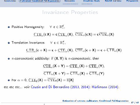
Invariance Properties
Positive Homogeneity: ∀ c ∈ Rd+,
CTEα(cX) = cCTEα(X), CTEα(cX) = cCTEα(X)
Translation Invariance: ∀ c ∈ Rd+,
CTEα(c + X) = c + CTEα(X), CTEα(c + X) = c + CTEα(X)
π-comonotonic additivity: if (X,Y) is π-comonotonic, then
CTEα(X + Y) = CTEα(X) + CTEα(Y),
CTEα(X + Y) = CTEα(X) + CTEα(Y)
For α = 0, CTE0(X) = CTE0(X) = E[X]
etc etc etc... voir Cousin and Di Bernardino (2013, 2014); Hürlimann (2014).
17 / 49Estimation of extreme multivariate Conditional-Tail-Expectation
N

Introduction Multivariate Conditional-Tail-Expectation Estimation Simulation Study Rainfall real data Perspectives Appendix
De�ne Z := F (X), with X = (X 1,X 2, . . . ,X d ) and the associated multivariate Kendalldistribution function K(t) = P[Z ≤ t], for t ∈ [0, 1]. 1
As a consequence of Sklar's Theorem, the Kendall distribution only depends on thedependence structure or the copula function C associated with X. Thus, we also have
K(t) = P[C(V) ≤ t],
where V = (V1, . . . ,Vd ) with uniform marginals V1 = FX1(X 1), . . . ,Vd = FXd (X d ).
Furthermore t ≤ K(t) ≤ 1, for all t ∈ (0, 1).
Copula Kendall distribution K(t)
Archimedean case t +∑d−1
i=11i !
(−φ(t))i(φ−1
)(i)(φ(t))
Counter-monotonic case (d = 2) 1
Independent case t + t∑d−1
i=1
(ln(1/t)i
i !
)Comonotonic case t
1For more details on the multivariate probability integral transformation see Capéeràa et al.(1997), Genest and Rivest (2001), Nelsen et al. (2003), Genest et al. (2006).
18 / 49Estimation of extreme multivariate Conditional-Tail-Expectation
N

Introduction Multivariate Conditional-Tail-Expectation Estimation Simulation Study Rainfall real data Perspectives Appendix
1 Introduction
2 Multivariate Conditional-Tail-Expectation
3 EstimationEstimation procedure: A two-stage approach
Asymptotic normality
4 Simulation Study
5 Rainfall real data
6 Perspectives
19 / 49Estimation of extreme multivariate Conditional-Tail-Expectation
N

Introduction Multivariate Conditional-Tail-Expectation Estimation Simulation Study Rainfall real data Perspectives Appendix
We aim to estimate the quantity
θip := E[X i |Z > QZ (1− p)] = E[X i |Z > UZ (1/p)], for p ∈ (0, 1)
where UZ = ( 11−K )← is the tail quantile function of Z .
Assumptions:
- For all (x , z) ∈ [0,∞]2 \ {(∞,∞)}, and for all i = 1, . . . , d , the following limitsexist:
limt→∞
t P[1− Fi (X
i ) ≤ x
t, 1− K(Z) ≤ z
t
]:= R(X i ,Z)(x , z).
Remark that the function R(Xi ,Z)
completely determines the so-called stable tail dependence
function l(Xi ,Z)
, as for all x, z ≥ 0,
l(Xi ,Z)
(x, z) = x + z − R(Xi ,Z)
(x, z),
(see, e.g., Drees and Huang, 1998; Beirlant et al., 2004).
- There exists γ i > 0 such that for all x > 0,
limt→∞
Ui (tx)
Ui (t)= xγ
i
.
Then X i follows a distribution with a heavy right tail, i.e., 1− Fi is regularly varying with index
−1/γi and γi is the extreme value index.
20 / 49Estimation of extreme multivariate Conditional-Tail-Expectation
N

Introduction Multivariate Conditional-Tail-Expectation Estimation Simulation Study Rainfall real data Perspectives Appendix
Estimation procedure: A two-stage approach
Let n1 and n2 ∈ N∗ and n = n1 + n2.
We consider (Xj )j=1,...,n a d−dimensional i.i.d. sample of X.
For all t ∈ Rd+ we de�ne the d−dimensional empirical distribution function of X based on
n2 observations of this sample as,
Fn2(t) =1
n2
n1+n2∑j=n1+1
1{Xj ≤ t}.
For all j = 1, . . . , n1 we de�ne Zj = F (Xj ) and Z̃j = Fn2(Xj ).
Following classical extrapolation techniques of EVT, we construct an estimator of θip, for
i = 1, . . . , d , by a two-stage approach.
21 / 49Estimation of extreme multivariate Conditional-Tail-Expectation
N
Introduction Multivariate Conditional-Tail-Expectation Estimation Simulation Study Rainfall real data Perspectives Appendix
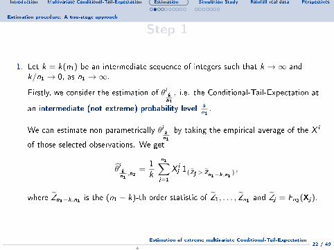
Estimation procedure: A two-stage approach
Step 1
1. Let k = k(n1) be an intermediate sequence of integers such that k →∞ andk/n1 → 0, as n1 →∞.
Firstly, we consider the estimation of θi kn1
, i.e. the Conditional-Tail-Expectation at
an intermediate (not extreme) probability level kn1.
We can estimate non-parametrically θi kn1
by taking the empirical average of the X i
of those selected observations. We get
θ̂i kn1,n2
=1
k
n1∑j=1
X ij 1{Z̃j > Z̃n1−k,n1
},
where Z̃n1−k,n1 is the (n1 − k)-th order statistic of Z̃1, . . . , Z̃n1 and Z̃j = Fn2(Xj ).
22 / 49Estimation of extreme multivariate Conditional-Tail-Expectation
N

Introduction Multivariate Conditional-Tail-Expectation Estimation Simulation Study Rainfall real data Perspectives Appendix
Estimation procedure: A two-stage approach
Step 2
2. Using an extrapolation method based on our assumptions, we have, for n1 →∞,
θip ∼Ui (1/p)
Ui (n1/k)θi kn1
∼(
k
n1 p
)γiθi kn1
.
In order to apply this asymptotic approximation, we need to estimate γ i .
To this aim, we will consider the Hill estimator (see Hill, 1975), i.e.
γ̂ i =1
k1
k1∑j=1
ln(X in1−j+1,n1)− ln(X i
n1−k1,n1),
where k1 = k1(n1) is an intermediate sequence of integers and X ij,n1 , for
j = 1, . . . , n1, is the j-th order statistic of X i1, . . . ,X
in1 .
23 / 49Estimation of extreme multivariate Conditional-Tail-Expectation
N
Introduction Multivariate Conditional-Tail-Expectation Estimation Simulation Study Rainfall real data Perspectives Appendix
Estimation procedure: A two-stage approach
Final estimator
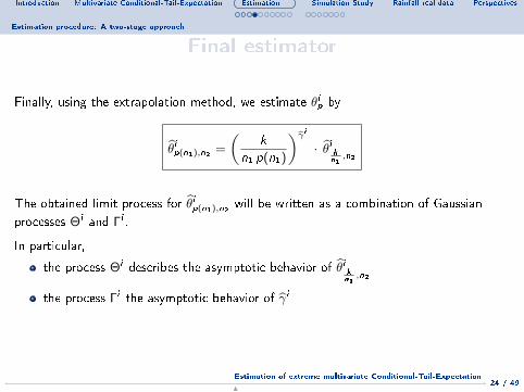
Finally, using the extrapolation method, we estimate θip by
θ̂ip(n1),n2 =
(k
n1 p(n1)
)γ̂i· θ̂i k
n1,n2
The obtained limit process for θ̂ip(n1),n2will be written as a combination of Gaussian
processes Θi and Γi .
In particular,
the process Θi describes the asymptotic behavior of θ̂i kn1,n2
the process Γi the asymptotic behavior of γ̂ i
24 / 49Estimation of extreme multivariate Conditional-Tail-Expectation
N
Introduction Multivariate Conditional-Tail-Expectation Estimation Simulation Study Rainfall real data Perspectives Appendix
Asymptotic normality
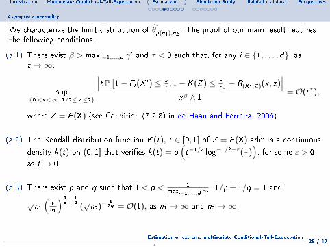
We characterize the limit distribution of θ̂ip(n1),n2. The proof of our main result requires
the following conditions:
(a.1) There exist β > maxi=1,...,d γi and τ < 0 such that, for any i ∈ {1, . . . , d}, as
t →∞.
sup{0<x<∞, 1/2≤ z ≤2}
∣∣∣t P [1− Fi (Xi ) ≤ x
t, 1− K(Z) ≤ z
t
]− R(X i ,Z)(x , z)
∣∣∣xβ ∧ 1
= O(tτ ),
where Z = F (X) (see Condition (7.2.8) in de Haan and Ferreira, 2006).
(a.2) The Kendall distribution function K(t), t ∈ [0, 1] of Z = F (X) admits a continuous
density k(t) on (0, 1] that veri�es k(t) = o(t−1/2 log−1/2−ε( 1
t)), for some ε > 0
as t → 0.
(a.3) There exist p and q such that 1 < p < 1maxi=1,...,d γi
, 1/p + 1/q = 1 and
√n1(
kn1
) 1p−
12
(√n2)−
12q = O(1), as n1 →∞ and n2 →∞.
25 / 49Estimation of extreme multivariate Conditional-Tail-Expectation
N

Introduction Multivariate Conditional-Tail-Expectation Estimation Simulation Study Rainfall real data Perspectives Appendix
Asymptotic normality
(b) For i ∈ {1, . . . , d}, there exist ρi < 0 and an eventually positive or negativefunction Ai such that as t →∞, Ai (t x)/Ai (t)→ xρi for all x > 0 and
supx>1
|x−γi Ui (t x)
Ui (t)− 1| = O(Ai (t)),
(see Condition (3.2.4) in de Haan and Ferreira, 2006).
(c) For i ∈ {1, . . . , d}, as n1 →∞,√k1 Ai (n1/k1)→ 0, where k1(n1) is the
intermediate sequence of integers considered before.
(d) For i ∈ {1, . . . , d}, as n1 →∞, k = O(nα1 ) for some
α < min(−2 τ−2 τ+1
, 2 γi ρi2 γi ρi+ρi−1
), where k(n1) is the intermediate sequence of
integers considered before.
26 / 49Estimation of extreme multivariate Conditional-Tail-Expectation
N

Introduction Multivariate Conditional-Tail-Expectation Estimation Simulation Study Rainfall real data Perspectives Appendix
Asymptotic normality
Remarks
- Assumption (a.1) is a second order strengthening of the condition on R(X i ,Z). It isclassically required in EV theory to derive a central limit theorem. Note that thissecond order assumption is required on the bivariate vectors (X i ,Z), whereZ = F (X). Moreover, the constants β and τ do not depend on i ∈ {1, . . . , d}.
- Assumption (a.2) is a regularity assumption on the Kendall density k(t). Thisassumption was necessary in Barbe et al. (2006) to guarantee the convergence ofthe empirical Kendall process. In our proofs, it is required as our estimator is basedon (X i , Z̃) and not on the vector (X i ,Z) itself, as the component Z can not beobserved. Note that this assumption is satis�ed for a large class of multivariatedistributions, as the class of Archimedean copulas, bivariate extreme copulas,Farlie-Gumbel-Morgenstern class of distributions . . . (see Section 3 in Barbe et al.(2006)).
- Assumption (a.3) describes the relationship between the sample sizes n1 and n2.
- Assumption (b) is a second order strengthening of the tail behaviour of X i .
- Assumptions (c) and (d) deal with the intermediate sequences k1 and k respectively.
27 / 49Estimation of extreme multivariate Conditional-Tail-Expectation
N
Introduction Multivariate Conditional-Tail-Expectation Estimation Simulation Study Rainfall real data Perspectives Appendix
Asymptotic normality
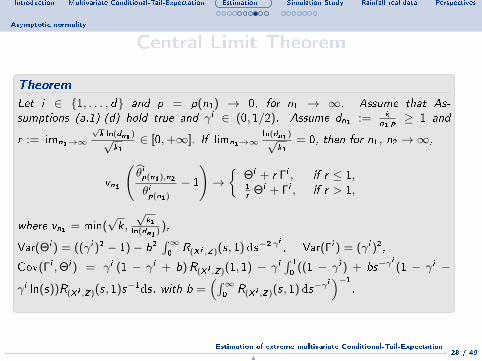
Central Limit Theorem
Theorem
Let i ∈ {1, . . . , d} and p = p(n1) → 0, for n1 → ∞. Assume that As-sumptions (a.1)-(d) hold true and γ i ∈ (0, 1/2). Assume dn1 := k
n1 p≥ 1 and
r := limn1→∞
√k ln(dn1 )√
k1∈ [0,+∞]. If limn1→∞
ln(dn1 )√k1
= 0, then for n1, n2 →∞,
vn1
(θ̂ip(n1),n2
θip(n1)
− 1
)→{
Θi + r Γi , if r ≤ 1,1r
Θi + Γi , if r > 1,
where vn1 = min(√k,
√k1
ln(dn1 )),
Var(Θi ) = ((γ i )2 − 1)− b2∫∞0
R(X i ,Z)(s, 1)ds−2 γi, Var(Γi ) = (γ i )2,
Cov(Γi ,Θi ) = γ i (1 − γ i + b)R(X i ,Z)(1, 1) − γ i∫ 10
((1 − γ i ) + bs−γi(1 − γ i −
γ i ln(s))R(X i ,Z)(s, 1)s−1ds, with b =(∫∞
0R(X i ,Z)(s, 1) ds−γ
i)−1
.
28 / 49Estimation of extreme multivariate Conditional-Tail-Expectation
N
Introduction Multivariate Conditional-Tail-Expectation Estimation Simulation Study Rainfall real data Perspectives Appendix
Asymptotic normality
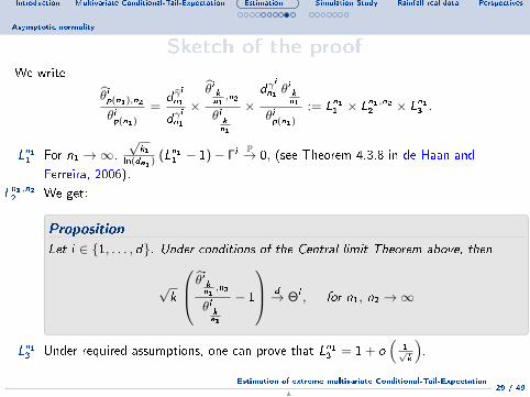
Sketch of the proofWe write
θ̂ip(n1),n2
θip(n1)
=d γ̂
i
n1
dγi
n1
×θ̂i kn1,n2
θikn1
×dγ
i
n1 θikn1
θip(n1)
:= Ln11 × Ln1,n22 × Ln13 .
Ln11 For n1 →∞,
√k1
ln(dn1 )(Ln11 − 1)− Γi
P→ 0, (see Theorem 4.3.8 in de Haan and
Ferreira, 2006).
Ln1,n22 We get:
Proposition
Let i ∈ {1, . . . , d}. Under conditions of the Central limit Theorem above, then
√k
θ̂i kn1 ,n2θi
kn1
− 1
d→ Θi , for n1, n2 →∞
Ln13 Under required assumptions, one can prove that Ln13 = 1 + o(
1√k
).
29 / 49Estimation of extreme multivariate Conditional-Tail-Expectation
N

Introduction Multivariate Conditional-Tail-Expectation Estimation Simulation Study Rainfall real data Perspectives Appendix
Asymptotic normality
RemarksWe discuss here two problematic points in the assumptions of our Central limit Theorem.
1. Assumption (a.1) excludes asymptotic independence, i.e., R(X i ,Z) ≡ 0.
2. Let i ∈ {1, . . . , d}. The assumption γ i ∈ (0, 1/2) is necessary, i.e., the result does
not hold true when γ i = 1/2. For the consistency of θ̂ip(n1),n2this assumption can
be relaxed to γ i ∈ (0, 1).
Proposition
Assume that (X i ,Z) satis�es Assumptions on R(X i ,Z) and (b), R(X i , Z̃)(1, 1) > 0,
limn1→∞log(dn1 )√
k1= 0 and γ i ∈ (0, 1), then
θ̂ip(n1),n2
θip(n1)
P→ 1,
for n1, n2 →∞.
In our simulation study, we provide an example with γ i 6∈ (0, 1/2).
30 / 49Estimation of extreme multivariate Conditional-Tail-Expectation
N

Introduction Multivariate Conditional-Tail-Expectation Estimation Simulation Study Rainfall real data Perspectives Appendix
1 Introduction
2 Multivariate Conditional-Tail-Expectation
3 EstimationEstimation procedure: A two-stage approach
Asymptotic normality
4 Simulation Study
5 Rainfall real data
6 Perspectives
31 / 49Estimation of extreme multivariate Conditional-Tail-Expectation
N

Introduction Multivariate Conditional-Tail-Expectation Estimation Simulation Study Rainfall real data Perspectives Appendix
Simulations
Simulation and comparison study is now implemented to investigate the �nite sampleperformance of our estimator of θi .
We present the boxplots of the ratio θ̂ip(n1),n2/θip(n1), on 500 Monte Carlo samples.
We compare using Q-Q plots,
- the distribution of 1
σipln(θ̂ip(n1),n2
/θip(n1)
), where (σip)2 := 1
kVar(Θi + r Γi ),
- versus the limit distribution N(0, 1).
32 / 49Estimation of extreme multivariate Conditional-Tail-Expectation
N
Introduction Multivariate Conditional-Tail-Expectation Estimation Simulation Study Rainfall real data Perspectives Appendix
Simulations
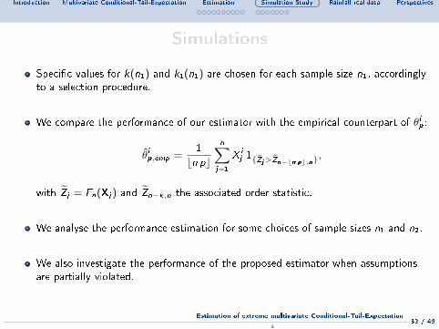
Speci�c values for k(n1) and k1(n1) are chosen for each sample size n1, accordinglyto a selection procedure.
We compare the performance of our estimator with the empirical counterpart of θip:
θ̂ip,emp =1
bn pc
n∑j=1
X ij 1{Z̃j>Z̃n−bn pc,n}
,
with Z̃j = Fn(Xj ) and Z̃n−k,n the associated order statistic.
We analyse the performance estimation for some choices of sample sizes n1 and n2.
We also investigate the performance of the proposed estimator when assumptionsare partially violated.
33 / 49Estimation of extreme multivariate Conditional-Tail-Expectation
N
Introduction Multivariate Conditional-Tail-Expectation Estimation Simulation Study Rainfall real data Perspectives Appendix
Copula 4.2.2 in Nelsen (1999)
Assume that (X 1,X 2) ∼ Copula 4.2.2 in Nelsen (1999).
Then φ(t) = (1− t)θ, for θ ∈ [1,+∞).
Assume now θ = 2. In this case R(X1,X2)(1, 1) = 0.59 and R(X1,Z)(1, 1) = 0.75.
Assume that γ1 = γ2 = 1/3 and ρ1 = ρ2 = −1.
↪→ We draw 500 samples from this distribution with sample sizes
n1 = n2 = 750, 250, 50
↪→ Based on each sample, we estimate θip(n1) for
p = 1/2 n1, p = 1/4 n1, p = 1/10 n1
34 / 49Estimation of extreme multivariate Conditional-Tail-Expectation
N

Introduction Multivariate Conditional-Tail-Expectation Estimation Simulation Study Rainfall real data Perspectives Appendix
n1 = 750, n2 = 750; p = 1/2 n1; p = 1/4 n1; p = 1/10 n1
0.0
0.5
1.0
1.5
2.0
2.5
Copula 4.2.2, with Pareto marginals gamma=1/3, n1=750, n2=750, k=400 k1=500
−3 −2 −1 0 1 2 3
−10
−5
05
10
Normal Q−Q Plot
Theoretical Quantiles
Sam
ple
Qua
ntile
s
0.0
0.5
1.0
1.5
2.0
2.5
Copula 4.2.2, with Pareto marginals gamma=1/3, n1=750, n2=750, k=400 k1=500
−3 −2 −1 0 1 2 3
−5
05
10
Normal Q−Q Plot
Theoretical QuantilesS
ampl
e Q
uant
iles
0.0
0.5
1.0
1.5
2.0
2.5
Copula 4.2.2, with Pareto marginals gamma=1/3, n1= 750, n2=750, k=400 k1=500
−3 −2 −1 0 1 2 3
−5
05
Normal Q−Q Plot
Theoretical Quantiles
Sam
ple
Qua
ntile
s
35 / 49Estimation of extreme multivariate Conditional-Tail-Expectation
N

Introduction Multivariate Conditional-Tail-Expectation Estimation Simulation Study Rainfall real data Perspectives Appendix
n1 = 250, n2 = 250; p = 1/2 n1; p = 1/4 n1; p = 1/10 n1
0.0
0.5
1.0
1.5
2.0
2.5
Copula 4.2.2, with Pareto marginals gamma=1/3, n1=250, n2=250, k=100 k1=150
−3 −2 −1 0 1 2 3
−6
−4
−2
02
46
Normal Q−Q Plot
Theoretical Quantiles
Sam
ple
Qua
ntile
s
0.0
0.5
1.0
1.5
2.0
2.5
Copula 4.2.2, with Pareto marginals gamma=1/3, n1=250, n2=250, k=100 k1=150
−3 −2 −1 0 1 2 3
−4
−2
02
46
8
Normal Q−Q Plot
Theoretical QuantilesS
ampl
e Q
uant
iles
0.0
0.5
1.0
1.5
2.0
2.5
Copula 4.2.2, with Pareto marginals gamma=1/3, n1=250, n2=250, k=100 k1=150
−3 −2 −1 0 1 2 3
−4
−2
02
46
Normal Q−Q Plot
Theoretical Quantiles
Sam
ple
Qua
ntile
s
36 / 49Estimation of extreme multivariate Conditional-Tail-Expectation
N

Introduction Multivariate Conditional-Tail-Expectation Estimation Simulation Study Rainfall real data Perspectives Appendix
n1 = 50, n2 = 50; p = 1/2 n1; p = 1/4 n1; p = 1/10 n1
0.0
0.5
1.0
1.5
2.0
2.5
Copula 4.2.2, with Pareto marginals gamma=1/3, n1=50, n2=50, k=30 k1=35
−3 −2 −1 0 1 2 3
−4
−2
02
4
Normal Q−Q Plot
Theoretical Quantiles
Sam
ple
Qua
ntile
s
0.0
0.5
1.0
1.5
2.0
2.5
Copula 4.2.2, with Pareto marginals gamma=1/3, n1=50, n2=50, k=30 k1=35
−3 −2 −1 0 1 2 3
−2
02
4
Normal Q−Q Plot
Theoretical QuantilesS
ampl
e Q
uant
iles
0.0
0.5
1.0
1.5
2.0
2.5
Copula 4.2.2, with Pareto marginals gamma=1/3, n1=50, n2=50, k=30 k1=35
−3 −2 −1 0 1 2 3
−2
−1
01
23
4Normal Q−Q Plot
Theoretical Quantiles
Sam
ple
Qua
ntile
s
37 / 49Estimation of extreme multivariate Conditional-Tail-Expectation
N

Introduction Multivariate Conditional-Tail-Expectation Estimation Simulation Study Rainfall real data Perspectives Appendix
n1 = 750, n2 = 750; p = 1/500 (left panel); p = 1/1000 (center panel); p = 1/1500 (right panel)
0.0
0.5
1.0
1.5
2.0
2.5
Copula 4.2.2, with Pareto marginals gamma=1/3, n1= 750, n2=750, k=400 k1=500
0.0
0.5
1.0
1.5
2.0
2.5
Copula 4.2.2, with Pareto marginals gamma=1/3, n1= 750, n2=750, k=400 k1=500
0.0
0.5
1.0
1.5
2.0
2.5
Copula 4.2.2, with Pareto marginals gamma=1/3, n1=750, n2=750, k=400 k1=500
0.0
0.5
1.0
1.5
2.0
2.5
Copula 4.2.2, with Pareto marginals gamma=1/3, n=1500, Empirical estimator
0.0
0.5
1.0
1.5
2.0
2.5
Copula 4.2.2, with Pareto marginals gamma=1/3, n=1500, Empirical estimator
0.0
0.5
1.0
1.5
2.0
2.5
Copula 4.2.2, with Pareto marginals gamma=1/3, n=1500, Empirical estimator
Figure : Boxplots of ratios between estimates and true values using the extreme estimator θ̂ip(n1),n2(�rst
row) and using the empirical estimator θ̂ip,emp with n = n1 + n2 = 1500 observations (second row).
38 / 49Estimation of extreme multivariate Conditional-Tail-Expectation
N

Introduction Multivariate Conditional-Tail-Expectation Estimation Simulation Study Rainfall real data Perspectives Appendix
Some choices for n1 and n2
Figure : Boxplots of ratios of estimates and true values for risk level p = 1/12 n1, �xed n1 = 250 and
n2 ∈ [2, 800] (left panel); p = 1/10 n1, �xed n1 = 50 and n2 ∈ [2, 20] (right panel).
↪→ Auxiliary sequences k = k(n1) and k1 = k1(n1) of the estimation procedure are chosen for each
considered value of n1.
↪→ Remark that n2 can be chosen particularly much smaller than n1. Indeed, with n2 = 15 (resp.
n2 = 10), our estimator has only a very small bias. The part of the bias due to the discrepancy
between Z and Z̃ , reduces quickly with n2.
↪→ As expected, the variance in the estimation reduces with n1.
39 / 49Estimation of extreme multivariate Conditional-Tail-Expectation
N

Introduction Multivariate Conditional-Tail-Expectation Estimation Simulation Study Rainfall real data Perspectives Appendix
Some choices for n1 and n2
Estimation when our assumptions are partially violated0.
00.
51.
01.
52.
02.
5
Copula 4.2.2, with Pareto marginals gamma=1/2, n1= 750, n2=750, k=450 k1=500, p=1/(2 n1)
0.0
0.5
1.0
1.5
2.0
2.5
Copula 4.2.2, with Pareto marginals gamma=1/2, n1= 750, n2=750, k=450 k1=500, p=1/(4 n1)
0.0
0.5
1.0
1.5
2.0
2.5
Copula 4.2.2, with Pareto marginals gamma=1/2, n1= 750, n2=750, k=450 k1=500, p=1/(10 n1)
Figure : Copula 4.2.2 in Nelsen (1999) with parameter θ = 2 and Pareto marginals with γ1 = γ2 = 1/2.
Here n1 = 750, n2 = 750 and Monte-Carlo simulations M = 500. Left panel p = 1/2 n1; center panel
p = 1/4 n1; right panel p = 1/10 n1.
Here γ1 = γ2 = 1/2. This distribution partially violates the conditions of the CLT.
However, the estimator θ̂ip(n1),n2is still consistent.
40 / 49Estimation of extreme multivariate Conditional-Tail-Expectation
N

Introduction Multivariate Conditional-Tail-Expectation Estimation Simulation Study Rainfall real data Perspectives Appendix
Some choices for n1 and n2
Estimation when our assumptions are partially violated0
510
15
Independence copula with Pareto marginals gamma=1/4, n1= 750, n2=750, k=450 k1=500, p=1/n1
05
1015
Independence copula with Pareto marginals gamma=1/4, n1= 750, n2=750, k=450 k1=500, p=1/(2 n1)
05
1015
Independence copula with Pareto marginals gamma=1/4, n1= 750, n2=750, k=450 k1=500, p=1/(4 n1)
Figure : Independent copula and Pareto distributed marginals with γ1 = γ2 = 1/4. Here n1 = 750,
n2 = 750 and Monte-Carlo simulations M = 500. Left panel p = 1/n1; center panel p = 1/2 n1; right
panel p = 1/4 n1.
We remark that, in this independent case, the proposed EVT estimator θ̂ip(n1),n2
overestimates the theoretical multivariate Conditional-Tail-Expectation.
41 / 49Estimation of extreme multivariate Conditional-Tail-Expectation
N
Introduction Multivariate Conditional-Tail-Expectation Estimation Simulation Study Rainfall real data Perspectives Appendix
Application to Rainfall real data
Data-set was provided by the SIAVB (Syndicat Intercommunal pourl'Assainissement de la Vallée de la Bièvre, see http://www.siavb.fr/).
Monthly mean in mm of the rainfall measurements recorded in 3 di�erent stationsof the region Bièvre (South of Paris), from 2003 to 2013.
The length of the data-set is n = 125. We take in the following n1 = 63, n2 = 62,so that n = n1 + n2.
We apply our estimation procedure to estimate the 3−variate CTE, i.e.,θip = E[X i |Z > UZ (1− p)], where i = 1, 2, 3 and Z = F (X 1,X 2,X 3).
42 / 49Estimation of extreme multivariate Conditional-Tail-Expectation
N
Introduction Multivariate Conditional-Tail-Expectation Estimation Simulation Study Rainfall real data Perspectives Appendix
Rainfall real data
Station 1
0 20 40 60 80
2040
6080
020
4060
80
Station 2
20 40 60 80 0 20 40 60 80
020
4060
80
Station 3
0 10 20 30 40 50 60
0.2
0.4
0.6
0.8
1.0
1.2
k1H
ill e
stim
ator
for
gam
ma_
i
Station 1Station 2Station 3
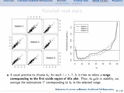
A usual practice to choose k1, for each i = 1, 2, 3, is then to select a rangecorresponding to the �rst stable region of this plot. Then, to gain in stability, weaverage the estimations γ̂ i corresponding to k1 in the selected range.
43 / 49Estimation of extreme multivariate Conditional-Tail-Expectation
N

Introduction Multivariate Conditional-Tail-Expectation Estimation Simulation Study Rainfall real data Perspectives Appendix
Rainfall real dataWe check R̂(X i ,Z̃)(1, 1) in term of the intermediate sequence k,
0 10 20 30 40 50
0.0
0.2
0.4
0.6
0.8
1.0
k
R̂(X1, Z~)(1, 1)R̂(X2, Z~)(1, 1)R̂(X3, Z~)(1, 1)
Now, using the values γ̂ i obtained before, we estimate the Multivariate CTE θip(n1)
and we plot the estimates against various values of the intermediate sequence k.
44 / 49Estimation of extreme multivariate Conditional-Tail-Expectation
N

Introduction Multivariate Conditional-Tail-Expectation Estimation Simulation Study Rainfall real data Perspectives Appendix
0 10 20 30 40 50 60
010
020
030
040
0Estimated CTEs, p = 1/(2 n1)
k
θ̂p
1
θ̂p
2
θ̂p
3
0 10 20 30 40 50 60
010
020
030
040
0
Estimated CTEs, p = 1/(4 n1)
k
θ̂p
1
θ̂p
2
θ̂p
3
0 10 20 30 40 50 60
010
020
030
040
0
Estimated CTEs, p = 1/(10 n1)
k
θ̂p
1
θ̂p
2
θ̂p
3
0 10 20 30 40 50 60
010
020
030
040
0
Estimated CTEs, p = 1/(20 n1)
k
θ̂p
1
θ̂p
2
θ̂p
3
0 10 20 30 40 50 60
010
020
030
040
0Estimated CTEs, p = 1/(30 n1)
k
θ̂p
1
θ̂p
2
θ̂p
3
0 10 20 30 40 50 60
010
020
030
040
0
Estimated CTEs, p = 1/(40 n1)
k
θ̂p
1
θ̂p
2
θ̂p
3
Figure : Estimated multivariate CTE (i.e., θ̂ip(n1),n2) against various values of the intermediate sequence
k, for i = 1, 2, 3 and for di�erent values of p. Here n1 = 63 and n2 = 62.
45 / 49Estimation of extreme multivariate Conditional-Tail-Expectation
N

Introduction Multivariate Conditional-Tail-Expectation Estimation Simulation Study Rainfall real data Perspectives Appendix
Station i γ̂ i θ̂ip=1/(2 n1),n2θ̂ip=1/(4 n1),n2
θ̂ip=1/(10 n1),n2θ̂ip=1/(20 n1),n2
θ̂ip=1/(30 n1),n2θ̂ip=1/(40 n1),n2
RP ≈ 10 years ≈ 21 years ≈ 52 years ≈ 105 years ≈ 157 years ≈ 210 years
1 0.259 65.579 78.524 99.637 119.305 132.563 142.854
2 0.363 108.782 139.964 195.307 251.292 291.212 323.325
3 0.359 105.331 135.133 187.845 240.994 278.805 309.179
Table : The estimates γ̂i are computed by taking the average for k1 in its �stability range�. The
estimates of the multivariate CTE are based on these values of γ̂i . We report the average of θ̂ip(n1),n2for
k ∈ [20, 45] and for di�erent values of p. Here n1 = 63 and n2 = 62.
↪→ These values θ̂ip(n1),n2represent the averaged monthly precipitations with di�erent
return periods.
↪→ We remark an important contribution of the second and third stations (i.e., X 2 andX 3) which strongly contribute to the multivariate stress scenario represented hereby the event {Z > UZ (1/p)}.
46 / 49Estimation of extreme multivariate Conditional-Tail-Expectation
N
Introduction Multivariate Conditional-Tail-Expectation Estimation Simulation Study Rainfall real data Perspectives Appendix
Some perspectives
Study the incidence of the form of K on the estimated variance of θip(n1).
Asymptotic independent case.
Avoid the decomposition the sample in n1 + n2 = n.
↪→ Z is a latent variable, which is not observed and has to beestimated. To prove the asymptotic properties of our plug-inestimator, we need to exploit the statistical properties of thecouples (Xi ,Z), where Z = F (X).
47 / 49Estimation of extreme multivariate Conditional-Tail-Expectation
N

Introduction Multivariate Conditional-Tail-Expectation Estimation Simulation Study Rainfall real data Perspectives Appendix
A short bibliography
Barbe, P., Genest, C., Ghoudi, K., and Rémillard, B. (1996). On Kendall's process. J.Multivariate Anal., 58(2):197-229.
Cai, J. J., Einmahl, J. H. J., de Haan, L., and Zhou, C. (2015). Estimation of the marginal
expected shortfall: the mean when a related variable is extreme. Journals of the RoyalStatistical Society, Series B, 77(2):417-442.
Chebana, F. and Ouarda, T. (2011). Multivariate quantiles in hydrological frequency
analysis. Environmetrics, 22(1):63-78.
Cousin, A. and Di Bernardino, E. (2014). On multivariate extensions of
Conditional-Tail-Expectation. Insurance: Mathematics and Economics, 55(0):272-282.
de Haan, L. and Huang, X. (1995). Large quantile estimation in a multivariate setting. J.Multivariate Anal., 53(2):247-263.
Di Bernardino, E. and Prieur, C. (2014). Estimation of multivariate
Conditional-Tail-Expectation using Kendall's process. Journal of Nonparametric Statistics,26(2):241-267.
Einmahl, J. H. J., de Haan, L., and Li, D. (2006). Weighted approximations of tail copula
processes with application to testing the bivariate extreme value condition. Ann. Statist.,34(4):1987-2014.
48 / 49Estimation of extreme multivariate Conditional-Tail-Expectation
N

Introduction Multivariate Conditional-Tail-Expectation Estimation Simulation Study Rainfall real data Perspectives Appendix
Thank you for your attention
49 / 49Estimation of extreme multivariate Conditional-Tail-Expectation
N

Introduction Multivariate Conditional-Tail-Expectation Estimation Simulation Study Rainfall real data Perspectives Appendix
We now introduce di�erent Gaussian processes that will be useful in the following tostate the asymptotic normality for the estimator of θip. Let i ∈ {1, . . . , d}. Let WR be azero mean Gaussian process on [0,∞]2 \ {(∞,∞)} with covariance structure
E[WR(Xi ,Z)
(x1, z1)WR(Xi ,Z)
(x2, z2)] = R(X i ,Z)(x1 ∧ x2, z1 ∧ z2).
Let
Θi = (γ i − 1)WR(Xi ,Z)
(∞, 1) +
(∫ ∞0
R(X i ,Z)(s, 1)ds−γi)−1 ∫ ∞
0
WR(Xi ,Z)
(s, 1) ds−γi
,
(1)and
Γi = γ i(−WR
(Xi ,Z)(1,∞) +
∫ ∞0
s−1WR(Xi ,Z)
(s,∞)ds
). (2)
49 / 49Estimation of extreme multivariate Conditional-Tail-Expectation
N