inhalt contents - billmann-web.de · the nonlinear relations are effective only at pid use. hat man...

Versuch 4 : Stetige Regelung Unit 4 : Steady Control

Inhalt1. Aufgabe..............................................................12. Größen, Einheiten, Definitionen.......................13. Grundlagen........................................................23.1. Der Universal-PID-Regler.................................23.2. Modellbildung der Regelstrecke........................43.3. Reglerentwurf mit Einstellregeln.......................73.4. Die J-BCASE Versuchsumgebung....................83.5. Der CDC-2000 Assistent...................................94. Versuchsvorbereitung.....................................104.1. Versuchsbedingungen....................................104.2. Versuchsprotokoll...........................................175. Versuchsdurchführung...................................185.1. Regelung mit konstanten Rücklauf-

Verhältnis........................................................185.2. Regelung mit veränderlichem Rücklauf-

Verhältnis........................................................195.3. Regelung mit Messstörungen.........................206. Versuchsauswertung.......................................21

ContentsScope......................................................................1Variables, units, definitions..................................1Basics.....................................................................2 The universal PID-controller..................................2 Modeling the Controlled System............................4 Controller design using tuning rules.......................7 The J-BCASE Test-Environment............................8 The CDC-2000 wizard...........................................9Exercise preparation...........................................10 Exercise conditions..............................................10 Exercise protocol.................................................17Exercise performance.........................................18 Control with constant reflux ratio

........................................................................18 Control with varying reflux ratio

........................................................................19 Control with measuring noise...............................20Exercise evaluation.............................................21

1. Aufgabe ScopeDie Aufgabe des Laborversuchs "Stetige Rege-

lung" besteht im Kennenlernen und praktischen Er-proben einfacher Regelungsvorgänge mit stetigen Regeleinrichtungen und ihre Einstellung. Die dabei gewählten Beispiele und Aufgabenstellungen wur-den bewusst einfach gehalten, um einen gewissen Grad von Vollständigkeit hierbei erzielen zu können.

The aim of the exercise 'steady control' is to get knowledge and experience in simple control mech-anisms by using steady controller units. The chosen examples and exercise targets have their focus on simplicity and as well on completeness.

2. Größen, Einheiten, Definitionen Variables, units, definitions

Dargestellte Größe Zeichenmark

Einheitunit variable usage

Anzahl der Simulationsschritte Nstep - number of simulation steps

Simulationsschrittweite Ts s simulation step size

Volumenstrom Q volume flowVolumenstrom (linearisiert) q [Q] volume flow (linearized)Füllstand H m filling levelRücklaufverhältnis r - reflux ratioAusfluss Koeffizient ε m / [Q]2 outflow coefficient

Querschnittsfläche Asp m2 cross-section area

Process Automation Laboratory – Steady Control 1 / 21 Prof.Dr.-Ing. L.Billmann (09.11.10)

3. Grundlagen BasicsIm Folgenden werden nochmals kurz die notwen-

digen Grundlagen zur Bearbeitung des Laborver-suchs dargestellt, wobei kein Anspruch auf Vollstän-digkeit erhoben werden kann. Bedingt durch den be-grenzten Umfang einer Versuchsbeschreibung muss teilweise auf eine vertiefte Darstellungen verzichtet werden, sofern sie nicht unbedingt zur Bearbeitung notwendig ist.Es sei hierfür auf die einschlägige Literatur oder maßgebliche Vorlesungsunterlagen verwiesen.

In the following we will summarize the basic top-ics which are necessary to workout this lab exercise. Due to the limited size of this lab documentation we disclaim deeper representations if it is not absolutely necessary for the handling.In case of further interest, please refer to other lec-ture notes or external literature on system control techniques.

3.1. Der Universal-PID-Regler The universal PID-controller

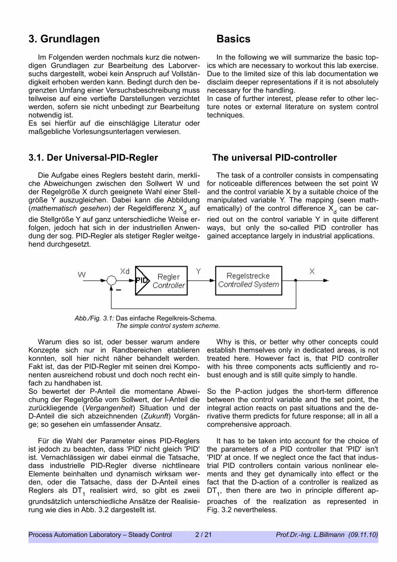
Die Aufgabe eines Reglers besteht darin, merkli-che Abweichungen zwischen den Sollwert W und der Regelgröße X durch geeignete Wahl einer Stell-größe Y auszugleichen. Dabei kann die Abbildung (mathematisch gesehen) der Regeldifferenz Xd auf die Stellgröße Y auf ganz unterschiedliche Weise er-folgen, jedoch hat sich in der industriellen Anwen-dung der sog. PID-Regler als stetiger Regler weitge-hend durchgesetzt.

The task of a controller consists in compensating for noticeable differences between the set point W and the control variable X by a suitable choice of the manipulated variable Y. The mapping (seen math-ematically) of the control difference Xd can be car-ried out on the control variable Y in quite different ways, but only the so-called PID controller has gained acceptance largely in industrial applications.

Warum dies so ist, oder besser warum andere Konzepte sich nur in Randbereichen etablieren konnten, soll hier nicht näher behandelt werden. Fakt ist, das der PID-Regler mit seinen drei Kompo-nenten ausreichend robust und doch noch recht ein-fach zu handhaben ist.

Why is this, or better why other concepts could establish themselves only in dedicated areas, is not treated here. However fact is, that PID controller with his three components acts sufficiently and ro-bust enough and is still quite simply to handle.

So bewertet der P-Anteil die momentane Abwei-chung der Regelgröße vom Sollwert, der I-Anteil die zurückliegende (Vergangenheit) Situation und der D-Anteil die sich abzeichnenden (Zukunft) Vorgän-ge; so gesehen ein umfassender Ansatz.

So the P-action judges the short-term difference between the control variable and the set point, the integral action reacts on past situations and the de-rivative therm predicts for future response; all in all a comprehensive approach.

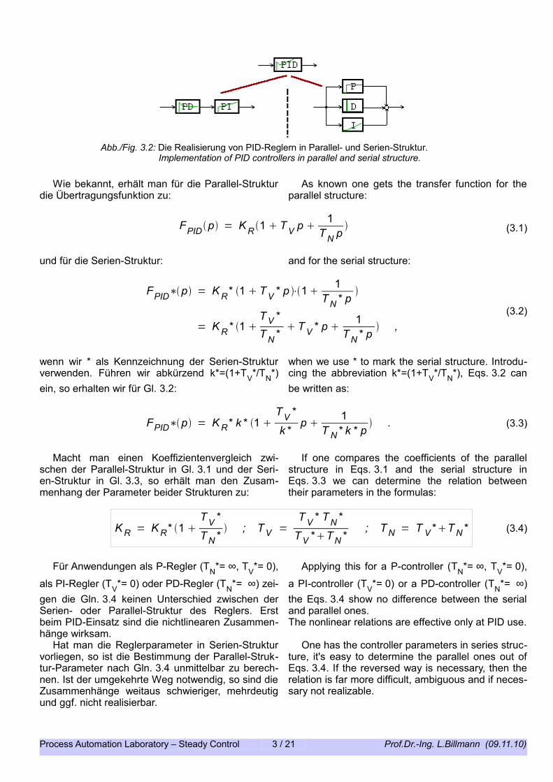
Für die Wahl der Parameter eines PID-Reglers ist jedoch zu beachten, dass 'PID' nicht gleich 'PID' ist. Vernachlässigen wir dabei einmal die Tatsache, dass industrielle PID-Regler diverse nichtlineare Elemente beinhalten und dynamisch wirksam wer-den, oder die Tatsache, dass der D-Anteil eines Reglers als DT1 realisiert wird, so gibt es zweii grundsätzlich unterschiedliche Ansätze der Realisie-rung wie dies in Abb. 3.2 dargestellt ist.

It has to be taken into account for the choice of the parameters of a PID controller that 'PID' isn't 'PID' at once. If we neglect once the fact that indus-trial PID controllers contain various nonlinear ele-ments and they get dynamically into effect or the fact that the D-action of a controller is realized as DT1, then there are two in principle different ap-proaches of the realization as represented in Fig. 3.2 nevertheless.


Abb./Fig. 3.1: Das einfache Regelkreis-Schema. The simple control system scheme.

Wie bekannt, erhält man für die Parallel-Struktur die Übertragungsfunktion zu:

As known one gets the transfer function for the parallel structure:

FPID p = K R 1 T V p 1

T N p (3.1)

und für die Serien-Struktur: and for the serial structure:

FPID∗p = K R* 1 T V * p ⋅11

T N * p

= K R * 1 T V *T N *

T V * p 1

T N * p ,

(3.2)

wenn wir * als Kennzeichnung der Serien-Struktur verwenden. Führen wir abkürzend k*=(1+TV*/TN*) ein, so erhalten wir für Gl. 3.2:

when we use * to mark the serial structure. Introdu-cing the abbreviation k*=(1+TV*/TN*), Eqs. 3.2 can be written as:

FPID∗p = K R* k * 1 T V *

k *p

1T N * k * p

. (3.3)

Macht man einen Koeffizientenvergleich zwi-schen der Parallel-Struktur in Gl. 3.1 und der Seri-en-Struktur in Gl. 3.3, so erhält man den Zusam-menhang der Parameter beider Strukturen zu:

If one compares the coefficients of the parallel structure in Eqs. 3.1 and the serial structure in Eqs. 3.3 we can determine the relation between their parameters in the formulas:

K R = K R* 1 T V *

T N * ; T V =

T V * T N *

T V *T N *; T N = T V *T N * (3.4)

Für Anwendungen als P-Regler (TN*= ∞, TV*= 0),

als PI-Regler (TV*= 0) oder PD-Regler (TN*= ∞) zei-gen die Gln. 3.4 keinen Unterschied zwischen der Serien- oder Parallel-Struktur des Reglers. Erst beim PID-Einsatz sind die nichtlinearen Zusammen-hänge wirksam.

Applying this for a P-controller (TN*= ∞, TV*= 0),

a PI-controller (TV*= 0) or a PD-controller (TN*= ∞) the Eqs. 3.4 show no difference between the serial and parallel ones.The nonlinear relations are effective only at PID use.

Hat man die Reglerparameter in Serien-Struktur vorliegen, so ist die Bestimmung der Parallel-Struk-tur-Parameter nach Gln. 3.4 unmittelbar zu berech-nen. Ist der umgekehrte Weg notwendig, so sind die Zusammenhänge weitaus schwieriger, mehrdeutig und ggf. nicht realisierbar.

One has the controller parameters in series struc-ture, it's easy to determine the parallel ones out of Eqs. 3.4. If the reversed way is necessary, then the relation is far more difficult, ambiguous and if neces-sary not realizable.


Abb./Fig. 3.2: Die Realisierung von PID-Reglern in Parallel- und Serien-Struktur. Implementation of PID controllers in parallel and serial structure.

3.2. Modellbildung der Regelstrecke Modeling the Controlled System

Bei der Ermittlung geeigneter Reglerparameter ist eine mehr oder weniger gute Kenntnis der zu re-gelnden Strecke (auch Prozess genannt) notwendig.

At the determination of suitable controller para-meters a more or less good knowledge of the con-trolled system (also called process) is necessary.

Betrachtet man sich typische industrielle Anwen-dungen, so findet man sehr häufig Regelstrecken mit Ausgleich (stabil), die nicht zu Schwingungen neigen (aperiodisch), d.h. ein ausgeprägtes Verzö-gerungsverhalten aufweisen. Man nennt diese Art auch Verzugs-Regelstrecken oder Verzögerungs-systeme.

Looking at typical industrial applications one can find very frequently controlled systems with com-pensation (stable), which don't tend to vibrations (aperiodic), i.e. show a distinctive delay behavior. One also mentions this type as delay controlled sys-tems or shorter delay systems.

Solche Strecken zu beschreiben, wird gern das Übergangsverhalten herangezogen, d.h. die Reakti-on des Ausgangs der Regelstrecke auf eine sprung-förmige Änderung am Eingang.

In case of describing such systems it's well usual to consult the transition behavior, i.e. the reaction of the output of the controlled system to a stepwise change to its input.

Zur Beschreibung dieses Verhaltens ist ein Mo-dell der Regelstrecke nötig, das man entweder durch theoretische Überlegungen (theoretische Mo-dellbildung) oder durch praktische Betriebserfahrun-gen bzw. eigens durchgeführte Versuche (experi-mentelle Modellbildung) ermitteln kann.

For the description of this behavior a model of the controlled system is necessary, which can be evalu-ated either by theoretical considerations (theoretical modeling) or by experimental test (experimental modeling) especially.

Die theoretische Modellbildung: The theoretical modeling:

Gehen wir einmal davon aus, dass als Ergebnis einer theoretischen Modellbildung das dynamische Verhalten der Regelstrecke durch eine normalerwei-se nichtlineare Differentialgleichung

Let's assume that the result of a theoretical mod-eling of the dynamic behavior of a controlled system is usually described by a nonlinear differential equa-tion

X t = F dX t dt

, d 2 X t dt2 , ⋯ , d n X t

dtn , Y t (3.5)

beschrieben werden kann, so erhält man aus Gl. 3.5 unter Weglassung aller zeitlichen Ableitungen die Arbeitspunktgleichung zu

then we get from Eqs. 3.5 by eliminating all temporal deviations the operating equation in the form

X 0 = F Y 0 (3.6)


Abb./Fig. 3.3: Das Übergangsverhalten der Regelstrecke. The transition response of the controlled system.

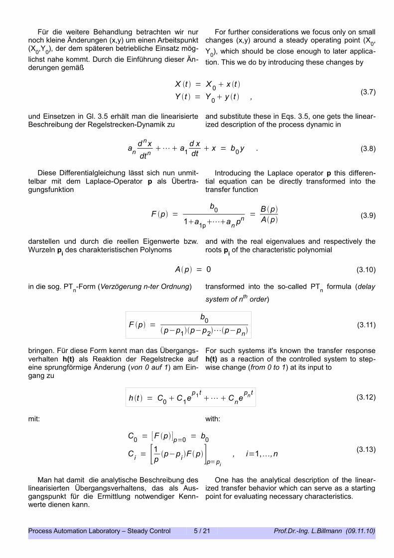
Für die weitere Behandlung betrachten wir nur noch kleine Änderungen (x,y) um einen Arbeitspunkt (X0,Y0), der dem späteren betriebliche Einsatz mög-lichst nahe kommt. Durch die Einführung dieser Än-derungen gemäß

For further considerations we focus only on small changes (x,y) around a steady operating point (X0, Y0), which should be close enough to later applica-tion. This we do by introducing these changes by

X t = X 0 x t Y t = Y 0 y t , (3.7)

und Einsetzen in Gl. 3.5 erhält man die linearisierte Beschreibung der Regelstrecken-Dynamik zu

and substitute these in Eqs. 3.5, one gets the linear-ized description of the process dynamic in

and nxdtn

⋯ a1d xdt

x = b0y . (3.8)

Diese Differentialgleichung lässt sich nun unmit-telbar mit dem Laplace-Operator p als Übertra-gungsfunktion

Introducing the Laplace operator p this differen-tial equation can be directly transformed into the transfer function

F p =b0

1a1p⋯an pn =B pAp (3.9)

darstellen und durch die reellen Eigenwerte bzw. Wurzeln pi des charakteristischen Polynoms

and with the real eigenvalues and respectively the roots pi of the characteristic polynomial

Ap = 0 (3.10)

in die sog. PTn-Form (Verzögerung n-ter Ordnung) transformed into the so-called PTn formula (delay

system of nth order)

F p =b0

p−p1p−p2⋯p−pn(3.11)

bringen. Für diese Form kennt man das Übergangs-verhalten h(t) als Reaktion der Regelstrecke auf eine sprungförmige Änderung (von 0 auf 1) am Ein-gang zu

For such systems it's known the transfer response h(t) as a reaction of the controlled system to step-wise change (from 0 to 1) at its input to

h t = C0 C1ep1 t

⋯ Cnepn t

(3.12)

mit: with:

C0 = [F p ]p=0 = b0

C i = [1p p−p i F p]p=pi

, i=1,,n (3.13)

Man hat damit die analytische Beschreibung des linearisierten Übergangsverhaltens, das als Aus-gangspunkt für die Ermittlung notwendiger Kenn-werte dienen kann.

One has the analytical description of the linear-ized transfer behavior which can serve as a starting point for evaluating necessary characteristics.


Die experimentelle Modellbildung: The experimental modeling:

Ist kein theoretisches Modell vorhanden, oder die Erstellung zu aufwendig, stellt man zur Bestimmung des Übergangsverhaltens die Bedingungen aus Abb. 3.3 experimentell nach, d.h. der Streckenein-gang wird durch eine möglichst große sprungförmi-ge Änderung von Y verstellt und die Reaktion X am Ausgang aufgezeichnet.

If there is no theoretical model available or the construction is too effortful one puts the conditions of Fig. 3.3 into an experimental environment to re-cord the step response. This is done by a big step-wise change of Y if possible to get a significant reac-tion at the output.

Problematisch dabei ist die Festlegung von wel-chem Wert Yvor ausgegangen werden soll und auf welchen Wert Ynach sich der Eingang ändern soll. Yvor und Ynach bestimmen dabei zwei stationäre Be-triebspunkte, die dem späteren Einsatz möglichst nahe kommen sollten. Andererseits darf durch den Versuch keine unzulässige Situation in der Regel-strecke auftreten, wie etwaige Grenzüberschreitun-gen oder Überlastungen. Für die bessere Auswer-tung sollte zudem noch die Änderung (Ynach-Yvor) am Eingang möglichst groß sein.

Problems might occur in choosing the initial value Yvor before the step and the final value Ynach after-wards because they correspond to two different op-erating points which have to be close to later applic-ation. On the other hand their might arise restriction in invalid levels of the process reaction. So a com-promise must be found in valid test conditions, enough stimulation and representative results.

Hat man den Versuch erfolgreich durchgeführt, können in der nachfolgenden Auswertung die erfor-derlichen Kennwerte ermittelt werden.

After the successful completion of the experiment the characteristics needed for later design can be evaluated out of the recorded data.

Ist eine sprungförmige Verstellung am Eingang nicht möglich (z.B. bei langsamen Ventilen), so reicht eine genügend steile rampenförmige Verän-derung des Eingangs aus, sofern diese schnell ge-nug im Vergleich zur Dynamik der Regelstrecke er-folgen kann.Ist eine solch schnelle Verstellung nicht möglich oder das Streckenverhalten zu schnell, bleibt noch die Möglichkeit nach Abb. 3.4.

If a stepwise change at the input is not possible (e.g. for slow reacting valves) one can try to use a sufficient steep ramp whenever it's fast enough in comparison to the process dynamics.

In minor cases, where such an approach isn't ac-ceptable a specialized possibility is given, as indic-ated in Fig. 3.4.

Hier wird die Regelstrecke bewusst mit einer langsamen, rampenförmigen Verstellung des Ein-gangs Y angeregt und die Reaktion X am Ausgang aufgezeichnet. Man erhält daraus das genäherte Übergangsverhalten, indem die erste zeitliche Ablei-tung der Reaktion X berechnet wird, was bei mer-kenswert gestörten Messsignalen nicht zu empfeh-lenswert ist.

Within here the process is stimulated by a rather slow ramp signal Y at the input where the output X is recorded. To get the desired step response the first temporal derivate has to be calculated with respect to a small noise level on the measured signal. Oth-erwise results may vary too much for later use.

Diese Methode basiert allerdings auf der Annahme, dass die Regelstrecke sich annähernd linear verhält.

This method is based on the assumption that the controlled system behaves roughly linearly, though.

3.3. Reglerentwurf mit Einstellregeln Controller design using tuning rules


Abb./Fig. 3.4: Das Übergangsverhalten der Regelstrecke bei Anregung mit einer Rampe. The transition response of the controlled system for stimulation with a ramp signal.

Angesichts der Schwierigkeiten, eine geeignete Reglereinstellung für eine gegebene Regelstrecke (Prozess) zu ermitteln, gibt es viele Ansätze dies in mehr oder weniger aufwendiger Form durchzufüh-ren, mit leider auch mehr oder weniger zufrieden-stellenden Ergebnissen (Regelverhalten).

In view of the difficulties of finding a suitable con-troller setting for a given controlled system (process) there are many attempts with results (control re-sponse) that satisfying unfortunately more or less .

Wir wollen uns hier auf die gebräuchlichste Form beschränken, aus Kennwerten der Regelstrecke über bekannte Einstellregeln die gewünschte Reg-lereinstellung (Parameter) direkt zu ermitteln.

We want to confine ourselves here to the most common form to find the desired controller setting (parameter) out directly from characteristic values of the controlled system response by known rules.

Der klassische Weg führt über eine sog. Tu/Tg-Beschreibung des Übergangsverhaltens der Regel-strecke und deren Näherung durch die Kennwerte eines PT1-Tt Systems. Aus diesen Kennwerten (KP, Tu, Tt) geben unterschiedliche Autoren direkte For-meln zur Bestimmung der Reglerparameter an.

The classic way leads across a so-called Tu/Tg description of the transition behavior of the con-trolled system and its approximation by the charac-teristics of a PT1-Tt system. Different authors indic-ate direct formula from these values (Kp, Tu, Tt) to the setting of the controller parameters.


Abb./Fig. 3.5: Die unterschiedlichen Wege vom Prozess-Wissen zur Reglereinstellung. The different approaches from the process knowledge to the controller settings.

Als Hauptvertreter sind hier die Regeln nach Ziegler/Nichols (ZN) und Chien/Hrones/Reswick (CHR) zu nennen, die neben verschiedenen Regler-strukturen eines PID-Reglers (P, PD, PI, PID) auch nach dem Einsatz für Führungsregelung (häufig än-dernde Sollwerte) oder Festwertregelung (kaum veränderliche Sollwerte) unterscheiden.

As the two major players herein we've to mention the methods by Ziegler/Nichols (ZN) and Chien/Hrones/Reswick (CHR), who give a formula for different structures of a PID-controller (P, PD, PI, PID) for use in reference control (frequent changing set points) as well as in noise control (hardly changes in set point) applications.

Eine Sonderstellung nehmen die Einstellregeln nach Ziegler/Nichols ein, die nicht unbedingt das Übergangsverhalten der Regelstrecke benötigen, sondern durch einen Regelversuch mit einem P-Regler im geschlossenen Kreis bis an die Stabili-tätsgrenze sich heran tasten. Aus der dabei benutz-ten Verstärkung des Reglers Kkrit und der dabei auf-tretenden Periodendauer Tkrit der entstehenden Dauerschwingung werden unmittelbar Regeln zum Ermitteln der Reglerparameter angegeben.Wesentlicher Nachteil dieser Vorgehensweise ist darin zu sehen, dass für langsame Regelstrecken der Vorgang bis zum Erreichen der Dauerschwin-gung zu viel Zeit benötigt; also nur für schnelle Re-gelstrecken geeignet ist.

A special position take the setting rules by Zieg-ler/Nichols, which don't need the transition behavior of the controlled system absolutely, but base on a closed loop control test with a P-controller and is tuned close to the stability limit. Knowing the ampli-fication of the controller at stability limit Kkrit and the corresponding length of period Tkrit of the arising os-cillations, the rules show directly determination of the expected controller parameters.Main disadvantage of this method is the waste of time for slowly reacting controlled systems. So it's preferable used for fast systems.

Eine weitere Sonderstellung haben die Einstellre-geln nach Billmann, da diese gerade für langsame Regelstrecken nicht die vollständige Sprungantwort benötigen, sondern diese nur bis zu ihrem Wende-punkt. Aus den daraus bestimmbaren Kennwerten für Tu und Vmax (max. Anstiegsgeschwindigkeit) wer-den unmittelbar Regeln zur Einstellung angegeben (man spart hierdurch zwischen 60% und 75% der Versuchszeit ! ).

Another special position is taken by the setting rules of Billmann since they only need the step re-sponse of the controlled system up to its turning point. This results in much less experimental time ef-fort (about 60% to 75% less ! ) and is therefor pre-destined to slow systems. Evaluating the character-istics Tu and Vmax from the response, the rules dir-ectly determine the corresponding controller para-meters.

Anmerkung: Da man aus dem kürzeren Versuch nicht die Verstärkung der Regelstrecke ermitteln kann, ist für eine evtl. Simulation ein typischer Wert (1...7) anzuneh-men. An den Regelparametern ändert sich dadurch aber nichts.

Remark: Since one cannot find the amplification of the controlled system out from the shorter test, a typical value (1...7) has to be assumed for a possible simulation. At the rule parameters, however, nothing changes through this.

3.4. Die J-BCASE Versuchsumgebung The J-BCASE Test-Environment

Hierzu sei auf den Versuch „Schaltende Rege-lung“ verwiesen, in dem bereits die J-BASE Umge-bung, als auch deren Bedienung, ausführlich be-schrieben wurde.

For this, reference is given to the lab experiment “switching control”, where detailed descriptions of the J-BCASE environment as well as its operating interface can be found.


3.5. Der CDC-2000 Assistent The CDC-2000 wizard

Bei dem vorliegenden Control-Design-Center handelt es sich um ein Werkzeug zur Einstellung von Reglern für die zunächst einmal häufigste An-wendung der Verzugs-Regelstrecken.

The Control-Design-Center on hand is a tool for setting controller parameters for the most frequent type of application the delay controlled systems.

Da es sowohl für Regelstrecken unterschiedliche Beschreibungsformen gibt, als auch beim Regler-entwurf die verschiedensten Einstellregeln zur An-wendung kommen, werden die gebräuchlichsten Verfahren hier behandelt.

Since there are different description forms for controlled systems and also many different setting rules coming to application, the most common pro-cedures are treated here.

Die PID-Reglerstruktur ist für P, PI, PD oder PID wählbar und es wird auch auf die unterschiedliche Realisierung als serieller oder paralleler PID-Regler eingegangen.

Due to the possibilities of a PID-controller all structures like P, PI, PD or PID can be chosen and furthermore serial and parallel realization on PID is taken into account.

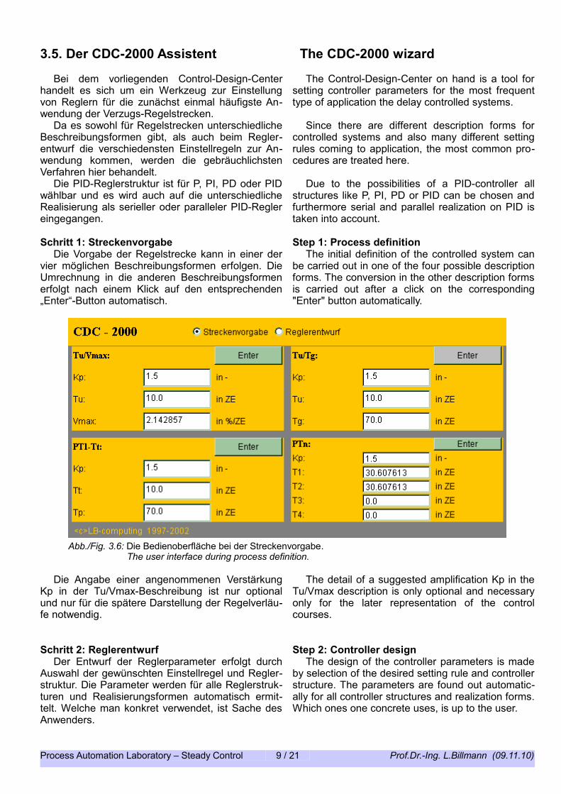
Schritt 1: Streckenvorgabe Step 1: Process definitionDie Vorgabe der Regelstrecke kann in einer der

vier möglichen Beschreibungsformen erfolgen. Die Umrechnung in die anderen Beschreibungsformen erfolgt nach einem Klick auf den entsprechenden „Enter“-Button automatisch.

The initial definition of the controlled system can be carried out in one of the four possible description forms. The conversion in the other description forms is carried out after a click on the corresponding "Enter" button automatically.

Die Angabe einer angenommenen Verstärkung Kp in der Tu/Vmax-Beschreibung ist nur optional und nur für die spätere Darstellung der Regelverläu-fe notwendig.

The detail of a suggested amplification Kp in the Tu/Vmax description is only optional and necessary only for the later representation of the control courses.

Schritt 2: Reglerentwurf Step 2: Controller designDer Entwurf der Reglerparameter erfolgt durch

Auswahl der gewünschten Einstellregel und Regler-struktur. Die Parameter werden für alle Reglerstruk-turen und Realisierungsformen automatisch ermit-telt. Welche man konkret verwendet, ist Sache des Anwenders.

The design of the controller parameters is made by selection of the desired setting rule and controller structure. The parameters are found out automatic-ally for all controller structures and realization forms. Which ones one concrete uses, is up to the user.


Abb./Fig. 3.6: Die Bedienoberfläche bei der Streckenvorgabe. The user interface during process definition.

4. Versuchsvorbereitung Exercise preparationBevor wir uns auf die einzelnen Versuche stür-

zen, seien hier zunächst die Versuchsgegebenhei-ten etwas näher beschrieben, insbesondere die Dy-namik der RegelstreckeDarüber hinaus wird ein Vorschlag beschrieben, wie die Versuchsergebnisse geeignet zu dokumentieren sind und auf was man dabei achten sollte.

Before we go into detail with the several test equipments, here the attempt conditions are some-what closer described, in particular the dynamic used for our experimental process.Beyond that a suggestion is described, how the test results can be documented suitably and hints are given on which one should be payed attention.

4.1. Versuchsbedingungen Exercise conditions

Schwerpunkte der Versuche sind die Regelung des Durchflusses und die Auslegung eines geeigne-ten PID-Reglers für eine Rührkessel-Anordnung, die sich durch nichtlineares Verhalten und eine Dynamik höherer Ordnung auszeichnet.Wir werden dazu zunächst eine vereinfachte Be-trachtung für einen einzelnen Rührkessel anstellen, um dann die Versuchsanordnung mit zwei gekoppel-ten Rührkesseln einfacher ableiten zu können.

Main emphases of the tests are the control of the flow and the design (parameter setting) of a suitable PID controller for a mixing boiler which stands out for nonlinear behavior and a dynamics of higher or-der.

At first we will make a simplified consideration for a single mixing boiler to this before we switch over o the more complex case of two coupled mixing boil-ers.

Der Einzel-Rührkessel: The single mixing boiler:

Betrachten wir zunächst die vereinfachte Anord-nung nach Abb. 4.1 eines Rührkessels mit zwei Pro-dukt-Zuflüssen (Qe1, Qe2) und einem Abfluss (Qa), der sich unmittelbar aus dem statischen Druck der Füllhöhe (H) bestimmt.

At first we view the simplified system of Fig. 4.1 of a single mixing boiler with the two product in-fluxes (Qe1, Qe2) and a drain (Qa) which immediately determines itself from the static pressure of the level (H).


Abb./Fig. 3.7: Die Bedienoberfläche beim Reglerentwurf. The user interface during controller design.

Wir beschränken uns hierbei lediglich auf die Be-handlung der Stoffströme (Volumenbilanz), d.h. Konzentration, chemische Reaktionen oder thermi-sche Effekte bleiben hier vereinfachend unbeachtet.

We confine ourselves to the treatment of the materi-al flows (volume balance), i.e. concentration merely, chemical reactions, or thermal effects remain here unnoticed for simplicity.

Beschränken wir uns auf die Volumenbilanz, so ist die zeitliche Änderung des im Behälters vorhan-denen Volumens Vsp durch die Differenz aus Zu- und Abfluss bestimmt.

We confine ourselves to the volume balance then the temporal change of the product volume Vsp in the boiler determines by the difference from influx and drain flow.

dV spdt

= Qe1 Qe2 − Qa(4.1)

mit der Querschnittsfläche Asp gilt dann with the cross-section area Asp is valid

V sp = Asp⋅H

und wir erhalten and we get

AspdHdt

= Qe1 Qe2 − Qa (4.2)

Da der Abfluss durch den statischen Druck bestimmt wird gilt

with the cross-section area Asp is valid

Qa ~ H

und damit der Zusammenhang and together with the relation

H = ⋅Qa2

mit dem Ausfluss Koeffizienten ε. Einsetzten in Gl. 4.2 liefert dann

with the outflow coefficient ε. Inserting this in Eqs. 4.2 leads finally to

AspdQa

2

dt Qa = Qe1 Qe2

(4.3)


Abb./Fig. 4.1: Anlagenskizze für einen Einzel-Rührkessel. Plant scheme of a single mixing boiler.

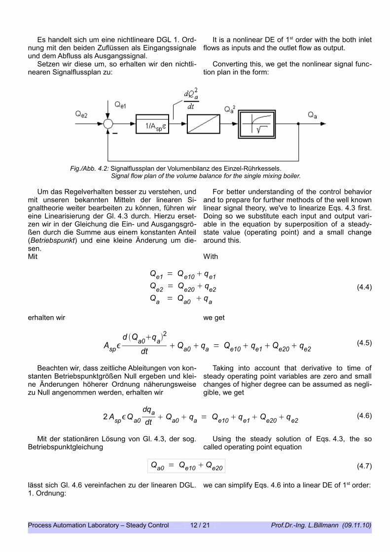
Es handelt sich um eine nichtlineare DGL 1. Ord-nung mit den beiden Zuflüssen als Eingangssignale und dem Abfluss als Ausgangssignal.

It is a nonlinear DE of 1st order with the both inlet flows as inputs and the outlet flow as output.

Setzen wir diese um, so erhalten wir den nichtli-nearen Signalflussplan zu:

Converting this, we get the nonlinear signal func-tion plan in the form:

Um das Regelverhalten besser zu verstehen, und mit unseren bekannten Mitteln der linearen Si-gnaltheorie weiter bearbeiten zu können, führen wir eine Linearisierung der Gl. 4.3 durch. Hierzu erset-zen wir in der Gleichung die Ein- und Ausgangsgrö-ßen durch die Summe aus einem konstanten Anteil (Betriebspunkt) und eine kleine Änderung um die-sen.

For better understanding of the control behavior and to prepare for further methods of the well known linear signal theory, we've to linearize Eqs. 4.3 first. Doing so we substitute each input and output vari-able in the equation by superposition of a steady-state value (operating point) and a small change around this.

Mit With

Qe1 = Qe10 qe1Qe2 = Qe20 qe2Qa = Qa0 qa

(4.4)

erhalten wir we get

Aspd Qa0qa

2

dt Qa0 qa = Qe10 qe1 Qe20 qe2

(4.5)

Beachten wir, dass zeitliche Ableitungen von kon-stanten Betriebspunktgrößen Null ergeben und klei-ne Änderungen höherer Ordnung näherungsweise zu Null angenommen werden, erhalten wir

Taking into account that derivative to time of steady operating point variables are zero and small changes of higher degree can be assumed as negli-gible, we get

2 AspQa0

dqadt

Qa0 qa = Qe10 qe1 Qe20 qe2(4.6)

Mit der stationären Lösung von Gl. 4.3, der sog. Betriebspunktgleichung

Using the steady solution of Eqs. 4.3, the so called operating point equation

Qa0 = Qe10 Qe20 (4.7)

lässt sich Gl. 4.6 vereinfachen zu der linearen DGL. 1. Ordnung:

we can simplify Eqs. 4.6 into a linear DE of 1st order:


Fig./Abb. 4.2: Signalflussplan der Volumenbilanz des Einzel-Rührkessels. Signal flow plan of the volume balance for the single mixing boiler.

2 AspQa0

dqadt

qa = qe1 qe2(4.8)

Es handelt sich demnach um ein sog. PT1-Ver-halten mit der Verstärkung 1 und einer Betrieb-spunkt abhängigen Zeitkonstanten, wie in dem li-nearen Signalflussplan dargestellt.

This represents a typical proportional delayed PT1 behavior with amplification of 1 and a operating point dependent time constant, as shown in the sig-nal flow plan below.

Vertiefung: Während Abb. 4.3 sich nur mit den sog. „Kleinsignalen“, also den kleinen Änderungen um einen Betriebspunkt, beschäftigt und Abb. 4.2 die „Großsignale „ in ihrem nichtlinearen Zusammenhang beschreibt, stellt die Darstellung in Abb. 4.4 eine Nähe-rung des Großsignal-Verhaltens durch Überlagerung einer einfachen Linearisierung mit den stationären Zu-sammenhängen dar.

In detail: While Fig. 4.3 only deals with the so called "small signals", namely the small changes around an operating point, and Fig. 4.2 describes the nonlinear interaction of the “large signals”, Fig. 4.4 represents an approximated behavior of the large signals using simple linearization and superposed steady state con-dition.

Der Doppel-Rührkessel mit Rückführung: The double mixing boiler with reflux:

Die eigentliche Versuchsanordnung, wie sie in Abb. 4.5 dargestellt ist, stellt eine Kaskade zweier Rührkessel dar, die mit einem wählbaren Rücklauf-verhältnis r ausgestattet ist.

The actually experimental arrangement, as rep-resented in Fig. 4.5, shows two mixing boilers in a cascade completed with an eligible reflux ratio r.


Abb./Fig. 4.3: Signalflussplan der linearisierten Volumenbilanz des Einzel-Rührkessels. Signal flow plan of the linearized volume balance for the single mixing boiler.

Abb./Fig. 4.4: Signalflussplan der linearisierten Volumenbilanz des Einzel-Rührkessels. Signal flow plan of the linearized volume balance for the single mixing boiler.

Aus der Anlagenskizze sind direkt die Zusam-menhänge für den stationären Zustand, die sog. Be-triebspunktgleichung,angebbar; wir erhalten

Out of the plant scheme we can directly determ-ine the steady-state relations, the so called operat-ing equations we get by

Qa10 = Qe0 r 0Qa20Qa20 = Qa10

= Qe0 r0 Qa201− r0Qa20 = Qe0

Qa20 =1

1−r0Qe0 , 0r01 !!

und schließlich den erwarteten Zusammenhang zu: and finally the expected relation to:

Qa0 = 1−r 0Qa20 = Qe0 (4.9)

Für das instationäre Verhalten könnten wir nun die Gl. 4.3 für beide Behälter anwenden und zu zwei gekoppelten nichtlinearen DGL's erster Ordnung ge-langen. Wir gehen hier aber den einfacheren Weg über den Signalflussplan nach Abb. 4.2, den wir in zweifacher Ausfertigung für die gegebene Anord-nung verschalten.

In order to get the non steady behavior we could apply Eqs. 4.3 for both boilers to get two nonlinear coupled DE's of first order. In contrast to this we go the more easy way using the signal flow plan of Fig. 4.2, which we use twice for our given plant scheme.


Abb./Fig. 4.5: Anlagenskizze für einen Doppel-Rührkessel mit Rückführung. Plant scheme of a double mixing boiler with reflux.

Gehen wir ganz analog dazu wiederum von Abb. 4.3 aus, so erhalten wir die linearisierte Be-schreibung des dynamischen Verhaltens der Volu-menströme.

Starting again out quite comparable to this out from Fig. 4.3, so we receive the linearized descrip-tion of the dynamic behavior of the volume flows in our plant.

Die beiden Zeitkonstanten bestimmen sich dann zu: Whereas the both time constants are determined by:

T 10 = 2 Asp11Qa10 = 2 Asp111

1−r 0Qe0

T 20 = 2 Asp22Qa20 = 2 Asp221

1−r 0Qe0

(4.10)

Da es sich bei dem Signalflussplan um zwei hin-tereinander geschaltete PT1-Systeme handelt, die aber über eine Mitkopplung (Rückführung hat positi-ves Vorzeichen) verschaltet sind, fassen wir die Ver-schaltung zunächst zusammen

Since the signal flow plan shows two PT1 sys-tems in series, which are interconnected by a posit-ive feedback, we've to combine this structure for fur-ther interpretations first into

qa2 p

qep=

11T 10 p

11T 20 p

1− 11T 10 p

11T 20 p

r 0

=1

1T 10p 1T 20 p − r 0

= 11−r 0 T 10T 20p T 10T 20p2

und damit mit and ahead with


Abb./Fig. 4.6: Signalflussplan der Volumenbilanz des Doppel-Rührkessels mit Rückführung. Signal flow plan of the volume balance for the double mixing boiler with reflux.

Abb./Fig. 4.7: Signalflussplan der linearisierten Volumenbilanz des Doppel-Rührkessels mit Rückführung. Signal flow plan of the linearized volume balance for the double mixing boiler with reflux.

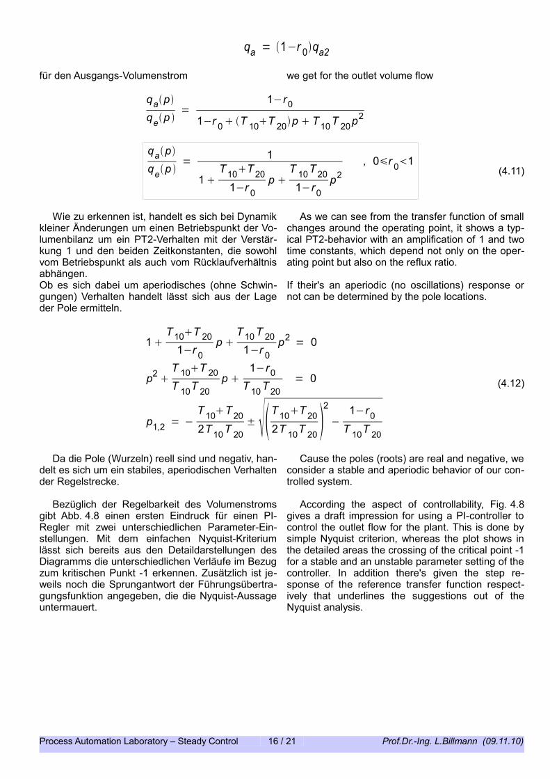
qa = 1−r 0qa2

für den Ausgangs-Volumenstrom we get for the outlet volume flow

qapqep

=1−r0

1−r 0 T 10T 20p T 10T 20p2

qapqep

= 1

1 T 10T 20

1−r 0p

T 10T 201−r0

p2, 0r 01

(4.11)

Wie zu erkennen ist, handelt es sich bei Dynamik kleiner Änderungen um einen Betriebspunkt der Vo-lumenbilanz um ein PT2-Verhalten mit der Verstär-kung 1 und den beiden Zeitkonstanten, die sowohl vom Betriebspunkt als auch vom Rücklaufverhältnis abhängen.

As we can see from the transfer function of small changes around the operating point, it shows a typ-ical PT2-behavior with an amplification of 1 and two time constants, which depend not only on the oper-ating point but also on the reflux ratio.

Ob es sich dabei um aperiodisches (ohne Schwin-gungen) Verhalten handelt lässt sich aus der Lage der Pole ermitteln.

If their's an aperiodic (no oscillations) response or not can be determined by the pole locations.

1 T 10T 20

1−r 0p

T 10T 201−r 0

p2 = 0

p2 T 10T 20T 10T 20

p 1−r0

T 10T 20= 0

p1,2 = −T 10T 202T 10T 20

± T 10T 202T 10T 20

2

−1−r0

T 10T 20

(4.12)

Da die Pole (Wurzeln) reell sind und negativ, han-delt es sich um ein stabiles, aperiodischen Verhalten der Regelstrecke.

Cause the poles (roots) are real and negative, we consider a stable and aperiodic behavior of our con-trolled system.

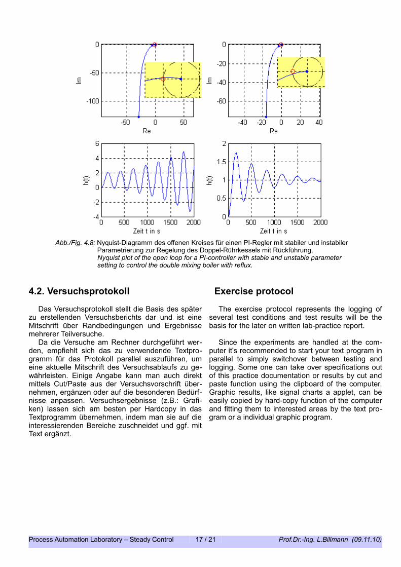
Bezüglich der Regelbarkeit des Volumenstroms gibt Abb. 4.8 einen ersten Eindruck für einen PI-Regler mit zwei unterschiedlichen Parameter-Ein-stellungen. Mit dem einfachen Nyquist-Kriterium lässt sich bereits aus den Detaildarstellungen des Diagramms die unterschiedlichen Verläufe im Bezug zum kritischen Punkt -1 erkennen. Zusätzlich ist je-weils noch die Sprungantwort der Führungsübertra-gungsfunktion angegeben, die die Nyquist-Aussage untermauert.

According the aspect of controllability, Fig. 4.8 gives a draft impression for using a PI-controller to control the outlet flow for the plant. This is done by simple Nyquist criterion, whereas the plot shows in the detailed areas the crossing of the critical point -1 for a stable and an unstable parameter setting of the controller. In addition there's given the step re-sponse of the reference transfer function respect-ively that underlines the suggestions out of the Nyquist analysis.


4.2. Versuchsprotokoll Exercise protocol

Das Versuchsprotokoll stellt die Basis des später zu erstellenden Versuchsberichts dar und ist eine Mitschrift über Randbedingungen und Ergebnisse mehrerer Teilversuche.

The exercise protocol represents the logging of several test conditions and test results will be the basis for the later on written lab-practice report.

Da die Versuche am Rechner durchgeführt wer-den, empfiehlt sich das zu verwendende Textpro-gramm für das Protokoll parallel auszuführen, um eine aktuelle Mitschrift des Versuchsablaufs zu ge-währleisten. Einige Angabe kann man auch direkt mittels Cut/Paste aus der Versuchsvorschrift über-nehmen, ergänzen oder auf die besonderen Bedürf-nisse anpassen. Versuchsergebnisse (z.B.: Grafi-ken) lassen sich am besten per Hardcopy in das Textprogramm übernehmen, indem man sie auf die interessierenden Bereiche zuschneidet und ggf. mit Text ergänzt.

Since the experiments are handled at the com-puter it's recommended to start your text program in parallel to simply switchover between testing and logging. Some one can take over specifications out of this practice documentation or results by cut and paste function using the clipboard of the computer. Graphic results, like signal charts a applet, can be easily copied by hard-copy function of the computer and fitting them to interested areas by the text pro-gram or a individual graphic program.


Abb./Fig. 4.8: Nyquist-Diagramm des offenen Kreises für einen PI-Regler mit stabiler und instabiler Parametrierung zur Regelung des Doppel-Rührkessels mit Rückführung. Nyquist plot of the open loop for a PI-controller with stable and unstable parameter setting to control the double mixing boiler with reflux.

5. Versuchsdurchführung Exercise performance

5.1. Regelung mit konstanten Rücklauf-Verhältnis

Control with constant reflux ratio

Gegeben ist die Versuchsanordnungen nach Abb. 4.5 des Doppel-Rührkessels mit Rückführung, dessen Ausgangs-Volumenstrom Qa mit einem steti-gen Regler geregelt werden soll. Als Stellgröße dient dazu der Zulauf-Volumenstrom Qe, während das Rücklaufverhältnis r (wenn Änderungen über-haupt) eine Störgröße darstellt.

Given is the test environment according Fig. 4.5 of a double mixing boiler with reflux whose outlet volume flow Qa is to be controlled by a steady PID controller. The inlet flow Qe is used as manipulated variable whereas the reflux ratio r (if changes at all) acts as a disturbance.

BCASE-D Setup: Zum Laden der Versuchsumgebung klicke man

im „Experiments“-Bereich zunächst auf J-BCA-SE, um die Framework-Seite zu starten. Von die-sem aus starte man das Simulationsprogramm BCASE-D und das Darstellungsprogramm BCA-SE-P.

BCASE-D Setup: To load the test environment just click on the J-

BCASE link in the “Experiments” section, to get the desired framework page. From there start the simulation program BCASE-D and the signal rep-resentation program BCASE-P.

Die benötigte Versuchsumgebung erhalten wir über den Menüpunkt „File-->Examples-->Double Mixing Boiler“. Wir erkennen den Regelkreis mit dem stetigen PID-Regler und die Regelstrecke (PROCESS) als unterlagertem Teilsystem (betre-ten mit Rechts-Klick, verlassen mit ESC).

We get the needed test environment via the menu “File-->Examples-->Double Mixing Boiler”. We recognize there the control system with the steady PID-controller and the controlled system (PROCESS) as an underlying subsystem (enter with right click, exit with ESC).

Weiterhin ist der SIGCHART-Block erkennbar, der die Signalverläufe über 400 Simulations-schritte darstellen kann, sowie der vcl4-Block, der die Signale in einer Datei vcl4.xml speichert, um sie dann genauer mit dem Darstellungsprogramm BCASE-P anzuzeigen.

Furthermore the SIGCHART block is recogniz-able which can represent the signal courses for 400 simulation steps as well as which the vcl4- block to store them additionally into the file vcl4.xml for detailed representation by the BCASE-P program afterwards.

Über den Menüpunkt „Sim/Debug-->Setup...“ stelle man die Schrittweite Ts=6s und die Anzahl der Simulationsschritte Nstep=400 ein.

Via the menu “Sim/Debug-->Setup...” we've to set the simulation step size Ts=6s and the num-ber of simulation steps Nstep=400.


J-BCASE

Versuchsläufe: Da der Regler sich im Hand-Betrieb befindet

(L_hand=1), ist der Regelkreis nicht geschlossen und der Regler gibt als Stellgröße Y den Hand-wert (Y_hand) aus. Aus einem Simulationslauf (Menü „Sim/Debug-->Simulate“) erkennt man, dass ein stationärer Betriebspunkt von Y=Qe0=Qa0=20% zu jedem Beginn einer Simula-tion vorliegen wird.

Experimental tests: Since the controller is in manual mode

(L_hand = 1) the control system isn't closed and the controller sets his output Y to the desired manual value (Y_hand). One recognizes from a simulation run (menu “Sim/Debug-- >Simulate") that stationary conditions Y=Qe0=Qa0=20% ap-pear at every initial of a simulation run.

Man nehme die Sprungantwort für einen Sprung von Y=20% auf Y=40% auf, indem man Yhand=40 einstellt und simuliert. Mit BCASE-P die Signale darstellen und mit der Wendetangente die Kenn-werte Kp (kennen wir mit 1), TU und TG grafisch ermittelt (BCASE-P auf maximale Fenstergröße, Lineal anlegen und mit Scan die Zeiten ermit-teln).

One takes the process response for a step of Y = 20% on Y = 40%, by adjusting Yhand = 40 and doing a simulation run. Representing the sig-nal courses by BCASE-P and using the turn tan-gent one can identify the characteristics KP (already known to 1), TU and TG in a graphical way (use BCASE-P with maximized window, place a ruler as turn tangent and measure time with scan facility).

Man wiederhole dies nochmals für Sprünge von 20% auf 60% und 20% auf 80% und vergleiche die ermittelten Kennwerte. Womit lassen sich ihre Unterschiede erklären ?

One repeats this for skips from 20% to 60% and 20% on 80% again and compares the determined identification values. How can her differences be explained ?

Man ermittle mit dem CDC-Assistenten die jewei-ligen (für alle drei Sprunghöhen) Parameter eines PID-Reglers (Xp, Tn, Tv) in Parallelstruktur mit den Einstellregeln nach Chien/Hrones/Reswick für Führungsregelung ohne Überschwingen und notiere auch die Angaben über die zu erwartende Anregelzeit (Tsettle) auf 1% und die Überschwing-weite (Xover).

One determines with the CDC-wizard the corres-ponding (all three step-sizes) parameters of a PID-controller (Xp, Tn, Tv) for parallel controller structure with the setting rules of Chien/Hrones/Reswick for reference control without overshooting and records the details on the expected rise time (Tsettle) on 1% and the about overshooting (Xover).

Man führe einen Regelversuch für einen Sollwert (Qa_soll) von 40% durch. Hierzu schalten man den Regler in Automatikbetrieb (L_hand=0), wähle den geeignetsten ermittelten Regler-Parameter-satz aus und geben diesen am Regler ein, bevor die Simulation erneut gestartet wird. Die Wahl des Parametersatzes ist zu begründen.

One performs a control experiment for a set point (Qa_soll) of 40%. For this the controller should work in automatic mode (L_hand=0) and a suit-able parameter setting has to be chosen before the simulation takes place again. The choice of the parameters should be explained.

Mit der gleichen Reglereinstellung wiederhole man dies für Sollwerte von 60% und 80% und vergleichen die Regel-Ergebnisse.Haben sich die Erwartungen bzgl. der Anregelzeit und der Überschwingweite bestätigt ?

With the same controller setting one repeats this for set points of 60% and 80% and compare the results.Where the expectations confirmed according the rise time and the overshooting ?

5.2. Regelung mit veränderlichem Rücklauf-Verhältnis

Control with varying reflux ratio

Mit der gleichen Versuchsanordnung soll nun der Einfluss sich ändernder Rücklauf-Verhältnisse unter-sucht werden. Da wir den Versuch über einen länge-ren Zeitraum durchführen wollen und dabei das Rücklauf-Verhältnis mehrfach ändern wollen, benut-zen wir den sog. Debug-Modus einer fortlaufenden Simulation.

With the same test order the influence of varying reflux ratios shall be examined now. Since we want to execute the simulation on a longer time period and change the reflux ratio repeatedly, we take ad-vantage of the so-called Debug mode of an ongoing simulation.


Versuchsläufe: Der Sollwert (Qa_soll) ist wieder auf 40% einzu-

stellen und der Debug-Mode über die Menüfunk-tion „SIM/Debug-->Init Debug Session“ zu star-ten. Durch Drücken der Tastenkombination Shift+A startet (fortsetzen) die Simulation und mit Shift+B hält sie wieder an.

Experimental tests: The set point (Qa_soll) has to be adjusted to 40%

and the Debug mode started via the menu func-tion " SIM/Debug -->Init Debug Session". By pushing the key combination Shift+A the simula-tion starts (continue) and it stops with pressing Shift+B again.

Man starte mit der Simulation und stoppe bei etwa 1000s, ändere r auf 0,4 und setze fort bis 2000s. Dort setze man r wieder auf 0,5 und setze fort bis 3000s, wo man schließlich r auf 0,6 setzt und bis 4000s simuliert. Um den Versuch nun or-dentlich zu beenden und die Daten auch in die Datei zu schreiben, beendet man den Debug-Mo-de mit der Menüfunktion „Sim/Debug-->Terminate Session“.

One starts with the simulation and stops at about 1000 s, changes r on 0.4 and puts away to 2000 s. There one puts r on 0.5 again and continues to 3000 s where one finally puts r on 0.6 and runs till 4000s. To conclude the test properly now and write the data also into the file one ends the Debug mode with the menu function “Sim/Debug-->Terminate Session".

Man stelle anschließend die Ergebnisse mit BCA-SE-P dar und interpretiere das Regelverhalten.

One then represents the results with BCASE-P and interprets the control response.

5.3. Regelung mit Messstörungen Control with measuring noise

Mit der gleichen Versuchsanordnung soll nun der Einfluss von Messstörungen untersucht werden, wo-bei wir wie unter Kapitel 5.1 die Simulation in einem Rutsch über 2400 s durchführen.

With the same test order the influence of meas-uring noise shall be examined now. Since we want to execute the simulation in one shot for 2400 s as used in chapter 5.1, we use not longer the debug mode.

Störungen können über den Parameter Knoise konfiguriert werden, der bislang auf dem Wert 0 ein-gestellt war. Der Wert von Knoise besagt, dass eine zufällige Messstörung mit maximal +/- Knoise % auf das Messsignal addiert wird.

Noise can be configured about the parameter Knoise which was adjusted on the value 0 till now. A value of Knoise means, that a measuring disturbance with maximum +/- Knoise % is added up on the measuring signal X (control variable).

Versuchsläufe: Mit einem Sollwert von 40% und einer Störung

von 0,5% (Knoise=0.5) führe man einen Regelver-such mit den bisherigen PID-Parametern durch und dokumentiere den Verlauf.

Experimental tests: With a set point of 40% and a noise of 0.5%

(Knoise = 0.5) one executes a control test with the previous PID parameters and documents the course.

Da die Störungen sich sehr stark auf das Stellsi-gnal Y auswirken und dies ein Stellglied zu stark beanspruchen würde, entnehme man dem CDC-Assistenten eine vergleichbare (siehe 5.1) Para-metereinstellung für einen PI-Regler. Mit diesem führe man den Versuch erneut durch und verglei-che die Ergebnisse des Regelverhaltens bzgl. des Stellglieds und der Regelgüte.

Since the noise has strongly affect to the manipu-lating variable Y and thus strongly burden the ac-tuator unit, one consult the CDC wizard again for a comparable parameter setting for a PI-control-ler. With this one executes the test once more and compares the results of the control response concerning the manipulating variable and the control accuracy.


6. Versuchsauswertung Exercise evaluationDie Versuchsauswertung ist eine kurz gefasste Zu-

sammenfassung der ermittelten Ergebnisse, Aus-wertung und Interpretation. Als Hilfestellung sind nachfolgend stichpunktartig die notwendigen In-halte Aufgeführt.

The exercise evaluation is a brief summary of the received results, evaluations and interpretations. As a support the necessary contents are listed below.

Zu 5.1::• Darstellung der drei Sprungantworten, ggf. in

einem Diagramm überlagert• Die ermittelten Kennwerte (KP,TU,TG) für die

drei Sprunghöhen und eine Erläuterung dazu

• Die ermittelten PID-Reglerparameter für die drei Sprunghöhen mit Erläuterung, welche Einstellung verwendet wird und warum

• Darstellung der Regelversuche für die drei Sollwerte, ggf. in einem Diagramm überlagert

• Die ermittelten Kenngrößen (Tsettle, Xover) für die drei Sollwerte und deren Erläuterung

Top 5.1:• representation of the three step responses, if

necessary in one diagram by overlapping.• the determined characteristics (KP,TU,TG) for

the three step-sizes and an adequate explana-tion

• the determined PID-controller parameters for the three step-sizes with explanation for the chosen overall setting.

• signal courses of the control test for all three set-points, if necessary in one diagram by overlapping.

• the determined characteristics (Tsettle, Xover) for the three set-points and some comments

Zu 5.2::• Darstellung des Regelverhaltens über 4000s

mit den verschiedenen Änderungen im Rück-laufverhältnis und eine kurze Interpretation dazu

Top 5.2:• representation of the control test over 4000s

with the different changes in the reflux ratio and a short explanation

Zu 5.3::• Darstellung des Regelverhaltens mit PID-Reg-

ler bei gestörtem Messsignal• Darstellung des Regelverhaltens mit PI-Regler

bei gestörtem Messsignal, Angabe der ver-wendeten PI-Parameter und Erläuterungen zum Vergleich der beiden Regelergebnisse bzgl. Stellsignal und Regelgüte.

Top 5.3:• representation of the control response of a

PID-controller using noise corrupted measure-ments

• representation of the control response of a PI-controller using noise corrupted measure-ments; documentation of the parameters used and comparing remarks towards the manipu-lating variable and the control accuracy

Abschließende Bemerkungen:• Zusammenfassende Anmerkungen, Interpre-

tationen und Bewertungen

Final remarks:Summarizing comments, interpretations and as-sessments


inhalt contents - billmann-web.de · the nonlinear relations are effective only at pid use. hat man...

Documents