information, liquidity, and dynamic limit order markets
TRANSCRIPT
Information, Liquidity, and
Dynamic Limit Order Markets∗
Roberto Ricco† Barbara Rindi‡ Duane J. Seppi§
May 16, 2018
Abstract
This paper describes price discovery and liquidity provision in a dynamic limit order market
with asymmetric information and non-Markovian learning. In particular, investors condition on
information in both the current limit order book and also, unlike in previous research, on the
prior trading history when deciding whether to provide or take liquidity. Numerical examples
show that the information content of the prior order history can be substantial. In addition,
the information content of arriving orders can be non-monotone in both the direction and
aggressiveness of arriving orders.
JEL classification: G10, G20, G24, D40
Keywords: Limit order markets, asymmetric information, liquidity, market microstructure
∗We thank Sandra Fortini, Thierry Foucault, Paolo Giacomazzi, Burton Hollifield, Phillip Illeditsch, Stefan Lewel-len, Marco Ottaviani, Tom Ruchti, and seminar participants at Carnegie Mellon University for helpful comments.We are grateful to Fabio Sist for his significant contribution to the computer code for our model.
†Bocconi University. Phone: +39-02-5836-2715. E-mail: [email protected]‡Bocconi University and IGIER. Phone: +39-02-5836-5328. E-mail: [email protected]§Tepper School of Business, Carnegie Mellon University. Phone: 412-268-2298. E-mail: [email protected]
The aggregation of private information and the dynamics of liquidity supply and demand are
closely intertwined in financial markets. In dealer markets, informed and uninformed investors
trade via market orders and, thus, take liquidity, while dealers provide liquidity and try to extract
information from the arriving order flow (e.g., as in Kyle (1985) and Glosten and Milgrom (1985)).
However, in limit order markets — the dominant form of securities market organization today
— the relation between who has information and who is trying to learn it and who supplies and
demands liquidity is not well understood theoretically.1 Recent empirical research highlights the
role of informed traders not only as liquidity takers but also as liquidity suppliers. O’Hara (2015)
argues that fast informed traders use market and limit orders interchangeably and often prefer limit
orders to marketable orders. Fleming, Mizrach, and Nguyen (2017) and Brogaard, Hendershott,
and Riordan (2016) find that limit orders play a significant empirical role in price discovery.2
Our paper presents the first rational expectations model of a dynamic limit order market with
asymmetric information and history-dependent Bayesian learning. In particular, learning is not
constrained to be Markovian. The model represents a trading day with market opening and closing
effects. Our model lets us investigate the information content of different types of market and limit
orders, the dynamics of who provides and demands liquidity, and the non-Markovian information
content of the trading history. In addition, we study how changes in the amount of adverse selection
— in terms of both asset-value volatility and the arrival probability of informed investors — affect
equilibrium trading strategies, liquidity, price discovery, and welfare. We have three main results:
• Increased adverse selection does not always worsen market liquidity as in Kyle (1985). Li-
quidity can improve if informed traders with better information trade more aggressively by
submitting more limit-orders at the inside quotes rather than using market orders.
1See Jain (2005) for a discussion of the prevalence of limit order markets. See Parlour and Seppi (2008) for asurvey of theoretical models of limit order markets. See Rindi (2008) for a model of informed traders as liquidityproviders.
2Gencay, Mahmoodzadeh, Rojcek, and Tseng (2016) investigate brief episodes of high-intensity/extreme behaviorof quotation process in the U.S. equity market (bursts in liquidity provision that happen several hundreds of timea day for actively traded stocks) and find that liquidity suppliers during these bursts significantly impact prices byposting limit orders.
1
• The relation between limit and market orders and their information content depends on the
size of private information shocks relative to the tick size. Indeed, the information content of
orders can even be opposite the order direction and aggressiveness.
• The learning dynamics are non-Markovian in that the order history has information in addi-
tion to the current state of the limit order book. In particular, the incremental information
content of arriving limit and market orders is history-dependent.
Dynamic limit order markets with uninformed investors are studied in a large literature. This
includes Foucault (1999), Parlour (1998), Foucault, Kadan, and Kandel (2005), and Goettler,
Parlour, and Rajan (2005). There is some previous theoretical research that allows informed traders
to supply liquidity. Kumar and Seppi (1994) is a static model in which optimizing informed and
uninformed investors use profiles of multiple limit and market orders to trade. Kaniel and Liu
(2006) extend the Glosten and Milgrom (1985) dealership market to allow informed traders to post
limit orders. Aıt-Sahalia and Saglam (2013) also allow informed traders to post limit orders, but
they do not allow them to choose between limit and market orders. Moreover, the limit orders
posted by their informed traders are always at the best bid and ask prices. Goettler, Parlour,
and Rajan (2009) allow informed and uninformed traders to post limit or market orders, but their
model is stationary and assumes Markovian learning. Rosu (2016b) studies a steady-state limit
order market equilibrium in continuous-time with Markovian learning and additional information-
processing restrictions. These last two papers are closest to ours. Our model differs from them
in two ways: First, they assume Markovian learning in order to study dynamic trading strategies
with order cancellation, whereas we simplify the strategy space (by not allowing dynamic order
cancellations and submissions) in order to investigate non-Markovian learning (i.e., our model has
a larger state space with full order histories). Second, we model a non-stationary trading day with
opening and closing effects. Market opens and closes are important daily events in the dynamics of
liquidity in financial markets. Bloomfield, O’Hara, and Saar (2005) show in an experimental asset
market setting that informed traders sometimes provide more liquidity than uninformed traders.
Our model provides equilibrium examples of liquidity provision by informed investors.
A growing literature investigates the relation between information and trading speed (e.g., Biais,
2

Foucault, and Moinas (2015); Foucault, Hombert, and Rosu (2016); and Rosu (2016a)). However,
these models assume Kyle or Glosten-Milgrom market structures and, thus, cannot consider the
roles of informed and uninformed traders as endogenous liquidity providers and demanders. We
argue that understanding price discovery dynamics in limit order markets is an essential precursor
to understanding speedbumps and cross-market competition given the real-world prevalence of limit
order markets.
1 Model
We consider a limit order market in which a risky asset is traded at five times tj ∈ {t1, t2, t3, t4, t5}
over a trading day. The fundamental value of the asset after time t5 at the end of the day is
v = v0 + ∆ =
v = v0 + δ with Pr(v) = 1
3
v0 with Pr(v0) = 13
v¯
= v0 − δ with Pr(v¯) = 1
3
(1)
where v0 is the ex ante expected asset value, and ∆ is a symmetrically distributed value shock. The
limit order market allows for trading through two types of orders: Limit orders are price-contingent
orders that are collected in a limit order book. Market orders are executed immediately at the best
available price in the limit order book. The limit order book has a price grid with four prices,
Pi ∈ {A2, A1, B1, B2}, two each on the ask and bid sides of the market. The tick size is equal to
κ > 0, and the ask prices are A1 = v0 + κ2 , A2 = v0 + κ, ; and by symmetry the bid prices are
B1 = v0 − κ2 , B2 = v0 − κ. Order execution in the limit order book follows time and price priority.
Investors arrive sequentially over time to trade in the market. At each time tj one investor
arrives. Investors are risk-neutral and asymmetrically informed. A trader is informed with prob-
ability α and uninformed with probability 1−α. Informed investors know the realized value shock
∆ perfectly. Uninformed investors do not know ∆, so they use Bayes’ Rule and their knowledge
of the equilibrium to learn about ∆ from the observable market dynamics over time. An investor
arriving at time tj may also have a personal private-value trading motive, which — we assume
3
for tractability — causes them to adjust their valuation of v0 to βtjv0 where the factor βtj may
be greater than or less than 1. Non-informational private-value motives include preference shocks,
hedging needs, and taxation. The absence of a non-informational trading motive would lead to the
Milgrom and Stokey (1982) no-trade result. The factor βtj at time tj is drawn from a truncated
normal distribution, Tr[N (µ, σ2)], with support over the interval [0, 2]. The mean is µ = 1, which
corresponds to a neutral private valuation. Traders with neutral private factors tend to provide
liquidity symmetrically on both the buy and sell sides of the market, while traders with extreme
private valuations provide one-sided liquidity or actively take liquidity. The parameter σ determines
the dispersion of a trader’s private-value factor βtj , as shown in Figure 1, and, thus, the probability
of large private gains-from-trade due to extreme investor private valuations.
The sequence of arriving investors is independently and identically distributed in terms of
whether they are informed or uninformed and in terms of their individual private-value factors
βtj . In one specification of our model, only uninformed investors have private valuations, while
in a second richer specification both informed and uninformed investors have private valuations.
A generic informed investor is denoted as I, where we denote the informed investor as Iv if the
value shock is positive (∆ = δ), as Iv¯
if the shock is negative (∆ = −δ), and as Iv0 if the shock is
zero (∆ = 0). Informed investors arriving at different times during the day all have the identical
asset-value information (i.e., there is only one realized ∆). Uninformed investors are denoted as U .
An investor arriving at time tj can take one of seven possible actions xtj : One possibility is
to submit a buy or sell market order MOAi,tj or MOBi,tj to buy or sell immediately at the best
available ask or bid respectively in the limit order book at time tj . A subscript i = 1 indicates that
the best standing quote at time tj is at the inside prices A1 or B1, and i = 2 means the best quote
is at the outside prices A2 or B2. Alternatively, the investor can submit one of four possible limit
orders LOAi and LOBi on the ask or bid side of the book, respectively. A subscript i = 1 denotes
an aggressive limit order posted at the inside quote, and i = 2 is a less aggressive limit order at the
outside quotes.3 Yet another alternative is to choose to do nothing (NT ).
For tractability, we make a few simplifying assumptions. Limit orders cannot be modified or
3For tractability, it is assumed that investors cannot post buy limit orders at A1 and sell limit orders at B1. Thisis one way in which the investor action space is simplified in our model.
4
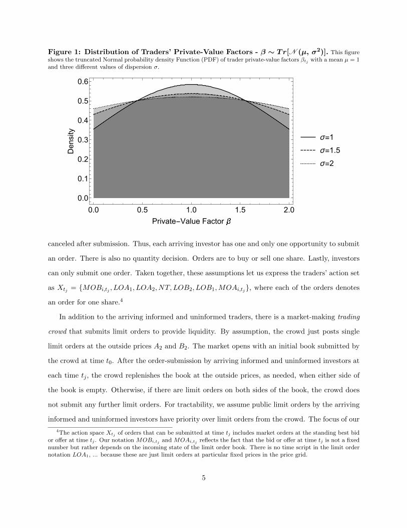
Figure 1: Distribution of Traders’ Private-Value Factors - β ∼ Tr[N (µ, σ2)]. This figureshows the truncated Normal probability density Function (PDF) of trader private-value factors βtj with a mean µ = 1and three different values of dispersion σ.
0.0 0.5 1.0 1.5 2.0
0.0
0.1
0.2
0.3
0.4
0.5
0.6
Private-Value Factor
Density
σ=1
σ=1.5
σ=2
canceled after submission. Thus, each arriving investor has one and only one opportunity to submit
an order. There is also no quantity decision. Orders are to buy or sell one share. Lastly, investors
can only submit one order. Taken together, these assumptions let us express the traders’ action set
as Xtj = {MOBi,tj , LOA1, LOA2, NT, LOB2, LOB1,MOAi,tj}, where each of the orders denotes
an order for one share.4
In addition to the arriving informed and uninformed traders, there is a market-making trading
crowd that submits limit orders to provide liquidity. By assumption, the crowd just posts single
limit orders at the outside prices A2 and B2. The market opens with an initial book submitted by
the crowd at time t0. After the order-submission by arriving informed and uninformed investors at
each time tj , the crowd replenishes the book at the outside prices, as needed, when either side of
the book is empty. Otherwise, if there are limit orders on both sides of the book, the crowd does
not submit any further limit orders. For tractability, we assume public limit orders by the arriving
informed and uninformed investors have priority over limit orders from the crowd. The focus of our
4The action space Xtj of orders that can be submitted at time tj includes market orders at the standing best bidor offer at time tj . Our notation MOBi,tj and MOAi,tj reflects the fact that the bid or offer at time tj is not a fixednumber but rather depends on the incoming state of the limit order book. There is no time script in the limit ordernotation LOA1, ... because these are just limit orders at particular fixed prices in the price grid.
5
model is on market dynamics involving information and liquidity given the behavior of optimizing
informed and uninformed investors. The crowd is simply a modeling device to insure it is always
possible for arriving investors to trade with market orders if they so choose.
Market dynamics over the trading day are intentionally non-stationary in our model in order
to capture market opening and closing effects. When the market opens at t1, the only standing
limit orders in the book are those at prices A2 and B2 from the trading crowd.5 At the end of the
day all unexecuted limit orders are cancelled. The state of the limit order book at a generic time
tj during the day is
Ltj = [qA2tj, qA1tj, qB1tj, qB2tj
] (2)
where qAitj
and qBitj
indicate the total depths at prices Ai and Bi at time tj . The limit order book
changes over time due to the arrival of new limit orders (which augment the depth of the book)
and market orders (which remove depth from the book) from arriving informed and uninformed
investors and due to the submission of limit orders from the crowd. The resulting dynamics are:
Ltj = Ltj−1 +Qtj + Ctj j = 1, . . . , 5 (3)
5In practice, daily opening limit order books include uncancelled orders from the previous day and new limitorders from opening auctions. For simplicity, we abstract from these interesting features of markets.
6
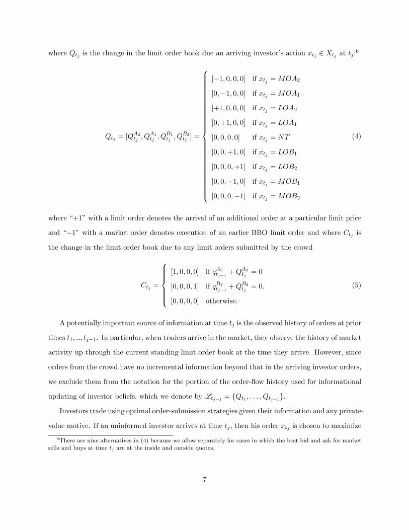
where Qtj is the change in the limit order book due an arriving investor’s action xtj ∈ Xtj at tj :6
Qtj = [QA2tj, QA1
tj, QB1
tj, QB2
tj] =
[−1, 0, 0, 0] if xtj = MOA2
[0,−1, 0, 0] if xtj = MOA1
[+1, 0, 0, 0] if xtj = LOA2
[0,+1, 0, 0] if xtj = LOA1
[0, 0, 0, 0] if xtj = NT
[0, 0,+1, 0] if xtj = LOB1
[0, 0, 0,+1] if xtj = LOB2
[0, 0,−1, 0] if xtj = MOB1
[0, 0, 0,−1] if xtj = MOB2
(4)
where “+1” with a limit order denotes the arrival of an additional order at a particular limit price
and “−1” with a market order denotes execution of an earlier BBO limit order and where Ctj is
the change in the limit order book due to any limit orders submitted by the crowd
Ctj =
[1, 0, 0, 0] if qA2
tj−1+QA2
tj= 0
[0, 0, 0, 1] if qB2tj−1
+QB2tj
= 0.
[0, 0, 0, 0] otherwise.
(5)
A potentially important source of information at time tj is the observed history of orders at prior
times t1, .., tj−1. In particular, when traders arrive in the market, they observe the history of market
activity up through the current standing limit order book at the time they arrive. However, since
orders from the crowd have no incremental information beyond that in the arriving investor orders,
we exclude them from the notation for the portion of the order-flow history used for informational
updating of investor beliefs, which we denote by Ltj−1 = {Qt1 , . . . , Qtj−1}.
Investors trade using optimal order-submission strategies given their information and any private-
value motive. If an uninformed investor arrives at time tj , then his order xtj is chosen to maximize
6There are nine alternatives in (4) because we allow separately for cases in which the best bid and ask for marketsells and buys at time tj are at the inside and outside quotes.
7
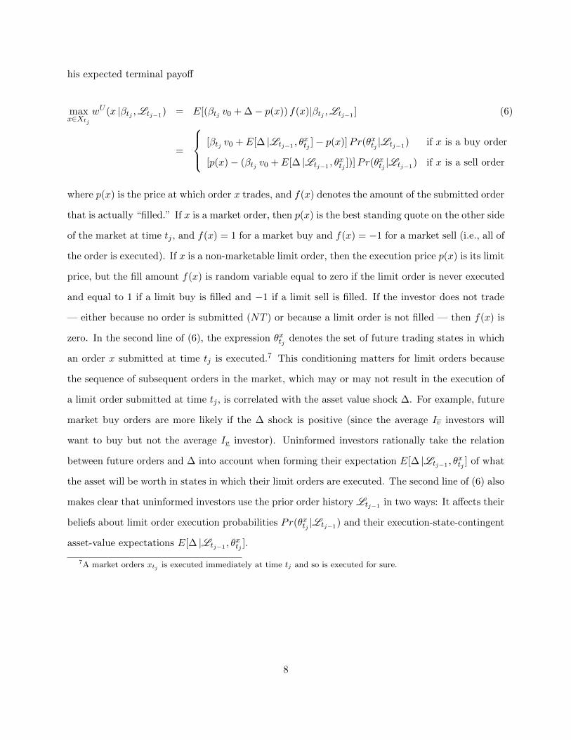
his expected terminal payoff
maxx∈Xtj
wU (x |βtj ,Ltj−1) = E[(βtj v0 + ∆− p(x)) f(x)|βtj ,Ltj−1 ] (6)
=
[βtj v0 + E[∆ |Ltj−1 , θxtj ]− p(x)]Pr(θxtj |Ltj−1) if x is a buy order
[p(x)− (βtj v0 + E[∆ |Ltj−1 , θxtj ])]Pr(θ
xtj |Ltj−1) if x is a sell order
where p(x) is the price at which order x trades, and f(x) denotes the amount of the submitted order
that is actually “filled.” If x is a market order, then p(x) is the best standing quote on the other side
of the market at time tj , and f(x) = 1 for a market buy and f(x) = −1 for a market sell (i.e., all of
the order is executed). If x is a non-marketable limit order, then the execution price p(x) is its limit
price, but the fill amount f(x) is random variable equal to zero if the limit order is never executed
and equal to 1 if a limit buy is filled and −1 if a limit sell is filled. If the investor does not trade
— either because no order is submitted (NT ) or because a limit order is not filled — then f(x) is
zero. In the second line of (6), the expression θxtj denotes the set of future trading states in which
an order x submitted at time tj is executed.7 This conditioning matters for limit orders because
the sequence of subsequent orders in the market, which may or may not result in the execution of
a limit order submitted at time tj , is correlated with the asset value shock ∆. For example, future
market buy orders are more likely if the ∆ shock is positive (since the average Iv investors will
want to buy but not the average Iv investor). Uninformed investors rationally take the relation
between future orders and ∆ into account when forming their expectation E[∆ |Ltj−1 , θxtj ] of what
the asset will be worth in states in which their limit orders are executed. The second line of (6) also
makes clear that uninformed investors use the prior order history Ltj−1 in two ways: It affects their
beliefs about limit order execution probabilities Pr(θxtj |Ltj−1) and their execution-state-contingent
asset-value expectations E[∆ |Ltj−1 , θxtj ].
7A market orders xtj is executed immediately at time tj and so is executed for sure.
8
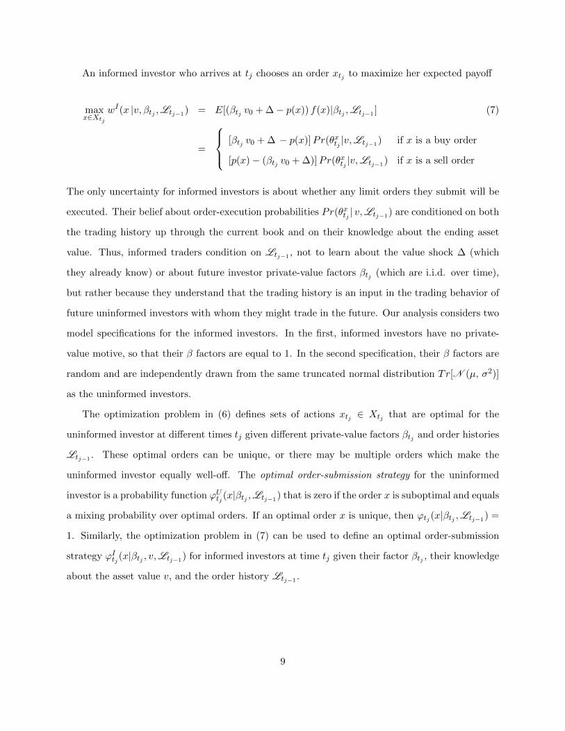
An informed investor who arrives at tj chooses an order xtj to maximize her expected payoff
maxx∈Xtj
wI(x |v, βtj ,Ltj−1) = E[(βtj v0 + ∆− p(x)) f(x)|βtj ,Ltj−1 ] (7)
=
[βtj v0 + ∆ − p(x)]Pr(θxtj |v,Ltj−1) if x is a buy order
[p(x)− (βtj v0 + ∆)]Pr(θxtj |v,Ltj−1) if x is a sell order
The only uncertainty for informed investors is about whether any limit orders they submit will be
executed. Their belief about order-execution probabilities Pr(θxtj | v,Ltj−1) are conditioned on both
the trading history up through the current book and on their knowledge about the ending asset
value. Thus, informed traders condition on Ltj−1 , not to learn about the value shock ∆ (which
they already know) or about future investor private-value factors βtj (which are i.i.d. over time),
but rather because they understand that the trading history is an input in the trading behavior of
future uninformed investors with whom they might trade in the future. Our analysis considers two
model specifications for the informed investors. In the first, informed investors have no private-
value motive, so that their β factors are equal to 1. In the second specification, their β factors are
random and are independently drawn from the same truncated normal distribution Tr[N (µ, σ2)]
as the uninformed investors.
The optimization problem in (6) defines sets of actions xtj ∈ Xtj that are optimal for the
uninformed investor at different times tj given different private-value factors βtj and order histories
Ltj−1 . These optimal orders can be unique, or there may be multiple orders which make the
uninformed investor equally well-off. The optimal order-submission strategy for the uninformed
investor is a probability function ϕUtj (x|βtj ,Ltj−1) that is zero if the order x is suboptimal and equals
a mixing probability over optimal orders. If an optimal order x is unique, then ϕtj (x|βtj ,Ltj−1) =
1. Similarly, the optimization problem in (7) can be used to define an optimal order-submission
strategy ϕItj (x|βtj , v,Ltj−1) for informed investors at time tj given their factor βtj , their knowledge
about the asset value v, and the order history Ltj−1 .
9
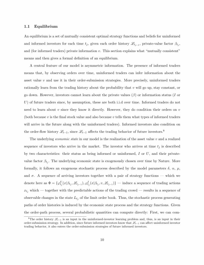
1.1 Equilibrium
An equilibrium is a set of mutually consistent optimal strategy functions and beliefs for uninformed
and informed investors for each time tj , given each order history Ltj−1 , private-value factor βtj ,
and (for informed traders) private information v. This section explains what “mutually consistent”
means and then gives a formal definition of an equilibrium.
A central feature of our model is asymmetric information. The presence of informed traders
means that, by observing orders over time, uninformed traders can infer information about the
asset value v and use it in their order-submission strategies. More precisely, uninformed traders
rationally learn from the trading history about the probability that v will go up, stay constant, or
go down. However, investors cannot learn about the private values (β) or information status (I or
U) of future traders since, by assumption, these are both i.i.d over time. Informed traders do not
need to learn about v since they know it directly. However, they do condition their orders on v
(both because v is the final stock value and also because v tells them what types of informed traders
will arrive in the future along with the uninformed traders). Informed investors also condition on
the order-flow history Lt−1, since Lt−1 affects the trading behavior of future investors.8
The underlying economic state in our model is the realization of the asset value v and a realized
sequence of investors who arrive in the market. The investor who arrives at time tj is described
by two characteristics: their status as being informed or uninformed, I or U , and their private-
value factor βtj . The underlying economic state is exogenously chosen over time by Nature. More
formally, it follows an exogenous stochastic process described by the model parameters δ, α, µ,
and σ. A sequence of arriving investors together with a pair of strategy functions — which we
denote here as Φ = {ϕUtj (x|βtj ,Ltj−1), ϕItj (x|βtj , v,Ltj−1)} — induce a sequence of trading actions
xtj which — together with the predictable actions of the trading crowd — results in a sequence of
observable changes in the state Ltj of the limit order book. Thus, the stochastic process generating
paths of order histories is induced by the economic state process and the strategy functions. Given
the order-path process, several probabilistic quantities can compute directly: First, we can com-
8The order history Lt−1 is an input in the uninformed-investor learning problem and, thus, is an input in theirorder-submission strategy. In addition, since future informed investors know that Lt−1 can affect uninformed investortrading behavior, it also enters the order-submission strategies of future informed investors.
10

pute the unconditional probabilities of different paths Pr(Ltj ) and the conditional probabilities
Pr(Qtj |Ltj−1) of particular order book changes Qtj due to arriving investors given a prior his-
tory Ltj−1 . Certain paths of orders are possible (i.e., have positive probability Pr(Ltj )) given the
strategy functions {ϕUtj (x|β,Ltj−1), ϕItj (x|β, v,Ltj−1)}, and certain paths of orders are not possible
(i.e., for which Pr(Ltj ) = 0). Second, the endogenous order-path process also determines the order-
execution probabilities Pr(θxtj | v,Ltj−1) and Pr(θxtj |Ltj−1) for informed and uninformed investors
for various orders x submitted at time tj . Computing each of these probabilities is simply a matter
of listing all of the possible underlying economic states, mechanically applying the order-submission
rules, identifying the relevant outcomes path-by-path, and then taking expectations across paths.
Let ` denote the set of all feasible histories {Ltj : j = 1, . . . , 4} of physically available orders
of lengths up to four trading periods. A four-period long history is the longest history a order-
submission strategy can depend on in our model. In this context, feasible paths are simply sequences
of actions from the action choice sets Xtj over time without regard to whether they are possible
in the sense that they occur with positive probability given the strategy functions Φ. Let ` in,Φ
denote the subset of all possible trading paths in ` that have positive probability, Pr(Ltj ) > 0,
given a pair of order strategies Φ. Let ` off,Φ denote the complementary set of trading paths that
are feasible but not possible given Φ. This notation will be useful when discussing “off equilibrium”
beliefs. In our analysis, strategy functions Φ are defined for all feasible paths in `. In particular,
this includes all of the possible paths in ` in,Φ given Φ and also the paths in ` off,Φ. As a result, the
probabilities Pr(Qtj |Ltj−1), Pr(θxtj | v,Ltj−1) and Pr(θxtj |Ltj−1) are always well-defined, because
the continuation trading process going forward — even after an unexpected order-arrival event (i.e.,
a path Ltj−1 ∈ ` off,Φ) — is still well-defined.
The stochastic process for order paths and its relation to the underlying economic state also
determine the uninformed-investor expectations E[v |Ltj−1 , θxtj ] of the terminal asset value given
the previous order history (Ltj−1) and conditional on future limit-order execution (θxtj ). These
expectations are determined as follows:
• Step 1: The conditional probabilities πvtj = Pr(v|Ltj ) of a particular final asset value v = v, v0
or v given a possible trading history Ltj ∈ ` in,Φ up through time tj is given by Bayes’ Rule.
11
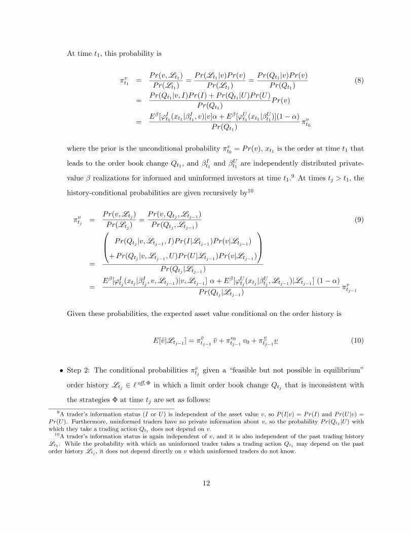
At time t1, this probability is
πvt1 =Pr(v,Lt1)
Pr(Lt1)=Pr(Lt1 |v)Pr(v)
Pr(Lt1)=Pr(Qt1 |v)Pr(v)
Pr(Qt1)(8)
=Pr(Qt1 |v, I)Pr(I) + Pr(Qt1 |U)Pr(U)
Pr(Qt1)Pr(v)
=Eβ[ϕIt1(xt1 |βIt1 , v)|v]α+ Eβ[ϕUt1(xt1 |βUt1)](1− α)
Pr(Qt1)πvt0
where the prior is the unconditional probability πvt0 = Pr(v), xt1 is the order at time t1 that
leads to the order book change Qt1 , and βIt1 and βUt1 are independently distributed private-
value β realizations for informed and uninformed investors at time t1.9 At times tj > t1, the
history-conditional probabilities are given recursively by10
πvtj =Pr(v,Ltj )
Pr(Ltj )=Pr(v,Qtj ,Ltj−1)
Pr(Qtj ,Ltj−1)(9)
=
Pr(Qtj |v,Ltj−1 , I)Pr(I|Ltj−1)Pr(v|Ltj−1)
+Pr(Qtj |v,Ltj−1 , U)Pr(U |Ltj−1)Pr(v|Ltj−1)
Pr(Qtj |Ltj−1)
=Eβ[ϕItj (xtj |β
Itj , v,Ltj−1)|v,Ltj−1 ] α+ Eβ[ϕUtj (xtj |β
Utj ,Ltj−1)|Ltj−1 ] (1− α)
Pr(Qtj |Ltj−1)πvtj−1
Given these probabilities, the expected asset value conditional on the order history is
E[v|Ltj−1 ] = πvtj−1v + πv0
tj−1v0 + π
vtj−1
v (10)
• Step 2: The conditional probabilities πvtj given a “feasible but not possible in equilibrium”
order history Ltj ∈ ` off,Φ in which a limit order book change Qtj that is inconsistent with
the strategies Φ at time tj are set as follows:
9A trader’s information status (I or U) is independent of the asset value v, so P (I|v) = Pr(I) and Pr(U |v) =Pr(U). Furthermore, uninformed traders have no private information about v, so the probability Pr(Qt1 |U) withwhich they take a trading action Qt1 does not depend on v.
10A trader’s information status is again independent of v, and it is also independent of the past trading historyLt1 . While the probability with which an uninformed trader takes a trading action Qt1 may depend on the pastorder history Ltj , it does not depend directly on v which uninformed traders do not know.
12
1. If the priors are fully revealing in that πvtj−1= 1 for some v, then πvtj = πvtj−1
for all v.
2. If the priors are not fully revealing at time tj , then πvtj = 0 for any v for which πvtj−1= 0
and the probabilities πvtj for the remaining v’s can be any non-negative numbers such
that πvtj + πv0tj
+ πvtj
= 1.
3. Thereafter, until any next unexpected trading event, the subsequent probabilities πvtj′
for j′ > j are updated according to Bayes’ Rule as in (9).
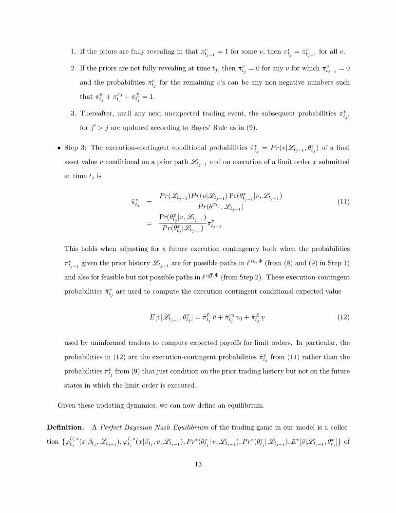
• Step 3: The execution-contingent conditional probabilities πvtj = Pr(v|Ltj−1 , θxtj ) of a final
asset value v conditional on a prior path Ltj−1 and on execution of a limit order x submitted
at time tj is
πvtj =Pr(Ltj−1)Pr(v|Ltj−1) Pr(θxtj−1
|v,Ltj−1)
Pr(θxtj ,Ltj−1)(11)
=Pr(θxtj |v,Ltj−1)
Pr(θxtj |Ltj−1)πvtj−1
This holds when adjusting for a future execution contingency both when the probabilities
πvtj−1given the prior history Ltj−1 are for possible paths in ` in,Φ (from (8) and (9) in Step 1)
and also for feasible but not possible paths in ` off,Φ (from Step 2). These execution-contingent
probabilities πvtj are used to compute the execution-contingent conditional expected value
E[v|Ltj−1 , θxtj ] = πvtj v + πv0
tjv0 + π
vtjv¯
(12)
used by uninformed traders to compute expected payoffs for limit orders. In particular, the
probabilities in (12) are the execution-contingent probabilities πvtj from (11) rather than the
probabilities πvtj from (9) that just condition on the prior trading history but not on the future
states in which the limit order is executed.
Given these updating dynamics, we can now define an equilibrium.
Definition. A Perfect Bayesian Nash Equilibrium of the trading game in our model is a collec-
tion {ϕU, ∗tj(x|βtj ,Ltj−1), ϕI, ∗tj (x|βtj , v,Ltj−1), P r∗(θxtj | v,Ltj−1), P r∗(θxtj |Ltj−1), E∗[v|Ltj−1 , θ
xtj ]} of
13

order-submission strategies, execution-probability functions, and execution-contingent conditional
expected asset-value functions such that:
• The equilibrium execution probabilities Pr∗(θxtj | v,Ltj−1) and Pr∗(θxtj |Ltj−1) are consistent
with the equilibrium order-submission strategies {ϕU, ∗tj+1(x|βtj+1 ,Ltj ), . . . , ϕ
U, ∗t5
(x|βt5 ,Lt4)}
and {ϕI, ∗tj+1(x|βtj+1 , v,Ltj ), . . . , ϕ
I, ∗t5
(x|βt5 , v,Lt4)} after time tj .
• The execution-contingent conditional expected asset values E∗[v|Ltj−1 , θxtj ]} agree with Bayesian
updating equations (8), (9), (11), and (12) in Steps 1 and 3 when the order x is consistent with
the equilibrium strategies ϕU, ∗tj(x|βtj ,Ltj−1) and ϕI, ∗tj (x|βtj , v,Ltj−1) at date tj and, when x is
an off-equilibrium action inconsistent with the equilibrium strategies, with the off-equilibrium
updating in Step 2.
• The positive-probability supports of the equilibrium strategy functions ϕU, ∗tj(x|βtj ,Ltj−1) and
ϕI, ∗tj (x|βtj , v,Ltj−1) (i.e., the orders with positive probability in equilibrium) are subsets of
the sets of optimal orders for uninformed and informed investors computed from their op-
timization problems (6) and (7) and the equilibrium execution probabilities and outcome-
contingent conditional asset-value expectation functions Pr∗(θxtj | v,Ltj−1), Pr∗(θxtj |Ltj−1),
and E∗[v|Ltj−1 , θxtj ].
Appendix A explains the algorithm used to compute the equilibria in our model. To help with
intuition, the next section walks through the order-submission and Bayesian updating mechanics
for a particular path in the extensive form of the trading game.
Our equilibrium concept differs from the Markov Perfect Bayesian Equilibrium used in Goettler
et al. (2009). Beliefs and strategies in our model are path-dependent; that is to say, traders use
Bayes Rule given the full prior order history when they arrive in the market. In contrast, Goettler
et al. (2009) restricts Bayesian updating to the current state of the limit order book and does not
allow for conditioning on the previous order history. Rosu (2016b) also assumes a Markov Perfect
Bayesian Equilibrium. The quantitative importance of the order history is considered when we
discuss our results in Section 2.
14
1.2 Illustration of order-submission mechanics and Bayesian updating
This section uses an excerpt of the extensive form of the trading game in our model to illustrate
order-submission and trading dynamics and the associated Bayesian updating process. The partic-
ular trading history path in Figure 2 is from the equilibrium for the model specification in which
informed and uninformed investors both have random private-value motives. The parameter values
are κ = 0.10, σ = 1.5, α = 0.8, and δ = 0.16, which is a market with a relatively high informed-
investor arrival probability and large value shocks. In this example, Nature has chosen an economic
state in which there is good news (v) about the asset, and the realized sequence of arriving traders
over time is {I, U, U, I, I}. At each node shown here, Figure 2 reports the total book Ltj of limit
orders from both arriving investors and the crowd. Trading starts at t1 with a book [1, 0, 0, 1] con-
sisting of no orders from informed and uninformed investors (since none have arrived yet) plus the
additional limit orders from the trading crowd (i.e., 1 each at the outside prices A2 and B2). For
simplicity, our discussion here only reports a few nodes of the trading game with their associated
equilibrium strategies. For example, we do not include NT at the end of t1, since, as we show later
in Section 2.2, NT is not an equilibrium action at t1 for these parameters.
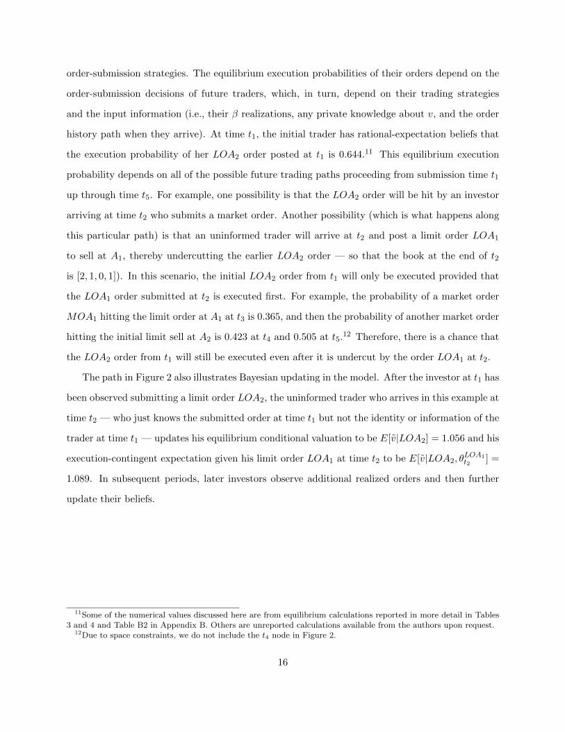
Investors in our equilibrium choose from a discrete number of possible orders given their re-
spective information and any private-value trading motives. Along the particular equilibrium path
considered here, the optimal strategies do not involve any randomization. Optimal orders are unique
given the inputs. However, orders are random due to randomness in the private factor β. Figure 2
shows below each order type at each time the probabilities with which the different orders are sub-
mitted by the trader who arrived. For example, if an informed trader Iv arrives at t1, she chooses
a limit order LOA2 to sell at A2 with probability 0.118. Each of these unique optimal orders is
associated with a different range of β types (for both informed and uninformed investors) and value
signals (for informed investors). Figure 3 illustrates where the order-submission probabilities come
from by superimposing the upper envelope of the expected payoffs for the different optimal orders
at time t1 on the truncated Normal β distribution. It shows how different β ranges correspond to
a discrete set of optimal orders delimited by the β thresholds. At each trading time, as the trading
game progresses along this path, traders submit orders (or do not trade) following their equilibrium
15
order-submission strategies. The equilibrium execution probabilities of their orders depend on the
order-submission decisions of future traders, which, in turn, depend on their trading strategies
and the input information (i.e., their β realizations, any private knowledge about v, and the order
history path when they arrive). At time t1, the initial trader has rational-expectation beliefs that
the execution probability of her LOA2 order posted at t1 is 0.644.11 This equilibrium execution
probability depends on all of the possible future trading paths proceeding from submission time t1
up through time t5. For example, one possibility is that the LOA2 order will be hit by an investor
arriving at time t2 who submits a market order. Another possibility (which is what happens along
this particular path) is that an uninformed trader will arrive at t2 and post a limit order LOA1
to sell at A1, thereby undercutting the earlier LOA2 order — so that the book at the end of t2
is [2, 1, 0, 1]). In this scenario, the initial LOA2 order from t1 will only be executed provided that
the LOA1 order submitted at t2 is executed first. For example, the probability of a market order
MOA1 hitting the limit order at A1 at t3 is 0.365, and then the probability of another market order
hitting the initial limit sell at A2 is 0.423 at t4 and 0.505 at t5.12 Therefore, there is a chance that
the LOA2 order from t1 will still be executed even after it is undercut by the order LOA1 at t2.
The path in Figure 2 also illustrates Bayesian updating in the model. After the investor at t1 has
been observed submitting a limit order LOA2, the uninformed trader who arrives in this example at
time t2 — who just knows the submitted order at time t1 but not the identity or information of the
trader at time t1 — updates his equilibrium conditional valuation to be E[v|LOA2] = 1.056 and his
execution-contingent expectation given his limit order LOA1 at time t2 to be E[v|LOA2, θLOA1t2
] =
1.089. In subsequent periods, later investors observe additional realized orders and then further
update their beliefs.
11Some of the numerical values discussed here are from equilibrium calculations reported in more detail in Tables3 and 4 and Table B2 in Appendix B. Others are unreported calculations available from the authors upon request.
12Due to space constraints, we do not include the t4 node in Figure 2.
16
Figure 2: Excerpt of the Extensive Form of the Trading Game. This figure shows one possibletrading path of the trading game with parameters α = 0.8, δ = 0.16, µ = 1, σ = 1.5, κ = 0.10, and 5 time periods.Before trading starts at time t1, the incoming book [1, 0, 0, 1] from time t0 consists of just the initial limit ordersfrom the crowd at A2 and B2. Nature selects a realized final value v = {v, v0, v} with probabilities { 1
3, 1
3, 1
3}. At
each trading period nature also selects an informed trader (I) with probability α and an uninformed trader (U) withprobability 1 − α. Arriving traders choose the optimal order at each period which may potentially include limitorders LOAi (LOBi) or market orders at the best ask, MOAi,t, or at the best bid, MOBi,t. Below each optimaltrading strategy we report in italics its equilibrium order-submission probability. Boldfaced equilibrium strategiesand associated states of the book (within double vertical bar) indicate the states of the book that we consider at eachnode of the chosen trading path.
A2 1A1 0B1 0B2 1
t0 v
t1
IMOA2 LOB1 LOB2 LOA2 LOA1 MOB2
0.256 0.282 0.030 0.118 0.314 0.0001 1 1 ‖ 2 ‖ 1 10 0 0 ‖ 0 ‖ 1 00 1 0 ‖ 0 ‖ 0 01 1 2 ‖ 1 ‖ 1 1
t2
I
...
α
UMOA2 LOB1 LOB2 LOA2 LOA1 MOB2
0.164 0.296 0.083 0.000 0.457 0.0001 2 2 3 ‖ 2 ‖ 20 0 0 0 ‖ 1 ‖ 00 1 0 0 ‖ 0 ‖ 01 1 2 1 ‖ 1 ‖ 1
t3
I
...
α
UMOA1 LOB1 LOB2 LOA2 LOA1 MOB2
0.365 0.000 0.219 0.000 0.058 0.358‖ 2 ‖ 2 2 3 2 2‖ 0 ‖ 1 1 1 2 1‖ 0 ‖ 1 0 0 0 0‖ 1 ‖ 1 2 1 1 1
t4I
...
t5
IMOA2 MOB2 NT0.505 0.345 0.150‖ 1 ‖ 2 2‖ 0 ‖ 0 0‖ 0 ‖ 0 0‖ 1 ‖ 1 1
α
U
...
1− α
α
U
...
1− α
1− α
1− α
α
U
...
1− α
13
v0
...
13
v...
13
Figure 3: β Distribution and Upper Envelope for Informed Investor Iv at time t1.This figure shows the private-value factor β ∼ Tr[N (µ, σ2)] distribution superimposed on the plot of the expectedpayoffs the informed investor Iv with good news at time t1 for each equilibrium order type MOA2, MOB2, LOA2,LOA1, LOB1, LOB2, NT , (solid colored lines) when the total book (including crowd limit orders) opens Lt0 = [10 0 1]. The dashed line shows the investor’s upper envelope for the optimal orders. The vertical black lines showthe β-thresholds at which two adjacent optimal strategies yield the same expected payoffs. For example LOA1 is theoptimal strategy for values of β between 0 and the first vertical black line; LOA2 is instead the optimal strategy forthe values of beta between the first and the second vertical lines; and so forth. The parameters are α = 0.8, δ = 0.16,µ = 1, σ = 1.5, and κ = 0.10.
MOA2LOB1LOB2LOA2LOA1
0.5 1.0 1.5 2.0β
-0.4
-0.2
0.2
0.4
0.6
MOA2
MOB2
LOA2
LOA1
LOB1
LOB2
NT
2 Results
Our analysis investigates how liquidity supply and demand decisions of informed and uninformed
traders and the learning process of uninformed traders affect market liquidity, price discovery, and
investor welfare. This section presents numerical results for our model. We first consider a model
specification in which only uninformed investors have a random private-value trading motive. In a
second specification, we generalize the analysis and show the robustness of our findings and extend
them. The tick size κ is fixed at 0.10, and the private-value dispersion σ is 1.5 throughout.
We focus on two time windows. The first is when the market opens at time t1. The second
is over the middle of the trading day from times t2 through t4. We look at these two windows
because our model is non-stationary over the trading day. Much like actual trading days, our
18
model has start-up effects at the beginning of the day and terminal horizon effects at the market
close. When the market opens at time t1, there are time-dependent incentives to provide, rather
than to take, liquidity: The incoming book is thin (with limit orders only from the crowd), and
there is the maximum time for future investors to arrive to hit limit orders from t1. There are also
time-dependent disincentives to post limit orders. Information asymmetries are maximal at time
t1, since there has been no learning from the trading process. Over the day, information is revealed
(lessening adverse selection costs), but the book can also become fuller (i.e., there is competition
in liquidity provision from earlier limit orders which have time priority at their respective limit
prices), and the remaining time for market orders to arrive and execute limit orders becomes
shorter. Comparing these two time windows shows how market dynamics change over the day. The
market close at t5 is also important, but trading then is straightforward. At the end of the day,
investors only submit market orders (or do not trade), because the execution probability for new
limit orders submitted at t5 is zero given our assumption that unfilled limit orders are canceled
once the market closes.
We use our model to investigate three questions: First, who provides and takes liquidity, and how
does the amount of adverse selection affect investor decisions to take and provide liquidity? Second,
how does market liquidity vary with different amounts of adverse selection? Third, how does the
information content of different types of orders depend on an order’s direction, aggressiveness, and
on the prior order history?
The amount of adverse selection can change in two ways: The proportion of informed traders can
change, and the magnitude of asset value shocks can change. We present comparative statics using
four different combinations of parameters with high and low informed-investor arrival probabilities
(α = 0.8 and 0.2) and high and low value-shock volatilities (δ = 0.16 and 0.02). We call markets
with δ = 0.02 low-volatility markets and markets with δ = 0.16 high-volatility markets, because the
arriving information is small relative to the tick size κ = 0.10 in the former parameterization and
larger relative to the tick size in the later. In high-volatility markets, the final asset value v given
good or bad news is beyond the outside quotes A2 or B2, and so even market orders at the outside
prices are profitable for informed traders. However, in low-volatility markets, v is always within
19
the inside quotes A1 and B1, and so market orders are never profitable for informed investors.
2.1 Uninformed traders with random private-value motives
In our first model specification, only uninformed traders have random private values. Informed
traders have fixed neutral private-value factors β = 1. Thus, as in Kyle (1985), there is a clear
differentiation between investors who speculate on private information and those who trade for
purely non-informational reasons. Unlike Kyle (1985), informed and uninformed investors can
trade using limit or market orders rather than being restricted to just market orders.
2.1.1 Trading strategies
We begin by investigating who supplies and takes liquidity and how these decisions change with
the amount of adverse selection. Table 1 reports results about trading early in the day at time t1
using a 2× 2 format. Each of the four cells corresponds to a different combination of parameters.
Comparing cells horizontally shows the effect of a change in the value-shock size δ while holding
the arrival probability α for informed traders fixed. Comparing cells vertically shows the effect of a
change in the informed-investor arrival probability while holding the value-shock size fixed. In each
cell corresponding to a set of parameters, there are four columns reporting conditional results for
informed investors with good news, neutral news, and bad news about the asset (Iv, Iv0 , Iv) and for
an uninformed investor (U) and a fifth column with the unconditional market results (Uncond). The
table reports the order-submission probabilities and several market-quality metrics. Specifically, we
report expected bid-ask spreads conditioning on the three informed-investor types E[Spread |Iv] and
on the uninformed trader E[Spread |U ], the unconditional expected market spread E[Spread], and
expected depths at the inside prices (A1 and B1) and total depths (A1+A2 and B1+B2) on each side
of the market. As we shall see, our results are symmetric for the directionally informed investors
Iv and Iv and on the buy and sell sides of the market. In addition, we report the probability-
weighted contributions to the different investors’ welfare (i.e., expected gains-from-trade) from
limit and market orders respectively, and their total expected welfare.13 Table B1 in Appendix B
13Let W (βt1) and W (v, βt1) denote the value functions when (6) and (7) are evaluated at time t1 using theoptimal strategies for the uninformed and informed investors respectively. The total welfare gain is E[W (βt1)] for
20
provides additional results about conditional and unconditional future execution probabilities for
the different orders (PEX(xt1)) and also the uninformed investor’s updated expected asset value
E[v|xt1 ] given different types of buy orders xt1 at time t1.
Table 2 shows average results for times t2 through t4 during the day using a similar 2×2 format.
The averages are across time and trading histories. Comparing results for time t1 with the trading
averages for t2 through t4 shows intraday changes in properties of the trading process. There is no
table for time t5, because only market orders are used at the market close.
Result 1 Changes in adverse selection due to the value-shock size δ affect trading strategies
differently than changes in the informed-investor arrival probability α.
The fact that different forms of adverse selection affect investors’ trading decisions differently
can been shown theoretically from first principles. Suppose the informed-investor arrival probability
α is close to zero. If the value-shock volatility δ is close to zero, then directionally informed investors
Iv and Iv with good or bad news never use market orders, since the final asset value v is always
between the inside bid and ask prices. However, if δ is sufficiently large, then investors with good
and bad news will start to use market orders given the guaranteed execution. Thus, the set of orders
used by directionally informed investors can change in these small α scenarios when δ changes. In
contrast, consider a market in which δ is close to zero. Now informed investors with good or bad
news never use market orders for any informed-investor arrival probability α. Thus, the set of
orders used by directionally informed investors never changes to include market orders in these
small δ scenarios when α changes.
the uninformed investor where the expectation is taken over βt1 and E[W (v, βt1)] for the informed investor wherethe expectation is taken over v and βt1 .
21
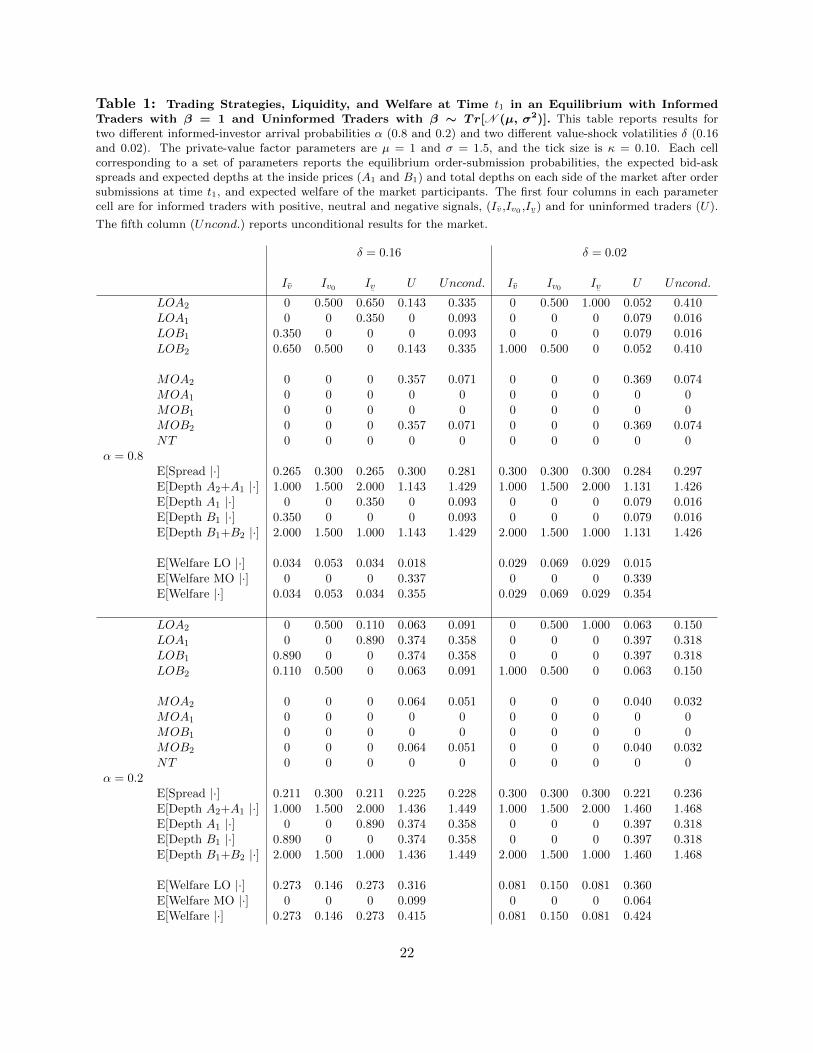
Table 1: Trading Strategies, Liquidity, and Welfare at Time t1 in an Equilibrium with InformedTraders with β = 1 and Uninformed Traders with β ∼ Tr[N (µ, σ2)]. This table reports results fortwo different informed-investor arrival probabilities α (0.8 and 0.2) and two different value-shock volatilities δ (0.16and 0.02). The private-value factor parameters are µ = 1 and σ = 1.5, and the tick size is κ = 0.10. Each cellcorresponding to a set of parameters reports the equilibrium order-submission probabilities, the expected bid-askspreads and expected depths at the inside prices (A1 and B1) and total depths on each side of the market after ordersubmissions at time t1, and expected welfare of the market participants. The first four columns in each parametercell are for informed traders with positive, neutral and negative signals, (Iv,Iv0 ,Iv
¯) and for uninformed traders (U).
The fifth column (Uncond.) reports unconditional results for the market.
δ = 0.16 δ = 0.02
Iv Iv0 Iv¯
U Uncond. Iv Iv0 Iv¯
U Uncond.
LOA2 0 0.500 0.650 0.143 0.335 0 0.500 1.000 0.052 0.410LOA1 0 0 0.350 0 0.093 0 0 0 0.079 0.016LOB1 0.350 0 0 0 0.093 0 0 0 0.079 0.016LOB2 0.650 0.500 0 0.143 0.335 1.000 0.500 0 0.052 0.410
MOA2 0 0 0 0.357 0.071 0 0 0 0.369 0.074MOA1 0 0 0 0 0 0 0 0 0 0MOB1 0 0 0 0 0 0 0 0 0 0MOB2 0 0 0 0.357 0.071 0 0 0 0.369 0.074NT 0 0 0 0 0 0 0 0 0 0
α = 0.8E[Spread |·] 0.265 0.300 0.265 0.300 0.281 0.300 0.300 0.300 0.284 0.297E[Depth A2+A1 |·] 1.000 1.500 2.000 1.143 1.429 1.000 1.500 2.000 1.131 1.426E[Depth A1 |·] 0 0 0.350 0 0.093 0 0 0 0.079 0.016E[Depth B1 |·] 0.350 0 0 0 0.093 0 0 0 0.079 0.016E[Depth B1+B2 |·] 2.000 1.500 1.000 1.143 1.429 2.000 1.500 1.000 1.131 1.426
E[Welfare LO |·] 0.034 0.053 0.034 0.018 0.029 0.069 0.029 0.015E[Welfare MO |·] 0 0 0 0.337 0 0 0 0.339E[Welfare |·] 0.034 0.053 0.034 0.355 0.029 0.069 0.029 0.354
LOA2 0 0.500 0.110 0.063 0.091 0 0.500 1.000 0.063 0.150LOA1 0 0 0.890 0.374 0.358 0 0 0 0.397 0.318LOB1 0.890 0 0 0.374 0.358 0 0 0 0.397 0.318LOB2 0.110 0.500 0 0.063 0.091 1.000 0.500 0 0.063 0.150
MOA2 0 0 0 0.064 0.051 0 0 0 0.040 0.032MOA1 0 0 0 0 0 0 0 0 0 0MOB1 0 0 0 0 0 0 0 0 0 0MOB2 0 0 0 0.064 0.051 0 0 0 0.040 0.032NT 0 0 0 0 0 0 0 0 0 0
α = 0.2E[Spread |·] 0.211 0.300 0.211 0.225 0.228 0.300 0.300 0.300 0.221 0.236E[Depth A2+A1 |·] 1.000 1.500 2.000 1.436 1.449 1.000 1.500 2.000 1.460 1.468E[Depth A1 |·] 0 0 0.890 0.374 0.358 0 0 0 0.397 0.318E[Depth B1 |·] 0.890 0 0 0.374 0.358 0 0 0 0.397 0.318E[Depth B1+B2 |·] 2.000 1.500 1.000 1.436 1.449 2.000 1.500 1.000 1.460 1.468
E[Welfare LO |·] 0.273 0.146 0.273 0.316 0.081 0.150 0.081 0.360E[Welfare MO |·] 0 0 0 0.099 0 0 0 0.064E[Welfare |·] 0.273 0.146 0.273 0.415 0.081 0.150 0.081 0.424
22
Table 2: Averages for Trading Strategies, Liquidity, and Welfare across Times t2 through t4 forInformed Traders with β = 1 and Uninformed Traders with β ∼ Tr[N (µ, σ2)]. This table reports resultsfor two different informed-investor arrival probabilities α (0.8 and 0.2) and for two different asset-value volatilitiesδ (0.16 and 0.02). The private-value factor parameters are µ = 1 and σ = 1.5, and the tick size is κ = 0.10. Eachcell corresponding to a set of parameters reports the equilibrium order-submission probabilities, the expected bid-askspreads and expected depths at the inside prices (A1 and B1) and total depths on each side of the market after ordersubmissions at times t2 through t4, and expected welfare for the market participants. The first four columns in eachparameter cell are for informed traders with positive, neutral and negative signals, (Iv,Iv0 ,Iv
¯) and for uninformed
traders (U). The fifth column (Uncond.) reports unconditional results for the market.
δ = 0.16 δ = 0.02
Iv Iv0 Iv¯
U Uncond. Iv Iv0 Iv¯
U Uncond.
LOA2 0 0.191 0.051 0.157 0.096 0.399 0.255 0.108 0.026 0.209LOA1 0 0.258 0.257 0.023 0.142 0.192 0.239 0.288 0.064 0.205LOB1 0.257 0.258 0 0.023 0.142 0.288 0.239 0.192 0.064 0.205LOB2 0.051 0.191 0 0.157 0.096 0.108 0.255 0.399 0.026 0.209
MOA2 0.493 0 0 0.286 0.189 0 0 0 0.347 0.069MOA1 0.001 0 0 0.031 0.006 0 0 0 0.058 0.012MOB1 0 0 0.001 0.031 0.006 0 0 0 0.058 0.012MOB2 0 0 0.493 0.286 0.189 0 0 0 0.347 0.069NT 0.198 0.061 0.198 0.007 0.124 0.013 0.010 0.013 0.011 0.012
α = 0.8E[Spread |·] 0.217 0.212 0.217 0.251 0.223 0.227 0.228 0.227 0.278 0.237E[Depth A2+A1 |·] 1.047 2.276 2.480 1.755 1.899 2.165 2.300 2.433 1.608 2.161E[Depth A1 |·] 0 0.438 0.829 0.243 0.387 0.226 0.362 0.506 0.131 0.318
E[Depth B1 |·] 0.829 0.438 0 0.243 0.387 0.506 0.362 0.226 0.131 0.318E[Depth B1+B2 |·] 2.480 2.276 1.047 1.755 1.899 2.433 2.300 2.165 1.608 2.161E[Welfare LO |·] 0.010 0.020 0.010 0.106 0.014 0.013 0.014 0.005E[Welfare MO |·] 0.009 0 0.009 0.298 0 0 0 0.354E[Welfare |·] 0.019 0.020 0.019 0.405 0.014 0.013 0.014 0.359
LOA2 0 0.358 0.508 0.102 0.139 0.375 0.389 0.443 0.093 0.155LOA1 0 0.122 0.258 0.056 0.070 0.044 0.096 0.116 0.066 0.070LOB1 0.258 0.122 0 0.056 0.070 0.116 0.096 0.044 0.066 0.070LOB2 0.508 0.358 0 0.102 0.139 0.443 0.389 0.375 0.093 0.155
MOA2 0.130 0 0 0.219 0.184 0 0 0 0.218 0.175MOA1 0.088 0 0 0.119 0.101 0 0 0 0.120 0.096MOB1 0 0 0.088 0.119 0.101 0 0 0 0.120 0.096MOB2 0 0 0.130 0.219 0.184 0 0 0 0.218 0.175NT 0.016 0.035 0.016 0.006 0.010 0.022 0.030 0.022 0.005 0.009
α = 0.2E[Spread |·] 0.205 0.190 0.205 0.280 0.264 0.221 0.217 0.221 0.300 0.284E[Depth A2+A1 |·] 1.305 2.089 2.512 1.583 1.660 1.932 2.091 2.257 1.576 1.680E[Depth A1 |·] 0.194 0.451 0.740 0.301 0.333 0.346 0.414 0.442 0.262 0.290E[Depth B1 |·] 0.740 0.451 0.194 0.301 0.333 0.442 0.414 0.346 0.262 0.290E[Depth B1+B2 |·] 2.512 2.089 1.305 1.583 1.660 2.257 2.091 1.932 1.576 1.680
E[Welfare LO |·] 0.119 0.086 0.119 0.052 0.060 0.064 0.060 0.050E[Welfare MO |·] 0.018 0 0.018 0.343 0 0 0 0.342E[Welfare |·] 0.137 0.086 0.137 0.394 0.060 0.064 0.060 0.392
23
Our numerical analysis illustrates this first result and also other facets of how adverse selection
affects investor trading strategies. Consider the directionally informed investors Iv and Iv with
good or bad news. First, hold the informed-investor arrival probability α fixed and increase the
amount of adverse selection by increasing the value-shock volatility δ. In a low-volatility market
in which value shocks ∆ are small relative to the tick size, informed traders with good and bad
news are unwilling to pay a large tick size to trade on their information and instead act as liquidity
providers who supply liquidity asymmetrically depending on the direction of their information.
This can be seen in Table 1 where in both of the two parameter cells on the right (with α = 0.8
and 0.2 and a small δ = 0.02) informed investors Iv and Iv at time t1 use limit orders at the outside
quotes A2 and B2 exclusively. In contrast, in a high-volatility market where value shocks are large
relative to the tick size, informed investors with good or bad news trade more aggressively. This
can be seen in the left two parameterization cells (with α = 0.8 and 0.2 and a large δ = 0.16)
where now informed investors Iv and Iv use limit orders at both the inside quotes A1 and B1 as
well at the outside quotes with positive probability at time t1. Now compare this to a change in
the amount of adverse selection due to a change in the informed-investor arrival probability α while
holding the value-shock size δ fixed. In this case, changing the amount of adverse selection does
not affect which orders informed investors with good and bad news use at time t1. This can be
seen by comparing the lower two parameter cells (with δ = 0.02 and 0.16 and a small α) with the
upper two parameter cells (with the same δs and a larger α).
The average order-submission probabilities at times t2 through t4 in Table 2 are qualitatively
similar to those for time t1. In low-volatility markets, informed investors Iv and Iv with good and
bad news tend to supply liquidity via limit orders following strategies in which order-submission
probabilities are somewhat skewed on the two sides of the market in the direction of their small
amount of private information. In contrast, in high-volatility markets, informed investors Iv and
Iv switch from providing liquidity on both sides of the market at times t2 to t4 to using a mix
of taking liquidity via market orders and supplying liquidity via limit orders on the same side of
the market as their information. Thus, once again, the trading strategies for informed investors Iv
and Iv are qualitatively similar holding δ fixed and changing α, but their trading strategies change
24
qualitatively when α is held fixed and δ is changed.
Next, consider informed investors I0 who know that the value shock ∆ is 0 and, thus, that
the unconditional prior v0 is correct. Tables 1 and 2 show that their liquidity provision trading
strategies are qualitatively the same at time t1 and on average over times t2 through t4. In constrast,
uninformed investors U become less willing to provide liquidity via limit orders at the inside quotes
as the adverse selection problem they face using limit orders worsens. Rather, they increasingly
take liquidity via market orders or supply liquidity by less aggressive limit orders at the outside
quotes. This reduction in liquidity provision at the inside quotes by uninformed investors happens
at time t1 (Table 1) and at times t2 through t4 (Table 2) both when the value shocks become larger
and when the arrival probability of informed investors increases.
Two equilibrium effects are noteworthy in this context. First, while the uninformed U investors
reduce their liquidity provision at the inside quotes as adverse selection increases, the I0 informed
investors increase their liquidity provision at the inside quotes. This is because I0 informed investors
have an advantage in liquidity provision over the uninformed U investors in that there is no adverse
selection risk for them. These results are qualitatively consistent with the intuition of Bloomfield,
O’Hara and Saar (BOS, 2005). Informed traders are more likely to use limit orders than market
orders when the value-shock volatility is low (and, thus, the profitability from trading on information
asymmetries is low), and to use market orders when the reverse is true.
Second, uninformed U investors are unwilling to use aggressive limit orders at the inside quotes
when the adverse selection risk is sufficiently high as in the upper left parametrization (α = 0.8 and
δ = 0.16). This explains the fact that informed investors Iv and Iv use aggressive limit orders at
the inside quotes with a higher probability at time t1 in the lower left parametrization (0.890 with
α = 0.2 and δ = 0.16) than in the upper left parameterization (0.350). At first glance this might
seems odd since competition from future informed investors (and the possibility of being undercut
by later limit orders) is greater when the informed-investor arrival probability is large (α = 0.8)
than when α is smaller. However, in equilibrium there is camouflage from the uninformed U
investors limit orders at the inside quotes in the lower left parametization, whereas limit orders
at the inside quotes are fully revealing in the upper left parametrization. As a result, Table B1
25

in Appendix B shows that the execution probabilities for the fully revealing limit orders at prices
which are revealed to be far from the asset’s actual value are much lower (0.078) relative to the
non-fully revealing limit orders (0.717).
2.1.2 Market quality
Market liquidity changes when the amount of adverse selection in a market changes. The standard
intuition, as in Kyle (1985), is that liquidity deteriorates given more adverse selection. For example,
Rosu (2016b) also finds worse liquidity (a wider bid-ask spread) given higher value volatility. How-
ever, we find that the standard intuition is not always true.
Result 2 Liquidity need not always deteriorate when adverse selection increases.
Markets can become more liquid given greater value-shock volatility if, given the tick size, high
volatility makes the value shock ∆ large relative the price grid. In addition, different measures of
market liquidity — expected spreads, inside depth, and total depth — can respond differently to
changes in adverse selection.
The impact of adverse selection on market liquidity follows directly from the trading strategy
effects discussed above. Two intuitions are useful in understanding our market liquidity results.
First, different investors affect liquidity differently. Informed traders with neutral news (Iv0) are
natural liquidity providers. Their impact on liquidity comes from whether they supply liquidity
at the inside (A1 and B1) or outside (A2 and B2) prices. In contrast, informed traders with
directional news (Iv and Iv) and uninformed traders (U) affect liquidity depending on whether
they opportunistically take or supply liquidity. Second, the most aggressive way to trade (both on
directional information and private values) is via market orders, which takes liquidity. However,
the next most aggressive way to trade is via limit orders at the inside prices. Thus, changes in
market conditions (i.e., δ and α) that make informed investors trade more aggressively (i.e., that
reduce their use of limit orders at the outside prices A2 and B2) can potentially improve liquidity
if their stronger trading interest migrates to aggressive limit orders at the inside quotes (A1 and
B1) rather than to market orders.
26
Our analysis shows that the standard intuition that adverse selection reduces market liquidity
depends on the relative magnitudes of asset-value shocks and the tick size. In Table 1, the expected
spread narrows at time t1 (markets become more liquid) when the value-shock volatility δ increases
(comparing parameterizations horizontally so that α is kept fixed). Liquidity improves in these
cases because the informed traders Iv and Iv submit limit orders at the inside quotes in these high-
volatility markets, whereas they only use limit orders at the outside quotes in low-volatility markets.
In constrast, the expected spread at time t1 widens when the informed-investor arrival probability
α increases holding the value-shock size δ constant, as predicted by the standard intuition. The
evidence against the standard intuition is even stronger in Table 2. At times t2 through t4, the
expected spread narrows both when information becomes more volatile (δ is larger) and when there
are more informed traders (when α is larger). The qualitative results for the expected depth at the
inside quotes goes in the same direction as the results for the expected spread. This is because both
results are driven by limit-order submissions at the inside quotes. The results for adverse selection
and total depth at both the inside and outside quotes are mixed. For example, total depth at time
t1 increases in Table 1 when value-shock volatility δ increases when the informed-investor arrival
probability α is high (comparing horizontally the two parametrizations on the top), but decreases
in δ when the informed α is low. In contrast, average total depth at times t2 through t4 in Table
2 is decreasing in the value-shock volatility (comparing parameterizations horizontally). This is
opposite the effect on the inside depth. Thus, different metrics for liquidity give mixed results.
The main result in this section is that the relation between adverse selection and market liquidity
is more subtle than the standard intuition. Increased adverse selection can improve liquidity.
The ability of investors to choose endogenously whether to supply or demand liquidity and at
what limit prices is what can overturn the standard intuition. Goettler et al. (2009) also have a
model specification with informed traders who have no private-value trading motive and uninformed
having only private-value motives. In their model, when volatility increases, informed traders reduce
their provision of liquidity and increase their demand of liquidity; with the opposite holding for
uninformed traders. Our results are more nuanced. Increased value-shock volatility is associated
with increased liquidity supply in some cases and with decreased liquidity in others. This is because
27

the tick size of the price grid constrains the prices at which liquidity can be supplied and demanded.
2.1.3 Information content of orders
Traders in real-world markets and empirical researchers are interested in the information content
of different types of arriving orders.14 A necessary condition for an order to be informative is
that informed investors use it. However, the magnitude of order informativeness is determined
by the mix of equilibrium probabilities with which both informed and uninformed traders use an
order. If uninformed traders use the same orders as informed investors, they add noise to the price
discovery process, and orders become less informative. In our model, the mix of information-based
and noise-based orders depends on the underlying proportion of informed investors α and and the
value-shock volatility δ.
We expect different market and limit orders to have different information content. A natural
conjecture is that the sign of the information revision associated with an order should agree with
the direction of the order (e.g., buy market and limit orders should lead to positive valuation
revisions). Another natural conjecture is that the magnitude of information revisions should be
greater for more aggressive orders. However, while the order-sign conjecture is true in our first
model specification, the order-aggressiveness conjecture does not always hold here.
Result 3 Order informativeness is not always increasing in the aggressiveness of an order.
This, at-first-glance surprising, result is another consequence of the impact of the tick size on
how informed investors trade on their information. As a result, the relative informativeness of
different market and limit orders can flip in high-volatility and low-volatility markets. The result is
immediate for market orders versus (less aggressive) limit orders in low-volatility markets in which
informed investors avoid market orders (see Table 1). However, this reversed ordering can also hold
for aggressive limit orders at the inside quotes (A1 and B1) versus less aggressive limit orders at
the outside quotes (A2 and B2).
14Fleming et al. (2017) extend the VAR estimation approach of Hasbrouck (1991) to estimate the price impacts oflimit orders as well as market orders. See also Brogaard et al. (2016).
28
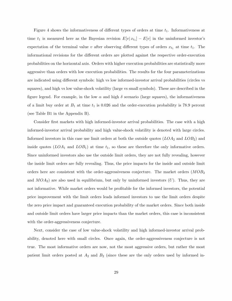
Figure 4 shows the informativeness of different types of orders at time t1. Informativeness at
time t1 is measured here as the Bayesian revision E[v|xt1 ] − E[v] in the uninformed investor’s
expectation of the terminal value v after observing different types of orders xt1 at time t1. The
informational revisions for the different orders are plotted against the respective order-execution
probabilities on the horizontal axis. Orders with higher execution probabilities are statistically more
aggressive than orders with low execution probabilities. The results for the four parameterizations
are indicated using different symbols: high vs low informed-investor arrival probabilities (circles vs
squares), and high vs low value-shock volatility (large vs small symbols). These are described in the
figure legend. For example, in the low α and high δ scenario (large squares), the informativeness
of a limit buy order at B1 at time t1 is 0.026 and the order-execution probability is 78.9 percent
(see Table B1 in the Appendix B).
Consider first markets with high informed-investor arrival probabilities. The case with a high
informed-investor arrival probability and high value-shock volatility is denoted with large circles.
Informed investors in this case use limit orders at both the outside quotes (LOA2 and LOB2) and
inside quotes (LOA1 and LOB1) at time t1, so these are therefore the only informative orders.
Since uninformed investors also use the outside limit orders, they are not fully revealing, however
the inside limit orders are fully revealing. Thus, the price impacts for the inside and outside limit
orders here are consistent with the order-aggressiveness conjecture. The market orders (MOB2
and MOA2) are also used in equilibrium, but only by uninformed investors (U). Thus, they are
not informative. While market orders would be profitable for the informed investors, the potential
price improvement with the limit orders leads informed investors to use the limit orders despite
the zero price impact and guaranteed execution probability of the market orders. Since both inside
and outside limit orders have larger price impacts than the market orders, this case is inconsistent
with the order-aggressiveness conjecture.
Next, consider the case of low value-shock volatility and high informed-investor arrival prob-
ability, denoted here with small circles. Once again, the order-aggressiveness conjecture is not
true. The most informative orders are now, not the most aggressive orders, but rather the most
patient limit orders posted at A2 and B2 (since these are the only orders used by informed in-
29
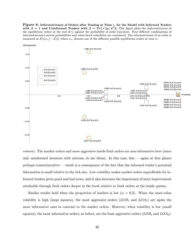
Figure 4: Informativeness of Orders after Trading at Time t1 for the Model with Informed Traderswith β = 1 and Uninformed Traders with β ∼ Tr[N (µ, σ2)]. This figure plots the Informativeness ofthe equilibrium orders at the end of t1 against the probability of order execution. Four different combinations ofinformed-investor arrival probabilities and value-shock volatilities are considered. The informativeness of an order ismeasured as E[v|xt1 ]− E[v], where xt1 denotes one of the different possible equilibrium orders at time t1.
vestors). The market orders and more aggressive inside limit orders are non-informative here (since
only uninformed investors with extreme βs use them). In this case, this — again at first glance
perhaps counterintuitive — result is a consequence of the fact that the informed trader’s potential
information is small relative to the tick size. Low-volatility makes market orders unprofitable for in-
formed traders given good and bad news, and it also increases the importance of price improvement
attainable through limit orders deeper in the book relative to limit orders at the inside quotes.
Similar results hold when the proportion of insiders is low (α = 0.2). When the asset-value
volatility is high (large squares), the most aggressive orders (LOB1 and LOA1) are again the
most informative ones in contrast to the market orders. However, when volatility is low (small
squares), the most informative orders, as before, are the least aggressive orders (LOB2 and LOA2).
30
Therefore, the potential failures of the order-aggressiveness conjecture are robust to variation in
informed-investor arrival probabilities and value-shock volatility.
2.1.4 Non-Markovian learning
This section investigates the role of the order history on Bayesian learning at times later in the day.
One of the main differences between our model and Goettler et al. (2009) and Rosu (2016b) is that
they assume that information dynamics are Markovian and that the current limit order book is a
sufficient statistic for the information content of the prior trading history. Thus, the first question
we consider is whether the prior order history has information about the asset value v in excess of
the information in the current limit order book.
The candlestick plots in Figure 5 measure the incremental information content of order histories
as the difference E[v|Ltj (Ltj )]−E[v|Ltj ], which is the uninformed investors’ expected asset value
conditional on an order history path Ltj (Ltj ) ending with a particular limit order book Ltj at time
tj net of the corresponding expectation conditional on just the ending book Ltj . In particular, we
are interested in books Ltj that can be preceded in equilibrium by more than one different prior
history. If learning is Markov, then order histories Ltj (Ltj ) preceding a book Ltj should convey
no additional information beyond Ltj ; in which case the difference in expectations should be zero.
The candlestick plots show the maximum and minimum values, the interquartile range, and the
median of the incremental information of the prior history. The horizontal axis in the plots shows
the times t1 through t4 at which different orders xtj are submitted. Time t1 is included in the plot
because books at t1 can potentially be produced by different sequences of investor actions xt1 and
crowd responses at t1. Each plot is for a different combination of adverse-selection parameters.
The main result from Figure 5 is that there is substantial informational variation in the Bayesian
revisions conditional on different trading histories.
Result 4 The price discovery dynamics can be significantly non-Markovian.
As expected, the variation in the incremental information content of the prior trading history in
Figure 5 is greater when the shock volatility δ is greater (note the differences in vertical scales).
31
Figure 5: Informativeness of the Order History for the Model with Informed Traders with β = 1and Uninformed Traders with β ∼ Tr[N (µ, σ2)] for Times t1 through t4. This figure shows theincremental information content of the past order history in excess of the information in the current limit order bookobserved at the end of time tj as measured by E[v|Ltj (Ltj )] − E[v|Ltj ] where Ltj (Ltj ) is a history ending in thelimit order book Ltj . We only consider books Ltj when they occur in equilibrium in the different trading periods.
The candlesticks indicate for each of these two metrics the maximum, the minimum, the median and the 75th (and25th) percentile respectively as the top (bottom) of the bar.
(a) Parameters: α = 0.8, δ = 0.16
t1 t2 t3 t4
-0.30
-0.20
-0.10
0.00
0.10
0.20
0.30
(b) Parameters: α = 0.8, δ = 0.02
t1 t2 t3 t4
-0.02
-0.01
0.00
0.01
0.02
(c) Parameters: α = 0.2, δ = 0.16
t1 t2 t3 t4
-0.30
-0.20
-0.10
0.00
0.10
0.20
0.30
(d) Parameters: α = 0.2, δ = 0.02
t1 t2 t3 t4
-0.02
-0.01
0.00
0.01
0.02
Given that learning is non-Markov, our next question is about how the size of the valuation
revisions depends on the prior trading history. In Figure 6, the horizontal axis shows the price
impact of different equilibrium orders at t1, and the vertical axis gives the corresponding cumulative
price impact of the sequence of a given action at time t1 and different subsequent equilibrium actions
at time t2. Consistent with our previous analysis, the size of the valuation revision depends crucially
on the insiders’ equilibrium strategies. As informed investors do not use market orders at t1 (see
Table 1), market orders have a zero price impact at t1 and, thus, the points for pairs of time t1
32
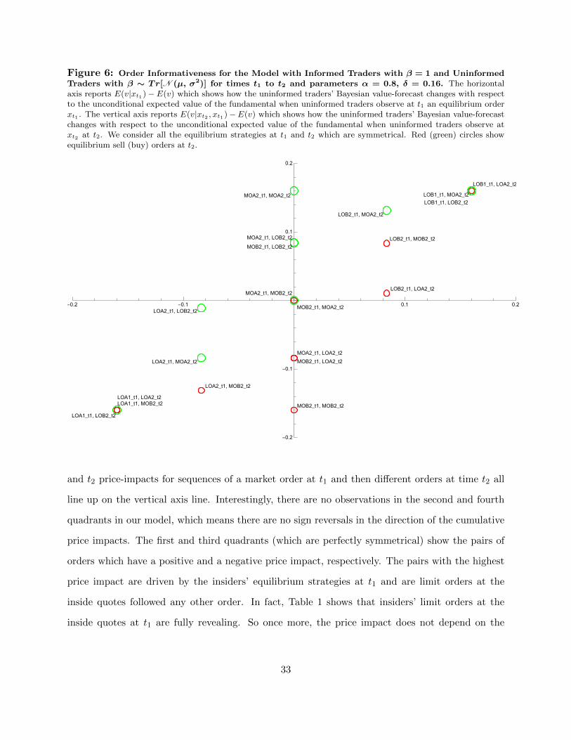
Figure 6: Order Informativeness for the Model with Informed Traders with β = 1 and UninformedTraders with β ∼ Tr[N (µ, σ2)] for times t1 to t2 and parameters α = 0.8, δ = 0.16. The horizontalaxis reports E(v|xt1)−E(v) which shows how the uninformed traders’ Bayesian value-forecast changes with respectto the unconditional expected value of the fundamental when uninformed traders observe at t1 an equilibrium orderxt1 . The vertical axis reports E(v|xt2 , xt1)−E(v) which shows how the uninformed traders’ Bayesian value-forecastchanges with respect to the unconditional expected value of the fundamental when uninformed traders observe atxt2 at t2. We consider all the equilibrium strategies at t1 and t2 which are symmetrical. Red (green) circles showequilibrium sell (buy) orders at t2.
and t2 price-impacts for sequences of a market order at t1 and then different orders at time t2 all
line up on the vertical axis line. Interestingly, there are no observations in the second and fourth
quadrants in our model, which means there are no sign reversals in the direction of the cumulative
price impacts. The first and third quadrants (which are perfectly symmetrical) show the pairs of
orders which have a positive and a negative price impact, respectively. The pairs with the highest
price impact are driven by the insiders’ equilibrium strategies at t1 and are limit orders at the
inside quotes followed any other order. In fact, Table 1 shows that insiders’ limit orders at the
inside quotes at t1 are fully revealing. So once more, the price impact does not depend on the
33
aggressiveness of the orders but on the informed investors’ orders choice. Overall, Figure 6 also
confirms that the price impact is non-Markovian: for example the price impact of MOB2 at t2 may
be either positive or negative depending on whether it is preceded by LOB2 or LOA2 at t1.
2.1.5 Summary
The analysis of our first model specification has identified a number of empirically testable predic-
tions. First, liquidity and the relative information content of different orders differ in high-volatility
markets (in which value shocks are large relative to the tick size) vs. in low-volatility markets (in
which value shocks are small relative to the tick size). Second, the price impact of order flow varies
conditional on different trading histories and on the standing book when new orders are submitted.
2.2 Informed and uninformed traders both have private-value motives
Our second model specification generalizes our earlier analysis so that now informed investors
also have random private-valuation factors β with the same truncated Normal distribution β ∼
Tr[N (µ, σ2)] as the uninformed investors. Hence, informed traders not only speculate on their
information, but they also have a private-value motive to trade. As a result, informed investors
with the same signal may end up buying and selling from each other. This combination of trading
motives has not been investigated in earlier models of dynamic limit order markets. We use our
second model specification to show the robustness of the results in Section 2.1 and to extend them.
2.2.1 Trading strategies
Tables 3 and 4 report order submission probabilities and other statistics for our second model
specification for time t1 by itself and for averages over times t2 through t4. Since all investors
have private-value motives to trade, all investors use all of the possible limit orders at time t1.
In particular, now informed investors also use market orders at t1. Over times t2 through t4, all
investors again use all types of limit orders and also market orders. In particular, directionally
informed investors trade sometimes opposite their asset-value information because their private-
value motive adds non-informational randomness to their orders. Informed investor with neutral
34
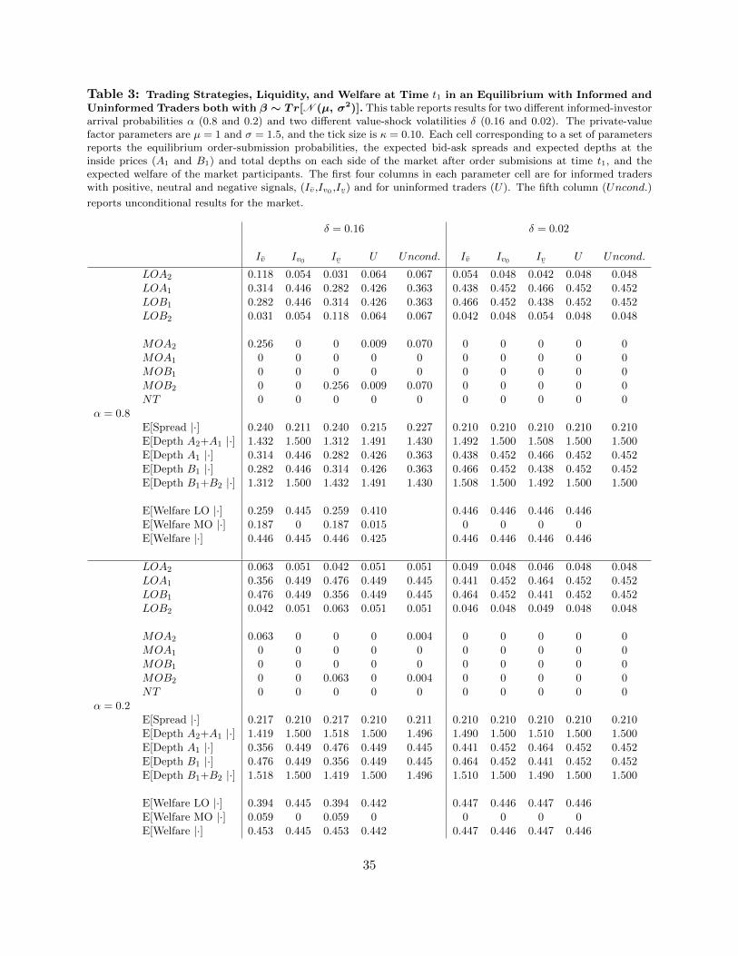
Table 3: Trading Strategies, Liquidity, and Welfare at Time t1 in an Equilibrium with Informed andUninformed Traders both with β ∼ Tr[N (µ, σ2)]. This table reports results for two different informed-investorarrival probabilities α (0.8 and 0.2) and two different value-shock volatilities δ (0.16 and 0.02). The private-valuefactor parameters are µ = 1 and σ = 1.5, and the tick size is κ = 0.10. Each cell corresponding to a set of parametersreports the equilibrium order-submission probabilities, the expected bid-ask spreads and expected depths at theinside prices (A1 and B1) and total depths on each side of the market after order submisions at time t1, and theexpected welfare of the market participants. The first four columns in each parameter cell are for informed traderswith positive, neutral and negative signals, (Iv,Iv0 ,Iv
¯) and for uninformed traders (U). The fifth column (Uncond.)
reports unconditional results for the market.
δ = 0.16 δ = 0.02
Iv Iv0 Iv¯
U Uncond. Iv Iv0 Iv¯
U Uncond.
LOA2 0.118 0.054 0.031 0.064 0.067 0.054 0.048 0.042 0.048 0.048LOA1 0.314 0.446 0.282 0.426 0.363 0.438 0.452 0.466 0.452 0.452LOB1 0.282 0.446 0.314 0.426 0.363 0.466 0.452 0.438 0.452 0.452LOB2 0.031 0.054 0.118 0.064 0.067 0.042 0.048 0.054 0.048 0.048
MOA2 0.256 0 0 0.009 0.070 0 0 0 0 0MOA1 0 0 0 0 0 0 0 0 0 0MOB1 0 0 0 0 0 0 0 0 0 0MOB2 0 0 0.256 0.009 0.070 0 0 0 0 0NT 0 0 0 0 0 0 0 0 0 0
α = 0.8E[Spread |·] 0.240 0.211 0.240 0.215 0.227 0.210 0.210 0.210 0.210 0.210E[Depth A2+A1 |·] 1.432 1.500 1.312 1.491 1.430 1.492 1.500 1.508 1.500 1.500E[Depth A1 |·] 0.314 0.446 0.282 0.426 0.363 0.438 0.452 0.466 0.452 0.452E[Depth B1 |·] 0.282 0.446 0.314 0.426 0.363 0.466 0.452 0.438 0.452 0.452E[Depth B1+B2 |·] 1.312 1.500 1.432 1.491 1.430 1.508 1.500 1.492 1.500 1.500
E[Welfare LO |·] 0.259 0.445 0.259 0.410 0.446 0.446 0.446 0.446E[Welfare MO |·] 0.187 0 0.187 0.015 0 0 0 0E[Welfare |·] 0.446 0.445 0.446 0.425 0.446 0.446 0.446 0.446
LOA2 0.063 0.051 0.042 0.051 0.051 0.049 0.048 0.046 0.048 0.048LOA1 0.356 0.449 0.476 0.449 0.445 0.441 0.452 0.464 0.452 0.452LOB1 0.476 0.449 0.356 0.449 0.445 0.464 0.452 0.441 0.452 0.452LOB2 0.042 0.051 0.063 0.051 0.051 0.046 0.048 0.049 0.048 0.048
MOA2 0.063 0 0 0 0.004 0 0 0 0 0MOA1 0 0 0 0 0 0 0 0 0 0MOB1 0 0 0 0 0 0 0 0 0 0MOB2 0 0 0.063 0 0.004 0 0 0 0 0NT 0 0 0 0 0 0 0 0 0 0
α = 0.2E[Spread |·] 0.217 0.210 0.217 0.210 0.211 0.210 0.210 0.210 0.210 0.210E[Depth A2+A1 |·] 1.419 1.500 1.518 1.500 1.496 1.490 1.500 1.510 1.500 1.500E[Depth A1 |·] 0.356 0.449 0.476 0.449 0.445 0.441 0.452 0.464 0.452 0.452E[Depth B1 |·] 0.476 0.449 0.356 0.449 0.445 0.464 0.452 0.441 0.452 0.452E[Depth B1+B2 |·] 1.518 1.500 1.419 1.500 1.496 1.510 1.500 1.490 1.500 1.500
E[Welfare LO |·] 0.394 0.445 0.394 0.442 0.447 0.446 0.447 0.446E[Welfare MO |·] 0.059 0 0.059 0 0 0 0 0E[Welfare |·] 0.453 0.445 0.453 0.442 0.447 0.446 0.447 0.446
35
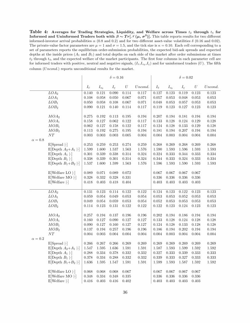
Table 4: Averages for Trading Strategies, Liquidity, and Welfare across Times t2 through t4 forInformed and Uninformed Traders both with β ∼ Tr[N (µ, σ2)]. This table reports results for two differentinformed-investor arrival probabilities α (0.8 and 0.2) and for two different asset-value volatilities δ (0.16 and 0.02).The private-value factor parameters are µ = 1 and σ = 1.5, and the tick size is κ = 0.10. Each cell corresponding to aset of parameters reports the equilibrium order-submission probabilities, the expected bid-ask spreads and expecteddepths at the inside prices (A1 and B1) and total depths on each side of the market after order submissions at timest2 through t4, and the expected welfare of the market participants. The first four columns in each parameter cell arefor informed traders with positive, neutral and negative signals, (Iv,Iv0 ,Iv
¯) and for uninformed traders (U). The fifth
column (Uncond.) reports unconditional results for the market.
δ = 0.16 δ = 0.02
Iv Iv0 Iv¯
U Uncond. Iv Iv0 Iv¯
U Uncond.
LOA2 0.140 0.121 0.090 0.114 0.117 0.127 0.123 0.119 0.123 0.123LOA1 0.108 0.058 0.050 0.067 0.071 0.057 0.053 0.048 0.053 0.053LOB1 0.050 0.058 0.108 0.067 0.071 0.048 0.053 0.057 0.053 0.053LOB2 0.090 0.121 0.140 0.114 0.117 0.119 0.123 0.127 0.123 0.123
MOA2 0.275 0.192 0.113 0.195 0.194 0.207 0.194 0.181 0.194 0.194MOA1 0.158 0.127 0.062 0.122 0.117 0.133 0.128 0.124 0.129 0.128MOB1 0.062 0.127 0.158 0.122 0.117 0.124 0.128 0.133 0.129 0.128MOB2 0.113 0.192 0.275 0.195 0.194 0.181 0.194 0.207 0.194 0.194NT 0.003 0.003 0.003 0.005 0.004 0.004 0.003 0.004 0.004 0.004
α = 0.8E[Spread |·] 0.253 0.259 0.253 0.274 0.259 0.268 0.269 0.268 0.269 0.268E[Depth A2+A1 |·] 1.599 1.600 1.537 1.563 1.576 1.590 1.593 1.596 1.593 1.593E[Depth A1 |·] 0.301 0.339 0.338 0.314 0.324 0.324 0.333 0.344 0.333 0.334E[Depth B1 |·] 0.338 0.339 0.301 0.314 0.324 0.344 0.333 0.324 0.333 0.334E[Depth B1+B2 |·] 1.537 1.600 1.599 1.563 1.576 1.596 1.593 1.590 1.593 1.593
E[Welfare LO |·] 0.089 0.071 0.089 0.072 0.067 0.067 0.067 0.067E[Welfare MO |·] 0.328 0.332 0.328 0.331 0.336 0.336 0.336 0.336E[Welfare |·] 0.418 0.403 0.418 0.404 0.403 0.403 0.403 0.403
LOA2 0.131 0.123 0.114 0.122 0.122 0.124 0.123 0.122 0.123 0.123LOA1 0.059 0.054 0.049 0.053 0.054 0.053 0.053 0.052 0.053 0.053LOB1 0.049 0.054 0.059 0.053 0.054 0.052 0.053 0.053 0.053 0.053LOB2 0.114 0.123 0.131 0.122 0.122 0.122 0.123 0.124 0.123 0.123
MOA2 0.257 0.194 0.137 0.196 0.196 0.202 0.194 0.186 0.194 0.194MOA1 0.160 0.127 0.090 0.127 0.127 0.133 0.128 0.124 0.128 0.128MOB1 0.090 0.127 0.160 0.127 0.127 0.124 0.128 0.133 0.128 0.128MOB2 0.137 0.194 0.257 0.196 0.196 0.186 0.194 0.202 0.194 0.194NT 0.004 0.003 0.004 0.004 0.004 0.004 0.003 0.004 0.004 0.004
α = 0.2E[Spread |·] 0.266 0.267 0.266 0.269 0.269 0.269 0.269 0.269 0.269 0.269E[Depth A2+A1 |·] 1.547 1.595 1.636 1.591 1.591 1.587 1.593 1.599 1.592 1.592E[Depth A1 |·] 0.288 0.334 0.378 0.332 0.332 0.327 0.333 0.339 0.333 0.333E[Depth B1 |·] 0.378 0.334 0.288 0.332 0.332 0.339 0.333 0.327 0.333 0.333E[Depth B1+B2 |·] 1.636 1.595 1.547 1.591 1.591 1.599 1.593 1.587 1.592 1.592
E[Welfare LO |·] 0.068 0.068 0.068 0.067 0.067 0.067 0.067 0.067E[Welfare MO |·] 0.348 0.334 0.348 0.335 0.336 0.336 0.336 0.336E[Welfare |·] 0.416 0.403 0.416 0.402 0.403 0.403 0.403 0.403
36
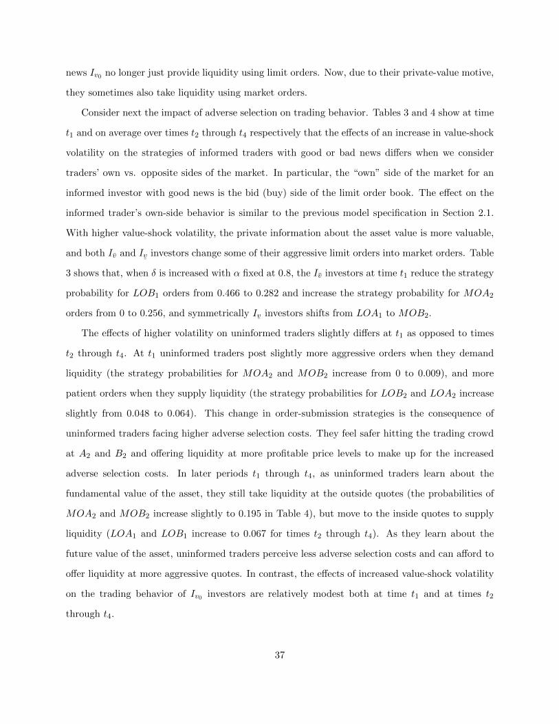
news Iv0 no longer just provide liquidity using limit orders. Now, due to their private-value motive,
they sometimes also take liquidity using market orders.
Consider next the impact of adverse selection on trading behavior. Tables 3 and 4 show at time
t1 and on average over times t2 through t4 respectively that the effects of an increase in value-shock
volatility on the strategies of informed traders with good or bad news differs when we consider
traders’ own vs. opposite sides of the market. In particular, the “own” side of the market for an
informed investor with good news is the bid (buy) side of the limit order book. The effect on the
informed trader’s own-side behavior is similar to the previous model specification in Section 2.1.
With higher value-shock volatility, the private information about the asset value is more valuable,
and both Iv and Iv¯
investors change some of their aggressive limit orders into market orders. Table
3 shows that, when δ is increased with α fixed at 0.8, the Iv investors at time t1 reduce the strategy
probability for LOB1 orders from 0.466 to 0.282 and increase the strategy probability for MOA2
orders from 0 to 0.256, and symmetrically Iv¯
investors shifts from LOA1 to MOB2.
The effects of higher volatility on uninformed traders slightly differs at t1 as opposed to times
t2 through t4. At t1 uninformed traders post slightly more aggressive orders when they demand
liquidity (the strategy probabilities for MOA2 and MOB2 increase from 0 to 0.009), and more
patient orders when they supply liquidity (the strategy probabilities for LOB2 and LOA2 increase
slightly from 0.048 to 0.064). This change in order-submission strategies is the consequence of
uninformed traders facing higher adverse selection costs. They feel safer hitting the trading crowd
at A2 and B2 and offering liquidity at more profitable price levels to make up for the increased
adverse selection costs. In later periods t1 through t4, as uninformed traders learn about the
fundamental value of the asset, they still take liquidity at the outside quotes (the probabilities of
MOA2 and MOB2 increase slightly to 0.195 in Table 4), but move to the inside quotes to supply
liquidity (LOA1 and LOB1 increase to 0.067 for times t2 through t4). As they learn about the
future value of the asset, uninformed traders perceive less adverse selection costs and can afford to
offer liquidity at more aggressive quotes. In contrast, the effects of increased value-shock volatility
on the trading behavior of Iv0 investors are relatively modest both at time t1 and at times t2
through t4.
37
The effects of an increase in the value-shock volatility is different on the opposite side than on
the own side. For example, when the volatility δ increases from 0.02 to 0.16, Iv investors at time t1
switch on the own side from LOB1 limit orders to aggressive MOA2 market orders but at the same
time they switch on the opposite side from aggressive limit orders to more patient limit orders. The
reason why Iv investors with low private-values become more patient when selling via limit orders
on the opposite side is that they know that the execution probability of limit sells at A2 is higher
because other Iv investors in future periods will hit limit sell orders at A2 more aggressively given
that v is much bigger (see the increased order submission probabilities for MOA2 in Table 4).
2.2.2 Market quality
The effect of value-shock volatility on market liquidity is mixed in our second model specification.
This is not surprising given the different effects of increased volatility on informed-investor trading
behavior on the own and opposite sides of the market. At time t1, holding the informed-investor
arrival probability α fixed, increased value-shock volatility leads to wider spreads and less total
depth. However, the average effects over times t2 through t4 switches with increased asset-value
volatility leading now to narrower spreads and smaller depth. This is due — in particular in the high
α markets — to uninformed traders perceiving greater adverse selction costs and therefore being
less willing to supply liquidity. Interestingly, the effects of an increase in the arrival probability of
informed investors (α) on the equilibrium strategies is qualitatively similar to that of an increase
in volatility (δ) in this second model specification.
Lastly, our model shows how an increase in volatility and in the proportion of insiders affect
the welfare of market participants. When volatility increases, directional informed investors are
generally better off as their signal is stronger and hence more profitable: At t1 their welfare is
unchanged with high proportion of insiders (0.446), whereas it increases in all the other scenarios,
with low proportion of insiders (0.453) and in later periods with both high and low α (0.418 and
0.416). At t1 uninformed traders are worse off because liquidity deteriorates with higher volatility.
At later periods the result is ambiguous: there are cases in which the uninformed investors are
better off and cases in which they are worse off.
38
2.2.3 Information content of orders
Figure 7 plots the Bayesian revisions for different orders at time t1 against the corresponding order-
execution probabilities for our second model specification. Once again, the magnitudes and signs
of the Bayesian updates depends on the mix of informed and uninformed investors who submit
these orders. Consider, for example, the market with both high value-shock volatility and a high
informed-investor arrival probability (large circles). The most informative orders are the market
orders MOA2 and MOB2 as they are chosen much more often by informed investors than by
uninformed investors (See Table 3). However, the next most aggressive orders are the inside limit
orders LOB1 and LOA1, and they are less informative than the less aggressive LOB2 and LOA2
limit orders. Even though the aggressive limit orders LOB1 and LOA1 are posted with a relatively
high probability (0.282 and 0.314) by informed investors Iv and Iv, they are also submitted with
even high probabilities by uninformed investors (0.426), and Iv0 informed investors with neutral
(0.446). As a result, they are less informative.15 Thus, this is another example in which order
informativeness is not increasing in order aggressiveness.
Perhaps more surprisingly, the order-sign conjecture need not hold in our second model spe-
cification:
Result 5 The Bayesian value revision can be opposite the direction of an order.
This is to say that the direction of orders is sometimes different from the sign of their information
content. For example, a limit sell LOA1 signals good news (rather than bad news as one might
expect) because limit sells at A1 are used by informed investor to trade on the opposite side of
their information (i.e., due to their private-value β factors) more frequently than these orders are
used to trade on the same side of their information. In particular, Iv investors usually sell using
market orders MOB2 rather than using limit sells. This goes back to our previous discussion of
how informed investors trade differently on the own side of their information (when their private
value β reinforces the trading direction from their information) and on the opposite side of their
information (when their β reverses the trading incentive from their information).
15The informativeness of limit orders LOA1 and LOB1 in Table B2 in Appendix B are 0.004 and−0.004 respectively,whereas the informativeness of limit orders LOA2 and LOB2 are 0.056 and −0.056 respectively.
39
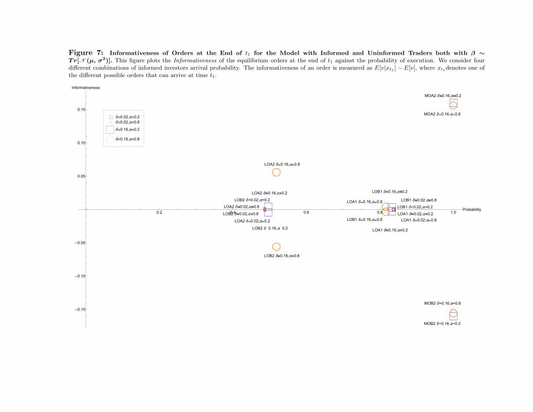
Figure 7: Informativeness of Orders at the End of t1 for the Model with Informed and Uninformed Traders both with β ∼Tr[N (µ, σ2)]. This figure plots the Informativeness of the equilibrium orders at the end of t1 against the probability of execution. We consider fourdifferent combinations of informed investors arrival probability. The informativeness of an order is measured as E[v|xt1 ]− E[v], where xt1denotes one ofthe different possible orders that can arrive at time t1.
MOA2 δ 0.16,α 0.2
MOB2 δ 0.16,α 0.2
LOA2 δ 0.16,α 0.2
LOA1 δ 0.16,α 0.2
LOB1 δ 0.16,α 0.2
LOB2 δ 0.16,α 0.2
LOA2 δ 0.02,α 0.2
LOA1 δ 0.02,α 0.2
LOB1 δ 0.02,α 0.2
LOB2 δ 0.02,α 0.2
MOA2 δ 0.16,α 0.8
LOA2 δ 0.16,α 0.8
LOA1 δ 0.16,α 0.8
LOB1 δ 0.16,α 0.8
LOB2 δ 0.16,α 0.8
MOB2 δ 0.16,α 0.8
LOA1 δ 0.02,α 0.8
LOB1 δ 0.02,α 0.8
LOA2 δ 0.02,α 0.8
LOB2 δ 0.02,α 0.80.2 0.4 0.6 0.8 1.0Probability
-0.15
-0.10
-0.05
0.05
0.10
0.15
Informativeness
δ=0.02,α=0.2
δ=0.02,α=0.8
δ=0.16,α=0.2
δ=0.16,α=0.8
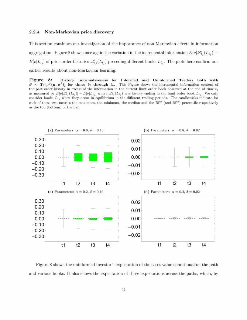
2.2.4 Non-Markovian price discovery
This section continues our investigation of the importance of non-Markovian effects in information
aggregation. Figure 8 shows once again the variation in the incremental information E[v|Ltj (Ltj )]−
E[v|Ltj ] of prior order histories Ltj (Ltj ) preceding different books Ltj . The plots here confirm our
earlier results about non-Markovian learning.
Figure 8: History Informativeness for Informed and Uninformed Traders both withβ ∼ Tr[N (µ, σ2)] for times t2 through t4. This Figure shows the incremental information content ofthe past order history in excess of the information in the current limit order book observed at the end of time tjas measured by E[v|Ltj (Ltj )] − E[v|Ltj ] where Ltj (Ltj ) is a history ending in the limit order book Ltj . We onlyconsider books Ltj when they occur in equilibrium in the different trading periods. The candlesticks indicate for
each of these two metrics the maximum, the minimum, the median and the 75th (and 25th) percentile respectivelyas the top (bottom) of the bar.
(a) Parameters: α = 0.8, δ = 0.16
t1 t2 t3 t4
-0.30
-0.20
-0.10
0.00
0.10
0.20
0.30
(b) Parameters: α = 0.8, δ = 0.02
t1 t2 t3 t4
-0.02
-0.01
0.00
0.01
0.02
(c) Parameters: α = 0.2, δ = 0.16
t1 t2 t3 t4
-0.30
-0.20
-0.10
0.00
0.10
0.20
0.30
(d) Parameters: α = 0.2, δ = 0.02
t1 t2 t3 t4
-0.02
-0.01
0.00
0.01
0.02
Figure 8 shows the uninformed investor’s expectation of the asset value conditional on the path
and various books. It also shows the expectation of these expectations across the paths, which, by
41
iterated expectation, is the expectation conditional on the book. Again, we see that the trading
history has substantial information content above and beyond the information in the book alone.
The figure also shows the standard deviation of the valuation forecast errors. Here again, the
information updating dynamics are non-Markovian.
2.3 Summary
The results for our second model specification — with a richer specification of the informed investors’
trading motives — confirm and extent the analysis from our first model specification.
• When all market participants trade not only to speculate on their signal but also to satisfy
their private-value motive, all investors use both market and limit orders in equilibrium.
• Increased adverse selection affects informed-investor trading behavior differently when they
trade with their information versus (because of private-value shocks) against their informa-
tion. As a result, the effect of asset-value volatility and informed investor arrival probability
on market liquidity is mixed.
• The informativeness of orders can be opposite the order aggressiveness and now also the order
direction. The information content of order arrivals is again history-dependent.
3 Robustness
Our analysis makes a number of simplifying assumptions for tractability, but we conjecture that our
qualitative results are robust to relaxing these assumptions. We consider two of these assumptions
here. First, our model of the trading day only has five periods. Relatedly, our analysis abstracts
from limit orders being carried over from one day to the next. However, our results about the impact
of adverse selection on investor trading strategies and about order informativeness are driven in
large part by the relative size of information shocks and the tick size rather than by the number
of rounds of trading. In addition, increasing the trading horizon leads to longer histories that are
potentially even more informative. Second, arriving investors are only allowed to submit single
orders that cannot be cancelled or modified subsequently. However, it seems likely that order-flow
42

histories will still be informative if orders at different points in time are correlated due to correlated
actions of returning investors.
4 Conclusions
This paper has studied information aggregation and liquidity provision in dynamic limit order
markets. We show a number of notable theoretical properties in our model. First, informed investors
switch between endogenously demanding liquidity via market orders and supplying liquidity via
limit orders. Second, the information content/price impact of orders can be non-monotone in the
direction of the order and in the aggressiveness of their orders. Third, the information aggregation
process is non-Markovian. In particular, the prior order history has information content beyond
that in the current limit order book.
Our model suggests several directions for future research. Most importantly, our analysis
provides a framework for empirical research about the changing price impacts of order flow condi-
tional on order-flow history and time of day. There are also promising directions for future theory.
First, the model can be enriched by allowing investors to trade dynamically over time (rather
than just submitting an order one time) and to face quantity decisions and to use multiple orders.
Second, the model could be extended to allow for trading in multiple co-existing limit order mar-
kets. This would be a realistic representation of current equity trading in the US. Third, the model
could be used to study high frequency trading in limit order markets and the effect of different
investors being able to process and trade on different types of information at different latencies.
5 Appendix A: Algorithm for computing equilibrium
The computational problem to solve for a Perfect Bayesian Nash equilibrium in our model (as
defined in Section 1.1) is complex. Given investors’ equilibrium beliefs, the optimal order-submission
problems in (6) and (7) require computing limit-order execution probabilities and stock-value ex-
pectations that are conditional on both the past order history and on future state-contingent limit-
order execution at each time tj at each node of the trading game. For an informed trader (who
43
knows the asset value v), there is no uncertainty about the payoff of a market order. In contrast, the
payoff of a market order for an uninformed trader entails uncertainty about the future asset value
and, therefore, computing the optimal order requires computing the expected stock value E[v|Ltj−1 ]
conditional on the prior trading history up to time tj . For limit orders, the expected payoff depends
on the future limit-order execution probabilities, Pr(θxtj |v,Ltj−1) and Pr(θxtj |Ltj−1), for informed
and uninformed investors, which depend, in turn, on the optimal order-submission probabilities of
future informed and uninformed investors. In addition, the uninformed investors’ learning problem
for limit orders requires uninformed investors to extract information about the expected future
stock value E[v|Ltj−1 , θxtj ] from both the past trading history and also from state-contingent future
order execution given that the future states in which limit orders are executed are correlated with
the stock value. Thus, optimal actions at each time tj depend on past information and future
order-flow contingencies where future orders also depend on the then-prior histories at future dates
(which include the action at time tj) as traders dynamically update their equilibrium beliefs as the
trading process unfolds. Thus, the learning problem for limit order beliefs is both backward- and
forward-looking. Lastly, rational expectations (RE) involves finding a fixed point so that the equi-
librium beliefs underlying the optimal order-submission strategies are consistent with the execution
probabilities and value expectations that the endogenous optimal strategies produce in equilibrium.
Our numerical algorithm uses backward induction to solve for optimal order strategies given a
set of asset-value beliefs for all dates and nodes in the trading game and uses an iterative recursion
to solve for RE equilibrium asset-value and order-execution beliefs. The backward induction makes
order-execution probabilities consistent with optimal future behavior by later-arriving investors. It
also takes future state-contingent execution into account in the uninformed investors’ beliefs. Given
a set of history-contingent asset-value probability beliefs, we start at time t5 — when traders only
use market orders which allows us to compute the execution probabilities of limit orders at t4 —
and recursively solve the model for optimal order strategies back to time t1. We then embed the
optimal order strategy calculation in an iterative recursion to solve for a fixed point for the RE
asset-value beliefs. For a generic round r in this recursion, the outgoing asset-value probabilities
πv,r−1tj
from round r−1 are used iteratively as incoming asset-value beliefs in round r. In particular,
44
these beliefs are used in the learning problem of the uninformed investor to extract information
about the ending asset value v from the prior trading histories. They also affect the behavior
of informed investors whose order-execution probability beliefs depend in part on the behavior
of uninformed traders. Thus, the recursion for a generic round r involves solving by backward
induction for optimal strategies for buyers
maxx∈Xtj
wI, r(x | v,Ltj−1) = [βtj v0 + ∆− p(x)]Prr(θxtj | v,Ltj−1) (13)
and
maxx∈Xtj
wU, r(x |Ltj−1) = [βtj v0 + Er[∆ |Ltj−1 , θxtj ]− p(x)]Prr(θxtj |Ltj−1) (14)
where
Er[∆|Ltj−1 , θxtj ] = (πv, rtj
v + πv0, rtj
v0 + πv, rtjv)− v0 (15)
πv, rtj=
Prr(θxtj |v,Ltj )
Prr(θxtj |Ltj )πv, r−1tj
(16)
and where the calculations for sellers are symmetric. Note that at each time tj the backward
induction has already determined the future contingencies θxtj for limit order executions at times t >
tj . Thus, the order-execution probabilities Prr(θxtj | v,Ltj−1) and Prr(θxtj |Ltj−1), and the history-
and execution-contingent probabilities πv, rtjand associated asset-value expectations Er[∆|Ltj−1 , θ
xtj ]
are “mongrel” moments in that they are computed using the outgoing history-contingent asset value
beliefs πv, r−1tj
from round r−1 and then updated given the order-execution contingencies computed
by backward induction in round r using the round r− 1 asset-value beliefs. At the end of round r,
we then compute updated outgoing asset-value beliefs πv,rtj for round r, which are used as incoming
beliefs for the next round r + 1. The recursion is iterated to find a RE fixed point πvtj in the
uninformed investor beliefs.
The fixed-point recursion is started in round r = 1 by setting the initial asset-value beliefs πv,0tj
of uninformed traders at each time tj in the backward induction to be the unconditional priors
45
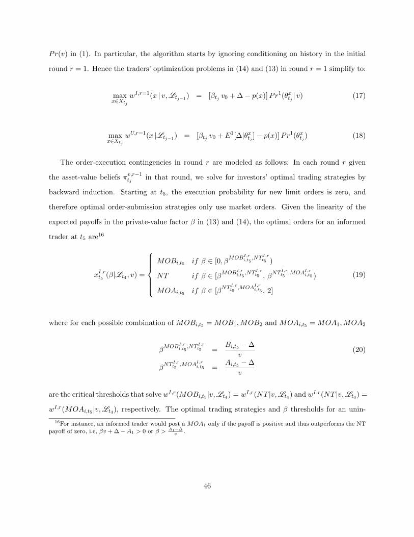
Pr(v) in (1). In particular, the algorithm starts by ignoring conditioning on history in the initial
round r = 1. Hence the traders’ optimization problems in (14) and (13) in round r = 1 simplify to:
maxx∈Xtj
wI,r=1(x | v,Ltj−1) = [βtj v0 + ∆− p(x)]Pr1(θxtj | v) (17)
maxx∈Xtj
wU,r=1(x |Ltj−1) = [βtj v0 + E1[∆|θxtj ]− p(x)]Pr1(θxtj ) (18)
The order-execution contingencies in round r are modeled as follows: In each round r given
the asset-value beliefs πv,r−1tj
in that round, we solve for investors’ optimal trading strategies by
backward induction. Starting at t5, the execution probability for new limit orders is zero, and
therefore optimal order-submission strategies only use market orders. Given the linearity of the
expected payoffs in the private-value factor β in (13) and (14), the optimal orders for an informed
trader at t5 are16
xI,rt5 (β|Lt4 , v) =
MOBi,t5 if β ∈ [0, β
MOBI,ri,t5
,NT I,rt5 )
NT if β ∈ [βMOBI,r
i,t5,NT I,r
t5 , βNT I,r
t5,MOAI,r
i,t5 )
MOAi,t5 if β ∈ [βNT I,r
t5,MOAI,r
i,t5 , 2]
(19)
where for each possible combination of MOBi,t5 = MOB1,MOB2 and MOAi,t5 = MOA1,MOA2
βMOBI,r
i,t5,NT I,r
t5 =Bi,t5 −∆
v(20)
βNT I,r
t5,MOAI,r
i,t5 =Ai,t5 −∆
v
are the critical thresholds that solve wI,r(MOBi,t5 |v,Lt4) = wI,r(NT |v,Lt4) and wI,r(NT |v,Lt4) =
wI,r(MOAi,t5 |v,Lt4), respectively. The optimal trading strategies and β thresholds for an unin-
16For instance, an informed trader would post a MOA1 only if the payoff is positive and thus outperforms the NTpayoff of zero, i.e, βv + ∆−A1 > 0 or β > A1−∆
v.
46
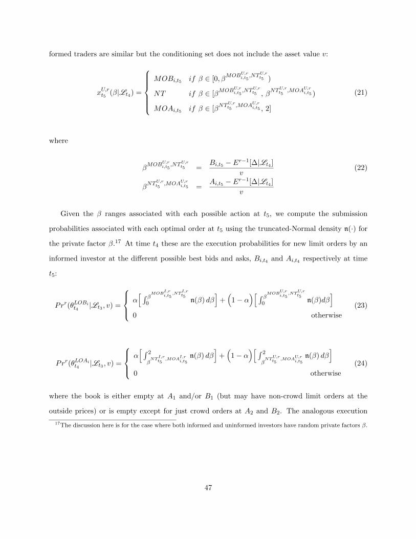
formed traders are similar but the conditioning set does not include the asset value v:
xU,rt5 (β|Lt4) =
MOBi,t5 if β ∈ [0, β
MOBU,ri,t5
,NTU,rt5 )
NT if β ∈ [βMOBU,r
i,t5,NTU,r
t5 , βNTU,r
t5,MOAU,r
i,t5 )
MOAi,t5 if β ∈ [βNTU,r
t5,MOAU,r
i,t5 , 2]
(21)
where
βMOBU,r
i,t5,NTU,r
t5 =Bi,t5 − Er−1[∆|Lt4 ]
v(22)
βNTU,r
t5,MOAU,r
i,t5 =Ai,t5 − Er−1[∆|Lt4 ]
v
Given the β ranges associated with each possible action at t5, we compute the submission
probabilities associated with each optimal order at t5 using the truncated-Normal density n(·) for
the private factor β.17 At time t4 these are the execution probabilities for new limit orders by an
informed investor at the different possible best bids and asks, Bi,t4 and Ai,t4 respectively at time
t5:
Prr(θLOBit4
|Lt3 , v) =
α[ ∫ βMOB
I,ri,t5
,NTI,rt5
0 n(β) dβ]
+(
1− α)[ ∫ βMOB
U,ri,t5
,NTU,rt5
0 n(β)dβ]
0 otherwise
(23)
Prr(θLOAit4
|Lt3 , v) =
α[ ∫ 2
βNT
I,rt5
,MOAI,ri,t5
n(β) dβ]
+(
1− α)[ ∫ 2
βNT
U,rt5
,MOAU,ri,t5
n(β) dβ]
0 otherwise
(24)
where the book is either empty at A1 and/or B1 (but may have non-crowd limit orders at the
outside prices) or is empty except for just crowd orders at A2 and B2. The analogous execution
17The discussion here is for the case where both informed and uninformed investors have random private factors β.
47
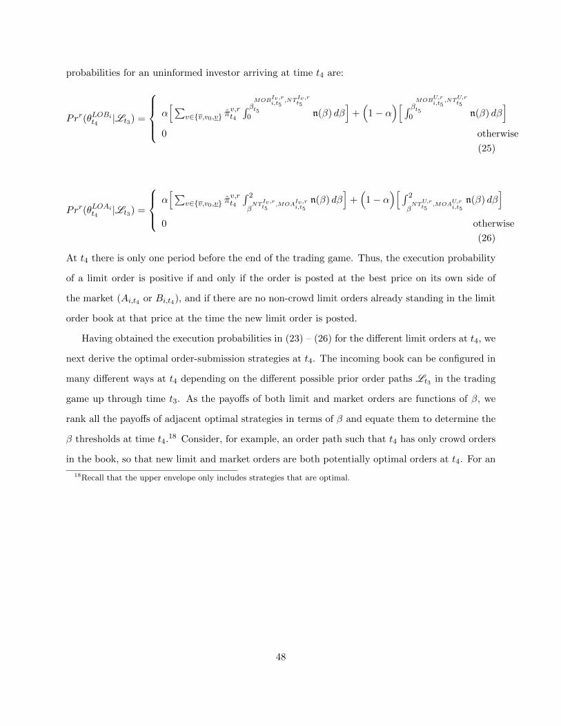
probabilities for an uninformed investor arriving at time t4 are:
Prr(θLOBit4
|Lt3) =
α[∑
v∈{v,v0,v} πv,rt4
∫ βMOBIv,ri,t5
,NTIv,rt5
t50 n(β) dβ
]+(
1− α)[ ∫ βMOB
U,ri,t5
,NTU,rt5
t50 n(β) dβ
]0 otherwise
(25)
Prr(θLOAit4
|Lt3) =
α[∑
v∈{v,v0,v} πv,rt4
∫ 2
βNT
Iv,rt5
,MOAIv,ri,t5
n(β) dβ]
+(
1− α)[ ∫ 2
βNT
U,rt5
,MOAU,ri,t5
n(β) dβ]
0 otherwise
(26)
At t4 there is only one period before the end of the trading game. Thus, the execution probability
of a limit order is positive if and only if the order is posted at the best price on its own side of
the market (Ai,t4 or Bi,t4), and if there are no non-crowd limit orders already standing in the limit
order book at that price at the time the new limit order is posted.
Having obtained the execution probabilities in (23) – (26) for the different limit orders at t4, we
next derive the optimal order-submission strategies at t4. The incoming book can be configured in
many different ways at t4 depending on the different possible prior order paths Lt3 in the trading
game up through time t3. As the payoffs of both limit and market orders are functions of β, we
rank all the payoffs of adjacent optimal strategies in terms of β and equate them to determine the
β thresholds at time t4.18 Consider, for example, an order path such that t4 has only crowd orders
in the book, so that new limit and market orders are both potentially optimal orders at t4. For an
18Recall that the upper envelope only includes strategies that are optimal.
48
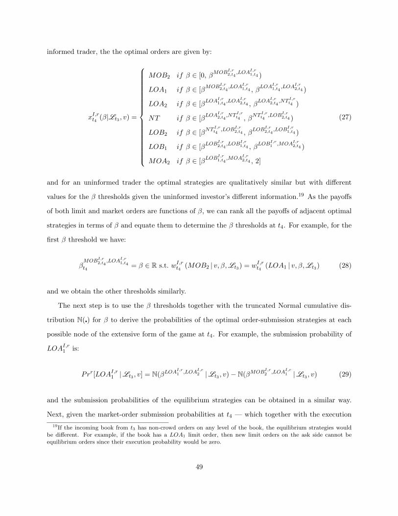
informed trader, the the optimal orders are given by:
xI,rt4 (β|Lt3 , v) =
MOB2 if β ∈ [0, βMOBI,r
2,t4,LOAI,r
1,t4 )
LOA1 if β ∈ [βMOBI,r
2,t4,LOAI,r
1,t4 , βLOAI,r
1,t4,LOAI,r
2,t4 )
LOA2 if β ∈ [βLOAI,r
1,t4,LOAI,r
2,t4 , βLOAI,r
2,t4,NT I,r
t4 )
NT if β ∈ [βLOAI,r
2,t4,NT I,r
t4 , βNT I,r
t4,LOBI,r
2,t4 )
LOB2 if β ∈ [βNT I,r
t4,LOBI,r
2,t4 , βLOBI,r
2,t4,LOBI,r
1,t4 )
LOB1 if β ∈ [βLOBI,r
2,t4,LOBI,r
1,t4 , βLOBI,r
1 ,MOAI,r2,t4 )
MOA2 if β ∈ [βLOBI,r
1,t4,MOAI,r
2,t4 , 2]
(27)
and for an uninformed trader the optimal strategies are qualitatively similar but with different
values for the β thresholds given the uninformed investor’s different information.19 As the payoffs
of both limit and market orders are functions of β, we can rank all the payoffs of adjacent optimal
strategies in terms of β and equate them to determine the β thresholds at t4. For example, for the
first β threshold we have:
βMOBI,r
2,t4,LOAI,r
1,t4t4
= β ∈ R s.t. wI,rt4 (MOB2 | v, β,Lt3) = wI,rt4 (LOA1 | v, β,Lt3) (28)
and we obtain the other thresholds similarly.
The next step is to use the β thresholds together with the truncated Normal cumulative dis-
tribution N(�) for β to derive the probabilities of the optimal order-submission strategies at each
possible node of the extensive form of the game at t4. For example, the submission probability of
LOAI,r1 is:
Prr[LOAI,r1 |Lt3 , v] = N(βLOAI,r1 ,LOAI,r
2 |Lt3 , v)− N(βMOBI,r2 ,LOAI,r
1 |Lt3 , v) (29)
and the submission probabilities of the equilibrium strategies can be obtained in a similar way.
Next, given the market-order submission probabilities at t4 — which together with the execution
19If the incoming book from t3 has non-crowd orders on any level of the book, the equilibrium strategies wouldbe different. For example, if the book has a LOA1 limit order, then new limit orders on the ask side cannot beequilibrium orders since their execution probability would be zero.
49
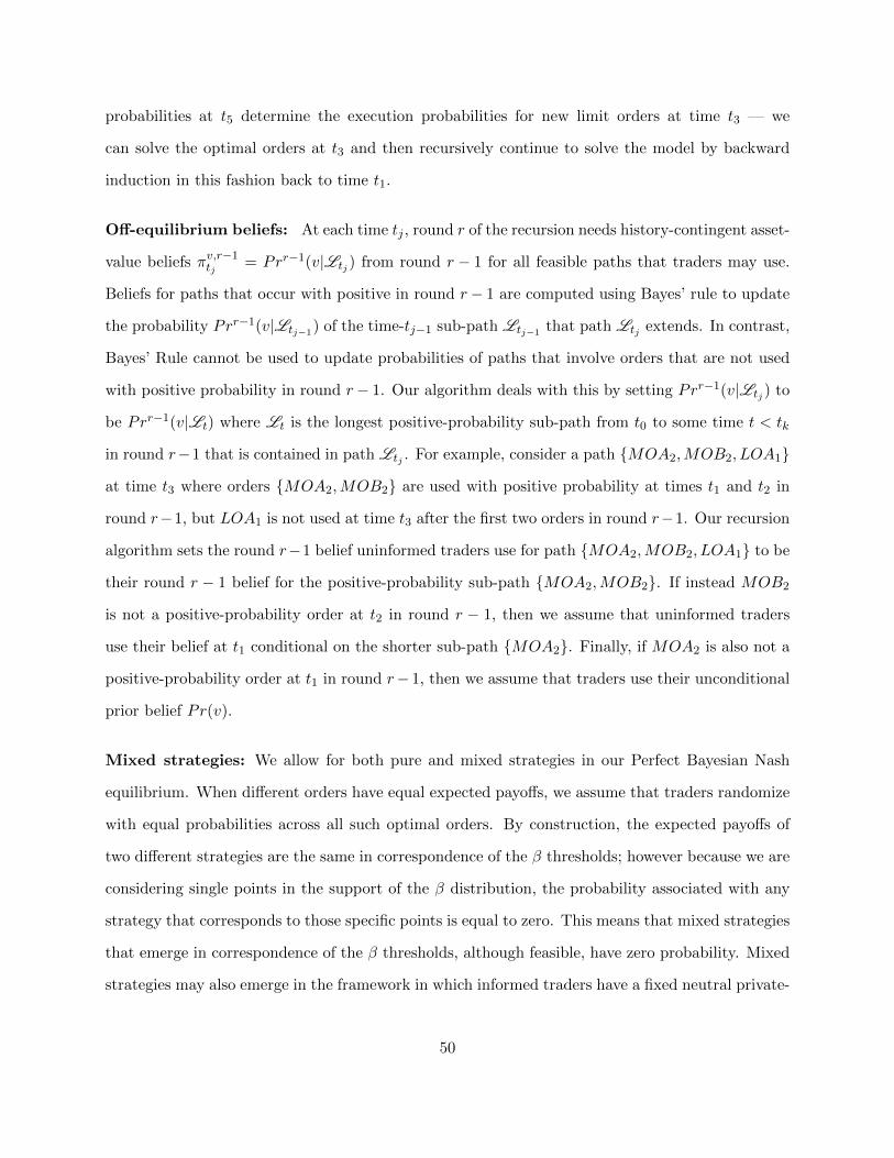
probabilities at t5 determine the execution probabilities for new limit orders at time t3 — we
can solve the optimal orders at t3 and then recursively continue to solve the model by backward
induction in this fashion back to time t1.
Off-equilibrium beliefs: At each time tj , round r of the recursion needs history-contingent asset-
value beliefs πv,r−1tj
= Prr−1(v|Ltj ) from round r − 1 for all feasible paths that traders may use.
Beliefs for paths that occur with positive in round r− 1 are computed using Bayes’ rule to update
the probability Prr−1(v|Ltj−1) of the time-tj−1 sub-path Ltj−1 that path Ltj extends. In contrast,
Bayes’ Rule cannot be used to update probabilities of paths that involve orders that are not used
with positive probability in round r− 1. Our algorithm deals with this by setting Prr−1(v|Ltj ) to
be Prr−1(v|Lt) where Lt is the longest positive-probability sub-path from t0 to some time t < tk
in round r−1 that is contained in path Ltj . For example, consider a path {MOA2,MOB2, LOA1}
at time t3 where orders {MOA2,MOB2} are used with positive probability at times t1 and t2 in
round r−1, but LOA1 is not used at time t3 after the first two orders in round r−1. Our recursion
algorithm sets the round r−1 belief uninformed traders use for path {MOA2,MOB2, LOA1} to be
their round r − 1 belief for the positive-probability sub-path {MOA2,MOB2}. If instead MOB2
is not a positive-probability order at t2 in round r − 1, then we assume that uninformed traders
use their belief at t1 conditional on the shorter sub-path {MOA2}. Finally, if MOA2 is also not a
positive-probability order at t1 in round r− 1, then we assume that traders use their unconditional
prior belief Pr(v).
Mixed strategies: We allow for both pure and mixed strategies in our Perfect Bayesian Nash
equilibrium. When different orders have equal expected payoffs, we assume that traders randomize
with equal probabilities across all such optimal orders. By construction, the expected payoffs of
two different strategies are the same in correspondence of the β thresholds; however because we are
considering single points in the support of the β distribution, the probability associated with any
strategy that corresponds to those specific points is equal to zero. This means that mixed strategies
that emerge in correspondence of the β thresholds, although feasible, have zero probability. Mixed
strategies may also emerge in the framework in which informed traders have a fixed neutral private-
50

value factor β = 1 (section 2.1). More specifically it may happen that the payoffs of two perfectly
symmetrical strategies of Iv0 are the same, and in this case Iv0 randomizes between these two
strategies.
In the setting of our model where informed traders have fixed neutral private-value factors
β = 1, it may happen that both informed and uninformed traders switch their strategies back and
forth from one round to the next. When this happens, to reach an equilibrium we assume that
the informed traders play mixed strategies and at each subsequent round strategically reduce the
probability with which they choose the most profitable strategy until the equilibrium is reached.
As an example at t1 informed traders with positive news, Iv, play LOB2 in round r = 1. However,
in round r = 2 in the subsequent periods uninformed traders do not send market orders to sell at
B2 and in round r = 3, informed traders react by changing their strategy to LOB1. However, in the
subsequent periods uninformed traders do not send market orders to sell, this time at B1. To find
an equilibrium, we assume that at each round informed traders play mixed strategies and assign
a greater weight to the most profitable strategy. In this case we assume they start playing LOB2
with probability 0.99 and LOB1 with probability 0.01. If these mixed strategies do not lead to
an equilibrium outcome, in the subsequent round we assume that the informed traders play LOB2
with probability 0.98 and LOB1 with probability 0.02. We proceed by lowering the probability
with which informed traders choose the most profitable strategy until we reach an equilibrium set
of strategies.
Convergence: RE beliefs for a Perfect Bayesian Nash equilibrium are obtained by solving the
model recursively for multiple rounds. In particular, the asset-value probabilities πv,1tj from round
r = 1 from above are used as the priors to solve the model in round r = 2 (i.e., the round 1
probabilities are used in place of the unconditional priors used in round 1).20 The asset-value
probabilities πv,2tj from round r = 2 are then used as the priors in round r = 3 and so on. The
recursive iteration is continued until the updating process converges to a fixed point, which are the
RE beliefs. In particular, the recursive process has converged to the RE beliefs when uninformed
traders no longer revise their asset-value beliefs. Operationally, we consider convergence to the RE
20In the second round of solutions we again solve the full 5-period model.
51
beliefs to have occurred when the probabilities πv, rtj, πv0, r
tjand π
v, rtj
in round r are “close enough”
to the corresponding probabilities from round r − 1:
πv, ∗tj when∣∣∣πv, rtj
− πv, r−1tj
∣∣∣ < 10−7
πv0, ∗tj
when∣∣∣πv0, rtj− πv0, r−1
tj
∣∣∣ < 10−7
πv, ∗tj
when∣∣∣πv, rtj
− πv, r−1tj
∣∣∣ < 10−7
(30)
A fixed-point solution to this recursive algorithm is an equilibrium in our model.
6 Appendix B: Additional numerical results
The tables is this section provide additional information on the execution probabilities of limit
orders for informed investor with positive, neutral and negative signals, (Iv,Iv0 ,Iv¯) and for unin-
formed traders. The tables also report the asset value expectations of the uninformed investor at
time t2 after observing all the possible buy orders submissions at time t1. The expectations for sell
orders are symmetric with respect to 1. Table B1 reports results for our first model specification
in which only uninformed traders have a random private value factor. Table B2 reports results for
our second model in which both the informed and uniformed traders have private-value motives.
52
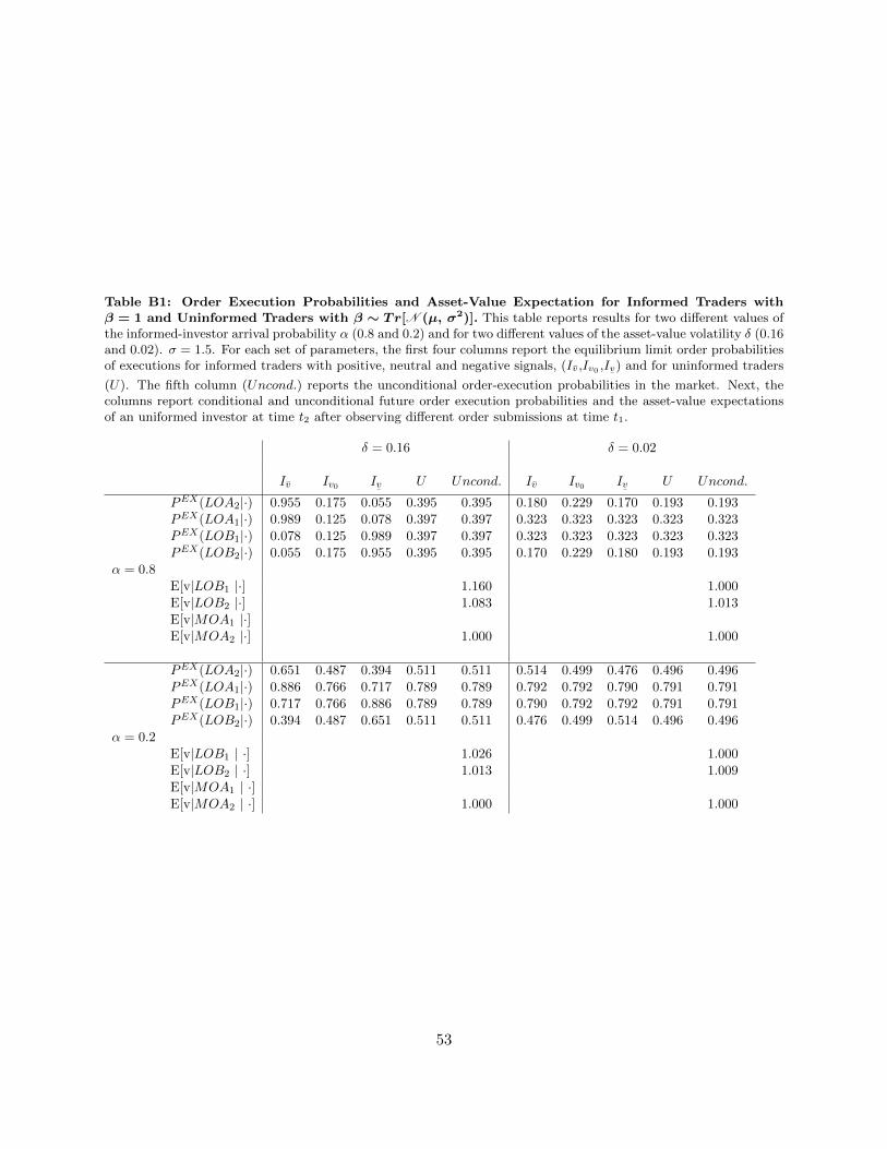
Table B1: Order Execution Probabilities and Asset-Value Expectation for Informed Traders withβ = 1 and Uninformed Traders with β ∼ Tr[N (µ, σ2)]. This table reports results for two different values ofthe informed-investor arrival probability α (0.8 and 0.2) and for two different values of the asset-value volatility δ (0.16and 0.02). σ = 1.5. For each set of parameters, the first four columns report the equilibrium limit order probabilitiesof executions for informed traders with positive, neutral and negative signals, (Iv,Iv0 ,Iv
¯) and for uninformed traders
(U). The fifth column (Uncond.) reports the unconditional order-execution probabilities in the market. Next, thecolumns report conditional and unconditional future order execution probabilities and the asset-value expectationsof an uniformed investor at time t2 after observing different order submissions at time t1.
δ = 0.16 δ = 0.02
Iv Iv0 Iv¯
U Uncond. Iv Iv0 Iv¯
U Uncond.
PEX(LOA2|·) 0.955 0.175 0.055 0.395 0.395 0.180 0.229 0.170 0.193 0.193PEX(LOA1|·) 0.989 0.125 0.078 0.397 0.397 0.323 0.323 0.323 0.323 0.323PEX(LOB1|·) 0.078 0.125 0.989 0.397 0.397 0.323 0.323 0.323 0.323 0.323PEX(LOB2|·) 0.055 0.175 0.955 0.395 0.395 0.170 0.229 0.180 0.193 0.193
α = 0.8E[v|LOB1 |·] 1.160 1.000E[v|LOB2 |·] 1.083 1.013E[v|MOA1 |·]E[v|MOA2 |·] 1.000 1.000
PEX(LOA2|·) 0.651 0.487 0.394 0.511 0.511 0.514 0.499 0.476 0.496 0.496PEX(LOA1|·) 0.886 0.766 0.717 0.789 0.789 0.792 0.792 0.790 0.791 0.791PEX(LOB1|·) 0.717 0.766 0.886 0.789 0.789 0.790 0.792 0.792 0.791 0.791PEX(LOB2|·) 0.394 0.487 0.651 0.511 0.511 0.476 0.499 0.514 0.496 0.496
α = 0.2E[v|LOB1 | ·] 1.026 1.000E[v|LOB2 | ·] 1.013 1.009E[v|MOA1 | ·]E[v|MOA2 | ·] 1.000 1.000
53
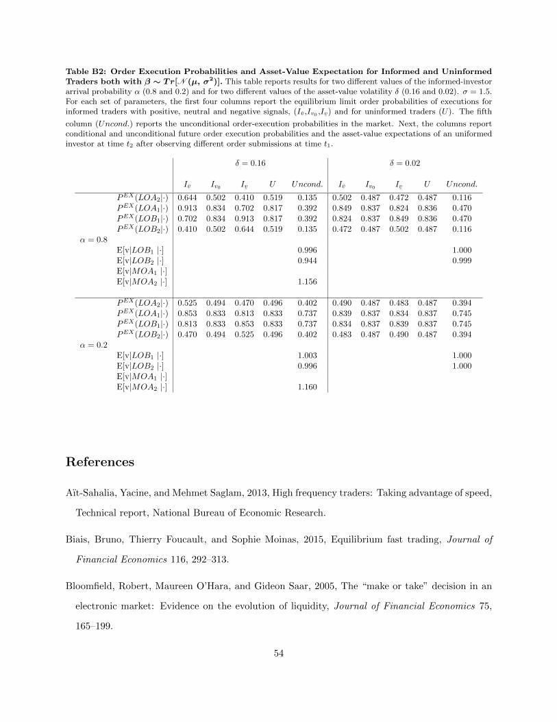
Table B2: Order Execution Probabilities and Asset-Value Expectation for Informed and UninformedTraders both with β ∼ Tr[N (µ, σ2)]. This table reports results for two different values of the informed-investorarrival probability α (0.8 and 0.2) and for two different values of the asset-value volatility δ (0.16 and 0.02). σ = 1.5.For each set of parameters, the first four columns report the equilibrium limit order probabilities of executions forinformed traders with positive, neutral and negative signals, (Iv,Iv0 ,Iv
¯) and for uninformed traders (U). The fifth
column (Uncond.) reports the unconditional order-execution probabilities in the market. Next, the columns reportconditional and unconditional future order execution probabilities and the asset-value expectations of an uniformedinvestor at time t2 after observing different order submissions at time t1.
δ = 0.16 δ = 0.02
Iv Iv0 Iv¯
U Uncond. Iv Iv0 Iv¯
U Uncond.
PEX(LOA2|·) 0.644 0.502 0.410 0.519 0.135 0.502 0.487 0.472 0.487 0.116PEX(LOA1|·) 0.913 0.834 0.702 0.817 0.392 0.849 0.837 0.824 0.836 0.470PEX(LOB1|·) 0.702 0.834 0.913 0.817 0.392 0.824 0.837 0.849 0.836 0.470PEX(LOB2|·) 0.410 0.502 0.644 0.519 0.135 0.472 0.487 0.502 0.487 0.116
α = 0.8E[v|LOB1 |·] 0.996 1.000E[v|LOB2 |·] 0.944 0.999E[v|MOA1 |·]E[v|MOA2 |·] 1.156
PEX(LOA2|·) 0.525 0.494 0.470 0.496 0.402 0.490 0.487 0.483 0.487 0.394PEX(LOA1|·) 0.853 0.833 0.813 0.833 0.737 0.839 0.837 0.834 0.837 0.745PEX(LOB1|·) 0.813 0.833 0.853 0.833 0.737 0.834 0.837 0.839 0.837 0.745PEX(LOB2|·) 0.470 0.494 0.525 0.496 0.402 0.483 0.487 0.490 0.487 0.394
α = 0.2E[v|LOB1 |·] 1.003 1.000E[v|LOB2 |·] 0.996 1.000E[v|MOA1 |·]E[v|MOA2 |·] 1.160
References
Aıt-Sahalia, Yacine, and Mehmet Saglam, 2013, High frequency traders: Taking advantage of speed,
Technical report, National Bureau of Economic Research.
Biais, Bruno, Thierry Foucault, and Sophie Moinas, 2015, Equilibrium fast trading, Journal of
Financial Economics 116, 292–313.
Bloomfield, Robert, Maureen O’Hara, and Gideon Saar, 2005, The “make or take” decision in an
electronic market: Evidence on the evolution of liquidity, Journal of Financial Economics 75,
165–199.
54
Brogaard, Jonathan, Terrence Hendershott, and Ryan Riordan, 2016, Price discovery without
trading: Evidence from limit orders.
Fleming, Michael J, Bruce Mizrach, and Giang Nguyen, 2017, The microstructure of a us treasury
ecn: The brokertec platform, Journal of Financial Markets 1–52.
Foucault, Thierry, 1999, Order flow composition and trading costs in a dynamic limit order market,
Journal of Financial Markets 2, 99–134.
Foucault, Thierry, Johan Hombert, and Ioanid Rosu, 2016, News trading and speed, Journal of
Finance 71, 335–382.
Foucault, Thierry, Ohad Kadan, and Eugene Kandel, 2005, Limit order book as a market for
liquidity, Review of Financial Studies 18, 1171–1217.
Gencay, Ramazan, Soheil Mahmoodzadeh, Jakub Rojcek, and Michael C Tseng, 2016, Price impact
and bursts in liquidity provision.
Glosten, Lawrence R, and Paul R Milgrom, 1985, Bid, ask and transaction prices in a specialist
market with heterogeneously informed traders, Journal of Financial Economics 14, 71–100.
Goettler, Ronald L, Christine A Parlour, and Uday Rajan, 2005, Equilibrium in a dynamic limit
order market, Journal of Finance 60, 2149–2192.
Goettler, Ronald L, Christine A Parlour, and Uday Rajan, 2009, Informed traders and limit order
markets, Journal of Financial Economics 93, 67–87.
Jain, Pankaj K, 2005, Financial market design and the equity premium: Electronic versus floor
trading, Journal of Finance 60, 2955–2985.
Kaniel, Ron, and Hong Liu, 2006, So what orders do informed traders use?, The Journal of Business
79, 1867–1913.
Kumar, Praveen, and Duane J Seppi, 1994, Limit and market orders with optimizing traders.
Kyle, Albert S, 1985, Continuous auctions and insider trading, Econometrica 1315–1335.
55
Milgrom, Paul, and Nancy Stokey, 1982, Information, trade and common knowledge, Journal of
Economic Theory 26, 17–27.
O’Hara, Maureen, 2015, High frequency market microstructure, Journal of Financial Economics
116, 257–270.
Parlour, Christine A, 1998, Price dynamics in limit order markets, Review of Financial Studies 11,
789–816.
Parlour, Christine A, and Duane J Seppi, 2008, Limit order markets: A survey, Handbook of
Financial Intermediation and Banking 5, 63–95.
Rindi, Barbara, 2008, Informed traders as liquidity providers: Anonymity, liquidity and price
formation, Review of Finance 497–532.
Rosu, Ioanid, 2016a, Fast and slow informed trading.
Rosu, Ioanid, 2016b, Liquidity and information in order driven markets.
56