How does latent liquidity get revealed in the limit order book?

Lorenzo Dall’Amico∗1, Antoine Fosset∗1,2, Jean-Philippe Bouchaud2, and Michael Benzaquen†1,2

1Ladhyx UMR CNRS 7646, Ecole polytechnique, 91128 Palaiseau Cedex, France2Capital Fund Management, 23 rue de l’Université, 75007, Paris, France

November 15, 2018

Abstract

Latent order book models have allowed for significant progress in our understanding of price for-mation in financial markets. In particular they are able to reproduce a number of stylized facts, such asthe square-root impact law. An important question that is raised – if one is to bring such models closerto real market data – is that of the connection between the latent (unobservable) order book and thereal (observable) order book. Here we suggest a simple, consistent mechanism for the revelation oflatent liquidity that allows for quantitative estimation of the latent order book from real market data.We successfully confront our results to real order book data for over a hundred assets and discussmarket stability. One of our key theoretical results is the existence of a market instability threshold,where the conversion of latent order becomes too slow, inducing liquidity crises. Finally we computethe price impact of a metaorder in different parameter regimes.

Introduction

In the past few years, price formation in financial markets has attracted the interest of a broad commu-nity of academics and practitioners. This can partially be explained by the growing quality of marketdata which now allows to test theories with levels of precision that have nothing to envy to naturalsciences, see e.g. [1]. The study of market impact is both of fundamental and practical relevance.Indeed, while it is an important component for understanding price dynamics, it is also the source ofsubstantial trading costs. Despite a few dissenting voices, the empirical nonlinear impact of metaorders(often coined the square root law) is now indisputably among the most robust stylized facts of modernfinance (see e.g. [2, 3, 4, 5, 6, 7, 8, 9]). In particular, for a given asset the expected average pricereturn I between the beginning and the end of a metaorder of size Q follows I(Q) = Yσd(Q/Vd)θ

where Y is a numerical factor of order one, σd and Vd denote daily volatility and daily traded volumerespectively, and θ < 1 (typically 0.4< θ < 0.6) bears witness of the concave nature of price impact.

Recently, a new class of agent based models (ABM) has helped to gain insight into the origins ofthe square root law. Given that the instantaneous liquidity revealed in the limit order book is verysmall (less than 1% of daily traded volume), latent order book models [2, 6, 10] build on the ideathat revealed liquidity chiefly reflects the activity of high frequency market makers that act as inter-mediaries between much larger unrevealed volume imbalances. The latter are not revealed in the limitorder book in order to avoid giving away precious private information, until the probability to getexecuted is large enough to warrant posting the order close to the bid (or to the ask). Within thisclass of ABM, reaction-diffusion models (see e.g. [11, 12, 13]) have proved very successful at repro-ducing the square root law in a setup free of price manipulation, and more recently consistent with

∗Both authors contributed equally to this work.†Corresponding author: michael.benzaquen@polytechnique.edu

1

arX

iv:1

808.

0967

7v2

[q-

fin.

TR

] 1

4 N

ov 2

018

the so-called diffusivity puzzle – that is, reconciling persistent order flow with diffusive price dynamics[13, 14]. However, one very important question is yet to be addressed if one is to connect such modelswith real observable and quantifiable data: what is the relation between revealed and latent liquidityand what are the mechanisms through which latent liquidity becomes revealed? These issues are thesubject of the present communication. We propose a simple dynamic model to account for liquidityflow between the latent and revealed order books. We introduce two ingredients that are to our eyesessential to reproduce realistic limit order book shapes: (i) the incentive to reveal one’s liquidity in-creases with decreasing distance to the trade price, and (ii) the process of revealing latent liquidity isnot instantaneous and lag effects may be an important source of instability, as real liquidity is found tovanish in certain regions of parameters. In addition to providing an alternative scenario for liquiditycrises, we show that our framework allows one to infer the shape of latent (unobservable) liquidityfrom real (observable) order book data. This is important because the concept of a latent order bookis sometimes criticized as a figment of the theorist’s imagination. Having more direct indications ofits existence is comforting. For an interesting discussion on the effects of liquidity timescales, see also[15] – where the authors find that the delayed revelation of latent liquidity breaks the dynamical equi-librium between the market order flow and the limit order flow, triggering large price jumps.

In section 1 we present the model and derive the governing equations. In section 2 we compute thestationary states of the limit order book both analytically and numerically. In section 3 we calibrate ourmodel to the order books of over a hundred assets and discuss market stability as function of incentiveto reveal and conversion rate. In section 4 we compute the price impact of a metaorder and discussits behavior. In section 5 we conclude.

1 A mechanism for latent liquidity revealing

Our starting point is the reaction-diffusion latent order book model of Donier et al. [12] (see also[16]). In their setup, the latent volume densities of limit orders in the order book ρB(x , t) (bid side)and ρA(x , t) (ask side) at price x and time t evolve according to the following rules. Latent orders dif-fuse with diffusivity constant D, are canceled with rate ν, and new intentions are deposited with rate λ.When a buy intention meets a sell intention they are instantaneously matched: A+B=∅. The tradeprice pt is conventionally defined through the equation ρB(pt, t) = ρA(pt, t). Donier et al. showed thatthe resulting stationary order book is locally linear (around the price). In particular, in the infinitememory limit ν,λ→ 0 while keeping L = λ/

pνD constant, one obtains ρst

A (ξ) = ρstB (−ξ) = Lξ for

ξ= x − pt > 0.1 The parameter L was coined the latent liquidity. Here we choose to work in such aninfinite memory limit. For an analysis of finite memory effects ν,λ 6= 0 see [13].

With the intention of building a mechanism for latent liquidity revealing we define the revealedand latent order books (see Fig. 1), together with the revealed and latent limit order densities forthe bid and ask sides of the book ρ(r)

A/B(x , t) and ρ(`)A/B(x , t). We denote D` and Dr the diffusion co-efficients in the latent and revealed order books respectively. Here the latent liquidity parameter isnaturally defined with respect to the latent diffusivity D`, L := λ/

p

νD` with ν,λ the cancellationand deposition rates in the latent order book (and ν,λ→ 0). While diffusion in the latent book signi-fies heterogeneous reassessments of agents intentions [12], the idea of diffusion in the revealed orderbook certainly deserves a discussion. Once a limit order is placed in the revealed order book, if onewants to change its position before it gets executed, one has to cancel it and place it somewhere else.So one may argue that there should be no diffusion in the revealed book such that revealed orderreassessments must go through the latent book before they can be posted again. However, we believethat (i) unrevealing one’s order because one is no longer confident about one’s reservation price andwaiting for an arbitrary amount of time (of order (Γωr)−1, see below) to reveal it back, and (ii) cancel-ing an order knowing that it will immediately be posted back at a revised price, are in fact two distinctprocesses. We thus leave the possibility for a nonzero diffusivity Dr in the revealed order book. Inaddition, note that trading fees and priority queues discourage traders from changing posted orders.

1Following [12] we are setting in the reference frame of the informational price component p̂t =∫ t

0ds Vs, where Vt is an

exogenous term responsible for the price moves related to common information.

2

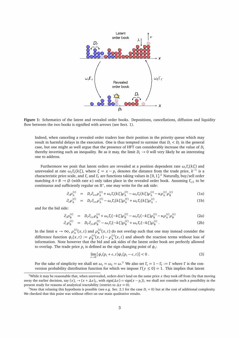
Figure 1: Schematics of the latent and revealed order books. Depositions, cancellations, diffusion and liquidityflow between the two books is signified with arrows (see Sect. 1).

Indeed, when canceling a revealed order traders lose their position in the priority queue which mayresult in harmful delays in the execution. One is thus tempted to surmise that Dr < D` in the generalcase, but one might as well argue that the presence of HFT can considerably increase the value of Drthereby inverting such an inequality. Be as it may, the limit Dr → 0 will very likely be an interestingone to address.

Furthermore we posit that latent orders are revealed at a position dependent rate ωrΓr(kξ) andunrevealed at rate ω`Γ`(kξ), where ξ = x − pt denotes the distance from the trade price, k−1 is acharacteristic price scale, and Γr and Γ` are functions taking values in [0,1].2 Naturally, buy/sell ordermatching A+ B → ∅ (with rate κ) only takes place in the revealed order book. Assuming Γr/` to becontinuous and sufficiently regular on R∗, one may write for the ask side:

∂tρ(r)A = Dr∂x xρ

(r)A +ωrΓr(kξ)ρ

(`)A −ω`Γ`(kξ)ρ

(r)A −κρ

(r)A ρ

(r)B (1a)

∂tρ(`)A = D`∂x xρ

(`)A −ωrΓr(kξ)ρ

(`)A +ω`Γ`(kξ)ρ

(r)A , (1b)

and for the bid side:

∂tρ(r)B = Dr∂x xρ

(r)B +ωrΓr(−kξ)ρ(`)B −ω`Γ`(−kξ)ρ(r)B − κρ

(r)A ρ

(r)B (2a)

∂tρ(`)B = D`∂x xρ

(`)B −ωrΓr(−kξ)ρ(`)B +ω`Γ`(−kξ)ρ(r)B . (2b)

In the limit κ →∞, ρ(r)A (x , t) and ρ(r)B (x , t) do not overlap such that one may instead consider thedifference function φr(x , t) := ρ(r)B (x , t) − ρ(r)A (x , t) and absorb the reaction terms without loss ofinformation. Note however that the bid and ask sides of the latent order book are perfectly allowedto overlap. The trade price pt is defined as the sign changing point of φr:

limε→0[φr(pt + ε, t)φr(pt − ε, t)]< 0 . (3)

For the sake of simplicity we shall set ωr = ω` = ω.3 We also set Γr = 1− Γ` := Γ where Γ is the con-version probability distribution function for which we impose Γ (y ≤ 0) = 1. This implies that latent

2While it may be reasonable that, when unrevealed, orders don’t land on the same price x they took off from (by that movingaway the earlier decision, say (x)r → (x +∆x)`, with sign(∆x) = sign(x − pt)), we shall not consider such a possibility in thepresent study for reasons of analytical tractability (restrict to ∆x = 0).

3Note that relaxing this hypothesis is possible (see e.g. Sec. 2.1 for the case Dr = 0) but at the cost of additional complexity.We checked that this point was without effect on our main qualitative results.

3

orders falling on the "wrong side" reveal themselves with rate ω. One may rightfully argue that suchorders should then be executed against the best quote, consistent with real market rules for which thereal order book cannot be crossed. However this would prevent analytical progress. We ran numericalsimulations (see section 2.3) in which such revealed orders are properly located at the best quote anddid not observe any significant impact on our main results.

Subtracting Eq. (1a) to Eq. (2a) and injecting ρ(r)B = φr1{x<pt}, ρ(r)A = −φr1{x>pt}, one obtains the

following set of equations, central to our study:

∂tρ(`)B = D`∂x xρ

(`)B −ω

¦

Γ (−kξ)ρ(`)B − [1− Γ (−kξ)]1{x<pt}φr

©

(4a)

∂tρ(`)A = D`∂x xρ

(`)A −ω

¦

Γ (kξ)ρ(`)A + [1− Γ (kξ)]1{x>pt}φr

©

(4b)

∂tφr = Dr∂x xφr +ω¦

Γ (−kξ)ρ(`)B − Γ (kξ)ρ(`)A − [1− Γ (k|ξ|)]φr

©

. (4c)

Equations (4) must be complemented with a set of boundary conditions. In particular we impose thatlimx→∞ ∂xρ

(`)A = − limx→−∞ ∂xρ

(`)B = L (see [12]), and that ρ(`)A when x → −∞, respectively ρ(`)B

when x →∞, do not diverge. In addition, whenever Dr 6= 0,4 one must impose that φr(0) = 0 andφr(x) does not diverge when |x | →∞.

2 Stationary order books

In this section we compute analytically and numerically the stationary order books as function of thedifferent parameters, and discuss interesting limit cases. Setting ∂tρ

(`)B = ∂tρ

(`)A = ∂tφr = 0 in Eqs. (4)

one obtains for all ξ ∈ R∗, ρ(`)B (ξ) = ρ(`)A (−ξ) and φr(ξ) = −φr(−ξ). This allows one to solve the

problem on R+∗, with boundary conditions ρ(`)B (0+) = ρ(`)A (0

+),∂ξρ(`)B (0

+) = −∂ξρ(`)A (0

+). The systemone must solve for ξ > 0 reduces to:

0 = D`∂ξξρ(`)B −ωρ

(`)B (5a)

0 = D`∂ξξρ(`)A −ω

¦

Γ (kξ)ρ(`)A + [1− Γ (kξ)]φr

©

(5b)

0 = Dr∂ξξφr −ω¦

Γ (kξ)ρ(`)A + [1− Γ (kξ)]φr −ρ(`)B

©

. (5c)

2.1 Analytical and numerical solutions

Here we provide a solution of Eqs. (5) for three distinct cases of interest Dr = 0, Dr = D`, and Dr 6= D`.Note that for D` = 0, one can show that ρ(`)B (ξ > 0) = 0, while φr(ξ > 0) = aξ + b with a and btwo constants, and ρ(`)A = φr[Γ (kξ)− 1]/Γ (kξ) ≈ −φr/Γ (kξ) for ξ→∞, by assuming Γ to vanish atinfinity. Such solutions are not compatible with the boundary conditions at infinity and will thereforenot be further inspected.

The limit case Dr = 0

Setting Dr = 0 in Eqs. (5) and introducing `` :=p

D`/ω, on finds that the stationary order bookdensities are given by (see Fig. 2(a)):

ρ(`)B (ξ) =

L ``2

e−ξ/`` (6a)

ρ(`)A (ξ) = Lξ+

L ``2

e−ξ/`` (6b)

φr(ξ) =L ``

2e−ξ/`` −

LξΓ (kξ)1− Γ (kξ)

. (6c)

4While Dr = 0 is an interesting limit, D` = 0 does not seem to be particularly appealing on modelling grounds. In section 2.1we give a more solid theoretical argument to support this claim.

4

Figure 2: Rescaled stationary order books as function of rescaled price for (a) Dr = 0, (b) Dr 6= D` (Dr < D`), and(c) Dr = D`. Solid black lines indicate the rescaled theoretical revealed order density kφr/L while dashed blacklines signify the theoretical latent order densities kρ(`)A/B/L . The results of the numerical simulation presented inSect. 2.3 are plotted with color lines on top of the analytical curves, with k`` = 0.35 for (a) and (c), and `r/`` = 0.32for (b). Typical computational time: 1 min.

Let us stress that the solution φr(ξ) is discontinuous in ξ = 0, consistent with no diffusion in the re-vealed order book. More precisely, provided Γ ′(0+) 6= 0, one hasφr(0−)−φr(0+) = −L [`` + 2/(Γ ′(0+)k)].While the solution for the case Dr = 0 can be expressed for an arbitrary function Γ (y > 0), this is notthe case for Dr 6= 0 and one must specify its shape. In the following we choose to work with:

Γ (y) =

�

1 ∀y ≤ 0

e−y ∀y > 0 .(7)

Note that studying the effect of a scale-invariant power law decaying Γ could also yield interestingresults.5

The limit case Dr = D`

For Dr = D` and provided k`` 6= 1 the stationary books are given by (see Fig. 2(c)):

ρ(`)B (ξ) =

Lk

g(k``)e−ξ/`` (8a)

ρ(`)A (ξ) = Lξ+

Lk

g(k``)e−ξ/`` +φr(ξ) (8b)

φr(ξ) = L�

1(k``)2 − 1

�

ξ+2k`2

`

(k``)2 − 1

�

e−kξ +g(k``)

k2``(k`` + 2)e−(1/``+k)ξ

+

�

g(k``)2k``

ξ−2k`2

`

[(k``)2 − 1]2−

g(k``)k2``(k`` + 2)

�

e−ξ/``�

, (8c)

where we introduced g(ζ) = 2ζ2(2+ ζ)2/[(1+ ζ)2(8+ 3ζ)]. For k`` = 1 the result can be obtainedby Taylor expanding Eqs. (8) about k`` = 1. Note that in this case the function φr(ξ) is continuous inξ= 0, consistent with nonzero diffusivity in the revealed order book.

5Also note that in this particular case, the solution for ω` 6= ωr can be easily expressed by substituting `` by `(r)`=p

D`/ωr

into Eqs. (6a) and (6b), and replacing Eq. (6c) by:

φr(ξ) =ωr

ω`

�

L `(r)`

2e−ξ/`

(r)` −Lξe−kξ

1− e−kξ

�

.

5

The general case Dr 6= D`

For Dr 6= D` the set of Eqs. (5) must be solved numerically. Figure 2(b) displays a plot of the stationaryorder books computed using a finite difference method for Dr/D` ≈ 0.1, that is ``/`r ≈ 3 where weintroduced `r :=

p

Dr/ω. As one can see, in the situation Dr < D` the revealed order book’s shapeis somewhat in between the cases Dr = 0 and Dr = D`, that is continuous but with a steeper slope atξ = 0. As expected, a little amount of diffusion in the revealed order book suffices to regularize thesingularity at the trade price.

As it can be seen from Eq. (5a) (or from Eqs. (6a) and (8a) in the particular cases Dr = 0 andDr = D`), in all cases `` denotes the typical scale over which the latent books overlap. This is consis-tent with the idea that `` is the typical displacement by diffusion of a latent order in the vicinity ofthe trade price during a time interval ω−1, that is before it gets revealed. Also, it can be seen fromEqs. (6c) and (8c) in the particular cases Dr = 0 and Dr = D` that the typical horizontal extension ofthe revealed order book, commonly called order book depth, is given by max(k−1,``), consistent withthe decay of the conversion probability function Γ and the horizontal extension of the latent books.Note however that, as shall be argued in Sect. 3, k−1 must always be of order or larger than `` forstability reasons, and therefore max(k−1,``) ∼ k−1. In the following we shall thus call k−1 the orderbook depth. Finally note that when `r (equivalently Dr) is decreased while keeping all other parame-ters constant, the slope of the revealed order book around the origin increases, by that concentratingfurther the available liquidity around the trade price.

2.2 The LLOB limit

Our model being built upon the locally linear order book model (LLOB) by Donier et al. [12], weshould be able to recover such a limit for certain values of the parameters. Since there is only onediffusion coefficient in the LLOB model, the latter should correspond to the Dr = D` case. Then, theLLOB model assumes no lag effect, i.e. latent orders are immediately executed when at the tradeprice. This translates intoω→∞ or equivalently ``→ 0, that is no overlap of the latent books. Morerigorously, nondimensionalizing Eqs. (8) as {φ̃r, ρ̃

(`)} = {kφr/L , kρ(`)/L} and ξ̃ = kξ, one can seethat taking the limit k`` → 0 yields for all ξ̃ > 0, ρ̃(`)B (ξ̃)→ 0, and ρ̃(`)A (ξ̃) + ρ̃

(r)A (ξ̃) = ξ̃ := ρ̃LLOB

A (ξ̃)that is precisely the LLOB result. To summarize, provided the latent order book of Donier et al. isdefined as the sum of the latent and revealed books, the LLOB limit is recovered for k`` � 1. Thelatter condition indicates that the typical displacement `` of latent orders in the vicinity of the pricemust remain small compared to the order book depth k−1. Note that, despite what a first intuitionmight suggest, the condition k →∞, that is no incentive to give away information until absolutelynecessary, is not required to recover the LLOB limit.

2.3 Numerical simulation

In order to test our results, we performed a numerical simulation of our model (see Fig. 2) whichproceeds as follows. We define four vectors ρ(`)A ,ρ(r)A ,ρ(`)B ,ρ(r)B of size 2000 on the price axis (a goodtrade-off between the continuous approximation of the model and computational time cost). Eachcomponent of vectors stores the number of orders contained at that price at a given time. At each cyclewe draw the orders that shall diffuse from a binomial distribution of parameter p`/r, directly relatedto the diffusion constant in the respective book by the relation D`/r = p`/r/(2τ) where τ denotes thetime step. Some of the orders (drawn from a binomial of parameter 1/2) will move to the left and theremaining to the right. Reflecting boundary conditions are imposed for revealed orders; the slope ofthe latent book at the boundaries is ensured by an incoming current of particles J = D`L . Then, someorders in the latent book are drawn from a binomial distribution of parameter ωτΓ (kξ) for the askside (resp. ωτΓ (−kξ) for the bid side)) and moved to the revealed book. Here pt denotes the mid-price. Equivalently revealed orders are moved to the latent book, only with parameter ωτ(1− Γ (·)).Whenever bid and ask orders are found at the same price, they are cleared from the book. Figure 2shows that the results of the numerical simulations are in very good agreement with the analyticalsolutions.

6

3 Market stability and calibration to real data

In this section, we address the important question of market stability, as given by the amount of liquidityin the revealed order book. Clearly, when the conversion rate ω is low, the revealed liquidity is thinand prices can be prone to liquidity crises, even when the latent liquidity is large. We calibrate ourmodel to real order book data and discuss the results in the light of the stability map provided by ourmodel.

3.1 Market stability

Imposing that the order densities ρ(`)A ,ρ(r)A ,ρ(`)B ,ρ(r)B must be non negative, consistent with a physicallymeaningful solution, restricts the possible values of `` :=

p

D`/ω for a given order book depth k−1.

In the Dr = 0 case, combining Eq. (6c) with Eq. (7) yields φr(0+) = L [``/2− 1/k]. Restrictingto φr(0+) ≤ 0 (which is tantamount to ρ(r)A (0

+),ρ(r)B (0+) ≥ 0) gives k`` ≤ 2. Note however that this

condition is not sufficient to say that the order densities are everywhere positive, but that they areonly positive around the origin. The necessary and sufficient condition to ensure full positivenessreads k`` ≤ 1. For 1 ≤ k`` ≤ 2 the order book displays a "hole" along the price axis, but is welldefined around the origin. Since we are most interested in the revealed liquidity in the vicinity of thetrade price we will choose k`` ≤ 2 (or, in terms of ω, ω ≥ D`k

2/4) as our stability condition, with noqualitative and only little quantitative effect on our main conclusions. The maximum amplitude of thereal order book density scales as:

maxξ

�

�φr(ξ)�

�= −φr(0+) =

Lk

�

1−k``ζc

�

, ζc = 2 . (9)

For D` = Dr the stability condition is imposed by the sign of the slope at ξ = 0. One finds that thecritical value of k`` for which the liquidity around the origin vanishes is given by ζc = [−2 + (73 −6p

87)1/3+(73+6p

87)1/3]/3≈ 1.875.6 Arguing that in this case the maximum of the density can beapproximated by maxξ

�

�φ′r(0+)ξe−kξ

�

�= |φ′r(0+)|/(ek) yields:

maxξ

�

�φr(ξ)�

�∼Lek

ζc(3ζ2c + 4ζc − 3)

(1+ ζc)2(8+ 3ζc)

�

1−k``ζc

�

, ζc ≈ 1.875 . (10)

Figure 3(a) displays −kφ′r(0+)/L as function of the dimensionless parameters k`` and k`r. The

dash-dotted line corresponding to φ′r(0) = 0 splits the parameter space into a stable region (green)and an unstable region (red). We naturally checked that the analytical values of ζc obtained abovefor `` = `r and `r → 0 are recovered. As one can see, while the role played by `r with respect to theposition of the critical line ζc is quite marginal (quasi-vertical dash dotted line), the slope of the orderbook around ξ= 0 increases with decreasing `r/``. More precisely, Fig. 3(c) displays the slope of therevealed book in the vicinity of the transition and shows that, at given `r/``, the slope indeed scaleslinearly with |k`` − ζc|. In addition the top right inset shows that the slope also scales as ``/`r, whichfinally leads to |φ′r(0

+)| ∼ |k``−ζc|(``/`r). The other insets show ζc as function of `r/``, and the totalrevealed volume. For the sake of completeness, Fig. 3(b) displays a proxy of the overlap between thelatent bid and ask books in the parameter space (k``, k`r). While vanishing in the region k``� ζc, theoverlap is quite large (of the order of k−1) in the vicinity of the critical line k`` ® ζc indicating a largevolume of latent orders in the vicinity of the price. Interestingly, combined with a vanishing level ofliquidity, the increased level of activity around the origin induces important fluctuations of the tradeprice. To illustrate this, Fig. 3(d) displays the numerically determined squared volatility of the tradeprice pt as function of k`` in the `r = `` limit. For comparison, we also plotted the volatility of the fairprice pf

t , here defined as the value that equilibrates total (revealed and latent) supply and demand:

∫ pft

0

dξ�

ρ(r)A (ξ, t) +ρ(`)A (ξ, t)

�

=

∫ ∞

pft

dξ�

ρ(r)B (ξ, t) +ρ(`)B (ξ, t)

�

. (11)

6Note that in this case the solution, provided k`` > 1, is also asymptotically unstable: limξ→∞φr(ξ) =L g(k``)ξe−ξ/``/(2k``)> 0, while for k`` = 1, limξ→∞φr < 0.

7

Figure 3: Parametric study of stationary order books. (a) Stability map. Density plot (symlog scale) of the rescaledslope of the revealed order density at the origin, as function of k`` and k`r. The dashed line indicates `r = ``, thedash-dotted line indicates the critical line φ′r(0) = 0. (b) Overlap of the latent order books. Density plot (log scale)of the y-intercept of the latent order book densities at the origin. Note that such a quantity is a direct measure of theoverlap. Typical computational time to draw the stability map: 1 h. The empirical order book data (US stocks, seeTab. 1, and Euro Stoxx, white star) are reported with a colormap scaling with their average spread value (see (a))and with their average daily traded volume (see (b)). The light blue star results from the calibration of Euro Stoxxdata 2h around the flash crash of February 5th 2018 at 8:15pm (Paris time). Typical computational time: 1 min foreach asset. (c) Plot of the slope of the revealed order book at the origin as function of ζc−k``, for different values of`r/``. The top inset shows ζc as function of `r/``, and the center left inset displays the total volume in the revealedorder book Vr =

�

�

∫∞0 dξφr(ξ)1φr(ξ)<0

�

�, as function of ζc− k``. The right inset shows the angular coefficient of theslope of the main plot at the origin. (d) Numerical volatility. Plot of rescaled numerical squared volatility of the tradeprice and the fair price (see Eq. (11)) in the `r = `` case. We display two different estimations: Rogers-Satchell,σ2

RS = E [(pH − pO)(pH − pC) + (pL − pO)(pL − pC)], and Parkinson, σ2p =

14 ln(2)E

�

(pH − pL)2�

where pH, pL, pO, pC

denote the high, low, open and close prices respectively [17, 18].

As one can see, for ω � ωc := D`k2/ζ2

c the volatility of the trade price coincides with its fair pricecounterpart, consistent with the idea that for high conversion rates the coupling between the revealedand latent books is almost instantaneous and therefore the mid-price tends to follow the fair price. Inthe vicinity of the critical line the volatility of the fair price slightly decreases. However, the volatil-ity of the trade price strongly diverges as the vanishing liquidity limit is approached, i.e. when theconversion rate ω decreases to ωc. Note that while the trade price can no longer be defined when aliquidity crisis arises, the fair price as defined in Eq. (11) remains well behaved. We also investigated

8

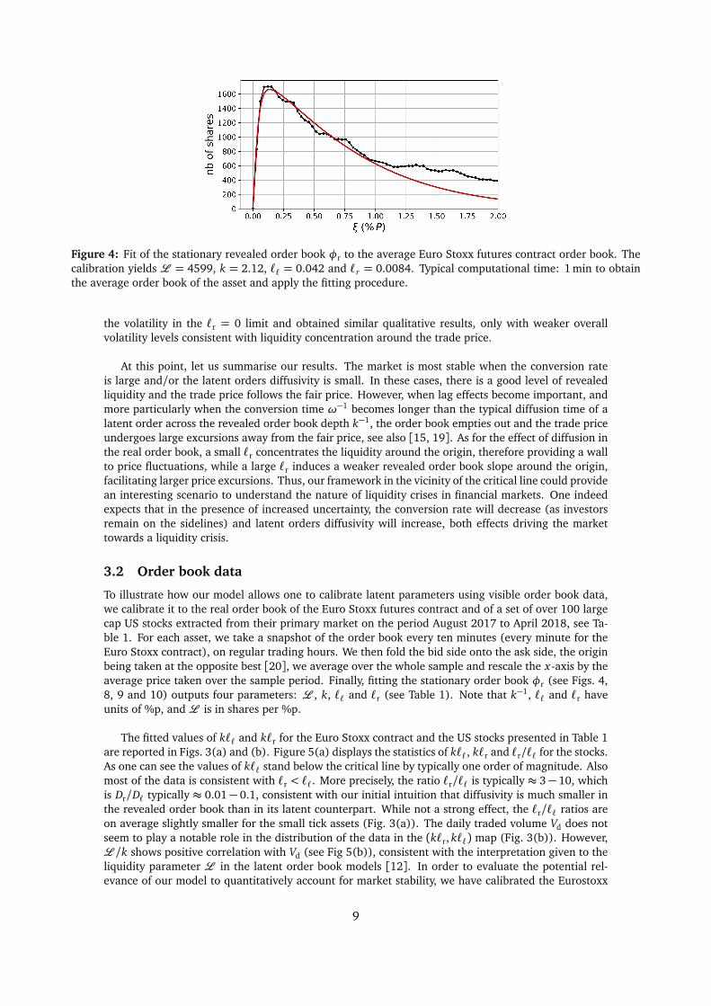
Figure 4: Fit of the stationary revealed order book φr to the average Euro Stoxx futures contract order book. Thecalibration yields L = 4599, k = 2.12, `` = 0.042 and `r = 0.0084. Typical computational time: 1 min to obtainthe average order book of the asset and apply the fitting procedure.

the volatility in the `r = 0 limit and obtained similar qualitative results, only with weaker overallvolatility levels consistent with liquidity concentration around the trade price.

At this point, let us summarise our results. The market is most stable when the conversion rateis large and/or the latent orders diffusivity is small. In these cases, there is a good level of revealedliquidity and the trade price follows the fair price. However, when lag effects become important, andmore particularly when the conversion time ω−1 becomes longer than the typical diffusion time of alatent order across the revealed order book depth k−1, the order book empties out and the trade priceundergoes large excursions away from the fair price, see also [15, 19]. As for the effect of diffusion inthe real order book, a small `r concentrates the liquidity around the origin, therefore providing a wallto price fluctuations, while a large `r induces a weaker revealed order book slope around the origin,facilitating larger price excursions. Thus, our framework in the vicinity of the critical line could providean interesting scenario to understand the nature of liquidity crises in financial markets. One indeedexpects that in the presence of increased uncertainty, the conversion rate will decrease (as investorsremain on the sidelines) and latent orders diffusivity will increase, both effects driving the markettowards a liquidity crisis.

3.2 Order book data

To illustrate how our model allows one to calibrate latent parameters using visible order book data,we calibrate it to the real order book of the Euro Stoxx futures contract and of a set of over 100 largecap US stocks extracted from their primary market on the period August 2017 to April 2018, see Ta-ble 1. For each asset, we take a snapshot of the order book every ten minutes (every minute for theEuro Stoxx contract), on regular trading hours. We then fold the bid side onto the ask side, the originbeing taken at the opposite best [20], we average over the whole sample and rescale the x-axis by theaverage price taken over the sample period. Finally, fitting the stationary order book φr (see Figs. 4,8, 9 and 10) outputs four parameters: L , k, `` and `r (see Table 1). Note that k−1, `` and `r haveunits of %p, and L is in shares per %p.

The fitted values of k`` and k`r for the Euro Stoxx contract and the US stocks presented in Table 1are reported in Figs. 3(a) and (b). Figure 5(a) displays the statistics of k``, k`r and `r/`` for the stocks.As one can see the values of k`` stand below the critical line by typically one order of magnitude. Alsomost of the data is consistent with `r < ``. More precisely, the ratio `r/`` is typically ≈ 3− 10, whichis Dr/D` typically ≈ 0.01− 0.1, consistent with our initial intuition that diffusivity is much smaller inthe revealed order book than in its latent counterpart. While not a strong effect, the `r/`` ratios areon average slightly smaller for the small tick assets (Fig. 3(a)). The daily traded volume Vd does notseem to play a notable role in the distribution of the data in the (k`r, k``) map (Fig. 3(b)). However,L /k shows positive correlation with Vd (see Fig 5(b)), consistent with the interpretation given to theliquidity parameter L in the latent order book models [12]. In order to evaluate the potential rel-evance of our model to quantitatively account for market stability, we have calibrated the Eurostoxx

9

Figure 5: (a) Histograms of the fitted parameters k``, k`r and `r/`` for the US stocks presented in Table 1. (b)Average daily traded volume Vd as function of the liquidity parameterL /k. The data points are coloured by density(from yellow to dark blue).

data on a particularly agitated subset, that is the two hours about the flash crash of February 5th 2018at 8:15pm (Paris time), see light blue star on pannels (a) and (b) of Fig. 3. One finds, as expected,that the new data point is closer to the critical line than the reference point (white star), indicatinglesser stability during the flash crash period.

4 Price impact

In this section we study how liquidity reacts, in our model, to the presence of a metaorder, namelya large trading order split into small orders executed incrementally. Following Donier et al. [12] weintroduce a metaorder as an additional current of buy/sell particles falling precisely at the trade price.The system of equations governing the system in the presence of a metaorder is left unchanged forthe latent order book (Eqs. (4a) and (4b)), while the RHS of Eq. (4c) must be complemented withthe extra additive term + mtδ(x − pt), representing the metaorder, with mt the execution rate andδ the Dirac delta function. In the following we restrict to buy metaorders with constant executionrates mt = m0 > 0, without loss of generality since the sell metaorder m0 < 0 is perfectly symmetric.In order to extract the dimensionless parameters governing the dynamic system, we introduce ξ̃ =kξ, t̃ =ωt, ρ̃ = kρ/L , φ̃r = kφr/L and write the equations in a dimensionless form:

∂ t̃ ρ̃(`)B = (k``)

2∂ x̃ x̃ ρ̃(`)B −

¦

Γ (−ξ̃)ρ̃(`)B − [1− Γ (−ξ̃)]1{ x̃<p̃ t̃}φ̃r

©

(12a)

∂ t̃ ρ̃(`)A = (k``)

2∂ x̃ x̃ ρ̃(`)A −

¦

Γ (ξ̃)ρ̃(`)A + [1− Γ (ξ̃)]1{ x̃>p̃ t̃}φ̃r

©

(12b)

∂ t̃φ̃r = (k`r)2∂ x̃ x̃ φ̃r −

¦

Γ (ξ̃)ρ̃(`)A − Γ (−ξ̃)ρ̃(`)B + [1− Γ (|ξ̃|)]φ̃r

©

+ (m0/J )δ(ξ̃) , (12c)

with J =Lω/k2 the typical scale of the rate at which latent orders are revealed (recall that L /k2 isthe typical available volume in the latent order book that have a substantial probability to be revealed).Matching the first and third terms on the right hand side of Eq. (12c) yields a relevant dimensionlessnumber (m0/J )/(k`r)2 = m0/Jr with Jr = DrL . In the case `r = 0 the relevant dimensionless numberis simply given by m0/J .

In order to compute the price impact I(Q t) = E[pt − p0|Q t = m0 t], we performed numerical sim-ulations of our model in the presence of a metaorder in several limit cases. More specifically, startingfrom the stationary order books, we implemented a buy/sell metaorder as an additional current ofbuy/sell particles falling precisely at the best ask/bid, thus acting as a sequence of market orders. Westored the order books as a function of time to be able to compute dynamically the relevant scalarquantities below. We explored in particular `r = `` and `r = 0, in both high and low participation rateregimes, for different values of k`` (see Figs. 6 and 7).

Before presenting the results of the numerical simulations, note that there exists a regime wherethe calculations can be brought a little bit further analytically, that is when we can give a geometricalinterpretation to the problem. When the book is almost static on the time scale of the metaorder

10

Figure 6: Price impact for `r = ``. (a) m0 � Jr (b) m0 � Jr. The dashed green lines indicate the LLOB limits,ILLOB(t) =

p

αQ t/(πL ) with α = m0/Ju for the slow regime and ILLOB(t) =p

2Q t/L for the fast regime. The topleft insets on each plot indicate the factor c as function of k`` defined as I(t) = c ILLOB(t). The top right inset ofsubplot (a) shows an extreme regime with very high execution rate, the dash-dotted line indicates the theoreticalprediction as given by the numerical inversion of Eq. (14). Subplots (c) and (d) display relative price differencebetween the trade price and the fair price (see Eq. (11)). Subplots (e) and (f) display the relative revealed volumeimbalance. Typical computational time: a few hours to obtain all the impact curves.

execution i.e. m0� Jr (resp. m0�J for `r = 0), one has∫ t

0 ds m0 = −∫ pt

0 dξφstr (ξ) with ξ= x − p0.

In particular for `r = 0 one obtains:

Q t = −L `2

`

2

�

1− e−pt/``�

+L pt

klog

�

1− e−kpt�

−Lk2

�

Li2(e−kpt)− Li2(1)

�

, (13)

where Li2(y) =∑∞

k=1 yk/k2 stands for the polylogarithm of order 2, and can be inverted numericallyto obtain the price trajectory pt . Similarly, for `r = `` one has:

Q t =Lαk2

�

[k(pt + β) + 1]e−kpt − (kβ + 1)

−L ``γ

1+ k``

�

1− e−(k+1/``)pt�

+ L ``ηpt e−pt/`` −L [η`2

` − ``(αβ + γ)]�

1− e−pt/``�

, (14)

where α = [(k``)2 − 1]−1, β = 2αk`2`, γ = g(k``)[k2``(k`` + 2)]−1, η = g(k``)[2k``]−1. In the

following we discuss the more general numerical results for both limit cases `` = `r and `r = 0.

The case `` = `r

The main plots in Figs. 6(a) and (b) display robust square root price trajectories, regardless of thevalues of k``. For m0� Jr the price trajectory matches the theoretical prediction given above inverting

11

Eq. (14). As expected from the exponentially vanishing liquidity when x−p0 > k−1, impact eventuallydiverges for very extreme regimes, see top right inset in Fig. 6(a). For k``� 1, one recovers the LLOBlimit in both fast and slow regimes, also as expected. For non vanishing values of k``, the impactincreases with increasing k``. In particular for m0� Jr one obtains at short times (equivalently smallvolumes):

pt =

√

√ 2Q t

|∂xφr(0+)|∼p

2Q t

�

1−k``ζc

�−1/2

. (15)

As expected, impact diverges when at the incipient liquidity crisis point. Figures 6(c) and (d) displaythe relative distance between the trade price and the fair price as function of time. In the fast executionregime all curves fall on top of each other and |pt − pf

t | ≈ |pt |, consistent with the idea that the book(in particular latent) does not have time to reassess during the execution, and as a consequence thefair price varies at a much slower rate than the trade price. A different scenario takes place in the smallexecution rate regime. We observe that the relative distance between trade and fair prices stabilizes.In other terms, the latent order book evolves at a speed that is comparable to that of the metaorderand the fair price follows the trade price quite accurately.

The evolution of relative volume imbalance (see Figs. 6(e) and (f)) allows one to draw similarconclusions. In the fast execution limit, the imbalance diverges as the latent order book has no time torefill the revealed order book (this effect is all the more evident as we approach the vanishing liquiditylimit k`` → ζc), while in the slow execution limit the imbalance is much smaller. Most importantly,note that in this limit the imbalance becomes positive. This is consistent with the fact that when thetrade price moves slowly, the conversion probability Γ is shifted with it and new orders reveal on topof the existing ones to supply the metaorder, while the orders left behind progressively unreveal.

The case `r = 0

The limit `r → 0 corresponds to m0/Jr →∞, so in some sense one could say that we are always ina high participation rate regime. However the absence of diffusion means that the system can onlyevolve through the revealing and unrevealing currents. As mentioned above, in this case the relevantdimensionless number becomes m0/J , that shall be referred to as participation rate in the following.

Figure 7(a) displays price trajectories in the fast execution regime, here m0 �J . The metaorderis faster than the revealing current and the price trajectory is given by inverting Eq. (13). At shorttimes, one obtains (see Eq. (9)):

pt =kQ t

L

�

1−k``ζc

�−1

, (16)

which is linear impact, consistent with φr(0) 6= 0. Analogous to the case `` = `r, in extreme regimesthe impact eventually diverges (see top right inset of Fig. 7(a)). Regarding the imbalance and the rel-ative distance between the trade price and the fair price, the interpretation is analogous to the `r = ``case.

Figure 7(b) displays the price trajectories in the low participation rate regime m0 �J . Here theimpact is genuinely linear at short times but crossovers to concave after a typical time t? ∼ Vr/m0 withVr the typical volume available in the revealed order book. This interesting regime can be easily under-stood as follows. At short times the metaorder is executed against the orders present in the stationarylocally constant revealed order book (linear impact), but after a while liquidity revealing from thelinear latent order book takes over (implying concave impact).7 More precisely, as k`` is increased, t?

is decreased consistent with the idea that: the larger k``, the smaller the revealed liquidity Vr and thusthe sooner it gets consumed. Note that linear impact at short times (equiv. small volumes) has beenreported empirically in the literature [21]. An alternative theoretical framework to understand linearimpact at short times is provided in [13] with the introduction of two types of agents, fast and slow.Our model, in its final version, should also include the possibility for agents with different timescales,

7Note that recovering precisely the square root law in this regime is quite challenging because the numerical simulation, byessence discontinuous, induces artificial spread effects: the spread widens and does not get refilled as fast as it should, due tolimited resolution and vanishing liquidity in the price region. Obtaining smooth results requires a lot of averaging.

12

Figure 7: Price impact for `r = 0. (a) and m0 � J (b) m0 � J . The top left insets on subplot (a) indicatesthe factor c as function of k`` here defined as I(t) = c t for `r = 0. The top right insets show an extreme regimewith very high execution rate for which the impact diverges. Subplots (c) and (d) display relative price differencebetween the trade price and the fair price, see Eq. (11). Subplots (e) and (f) display the relative revealed volumeimbalance. Typical computational time: a few hours to obtain all the impact curves.

possibly with different conversion rates ω. In Fig. 7(d), we observe that the relative distance betweentrade and fair prices stabilizes after the typical time t?. In other terms, for t > t? the latent order bookevolves at a rate comparable to that of the metaorder, and the fair price follows the trade price withsome constant lag. Figure 7(f) displays similar conclusions.

5 Concluding remarks

We have proposed a simple, consistent model describing how latent liquidity gets revealed in the realorder book. As a first step in the rapprochement of latent order book models and real order book data,our study upgrades the former from a toy model status to an observable setup that can be quantita-tively calibrated on real data. Although probably too simple in its present form, our main contributionis to show how the latent order book could be inferred from its revealed counterpart. One of our keytheoretical result is the existence of a market instability threshold, where the conversion of the trad-ing intentions of market participants into bona fide limit orders becomes too slow, inducing liquiditycrises. From a regulatory perspective, our model indicates how assets can be sorted according to theirposition in the stability map, a proxy for their propensity to liquidity dry-ups and large price jumps. Inparticular, our setup could constitute an insightful alternative to relate stability and tick size, a subjectthat has raised the attention of many in the recent past (see e.g. [22]). To confirm potential perspec-tives for market regulation, we showed that our model exhibits lesser stability when calibrating thesame asset during a period of higher volatility.

13

While providing quite satisfactory results on several grounds, our model lacks a number of featuresthat must be addressed in future work. In particular, being an inheritance of the LLOB model [12], ourmodel does not solve the so-called diffusivity puzzle (even persistent order flow lead to mean-revertingprices – see [6, 14, 13]). An interesting extension is suggested by the stocks data presented in Figs 8,9 and 10. Indeed, some of the order books display a bimodal shape indicating that they would bebetter fitted with a model involving two conversion timescales (equivalently two price scales). The re-cent multi-timescale liquidity setup (see [13]) allows for both a fast liquidity of high frequency marketmakers, and a slow liquidity of directional traders, while resolving several difficulties of latent orderbook models. Such a framework should output bimodal distributions and yield even better fits of thereal order book, allowing one to infer different liquidity timescales.

We thank Frédéric Bucci, Alexandre Darmon, Jonathan Donier, Stephen Hardiman and IacopoMastromatteo for fruitful discussions.

References

[1] Kanazawa K, Sueshige T, Takayasu H and Takayasu M 2018 Physical review letters 120 138301

[2] Tóth B, Lemperiere Y, Deremble C, De Lataillade J, Kockelkoren J and Bouchaud J P 2011 PhysicalReview X 1 021006

[3] Torre N 1997 BARRA Inc., Berkeley

[4] Almgren R, Thum C, Hauptmann E and Li H 2005 Risk 18 5862

[5] Engle R, Ferstenberg R and Russell J 2006

[6] Mastromatteo I, Tóth B and Bouchaud J P 2014 Physical Review E 89 042805

[7] Brokmann X, Serie E, Kockelkoren J and Bouchaud J P 2015 Market Microstructure and Liquidity1 1550007

[8] Bacry E, Iuga A, Lasnier M and Lehalle C A 2015 Market Microstructure and Liquidity 1 1550009

[9] Bershova N and Rakhlin D 2013 Quantitative finance 13 1759–1778

[10] Lehalle C A, Guéant O and Razafinimanana J 2011 High-frequency simulations of an order book:a two-scale approach Econophysics of Order-driven Markets (Springer) pp 73–92

[11] Bak P, Paczuski M and Shubik M 1997 Physica A: Statistical Mechanics and its Applications 246430–453

[12] Donier J, Bonart J F, Mastromatteo I and Bouchaud J P 2015 Quantitative Finance 15 1109–1121

[13] Benzaquen M and Bouchaud J P 2018 Quantitative Finance 1–10

[14] Benzaquen M and Bouchaud J P 2018 The European Physical Journal B 91 23

[15] Corradi F, Zaccaria A and Pietronero L 2015 Physical Review E 92 062802

[16] Smith E, Farmer J D, Gillemot L s, Krishnamurthy S et al. 2003 Quantitative finance 3 481–514

[17] Rogers L C, Satchell S E and Yoon Y 1994 Applied Financial Economics 4 241–247

[18] Parkinson M 1980 Journal of business 61–65

[19] Cristelli M, Alfi V, Pietronero L and Zaccaria A 2010 The European Physical Journal B 73 41–49

[20] Bouchaud J P, Bonart J, Donier J and Gould M 2018 Trades, quotes and prices: financial marketsunder the microscope (Cambridge University Press)

[21] Zarinelli E, Treccani M, Farmer J D and Lillo F 2015 Market Microstructure and Liquidity 11550004

[22] Dayri K and Rosenbaum M 2015 Market Microstructure and Liquidity 1 1550003

14

Figure 8: Fit of the stationary revealed order book φr to the average order books of over one hundred US stocks,see Table 1. 15

Figure 9: Fit of the stationary revealed order book φr to the average order books of over one hundred US stocks,see Table 1. 16

Figure 10: Fit of the stationary revealed order book φr to the average order books of over one hundred US stocks,see Table 1. 17

Stock price $ S 10−6Vd 10−3L k `` `r

RIMM 10.03 1.003 0.87 602.0 4.71 0.0020 0.0059BAC 28.66 1.007 15.62 34.3 2.50 0.0350 0.0033AGNC 19.92 1.009 1.03 10.8 2.51 0.0165 0.0005VOD 29.62 1.011 0.89 47.6 5.58 0.0230 0.0090CSCO 38.57 1.012 7.17 26.7 3.64 0.0309 0.0027CY 16.14 1.018 1.44 11.9 2.49 0.0195 0.0020ABX 16.46 1.023 2.95 191.1 4.45 0.0031 0.0060CMCSA 37.65 1.023 6.54 38.3 6.31 0.0230 0.0046SBC 36.51 1.029 7.76 5.3 1.75 0.0417 0.0023KFT 42.25 1.036 2.88 39.1 10.22 0.0131 0.0047FCX 16.45 1.040 4.74 8.3 2.22 0.0201 0.0054INTC 44.87 1.042 8.31 16.7 3.31 0.0318 0.0024PBR 13.54 1.044 4.59 16.9 1.99 0.1284 0.0035EBAY 39.12 1.052 2.73 28.1 7.71 0.0176 0.0037SYMC 28.96 1.072 1.78 19.4 5.50 0.0227 0.0040GSK 37.99 1.074 0.83 38.4 10.94 0.0084 0.0069SBUX 57.01 1.076 2.95 9.4 4.53 0.0178 0.0009WFC 56.31 1.082 5.37 25.6 11.02 0.0156 0.0057NWS 33.21 1.100 2.55 18.7 5.74 0.0262 0.0065DISCA 22.57 1.101 1.42 13.7 4.46 0.0247 0.0072BEL 49.35 1.104 4.09 10.0 6.11 0.0278 0.0048FD 23.44 1.117 2.46 3.9 2.26 0.0411 0.0093BBBY 22.20 1.118 1.35 7.0 3.17 0.0178 0.0008SO 44.21 1.143 1.69 5.2 4.87 0.0323 0.0060GT 31.36 1.191 0.98 17.8 7.24 0.0169 0.0035MRK 56.76 1.210 3.54 11.5 9.16 0.0209 0.0071XOM 80.51 1.219 4.03 11.2 8.03 0.0231 0.0042C 73.26 1.225 5.28 8.8 6.83 0.0261 0.0040HAL 47.17 1.254 2.35 28.7 11.94 0.0117 0.0097URBN 23.44 1.257 0.92 10.5 4.57 0.0123 0.0007VIA 29.54 1.264 1.66 14.2 6.45 0.0127 0.0020AMAT 53.43 1.315 3.53 5.6 3.23 0.0305 0.0021PG 84.03 1.401 2.60 30.7 17.95 0.0098 0.0078QCOM 59.38 1.416 3.30 4.0 3.25 0.0177 0.0006MO 64.07 1.428 2.09 14.9 13.02 0.0143 0.0064DOW 64.99 1.439 2.35 100.6 25.26 0.0015 0.0030P 52.99 1.439 1.85 17.5 11.15 0.0149 0.0104CSX 54.49 1.561 2.16 9.8 6.77 0.0199 0.0026NKE 63.01 1.586 2.29 12.4 10.24 0.0191 0.0088AIG 61.12 1.592 1.48 15.9 12.27 0.0168 0.0109GIS 49.88 1.645 1.17 1.3 2.79 0.0431 0.0037SLB 67.36 1.661 2.20 14.9 11.92 0.0167 0.0097CMB 106.81 1.667 4.03 8.6 11.14 0.0199 0.0048MYL 39.10 1.748 1.98 16.1 8.65 0.0184 0.0049STX 45.28 1.822 1.48 4.6 4.09 0.0212 0.0013WMT 90.73 1.884 2.59 8.3 10.61 0.0211 0.0055AAPL 168.14 1.922 8.78 3.1 2.51 0.0107 0.0011OXY 64.65 1.971 1.20 9.6 10.77 0.0191 0.0101BMY 61.12 2.032 1.76 1.5 4.21 0.0372 0.0044CTSH 75.94 2.129 1.27 23.7 17.41 0.0095 0.0040LOW 81.69 2.204 1.61 6.9 11.71 0.0194 0.0078WAG 71.64 2.298 2.25 10.3 9.79 0.0176 0.0032HOLX 42.09 2.314 0.88 317.2 29.35 0.0008 0.0012TGT 66.76 2.409 1.53 2.4 5.62 0.0320 0.0050DIS 103.38 2.440 2.36 5.4 9.51 0.0236 0.0057FAST 50.13 2.495 0.91 5.9 6.68 0.0213 0.0032YHOO 71.07 2.649 2.55 21.6 8.05 0.0042 0.0043DISH 48.54 2.671 0.82 3.3 5.53 0.0309 0.0059HANS 59.37 2.751 0.84 13.8 11.79 0.0163 0.0047GLNG 27.57 2.925 0.35 14.1 7.52 0.0187 0.0048PEP 112.52 3.009 1.42 5.3 8.42 0.0174 0.0020ESRX 69.15 3.032 1.45 9.6 11.69 0.0137 0.0029CERN 67.81 3.100 0.81 13.6 13.42 0.0134 0.0037TXN 99.90 3.131 1.82 4.6 7.61 0.0200 0.0025

Stock price $ S 10−6Vd 10−3L k `` `r

ROST 70.66 3.149 1.06 6.2 8.32 0.0198 0.0033CREE 34.92 3.165 0.51 2.0 3.48 0.0322 0.0030XLNX 70.21 3.199 0.93 4.0 7.34 0.0200 0.0026CHV 116.12 3.867 1.95 16.8 19.58 0.0085 0.0108IBM 152.11 3.917 1.29 3.9 11.96 0.0218 0.0083CHRW 87.75 3.980 0.59 41.7 22.18 0.0075 0.0034JNJ 131.86 4.007 2.07 6.9 15.56 0.0149 0.0098MYGN 33.28 4.032 0.31 61.1 17.84 0.0019 0.0021MCD 156.99 4.131 1.07 3.5 10.38 0.0276 0.0109V 121.14 4.170 2.20 1.0 5.21 0.0381 0.0058FISV 106.11 4.408 0.43 377.8 36.42 0.0008 0.0010UPS 107.88 5.055 0.87 0.4 3.02 0.0566 0.0071DLTR 97.27 5.124 0.86 2.0 6.07 0.0206 0.0019CRM 116.98 5.563 1.22 0.5 4.61 0.0452 0.0074HON 148.04 5.754 0.78 1.4 7.36 0.0365 0.0151ERTS 116.94 5.872 1.07 220.6 34.96 0.0101 0.0641HD 175.53 5.944 1.35 2.4 9.83 0.0275 0.0079CHKP 104.95 6.161 0.38 1.3 7.57 0.0183 0.0020CTAS 161.47 6.443 0.25 141.6 38.58 0.0038 0.0040EXPE 124.49 6.716 0.83 0.8 4.82 0.0114 0.0006CAT 153.78 6.934 1.10 1.2 6.78 0.0408 0.0106ADSK 118.11 6.967 0.77 0.8 4.34 0.0181 0.0010GS 230.09 6.976 0.76 30.5 27.22 0.0011 0.0038DE 154.44 6.985 0.58 1.6 8.70 0.0338 0.0216FFIV 128.76 7.457 0.30 4.9 15.98 0.0095 0.0016AMGN 179.67 7.504 1.31 0.5 3.42 0.0187 0.0009JAZZ 146.67 8.266 0.14 5.6 12.72 0.0064 0.0007BRK 202.45 8.669 1.34 2.1 12.53 0.0257 0.0107INCY 97.51 8.723 0.64 2.2 9.68 0.0095 0.0007MMM 222.45 8.976 0.70 1.4 9.74 0.0334 0.0167WYNN 162.67 9.496 0.76 0.2 2.17 0.0106 0.0004ALXN 122.92 9.738 0.69 0.9 6.73 0.0154 0.0013WPI 176.75 10.580 0.70 0.1 3.37 0.0575 0.0093BA 297.60 10.630 0.97 0.2 3.31 0.0404 0.0037VRTX 155.65 11.509 0.56 1.0 8.18 0.0105 0.0009EQIX 433.69 11.889 0.20 2.3 12.98 0.0015 0.0002FDX 246.89 12.048 0.36 0.4 7.53 0.0445 0.0183ORLY 224.90 12.416 0.43 0.8 8.09 0.0119 0.0009REGN 372.48 12.480 0.30 3.4 16.62 0.0028 0.0002ILMN 217.03 12.989 0.34 0.7 7.93 0.0178 0.0033CHTR 344.48 13.312 0.67 0.9 8.88 0.0060 0.0005IDPH 307.01 13.479 0.54 0.8 9.68 0.0099 0.0014AMZN 1097.54 14.080 1.34 160.6 31.19 0.0117 0.2002GOOG 1009.80 14.339 0.66 0.2 5.03 0.0009 0.0001

Table 1: US stocks (large cap.) used for the empiricalanalysis of Sec. 3.2 (see also Figs. 8, 9 and 10). The aver-age spread S has tick units, Vd denotes the average dailytraded volume (in shares), k−1, `` and `r are expressedin %price, and L is shares per unit %price.

18