information contagion and systemic risk - bank of …...2 bank of canada staff working paper 2017-29...

Bank of Canada staff working papers provide a forum for staff to publish work-in-progress research independently from the Bank’s Governing Council. This research may support or challenge prevailing policy orthodoxy. Therefore, the views expressed in this paper are solely those of the authors and may differ from official Bank of Canada views. No responsibility for them should be attributed to the Bank.

www.bank-banque-canada.ca

Staff Working Paper/Document de travail du personnel 2017-29

Information Contagion and Systemic Risk

by Toni Ahnert and Co-Pierre Georg

2

Bank of Canada Staff Working Paper 2017-29

July 2017

Information Contagion and Systemic Risk

by

Toni Ahnert1 and Co-Pierre Georg2

1Financial Stability Department Bank of Canada

Ottawa, Ontario, Canada K1A 0G9 [email protected]

2Research Department Deutsche Bundesbank

and University of Cape Town

Rondebosch, Cape Town, South Africa [email protected]

ISSN 1701-9397 © 2017 Bank of Canada

mailto:[email protected]

mailto:[email protected]

i

Acknowledgements

The authors wish to thank Viral Acharya, Jose Berrospide, Falko Fecht, Douglas Gale,

Prasanna Gai (discussant), Paul Glassermann (discussant), Itay Goldstein, Todd Keister,

Anton Korinek, Yaron Leitner, Ralf Meisenzahl, Jean-Charles Rochet, Cecilia Parlatore

Siritto, Javier Suarez, Ernst-Ludwig von Thadden, Dimitri Vayanos, Tanju Yorulmazer, and

seminar participants at the IMF, LSE, NYU and the Philadelphia Fed, and conference

participants at the RBNZ-UA "Stability and Efficiency of Financial Systems" conference,

the 2012 FDIC Bank Research Conference, and EEA 2011 meeting for fruitful discussions

and comments. These are the views of the authors and do not necessarily reflect the

views of the Bank of Canada or Deutsche Bundesbank. All remaining errors are our own.

ii

Abstract

We examine the effect of ex-post information contagion on the ex-ante level of systemic

risk defined as the probability of joint bank default. Because of counterparty risk or

common exposures, bad news about one bank reveals valuable information about

another bank, triggering information contagion. When banks are subject to common

exposures, information contagion induces small adjustments to bank portfolios and

therefore increases overall systemic risk. When banks are subject to counterparty risk,

by contrast, information contagion induces a large shift toward more prudential

portfolios, thereby reducing systemic risk.

Bank topics: Financial institutions; Financial stability

JEL codes: G01, G11, G21

Résumé

Nous examinons l’incidence de la contagion mimétique ex post sur le niveau ex ante du

risque systémique entendu au sens de probabilité de défaillances bancaires conjointes.

Du fait du risque de contrepartie ou d’expositions à des facteurs de risque communs, de

mauvaises nouvelles sur telle banque donnent des renseignements très utiles sur telle

autre, d’où la contagion mimétique. Quand les banques sont exposées à des facteurs de

risque communs, cette contagion les incite à effectuer de petits ajustements à leurs

portefeuilles, ce qui augmente le risque systémique global. En revanche, quand elles

sont exposées au risque de contrepartie, elles se tournent massivement vers des

portefeuilles plus prudents, ce qui réduit le risque systémique.

Sujets : Institutions financières ; Stabilité financière

Codes JEL : G01, G11, G21

Non-technical summary

When investors are sensitive to news about the health of the financial system, bad news about one fi-

nancial institution can adversely spill over to other financial institutions. We study this information

contagion in a simple model with two banks that decide about their optimal portfolio allocation ex-ante.

Systemic risk is defined as the probability of joint bank default. We study how information contagion af-

fects systemic risk in two setups: either one bank provides interbank liquidity to the other, or both banks

are exposed to a common shock.

Our main contribution is to study information contagion due to counterparty risk and its effects

on banks’ ex-ante portfolio choices and systemic risk. Counterparty risk as a source of information con-

tagion and its consequences for ex-ante choices have not been consistently studied before. We also study

the effects of common exposures on banks’ ex-ante choices and systemic risk.

For a given ex-ante choice made by banks, information spillovers mechanically increase systemic

risk. Once the portfolio choice adjusts given the potential of information contagion ex-post, however, the

effect of information contagion on systemic risk depends on the reason why information is valuable for

investors. We obtain two results. First, the overall effect of information contagion due to common expo-

sure is an increase in systemic risk, which we label the instability effect. Second, information contagion

due to counterparty risk, by contrast, reduces systemic risk. Banks respond by making more prudent

ex-ante choices to counteract ex-post information contagion, which we label the resilience effect.

1 Introduction

Systemic risk is the risk of joint default of a substantial part of the financial system, resulting in large

social costs.1 One major source of systemic risk is information contagion: when investors are sensitive

to news about the health of the financial system, bad news about one financial institution can adversely

spill over to other financial institutions. For instance, the insolvency of one money market mutual fund

with a large exposure to Lehman Brothers spurred investor fears and led to a widespread run on all

money market mutual funds in September 2008.2 As information contagion affects various financial

institutions including commercial banks, money market mutual funds, and shadow banks, we adopt a

broad notion of financial intermediaries and call them banks for short.

An investor in one bank will find information about another bank’s profitability valuable for two

reasons. First, both banks may have common exposure to an asset class, such as risky sovereign debt

or mortgage-backed securities. Learning about another bank’s profitability helps investors assess the

profitability of its bank (Acharya and Yorulmazer, 2008b). Second, a bank may have lent to another bank,

for example to share liquidity risk (Allen and Gale, 2000). Learning about the debtor bank’s profitability

will help investors in the creditor bank assess its counterparty risk.

We develop a model of systemic risk with information contagion based on classical banking mod-

els (Diamond and Dybvig, 1983; Allen and Gale, 2007). Our model features two banks, and systemic risk

is defined as the probability of joint default. We contrast the cases with and without the arrival of in-

formation about the other bank. Due to counterparty risk or common exposures, bad news about one

bank can trigger the default of another bank. Information contagion is the amount of a bank’s additional

fragility due to such bad news.

A key channel in our model is the effect of ex-post information contagion on the ex-ante choices

of banks and the implied level of systemic risk. Banks in our model have three choices: the design of the

demand-deposit contract (the interim-date withdrawal amount), the portfolio choice between liquid but

low-return and illiquid but high-return assets, and the amount of interbank insurance against liquidity

risk.

1The Bank for International Settlements (1997) compares the cost of systemic bank crises in various developing and indus-trialized countries and documents the range from about 3% of GDP for the savings and loan crisis in the United States to about30% of GDP for the 1981-87 crisis in Chile.

2Lehman Brothers failed on September 15, 2008 and the share price of the Reserve Primary Fund dropped below the criticalvalue of US$1 on September 16, 2008. See Brunnermeier (2009) for an overview.

1

Since a closed-form analytical solution cannot be obtained in many economically interesting cases,

we compute the equilibrium of the withdrawal game for any choice of parameters numerically. Our nu-

merical algorithm is simple and robust. We discretize the choices of the bank in the first region. Then,

we compute the best response of the bank in the second region and use it to compute the first bank’s best

response to the second bank’s best response. If the first bank’s best response equals the original portfolio

choice, we have found an equilibrium allocation because of symmetry. We incur a small numerical error

by discretizing the portfolio choice. However, this error becomes smaller as we refine the grid of portfolio

choice variables. Our numerical results are confirmed for several interesting special cases for which we

obtain closed-form analytical solutions, thereby providing additional intuition to our model.

For a given ex-ante choice made by banks, information spillovers mechanically increase systemic

risk. Once the portfolio choice adjusts given the potential of information contagion ex post, however,

the effect of information contagion on systemic risk depends on the reason why information is valuable

for investors. We obtain two results. First, the overall effect of information contagion due to common

exposure is an increase in systemic risk (Result 1), which we label the instability effect.

Second, information contagion due to counterparty risk, by contrast, reduces systemic risk. Banks

respond by making more prudent ex-ante choices to counteract ex-post information contagion. Banks

choose to expose themselves less to counterparty risk by engaging in less liquidity co-insurance and hold

more liquidity themselves. Overall, this reduces systemic risk (Result 2), which we label the resilience

effect. The direct detrimental effect of information contagion on systemic risk is more than fully com-

pensated for by an indirect beneficial effect via the ex-ante portfolio choice. Overall, systemic risk in the

financial system is lower.

Taking these results together, the effect of information contagion on the level of systemic risk – via

changes in banks’ ex-ante choices in their portfolios and demand-deposit design – depend on the nature

of the interbank linkage. While financial fragility increases when banks are linked via common exposure,

financial fragility decreases when banks are linked via counterparty risk.

One of our contributions is to study information contagion due to counterparty risk and its effects

on banks’ ex-ante choices and systemic risk. Counterparty risk as a source of information contagion and

its consequences for ex-ante choices have not been consistently studied before. Cooper and Ross (1998)

and Ennis and Keister (2006) study the effect of ex-post individual bank runs on the ex-ante liquidity

choice and the design of deposit contracts. By contrast, we analyze how information contagion due to

2

counterparty risk affects banks’ ex-ante portfolio choices and deposit contract design and examine the

consequences for banks’ joint default probability.

Our counterparty risk mechanism builds on the literature of financial contagion due to balance

sheet linkages. Building on Diamond and Dybvig (1983), Allen and Gale (2000) describe financial conta-

gion as an equilibrium result.3 Interbank lending insures banks against a non-aggregate liquidity shock

and potentially achieves the first-best outcome. However, a zero-probability aggregate liquidity shock

may spread through the entire financial system. While counterparty risk in our model also arises from

the potential default on interbank obligations, we obtain the ex-ante portfolio choice since contagion

may occur with positive probability.4 Dasgupta (2004) also shows the presence of financial contagion

with positive probability in the unique equilibrium of a global game version of Allen and Gale (2000), fo-

cusing on the coordination failure initiated by adverse information. By contrast, we study the impact of

information contagion from counterparty risk on banks’ ex-ante portfolio choices, which is only partially

addressed in Dasgupta (2004). Furthermore, our focus is on the consequences for systemic risk, and we

also study the role of common exposures.

Our results also relate to the literature on information contagion due to common exposures. An

early model of information-based individual fragility is Jacklin and Bhattacharya (1988). Chen (1999)

shows that bank runs can be triggered by information about bank defaults when banks have a common

exposure. Uninformed investors use the publicly available signal about the default of another bank to

assess the default probability of their bank. In Acharya and Yorulmazer (2008b), information about the

solvency of one bank is a signal about the health of other banks with similar exposure. The funding

cost of one bank increases after adverse news about another bank because of correlated loan portfolio

returns. Other models of common exposure include Acharya and Yorulmazer (2008a), who analyze the

interplay between government bail-out policies and banks’ incentives to correlate their investments. An-

ticipating ex-post information contagion induces banks to correlate their ex-ante investment decisions,

endogenously creating common exposures.5 By contrast, we consider counterparty risk as a principal

source of information contagion. We also allow for a larger set of portfolio choice options. While inter-

connectedness of banks only arises through the endogenous choice of correlated investments in Acharya

3Freixas et al. (2000) consider spatial instead of intertemporal uncertainty about liquidity needs.4Postlewaite and Vives (1987) show the uniqueness of equilibrium with positive probability of bank runs in a Diamond

and Dybvig (1983) setup with demand deposit contracts. By contrast, we study the impact of information contagion fromcounterparty risk and common exposures on the ex-ante portfolio choice and systemic risk.

5Another consequence of having a common exposure is studied in Wagner (2011), where joint liquidation of an asset inducesinvestors to choose heterogeneous portfolios and forego diversification benefits.

3

and Yorulmazer (2008b), we maintain the exogenous correlation of the bank’s investment returns as in

Acharya and Yorulmazer (2008a) but endogenize liquidity holdings, interbank liquidity insurance, and

insurance taken out by early investors against idiosyncratic liquidity shocks.

Leitner (2005) studies the beneficial insurance effects of ex-post financial contagion in the absence

of explicit ex-ante risk sharing mechanisms due to limited commitment. Agents with high endowments

are willing to bail out agents with low endowments, since the threat of contagion outweighs the costs

of the bail-out. While the reaction to ex-post contagion is an ex-post bail-out in Leitner’s model, we

focus on the ex-ante changes in bank choices due to ex-post information contagion under commitment.

While both models consider contagion due to counterparty risk, the timing of agents’ internalization of

the threat of contagion is different. Agents in our model internalize it ex-ante, while agents in Leitner

(2005) react to it ex-post.

Allen et al. (2012) study systemic risk stemming from the interaction of common exposures and

funding maturity through an information channel. Banks swap risky investment projects to diversify,

generating different types of portfolio overlaps. Investors receive a signal about the solvency of all banks

at the final date. Upon the arrival of bad news about aggregate solvency, short-term debt is rolled over

less often when assets are clustered, which increases systemic risk. In contrast, we focus counterparty

risk as a source of information contagion and its impact on systemic risk.

2 Model

The economy extends over three dates, t = 0,1,2, and a single good is used for consumption and in-

vestment. There are two regions, k = A,B , each of which is inhabited by a unit mass of investors and a

representative bank. Investors have a unit endowment at the initial date. This paper focuses on systemic

risk measured by the probability of the joint failure of banks at the initial date:

SR ≡ Pr(RunA ∧RunB ). (1)

There are two constant-return-to-scale investment opportunities. First, a safe and liquid asset, such as

central bank reserves or government bonds, yields a unit gross return at the subsequent date. Second,

regional investment at the initial date, such as loans to the real economy, yields a risky investment return

4

Rk at the final date. We study a bivariate specification of the return:

Rk = R w.p. θk

0 w.p. 1−θk

(2)

where the probability of successful investment (the regional fundamental) is uniformly distributed in

each region, θk ∼U [0,1], and the expected return on investment exceeds the return on the liquid asset,

R > 2. Liquidation of investment at the interim date is costly and yields a return of β ∈ (0,1).

Common exposure. Let ξ ≡ cor r (θA ,θB ) denote the correlation between the regional fundamentals.

We contrast two cases: common exposure (ξ= 1) and independent fundamentals (ξ= 0).

Investors privately learn their preferences at the interim date (Diamond and Dybvig, 1983). Early

(late) investors wish to consume only at the interim (final) date. The ex-ante probability of being an early

investor, λk ∈ (0,1), is identical across regional investors and equals the proportion of early investors in

region k by a law of large numbers. Therefore, the utility of an investor is

Ui k (c1,c2) =ωi k u(c1)+ (1−ωi k )u(c2), (3)

where ωi k ∈ {0,1} is the idiosyncratic preference shock with Pr{ωi k = 1} = λk and ct is consumption at

date t . The period utility function u(c) is twice continuously differentiable, strictly increasing, strictly

concave, and satisfies the conditions limc→0 u′(c) =∞ and limc→∞ u′(c) = 0 (Inada, 1963).

Banks provide liquidity insurance to investors by offering a demand-deposit contract. Because

of free entry, the bank maximizes the expected utility of its investors (Allen and Gale, 2007). Therefore,

investors deposit their endowment with the bank at the initial date. The contract specifies an amount d k

upon withdrawal at the interim date, and an equal share of assets upon withdrawal at the final date. We

focus on essential bank runs as in Allen and Gale (1998, 2007).6

6The assumption of essential bank runs implies that a run occurs only when the fundamentals are so bad that liquidationis efficient. Another approach is the global games framework with incomplete information, pioneered by Carlsson and vanDamme (1993) and developed by Morris and Shin (2003). Applications to bank runs include Rochet and Vives (2004); Goldsteinand Pauzner (2005); Vives (2014); Ahnert (2016); Ahnert and Kakhbod (2017). This approach focuses on coordination amonginvestors who play a non-cooperative game and base their withdrawal or rollover decision on a private signal they obtainabout the quality of the bank’s asset. In order to focus on ex-post information contagion and its effect on ex-ante portfoliochoices, we abstract from such a global games approach. Our simpler approach sets a lower bound on systemic risk, sincecoordination failure would add to fragility and therefore would exacerbate the benefits of prudential ex-ante portfolio choicesthat we highlight in this paper.

5

Counterparty risk. The second potential link across regions is counterparty risk, which we introduce

via an interbank insurance motive due to negatively correlated regional liquidity shocks as in Allen and

Gale (2000). So far, we have focused on the case where the regional returns are correlated, but abstracted

from any form of direct link between the two banks. In this section, we focus on the case of uncorrelated

regional returns (ξ= 0), but introduce negatively correlated regional liquidity shocks as in Allen and Gale

(2000). With equal probability, a region has either few withdrawals, λL ≡ λ−η, or many withdrawals,

λH ≡ λ+ η, where λ ∈ (0,1) is the average withdrawal size and η ∈ (0,min{λ,1 −λ}) is the size of the

regional liquidity shock:

Probability Region A Region B

1/

2 λH λL

1/

2 λL λH

To insure against liquidity shocks at the initial date, the bank in region k holds interbank deposits

bk with the bank in the other region. The bank that faces many withdrawals at the interim date liquidates

its interbank deposits at par. As a result, this bank becomes the debtor bank, since the creditor bank now

has a claim on it at the final date. Interbank deposits yield a gross interest rate ϕ ≥ 1 and are senior at

the final date (Dasgupta, 2004). The creditor bank can only withdraw at the final date if the debtor bank

is solvent. Since the debtor bank may fail due to low investment returns (a solvency shock), interbank

linkages expose the creditor bank to counterparty risk.

At the initial date, banks simultaneously choose their portfolios and demand-deposit design. Specif-

ically, banks choose the demand-deposit contract payment d k , liquid asset holding yk , interbank de-

posits bk , and invest the remainder, 1− yk +b−k −bk , where −k is the region other than k. We abstract

from direct investment in the other region, motivated by limits to monitoring or loan collection skills.

Bank choices are publicly observed at the interim date. There is strategic interaction between banks in

their choices at the initial date. We study a pure-strategy Nash equilibrium, in which each bank’s choice

is a best response to the other bank’s choice (Nash, 1951).

Information spillovers. We now turn to the information structure of the model. All prior distributions

are common knowledge. Before making their withdrawal decision at the interim date, investors may

6

receive information about the solvency of banks. With probability q ∈ (0,1), investors in region k learn

the success probability of regional investment, θk . Regarding the information about the other regions,

we contrast two cases. First, no information is available about the other region. Second, with probability

q , investors learn the success probability of investment in the other region, θ−k . The second case allows

us to study the effect of information spillovers at the interim date on the optimal portfolio choice and

demand-deposit design at the initial date and on the induced level of systemic risk.

Information spillovers occur if investors in one bank learn about the solvency of the other bank.

Such information is valuable to investors because of either common exposures or interbank linkages. For

common exposures, investment returns are correlated, and knowledge about one bank’s solvency helps

investors predict the solvency of the other bank (in the absence of information about their own bank’s

solvency). For counterparty risk, learning about the debtor bank’s solvency helps investors predict the

solvency of the creditor bank. In sum, information contagion occurs if a run on a bank occurs after its

investors learn about the failure of the other bank, provided no run had occurred without the news about

the other bank.

Table 1 shows the timeline of events.

Initial date t = 0 Interim date t = 1 Final date t = 2

1. Investors deposit funds 1. Liquidity shocks 1. Investment maturesat regional bank

2. Banks simultaneously choose 2. Withdrawal of 2. Withdrawal ofportfolio, interbank deposits, interbank deposits interbank depositsand demand deposit design.

3. Investors may receive 3. Investor withdrawalssolvency information

4. Investor withdrawals 4. Consumption

5. Consumption

Table 1: Timeline.

7

3 Equilibrium

In this section, we compute the solvency thresholds below which investors withdraw, the expected util-

ity of investors, and the induced level of systemic risk. We consider the cases of counterparty risk and

common exposures both without and with information spillovers. Finally, we discuss several limiting pa-

rameter values that admit simple analytical solutions, provide intuition for our model, and benchmark

our numerical approach.

We numerically solve for the optimal portfolio choice and the optimal demand-deposit design of

banks at the initial date. The model admits a tractable analytical solution only for limiting parameter

cases for two reasons. First, corner solutions (e.g., no interbank insurance or no investment) are optimal

for some parameter values, invalidating interior solutions and calling for a global approach. Second,

some solvency thresholds are non-monotonic in some choice variables. For example, more liquidity is

valued when the investment project fails, while less liquidity is valued when the investment project suc-

ceeds. In order to solve our model numerically, we assume constant relative risk aversion (CRRA) utility,

u(c) = c1−γ−11−γ with γ > 0. Note, however, that our numerical approach is not limited to this particular

choice of functional form for the utility function.

We numerically solve for the Nash equilibrium between banks at the initial date. We determine

the best response function of a given bank by obtaining the global optimum of the expected utility of

investors. Given the choice of the other bank, each bank chooses the triple (bk ,d k , yk ). Using a dis-

cretization on a three-dimensional grid, the expected utility is evaluated at each grid point and the one

that globally maximizes the expected utility is picked. In a next step, the intersection of best response

functions determines the symmetric equilibrium allocations.

3.1 Common exposure

We first consider the case of common exposures (ξ = 1) and no counterparty risk (η = 0). The resulting

payoffs of investors are the same functions of bank choices in each region. The final-date consump-

tion level simplifies to ck2G ≡ yk−λd k+(1−yk )R

1−λ in the good state (when the investment return is R) and

ck2B ≡ yk−λd k

1−λ in the bad state (when the investment return is 0). To obtain these payoffs, note that to-

tal resources at the final date comprise liquidity and the proceeds from investment minus the promised

amount for all early investors (numerator). These resources are shared among late investors of mass 1−λ

8

(denominator). If there is a bank run, full liquidation occurs and the interim-date consumption level is

ck1 = yk + (1− yk )β. Since regions are identical, both banks will optimally choose the same portfolio and

demand-deposit design. An essential bank run occurs if and only if the expected utility of final-date

consumption, θu(c2G )+ (1− θ)u(c2B ), falls short of the utility of the liquidation value of assets, u(c1).

Therefore, the solvency threshold in either region is

θ = u(c1)−u(c2B )

u(c2G )−u(c2B ). (4)

We use the convention that the solvency threshold is set to zero if θ < 0, or to one if θ > 1, which is without

loss of generality.

First, consider the case without information spillover (no signal about the solvency of the bank

in the other region is observed). If investors receive no information, then the situation is unchanged

compared with the initial date and they therefore only withdraw from the bank if they are an early type.

In contrast, if an investor learns bank health θ, an essential run occurs whenever the solvency level is

below the threshold, θ < θ. Thus, the expected utility in the case of common exposure (CE) and the

associated level of systemic risk are

EUC E = q

[θu(c1)+ (1−θ)

(λu(c1)+ (1−λ)

1

2

(u(c2G )+u(c1)

))](5)

+(1−q)

[λu(c1)+ (1−λ)

1

2

(u(c2G )+u(c2B )

)]SRCE = q2θ, (6)

since both banks fail if investors in both regions receive a signal and this signal is below the threshold.

Second, consider the case with information spillovers. The payoffs of investors and the solvency

threshold are unchanged. However, the probability of being informed changes to q + (1−q)q > q . Nat-

urally, information spillover increases the probability of being informed. Since fundamentals are iden-

tical in the case of common exposures, an investor in a given region either observes the solvency of the

regional bank or the solvency of the bank in the other region. Either source of information reveals θ

perfectly. Therefore, the expected utility in the case of common exposure and information contagion

(CE+IC) places more weight on the first term (where liquidation may take place) and a smaller weight on

the second term (no information and thus no liquidation):

9

EUC E+IC ≡ q(2−q)

[θu(c1)+ (1−θ)

(λu(d)+ (1−λ)

1

2[u(c2G )+u(c1)]

)]+(1−q)2

[λu(d)+ (1−λ)

1

2(u(c2G )+u(c2B ))

](7)

SRCE+IC = q(2−q)θ. (8)

Lemma 1. For a given portfolio choice of banks, information contagion due to common exposure mechan-

ically increases systemic risk:

SRCE+IC > SRCE (9)

Proof. The result arises from equations (6) and (8), noting q2 < q(2−q) for 0 < q < 1.

Our interest is in anticipated information spillovers analyzed in Section 4. That is, we study how

the arrival of information about the bank in the other region affects the portfolio choices and demand-

deposit design of banks, which may counter the direct effect of greater systemic risk.

3.2 Counterparty risk

Next, we consider the case of no common exposures (ξ = 0) but counterparty risk (η > 0). We describe

the consumption levels of investors. We start with the debtor bank (D), which received the liquidity

shock at the interim date and withdraws its interbank deposits bD . Its payoffs are independent of the

creditor bank (C ). If there is a run on the debtor bank, full liquidation and interbank default occurs,

so the interim-date consumption level is cD1 ≡ yD + (1+ bC − bD − yD )β+ bD to all investors. If there

is no run, early investors receive d D at the interim date and the creditor bank withdraws its interbank

deposits worth ϕbC at the final date, so late investors receive cD2G ≡ yD+bD−λH d D+(1+bC−bD−yD )R−ϕbC

1−λHin the

good state and cD2B ≡ yD+bD−λH d D−ϕbC

1−λHin the bad state.

We now turn to the consumption of investors at the creditor bank (C ). The debtor bank with-

draws its interbank deposits bD at the interim date. If there is a run on the creditor bank, all assets

are liquidated, including the interbank claim on the debtor bank. The value of this claim is uncertain,

yielding βϕbC if the debtor bank survives (S) and 0 if it fails (F ). Thus, the interim-date consump-

tion levels to all investors are cC1S ≡ yC + (1+bD −bC − yC )β−bD +βϕbC and cC

1F ≡ yC + (1+bD −bC −yC )β− bD . If there is no run, early investors receive dC at the interim date and late investors receive

10

cC2GS ≡ yC−λL dC−bD+(1+bC−bD−yC )R+ϕbC

1−λLand cC

2GF ≡ yC−λL dC−bD+(1+bC−bD−yC )R1−λL

in the good state as well as

cC2BS ≡ yC−λL dC−bD+ϕbC

1−λLand cC

2BF ≡ yC−λL dC−bD

1−λLin the bad state.

Consider the debtor bank. Since the behavior of the creditor bank does not affect the payoffs of

investors at the debtor bank, information about the creditor bank does not affect the run behavior of

investors at the debtor bank. That is, in the case of the debtor bank, information spillover does not

matter.

Debtor bank. If investors receive information about the solvency of the debtor bank, an essential bank

run occurs if and only if the expected utility of final-date consumption, θD u(cD2G )+ (1−θD )u(cD

2B ), falls

short of the utility of the liquidation value of assets, u(cD1 ). Therefore, the solvency threshold at the debtor

bank is:

θD ≡ u(cD

1 )−u(cD2B )

u(cD2G )−u(cD

2B ). (10)

The probability of failure of the debtor bank is θD

, conditional on investors being informed about sol-

vency, which occurs with probability q .

With probability 1− q , investors are uninformed about the solvency of the debtor bank and base

their essential withdrawal behavior on the prior distributions. Taken together, the ex-ante probability of

failure of the debtor bank is qθD

.

We characterize the expected utility of investors at the debtor bank obtained by integrating the

payoffs of investors over the realizations of signals, provided that their bank becomes the debtor bank.

With probability 1− q , no signal is received about the solvency of the debtor bank, so early investors,

of mass λH , receive the promised payment d D and late investors, of mass 1−λH , receive high and low

consumption levels with equal probability.7 With probability q , a signal is received. If the signal is below

the threshold θD

, a run occurs and all investors receive cD1 . If the signal is above the threshold, early

investors receive d D and late investors receive a weighted average of the high consumption level cD2G and

the low consumption level cD2B , where the weights depend on the solvency threshold. Taken together, the

expected utility of investors in the debtor region is:

7Without information about the solvency of the debtor bank, and thus no runs, these weights are equal,∫ 1

0 θdθ = 12 = ∫ 1

0 (1−θ)dθ. This symmetry vanishes once investors receive information about bank solvency.

11

EU D = (1−q){λH u(d D )+ (1−λH )

∫ 1

0

[θu(cD

2G )+ (1−θ)u(cD2B )

]dθ

}(11)

+q{∫ θ

D

0u(cD

1 )dθ+∫ 1

θDλH u(d D )+ (1−λH )

[θu(cD

2G )+ (1−θ)u(cD2B )

]dθ

}

Consider the creditor bank. As before, no run occurs if investors in the creditor bank do not receive

any information about its solvency. In this case, it also matters whether investors receive information

about the solvency of the debtor bank. We study the case without and with information spillover in turn.

Creditor bank – no information spillover. The creditor bank is affected by a default of the debtor bank

via both the repayment at the final date and the liquidation value of the interbank claim at the interim

date. If creditor bank investors are informed about its solvency, but not informed (NI) about the solvency

of the debtor bank, the solvency threshold is:

θCNI ≡

qθD

[u(cC1F )−u(cC

2BF )]+ (1−qθD

) [u(cC1S)−u(cC

2BS)]

qθD

[u(cC2GF )−u(cC

2BF )]+ (1−qθD

) [u(cC2GS)−u(cC

2BS)]= θ

CNI(θ

D). (12)

The ex-ante probability of the default of the creditor bank is qθCNI.

Counterparty risk is reflected by the dependence of the creditor bank’s solvency threshold on the

debtor bank’s solvency. A higher solvency threshold of the debtor bank makes a default on the interbank

claim more likely, thus raising the probability of default of the creditor bank,∂θ

CNI

∂θD > 0, since a failure of

the debtor bank is a negative externality on investors in the creditor bank.

The behavior of the debtor bank determines whether the creditor bank is repaid. Default of the

debtor bank affects both the expected utility from both liquidation and continuation. As the interbank

loan is repaid with probability qθD

, the expected utility from liquidation is qθD

u(cC1F )+ (1−qθ

D)u(cC

1S),

where the expectation over the behavior of the debtor bank is taken since its solvency is unobserved (no

information spillover). Likewise, the expected utility from continuation is the sum of two terms: (i) with

probability qθD

, the debtor bank defaults and late investors of the creditor bank receive θu(cC2GF )+ (1−

θ)u(cC2BF ); (ii) with probability (1−qθ

D), the debtor bank survives and late investors of the creditor bank

receive θu(cC2GS)+(1−θ)u(cC

2BS). Using the solvency threshold given in equation (12), the expected utility

12

of investors in the creditor bank is:

EUCN I = (1−q)

{λLu(dC )+ (1−λL)

∫ 1

0

[θ

(qθ

Du(cC

2GF )+ (1−qθD

)u(cC2GS)

)(13)

+ (1−θ)(qθ

Du(cC

2BF )+ (1−qθD

)u(cC2BS)

)]dθ

}+q

{∫ θCNI

0

(qθ

Du(cC

1F )+ (1−qθD

)u(cC1S)

)dθ

+∫ 1

θCNI

λLu(dC )+ (1−λL)[θ

(qθ

Du(cC

2GF )+ (1−qθD

)u(cC2GS)

)+(1−θ)

(qθ

Du(cC

2BF )+ (1−qθD

)u(cC2BS)

)]dθ

}

The expected utility and the level of systemic risk in the case of counterparty risk without infor-

mation spillovers, which is denoted by CR, are

SRCR ≡ q2θDθ

CNI (14)

EUC R ≡ EU D +EUCN I

2, (15)

where the average is taken since the bank has an identical probability of becoming the debtor or creditor

bank.

Creditor bank – with information spillover. Allowing for information spillover, investors of the credi-

tor bank receive news about the solvency of the debtor bank and therefore infer whether repayment at

the final date occurs and whether the liquidation of the interbank claim yields revenue at the interim

date. The creditor bank is not repaid if and only if the solvency of the debtor bank is low, which is a

consequence of the seniority of interbank claims. As a result, there are two solvency thresholds of the

creditor bank when investors are informed (I): one if the debtor bank fails (θCI F ) and one if the debtor

bank survives (θCI S). Since the solvency of the debtor bank is observed with probability q , these solvency

thresholds are special cases of equation (12) for θD ∈ {0,1}, respectively:

θCI S ≡ u(cC

1S)−u(cC2BS)

u(cC2GS)−u(cC

2BS)(16)

θCI F ≡ q[u(cC

1F )−u(cC2BF )]+ (1−q)[u(cC

1S)−u(cC2BS)]

q[u(cC2GF )−u(cC

2BF )]+ (1−q)[u(cC2GS)−u(cC

2BS)](17)

13

For a given portfolio choice at the initial date, these solvency thresholds can be ranked:

θCI S < θ

CNI < θ

CI F , (18)

which captures both positive and negative information spillovers in the context of counterparty risk (sol-

vency of the debtor bank). Similar to Dasgupta (2004), there is a region of fundamentals [θCI S ,θ

CI F ] for

which the creditor bank defaults if and only if the debtor bank defaults.

Integrating out, the expected utility of an investor of the creditor bank in the case of information

spillovers is:

EUCI = (1−q)

{λLu(d D )+ (1−λL)

1

2

[(1−qθ

D)(u(cC

2GS)+u(cC2BS)

)(19)

+qθD (

u(cC2GF )+u(cC

2BF ))]}

+q{(

θCI S(1−qθ

D)u(cC

1S)+θCI F qθ

Du(cC

1F ))

+λL

(qθ

D(1−θ

CI F )+ (1−qθ

D)(1−θ

CI S)

)u(d D )

+(1−λL)1

2

((1−qθ

D)[(1− (θ

CI S)2)u(cC

2GS)+ (1−θCI S)2u(cC

2BS)]

+qθD

[(1− (θCI F )2)u(cC

2GF )+ (1−θCI F )2u(cC

2BF )])}

,

where the solvency thresholds of the creditor bank depend on whether the debtor bank fails. That is, the

“uninformed” solvency threshold θCNI is replaced with the “informed” thresholds θ

CI S and θ

CI F .

The expected utility and the level of systemic risk in the case of counterparty risk with information

spillovers, denoted by CR+IC, are:

EUC R+IC ≡ EU D +EUCI

2(20)

SRCR+IC = q2θDθ

CI F . (21)

Recall that a systemic crisis occurs only if both regions receive an informative signal, which happens

with probability q2. The information spillover from H to L induces a failure of the creditor bank for a

larger range of fundamentals (θCI F > θ

CNI). Again, there are no runs in the absence of information about

the bank’s own region.

Lemma 2. For a given portfolio choice of banks, information contagion due to counterparty risk mechan-

14

ically increases systemic risk:

SRCR+IC > SRCR (22)

Proof. The result arises from equations (14) and (21), noting the ranking of thresholds in (18).

This result arises directly from the fact that a failure of the creditor bank becomes more likely fol-

lowing adverse news about the solvency of the debtor bank, provided the ex-ante choices of banks are

unchanged. Therefore, information contagion strengthens the effect of counterparty risk, which leads to

a lower level of expected utility and higher systemic risk. In the next section, we analyze how this infor-

mation contagion channel affects the ex-ante portfolio choices and demand-deposit design of banks at

the initial date, which may counter this direct effect of greater systemic risk.

3.3 Limiting parameter cases

Our model admits an analytical solution for several limiting parameter values detailed in this section.

These cases help us build intuition for the model. They also verify the validity of our numerical method,

confirming the accuracy of our numerical solution for a sufficiently fine grid.

We use the following baseline calibration unless stated otherwise. The period utility function is

CRRA, where ρ > 0 parameterizes the coefficient of relative risk aversion. Baseline parameter values are

β= 0.7, R = 5.0, ϕ= 1.0, λ= 0.5, η= 0.25, ρ = 1.0, and q = 0.7. Alternative specifications are considered

in Appendix B and in Section 4.3 where the variation of each parameter within its feasible bounds is

discussed. Our results hold across these various specifications.

First, let the investment return in the high liquidity demand region be below unity (R ≤ 1). Then,

storage dominates investment (y∗ = 1), which is confirmed by the numerical solution y∗num = 0.98. Sec-

ond, let investors be risk-neutral (ρ→ 0), so investment dominates storage since it has a higher expected

return. At the same time, investors do not mind the volatility in consumption induced by idiosyncratic

liquidity shocks. Taken together, d∗1 = 0 = y∗, which is confirmed numerically (d∗

1,num = 0 = y∗num). Like-

wise, if investors are very risk-averse (ρ → ∞), they are not willing to bear any of the investment risk

associated with the project or any liquidity risk. Consequently, no investment takes place (y∗ = 1) and

there is full insurance (d∗1 = 1). For the numerically feasible and economically useful implementation of

ρ = 200, we obtain the affirmative results y∗num = 0.98 and d∗

1,num = 0.98.

15

Third, no risk-averse investor (ρ > 0) seeks liquidity insurance in the absence of regional liquidity

shocks (η = 0) for any value of repayment (ϕ ≥ 0). From an ex-ante perspective, liquidity insurance in

this case is a mean-preserving spread to both interim-date and final-date payoffs and is rejected by any

risk-averse investor. We confirm this intuition numerically (b∗num = 0). We also consider the related

situation of a positive liquidity shock (η > 0) but no repayment (ϕ = 0). Any risk-averse investor would

then be partially insured against this risk b∗ > 0, which is pure ex-ante liquidity insurance. Note that

we require ϕ > 0 in the baseline calibration and all other calibrations to maintain a counterparty risk

mechanism. Intuitively, the amount of liquidity insurance decreases in the degree of risk aversion. As

investors become more risk-averse, they hold more liquidity as part of the optimal portfolio composition

of late investors. The available liquidity serves as self-insurance against regional liquidity shocks at the

interim date and is a substitute for interbank insurance. For example, a CRRA coefficient of ρ = 1 in our

baseline calibration yields b∗num = 0.15, while the same calibration with a ρ = 2 yields b∗

num = 0.1.

Fourth, if there are no early investors (λ = 0), there is no need for insurance against idiosyncratic

liquidity shocks. The amount of liquidity held fully reflects the optimal portfolio allocation of late in-

vestors (0 < y∗ < 1) and increases with the level of risk aversion (ρ). These predictions are confirmed

numerically in the specification of λ= 0.01, where the amount of liquidity ranges from y∗num = 0.42 in a

benchmark calibration with ρ = 1 to y∗num = 0.74 in a benchmark calibration with ρ = 2. Likewise, if there

are only early investors (λ = 1) it is optimal not to invest in an asset that only matures at the final date

and is costly to liquidate (y∗ = 1). There is no role for liquidity insurance in this specification (b∗ = 0)

as there cannot be any liquidity shocks. Since all resources are used to serve early investors, the optimal

interim payment must also be one (d∗1 = 1). This intuition is confirmed numerically (d∗

1,num = 0.99).

Finally, the prior distribution is assumed not to induce liquidation in the case of being uninformed.

Hence, no liquidation takes place (θ1 = θCI S = . . . = 0) if investors are never informed in either region

(qA = qB = 0), which is again confirmed numerically.

4 Results

This section summarizes our two main findings. In Section 4.1 we show the existence of an instability

effect that emerges when information contagion occurs due to common exposures. In Section 4.2 we

present a resilience effect that arises when information contagion occurs due to counterparty risk. Sec-

16

tion 4.3 provides a global parameter analysis, verifying the robustness of our two main results across

feasible parameter values.

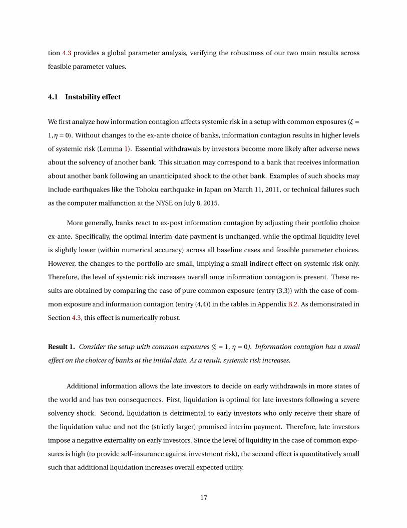
4.1 Instability effect

We first analyze how information contagion affects systemic risk in a setup with common exposures (ξ=1,η= 0). Without changes to the ex-ante choice of banks, information contagion results in higher levels

of systemic risk (Lemma 1). Essential withdrawals by investors become more likely after adverse news

about the solvency of another bank. This situation may correspond to a bank that receives information

about another bank following an unanticipated shock to the other bank. Examples of such shocks may

include earthquakes like the Tohoku earthquake in Japan on March 11, 2011, or technical failures such

as the computer malfunction at the NYSE on July 8, 2015.

More generally, banks react to ex-post information contagion by adjusting their portfolio choice

ex-ante. Specifically, the optimal interim-date payment is unchanged, while the optimal liquidity level

is slightly lower (within numerical accuracy) across all baseline cases and feasible parameter choices.

However, the changes to the portfolio are small, implying a small indirect effect on systemic risk only.

Therefore, the level of systemic risk increases overall once information contagion is present. These re-

sults are obtained by comparing the case of pure common exposure (entry (3,3)) with the case of com-

mon exposure and information contagion (entry (4,4)) in the tables in Appendix B.2. As demonstrated in

Section 4.3, this effect is numerically robust.

Result 1. Consider the setup with common exposures (ξ = 1, η = 0). Information contagion has a small

effect on the choices of banks at the initial date. As a result, systemic risk increases.

Additional information allows the late investors to decide on early withdrawals in more states of

the world and has two consequences. First, liquidation is optimal for late investors following a severe

solvency shock. Second, liquidation is detrimental to early investors who only receive their share of

the liquidation value and not the (strictly larger) promised interim payment. Therefore, late investors

impose a negative externality on early investors. Since the level of liquidity in the case of common expo-

sures is high (to provide self-insurance against investment risk), the second effect is quantitatively small

such that additional liquidation increases overall expected utility.

17

4.2 Resilience effect

We turn to the case of counterparty risk (ξ= 0, η> 0). If the ex-ante choices of banks are unaltered, sys-

temic risk mechanically increases (Lemma 2). This result arises directly from the fact that a failure of the

creditor bank becomes more likely after adverse news about the solvency of the debtor bank. Therefore,

information contagion strengthens the effect of counterparty risk, which leads to a lower level of ex-

pected utility and higher systemic risk. This immediate result is also obtained numerically by comparing

entries in the tables in Appendix B.2, notably entry (1,1) for the case of pure counterparty risk with entry

(1,2) for the case of counterparty risk and information contagion. In this comparison, both are evaluated

at the optimal choices of the pure counterparty risk case (so ex-ante choices are not adjusted).

The focus of this paper is on studying the effect of information contagion on systemic risk, taking

information contagion at the interim date into account. As a result, banks alter their portfolio choices at

the initial date. Specifically, a bank makes a more prudent portfolio choice to insure risk-averse investors

against potential information contagion at the interim date. First, banks reduce the exposure to counter-

party risk by engaging in less liquidity co-insurance (lower b). To cover the liquidity demand from early

investors, a bank increases the amount of storage (larger y), which is akin to liquidity self-insurance.

This reduces the investment in the risky project and funds a larger amount of insurance against idiosyn-

cratic liquidity risk (larger d). The more prudent portfolio choices reduce the range of solvency shocks

([θCI S ,θ

CI F ]) for which counterparty risk after information contagion occurs. These results are obtained

numerically by comparing the case of pure counterparty risk (entry (1,1)) with the case of counterparty

risk and information contagion (entry (2,2)) in the tables in Appendix B.2.

The crucial insight is that the mechanical positive effect of information contagion on systemic risk

(Result 2) is more than fully compensated for by an indirect negative effect via the change in the ex-

ante portfolio choice. Therefore, the overall effect is a reduction in systemic risk because of information

contagion. We label this the resilience effect. In section 4.3, we show that this result holds across all

feasible parameter values.

Result 2. Consider the setup with counterparty risk (ξ= 0, η> 0). Information contagion induces a more

prudent portfolio choice ex ante: liquidity co-insurance, which exposes banks to counterparty risk, is sub-

stituted by direct holdings of liquidity (self-insurance) that reduces the investment in the risky project. The

overall effect is a reduction in both expected utility and systemic risk.

18

4.3 Robustness checks

This section shows that the resilience effect and the instability effect are robust to exogenous parameter

variations. In particular, we discuss a global variation of parameters by considering the entire range of

feasible parameters and study the effect on both systemic risk and expected utility. Details are contained

in the Appendix.

Consider the resilience effect (Result 2) first. Figure 1 displays the expected utility (dotted line)

and systemic risk (dashed line) in the case of counterparty risk and information contagion as a fraction

of their respective levels in the case of pure counterparty risk. The resilience effect is present if relative

systemic risk is below unity. We consider parameter changes of the key variables of the model: the liq-

uidation value (β), the return on investment in the good state (R), the proportion of early investors (λ),

and the level of transparency (q). In all cases, the resilience effect prevails.

There are parameters for which the resilience effect is too small and information contagion does

not reduce systemic risk. Although the resilience effect does not hold for all parameter values, we can

quantify whether or not it holds on average. To test this, we formulate the following hypothesis:

Hypothesis 1. Information contagion due to counterparty risk does not reduce systemic risk.

Since we cannot assume that the difference between SRCR+IC and SRCR is normally distributed, we

test Hypothesis 1 using the Wilcoxon signed rank sum test. The null hypothesis is that SRCR+IC = SRCR.

The results of this analysis show a significant difference in systemic risk in the two cases, z = −116.697,

p < 0.01, indicating that systemic risk in the case of counterparty risk and information contagion is sig-

nificantly lower than in the case of pure counterparty risk.

Turning to the instability effect (Result 1), we see that Figure 2 displays the expected utility (dotted

line) and systemic risk (dashed line) in the case of common exposure and information contagion as a

fraction of their respective levels in the case of pure common exposure. Hence, the instability effect is

present if the relative systemic risk is above unity. We consider the same parameter changes again. In all

cases, the instability effect prevails.

19

5 Conclusion

The aftermath of the failure of Lehman Brothers in September 2008 suggests that information contagion

can be a major source of systemic risk, defined as the probability of joint default of banks. One bank’s

investors will find information about another bank’s solvency valuable for two reasons. First, both banks

may have invested in the same asset class, such as risky sovereign debt or mortgage-backed securities.

Learning about another bank’s profitability will help the investor assess the profitability of its bank. Sec-

ond, one bank may have lent to the other, for instance to share liquidity risk. Knowledge of the debtor

bank’s profitability helps investors assess the counterparty risk of the creditor bank.

We offer a model of systemic risk with information contagion. News about the health of one bank

is valuable for the investors of another bank because of common exposures or counterparty risk. In each

case, bad news about one bank adversely spills over to other banks and causes information contagion.

We study its effects on the bank’s ex-ante choices and the implied level of systemic risk.

We demonstrate that information contagion can reduce systemic risk. When banks are subject to

counterparty risk, investors in one bank may receive a negative signal about the health of another bank.

Given the exposure of the creditor bank to the debtor bank, adverse information about the debtor bank

can cause a run on the creditor bank. Such information contagion ex-post induces the bank to hold

a more prudent portfolio ex-ante. Banks reduce their exposure to counterparty risk and rely more on

self-insurance of liquidity instead of co-insurance. Overall, the level of systemic risk is actually reduced

with information contagion. Moreover, the effects of information contagion on systemic risk depend on

the source of the revealed information. The case of common exposures, ex-post information contagion

increases systemic risk – similar to Acharya and Yorulmazer (2008a).

20

References

Acharya, V. V. and T. Yorulmazer (2008a). Cash-in-the-market pricing and optimal resolution of bank

failures. Review of Financial Studies 21(6), 2705–2742.

Acharya, V. V. and T. Yorulmazer (2008b). Information contagion and bank herding. Journal of Money,

Credit and Banking 40(1), 215–231.

Ahnert, T. (2016). Rollover Risk, Liquidity, and Macroprudential Regulation. Journal of Money, Credit and

Banking, 48(8), 1753–85.

Ahnert, T. and A. Kakhbod (2017). Information choice and amplification of financial crises. Review of

Financial Studies 30(6), 2130–78.

Allen, F., A. Babus, and E. Carletti (2012). Asset commonality, debt maturity and systemic risk. Journal of

Financial Economics 104, 519–534.

Allen, F. and D. Gale (1998). Optimal financial crises. Journal of Finance 53(4), 1245–1284.

Allen, F. and D. Gale (2000). Financial contagion. Journal of Political Economy 108, 1–33.

Allen, F. and D. Gale (2007). Understanding Financial Crises. Oxford University Press.

Brunnermeier, M. (2009). Deciphering the liquidity crunch of 2007/2008. Journal of Economic Perspec-

tives, 77–100.

Carlsson, H. and E. van Damme (1993, September). Global games and equilibrium selection. Economet-

rica 61(5), 989–1018.

Chen, Y. (1999). Banking panics: The role of the first-come, first-served rule and information externali-

ties. Journal of Political Economy 107(5), 946–968.

Cooper, R. and T. W. Ross (1998). Bank runs: Liquidity costs and investment distortions. Journal of

Monetary Economics 41(1), 27–38.

Dasgupta, A. (2004). Financial contagion through capital connections: A model of the origin and spread

of bank panics. Journal of the European Economic Association 2(6), 1049–1084.

Diamond, D. and P. Dybvig (1983). Bank runs, deposit insurance and liquidity. Journal of Political Econ-

omy 91, 401–419.

21

Ennis, H. M. and T. Keister (2006). Bank runs and investment decisions revisited. Journal of Monetary

Economics 53(2), 217–232.

Freixas, X., B. M. Parigi, and J. C. Rochet (2000). Systemic risk, interbank relations, and liquidity provision

by the central bank. Journal of Money, Credit and Banking 32(3), 611–638.

Goldstein, I. and A. Pauzner (2005). Demand deposit contracts and the probability of bank runs. Journal

of Finance 60(3), 1293–1327.

Inada, K.-I. (1963). On a two-sector model of economic growth: Comments and a generalization. Review

of Economic Studies 30(2), 119–127.

Jacklin, C. J. and S. Bhattacharya (1988). Distinguishing panics and information-based bank runs: Wel-

fare and policy implications. Journal of Political Economy 96(3), 568–592.

Leitner, Y. (2005). Financial networks: Contagion, commitment, and private sector bailouts. Journal of

Finance 60, 2925 – 53.

Morris, S. and H. S. Shin (2003). Global games: Theory and applications. Cambridge University Press,

Advances in Economics and Econometrics, the Eighth World Congress.

Nash, J. (1951). Non-cooperative games. Annals of Mathematics 354(2), 286–295.

Postlewaite, A. and X. Vives (1987). Bank runs as an equilibrium phenomenon. Journal of Political Econ-

omy 95, 485 – 491.

Rochet, J.-C. and X. Vives (2004). Coordination failures and the lender of last resort: was bagehot right

after all? Journal of the European Economic Association 2(6), 1116–1147.

The Bank for International Settlements (1997). Financial stability in emerging markets economies.

Draghi Report of the Working Party on Financial Stability in Emerging Market Economies, Bank for

International Settlements.

Vives, X. (2014). Strategic complementarity, fragility, and regulation. Review of Financial Studies 27(12),

3547–3592.

Wagner, W. (2011). Systemic liquidation risk and the diversity-diversification trade-off. Journal of Fi-

nance 66(4), 1141 – 1175.

22

A Figures

0.2

0.4

0.6

0.8

1

1.2

0.3 0.4 0.5 0.6 0.7 0.8 0.9 1

beta

EU[CR+IC]/EU[CR]A[CR+IC]/A[CR]

0.2

0.4

0.6

0.8

1

1.2

0.3 0.4 0.5 0.6 0.7

lambda


0.2

0.4

0.6

0.8

1

1.2

4 6 8 10 12 14 16 18 20

R


0.2

0.4

0.6

0.8

1

1.2

0.1 0.2 0.3 0.4 0.5 0.6 0.7 0.8 0.9qH


Figure 1: Robustness check. The resilience effect (Result 2) obtains for all parameter variations. Weconsider variations of β (top left), R (top right), λ (bottom left), and q (bottom right). The figures displayexpected utility (dotted line) and the level of systemic risk (dashed line) in the case of counterparty riskand information contagion as a fraction of their respective levels in the case of pure counterparty risk.

23

0.8

0.9

1

1.1

1.2

1.3

1.4

1.5

1.6

0.3 0.4 0.5 0.6 0.7 0.8 0.9 1

beta

EU[CE+IC]/EU[CE]A[CE+IC]/A[CE]

0.8

0.9

1

1.1

1.2

1.3

1.4

1.5

1.6

0.3 0.4 0.5 0.6 0.7

lambda

EU[CE+IC]/EU[CR]A[CE+IC]/A[CE]

0.8

0.9

1

1.1

1.2

1.3

1.4

1.5

1.6

4 6 8 10 12 14 16 18 20

R


0.8

0.9

1

1.1

1.2

1.3

1.4

1.5

1.6

0.1 0.2 0.3 0.4 0.5 0.6 0.7 0.8 0.9qH


Figure 2: Robustness check. The instability effect (Result 1) obtains for all parameter variations. Weconsider variations of β (top left), R (top right), λ (bottom left), and q (bottom right). The figures displayexpected utility (dotted line) and the level of systemic risk (dashed line) in the case of common exposuresand information contagion as a fraction of their respective levels in the case of pure common exposures.

24

B Tables

Section B.1 contains the extreme parameter value benchmarks discussed in Section 3.3 of the main text

for additional baseline cases to show the robustness of our numerical implementation. Section B.2 con-

tains the results of Sections 4.1 and 4.2 of the main text. Finally, Section B.3 contains the summary statis-

tics for the parameters used in our global parameter analysis in Section 4.3.

B.1 Extreme parameter value benchmarks

Baseline 1 Baseline 2 Baseline 3 Baseline 4

R = 1.0 y∗ = 0.98 y∗ = 0.98 y∗ = 0.98 y∗ = 0.98ρ = 0.0 d∗

1 = 0.0 d∗1 = 0.0 d∗

1 = 0.0 d∗1 = 0.0

y∗ = 0.0 y∗ = 0.0 y∗ = 0.0 y∗ = 0.0ρ = 200.0 d∗

1 = 0.98 d∗1 = 0.98 d∗

1 = 0.98 d∗1 = 0.98

y∗ = 0.98 y∗ = 0.98 y∗ = 0.98 y∗ = 0.98η= 0.0 b∗ = 0.0 b∗ = 0.0 b∗ = 0.0 b∗ = 0.0ϕ= 0.0 b∗ = 0.15 b∗ = 0.15 b∗ = 0.15 b∗ = 0.1λ= 0.01 d∗

1 = 1.06 d∗1 = 1.0 d∗

1 = 1.1 d∗1 = 1.16

y∗ = 0.42 y∗ = 0.36 y∗ = 0.48 y∗ = 0.74λ= 0.99 d∗

1 = 0.98 d∗1 = 0.98 d∗

1 = 0.98 d∗1 = 0.98

y∗ = 0.98 y∗ = 0.98 y∗ = 0.98 y∗ = 0.98q.0 A1, . . . , A6 = 0.0 A1, . . . , A6 = 0.0 A1, . . . , A6 = 0.0 A1, . . . , A6 = 0.0

Table 2: Extreme parameter values for four baseline cases. Baseline 1: β = 0.7, R = 5.0 ϕ = 1.0, λ = 0.5,η = 0.25, ρ = 1.0, q = 0.7. Baseline 2: β = 0.7, R = 5.0 ϕ = 1.0, λ = 0.5, η = 0.25, ρ = 0.9, q = 0.7. Baseline3: β = 0.7, R = 5.0 ϕ = 1.0, λ = 0.5, η = 0.25, ρ = 1.1, q = 0.7. Baseline 4: β = 0.3, R = 5.0 ϕ = 1.0, λ = 0.5,η= 0.25, ρ = 1.1, q = 0.7.

25

B.2 Results

cr cr + ic ce ce + ic(EU , d∗

1 , y∗, b∗) (EU , d∗1 , y∗, b∗) (EU , d∗

1 , y∗, b∗) (EU , d∗1 , y∗, b∗)

(θD

, θCNI , Acr) (θ

D, θ

CI S , θ

CI F , Acr+ic) (θ, Ace) (θ, Ace+ic)

cr (0.172,0.88,0.73,0.08) (0.096,0.88,0.73,0.08)(0.423,0.23,0.048) (0.423,0.212,0.252,0.052)

cr + (0.107,0.94,0.8,0.02)ic (0.379,0.211,0.222,0.041)

ce (0.13,1.0,0.77,0.0) (0.137,1.0,0.77,0.0)(0.328,0.161) (0.328,0.161)

ce + (0.137,1.01,0.76,0.0)ic (0.344,0.168)

Table 3: Equilibrium allocation for different forms of financial fragility for calibrationβ=0.7, R=5.0, ϕ=1.0,λ=0.5, η=0.25, ρ=1.0, qH =0.7. Expected utility (EU ), portfolio choice variables (d1, y,b), withdrawal

thresholds (θH ,θ1,L ,θN2,L ,θ

D2,L ,θ), and systemic financial fragility (Acr, Acr+ic, Ace, Ace+ic) in the different

model variants (cr: counterparty risk, ic: information contagion, ce: common exposure).


1 , y∗, b∗) (EU , d∗1 , y∗, b∗) (EU , d∗

1 , y∗, b∗) (EU , d∗1 , y∗, b∗)

(θD

, θCNI , Acr) (θ

D, θ

CI S , θ


cr (0.188,0.86,0.7,0.13) (0.105,0.86,0.7,0.13)(0.482,0.304,0.072) (0.482,0.278,0.329,0.078)

cr + (0.117,0.93,0.78,0.06)ic (0.43,0.26,0.283,0.06)

ce (0.142,1.0,0.75,0.0) (0.154,1.0,0.75,0.0)(0.373,0.183) (0.373,0.183)

ce + (0.158,1.32,0.73,0.0)ic (0.5,0.245)





26


1 , y∗, b∗) (EU , d∗1 , y∗, b∗) (EU , d∗

1 , y∗, b∗) (EU , d∗1 , y∗, b∗)

(θD

, θCNI , Acr) (θ

D, θ

CI S , θ


cr (0.343,0.84,0.69,0.14) (0.221,0.84,0.69,0.14)(0.372,0.172,0.031) (0.372,0.15,0.206,0.038)

cr + (0.238,0.91,0.77,0.07)ic (0.318,0.139,0.166,0.026)

ce (0.274,1.0,0.75,0.0) (0.28,1.0,0.75,0.0)(0.257,0.126) (0.257,0.126)

ce + (0.28,1.01,0.74,0.0)ic (0.271,0.133)

Table 5: Equilibrium allocation for different forms of financial fragility for calibration β=0.7, R=10.0,ϕ=1.0, λ=0.5, η=0.25, ρ=1.0, qH =0.7. Expected utility (EU ), portfolio choice variables (d1, y,b), with-

drawal thresholds (θH ,θ1,L ,θN2,L ,θ

D2,L ,θ), and systemic financial fragility (Acr, Acr+ic, Ace, Ace+ic) in the dif-

ferent model variants (cr: counterparty risk, ic: information contagion, ce: common exposure).


1 , y∗, b∗) (EU , d∗1 , y∗, b∗) (EU , d∗

1 , y∗, b∗) (EU , d∗1 , y∗, b∗)

(θD

, θCNI , Acr) (θ

D, θ

CI S , θ


cr (0.262,0.83,0.6,0.07) (0.151,0.83,0.6,0.07)(0.404,0.258,0.051) (0.404,0.249,0.271,0.054)

cr + (0.166,0.92,0.7,0.01)ic (0.35,0.231,0.234,0.04)

ce (0.182,1.01,0.68,0.0) (0.192,1.01,0.68,0.0)(0.313,0.153) (0.313,0.153)

ce + (0.192,1.02,0.66,0.0)ic (0.327,0.16)





27


1 , y∗, b∗) (EU , d∗1 , y∗, b∗) (EU , d∗

1 , y∗, b∗) (EU , d∗1 , y∗, b∗)

(θD

, θCNI , Acr) (θ

D, θ

CI S , θ


cr (0.232,0.82,0.69,0.0) (0.071,0.82,0.69,0.0)(0.36,0.236,0.014) (0.36,0.236,0.236,0.014)

cr + (0.099,0.94,0.82,0.0)ic (0.331,0.207,0.207,0.011)

ce (0.121,1.0,0.79,0.0) (0.128,1.0,0.79,0.0)(0.313,0.05) (0.313,0.05)

ce + (0.128,1.0,0.78,0.0)ic (0.321,0.051)





28

B.3 Global Parameter Analysis

This section presents details for the N = 640,000 simulation runs we conducted in Section 4.3 to test

whether the resilience effect will hold in the entire parameter space, at least on average.

Table 8: Summary Statistics for Model Parameters.

Variable N mean sd min p25 median p75 max

R 640,000 5.499 2.599 1.000 3.248 5.498 7.748 10.000β 640,000 0.500 0.283 0.010 0.255 0.500 0.745 0.990λ 640,000 0.500 0.144 0.250 0.375 0.499 0.625 0.750η 640,000 0.125 0.066 0.010 0.067 0.125 0.182 0.240ϕ 640,000 1.000 0.115 0.800 0.900 1.000 1.100 1.200q 640,000 0.500 0.289 0.000 0.250 0.499 0.751 1.000ρ 640,000 1.750 0.433 1.000 1.374 1.749 2.125 2.500

Note: Each parameter is drawn independently of the others from a uniform distribution. R is the positive realization of thereturn of the risky asset, β the liquidation value, λ the probability of being an early investor, η the size of the liquidity shock,ϕ the price of co-insurance, q the investors’ probability of being informed about the solvency shock in the other region, andρ the risk-aversion parameter for the constant relative risk aversion utility used. sd, p25, and p75 are the standard deviationand the 25th and 75th percentiles of the observable distribution, respectively.

29

Table 9: Summary Statistics for Observables in the Case With Counterparty Risk.

Variable N mean sd min p25 median p75 max

Expected Utility [cr] 640,000 -8.361 495.169 -329720.656 -2.579 -1.267 -0.834 -0.528Systemic Risk [cr] 640,000 0.043 0.058 0.000 0.000 0.017 0.060 0.250Payoff to Early Investors [cr] 640,000 1.042 0.056 0.856 1.010 1.024 1.066 1.486Self-Insurance [cr] 640,000 0.899 0.064 0.500 0.860 0.910 0.940 0.990Co-Insurance [cr] 640,000 0.103 0.079 0.000 0.041 0.091 0.151 0.360

Expected Utility [cr+ic] 640,000 -2.2·1014 1.4·1015 -1.0·1016 -2.800 -1.309 -0.848 -0.528Systemic Risk [cr+ic] 640,000 0.043 0.058 0.000 0.004 0.017 0.053 0.250Payoff to Early Investors [cr+ic] 640,000 1.027 0.051 0.884 0.996 1.010 1.038 1.486Self-Insurance [cr+ic] 640,000 0.907 0.061 0.500 0.870 0.910 0.950 0.990Co-Insurance [cr+ic] 640,000 0.019 0.034 0.000 0.000 0.000 0.032 0.359

Expected Utility [ce] 640,000.000 -8.365 495.169 -329720.6 -2.582 -1.271 -0.837 -0.543Systemic Risk [ce] 640,000.000 0.118 0.128 0.000 0.018 0.073 0.171 0.500Payoff to Early Investors [ce] 640,000.000 1.053 0.080 0.954 1.010 1.024 1.052 1.486Self-Insurance [ce] 640,000.000 0.902 0.063 0.400 0.870 0.910 0.940 0.990

Expected Utility [ce+ic] 640,000.000 -8.360 495.169 -329720.6 -2.578 -1.266 -0.833 -0.528Systemic Risk [ce+ic] 640,000.000 0.247 0.158 0.000 0.120 0.209 0.414 0.500Payoff to Early Investors [ce+ic] 640,000.000 1.100 0.134 0.940 1.010 1.038 1.136 1.486Self-Insurance [ce+ic] 640,000.000 0.893 0.072 0.370 0.860 0.900 0.940 0.990

Expected Utility [cr+ic (non-optimal)] 640,000 -2.0·1013 4.5·1014 -1.0·1016 -2.609 -1.281 -0.844 -0.528Systemic Risk [cr+ic (non-optimal)] 640,000 0.051 0.060 0.000 0.004 0.029 0.075 0.250

Expected Utility [ce+ic (non-optimal)] 640,000.000 -8.365 495.169 -329720.6 -2.582 -1.271 -0.837 -0.543Systemic Risk [ce+ic (non-optimal)] 640,000.000 0.226 0.141 0.000 0.119 0.204 0.305 0.500

Note: Expected Utility and Systemic Risk (defined as the joint default probability of the two banks) are measured ex-ante.Payoff to Early Investors, Self-Insurance, and Co-Insurance are ex-ante optimal payoffs promised to impatient investors, d1,the amount of self-insurance y , and the amount of co-insurance b, respectively. [cr] denotes the pure counterparty risk case,[cr+ic] the case of counterparty risk and information contagion, both evaluated at their ex-ante optimal portfolio choices.[cr+ic (non-optimal)] is the case of counterparty risk and information contagion evaluated at the optimal portfolio choiceof the pure counterparty risk case; sd, p25, and p75 are the standard deviation and the 25th and 75th percentile of theobservable distribution, respectively.

30

information contagion and systemic risk - bank of …...2 bank of canada staff working paper 2017-29...

Documents