systemic risk : channels of contagion in financial systems...

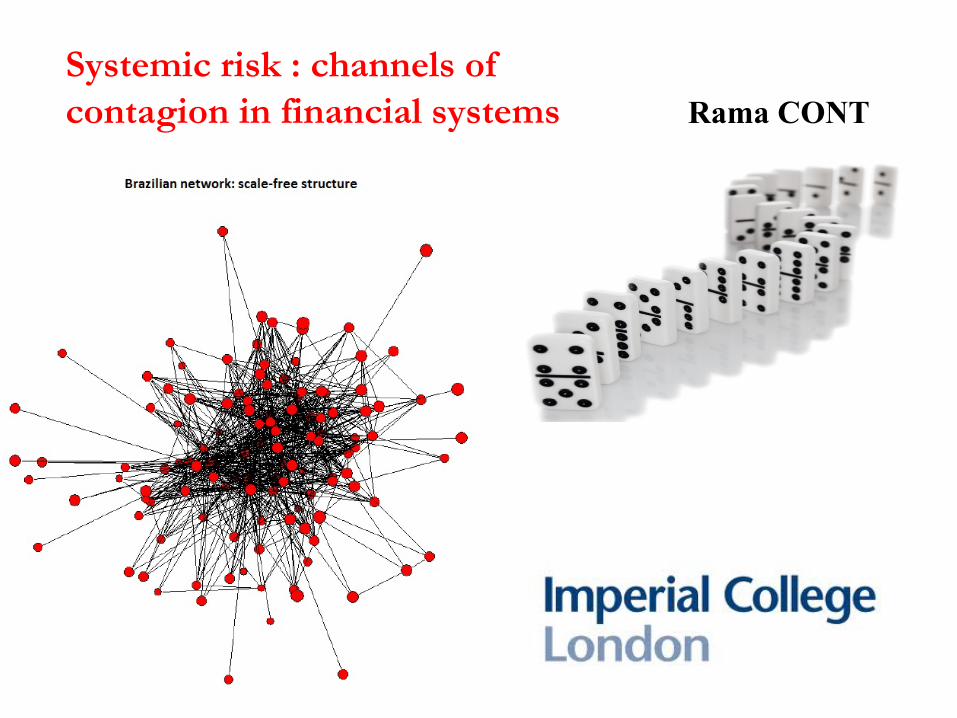
Systemic risk : channels of contagion in financial systems Rama CONT

Rama CONT: Contagion and systemic risk in financial networks

Systemic Risk •  Systemic risk may be defined as the risk that a significant

portion of the financial system fails to function properly. •  The monitoring and management of systemic risk has become

a major issue for regulators and market participants since the 2008 crisis.

•  The financial crisis has simultaneously underlined · the importance of contagion effects and systemic risk · the lack of adequate indicators for monitoring systemic risk. · the lack of adequate data for computing such indicators Many initiatives under way: new regulations (Basel III), new

financial architecture (derivatives clearinghouses), legislation on transparency in OTC markets, creation of Office of Financial Research (US), various Financial Stability Boards

BUT: methodological shortcomings, open questions


Systemic Risk Various questions: Mechanisms which lead to systemic risk Measures / metrics of systemic risk Monitoring of systemic risk: data type/granularity ? Management and control of systemic risk by regulators Need for quantitative approaches and objective criteria

to deal with these questions


Channels of contagion: underlying network structure

•  Each of these mechanism may be viewed as a contagion process on some underlying “network”, but the relevant “network topologies’’ and data needed to track them are different in each case:

•  1. Correlation: cross-sectional data on common exposures to risk factors/asset classes for tracking large-scale imbalances

•  2. Balance sheet contagion: network of interbank exposures, cross-holdings and liabilities + capital

•  3. Spirals of illiquidity: network of short-term liabilities (payables) and receivables + ‘liquidity reserves’

•  4. Fire sales/ feedback effects: data on portfolio holdings of financial institutions across asset classes + capital

!  R Cont, A Moussa, E B Santos (2013)Network structure and systemic risk in banking systems in: Handbook of Systemic Risk, Cambridge Univ Press.

!  H Amini, R Cont, A Minca (2012) Stress testing the resilience of financial networks, Intl Journal of Theoretical and applied finance, Vol 15, No 1.

!  H Amini, R Cont, A Minca (2011)Resilience to contagion in financial networks, to appear in Mathematical Finance.

!  R Cont & L Wagalath (2013) Running for the exit: distressed selling and endogenous correlation in financial markets, Mathematical Finance, Vol 23 (4), 718-741.

!  R Cont & Th Kokholm (2014) Central clearing of OTC derivatives: bilateral vs multilateral netting, Statistics and Risk Modeling, Vol 31, 1, 3-22.

!  R Cont & L Wagalath (2012) Fire sales forensics: measuring endogenous risk, to appear in Mathematical Finance.

!  R Cont & E Schaanning (2014) Fire sales, endogenous risk and price-mediated contagion:

modeling, monitoring and prudential policy, Isaac Newton Institute Working Paper.

Lecture 1: Contagion and systemic risk infinancial networks

Rama Cont

Imperial College London&

Centre National de Recherche Scientifique (CNRS), Paris

[email protected]

Joint work with:Hamed Amini (EPFL) Amal Moussa (Columbia)

Andreea Minca (Cornell) Lakshithe Wagalath (Paris VI)

Rama Cont Network models of contagion and systemic risk

A"bank"balance"sheet"

Assets" Liabili/es"

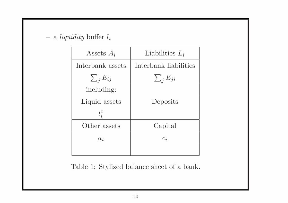
– a liquidity buffer !!

Assets "! Liabilities #!

Interbank assets Interbank liabilities∑

" $!"∑

" $"!

including:

Liquid assets Deposits

!0!

Other assets Capital

%! &!

Table 1: Stylized balance sheet of a bank.

10

Insolvency and illiquidity •  Equity + Debt= Total assets. •  Capital= Equity is not to be confused with cash/liquid reserves. •  If Total assets < Debt then firm is insolvent. •  If “liquid assets” < payables, firm is illiquid. •  Liquidity reserves vary rapidly (intraday) while asset and debt values are more “slowly varying”. •  Default occurs when firm fails to meet payables (margin call, coupon, interest on debt). This is a

liquidity issue. •  A firm can become illiquid even though it is perfectly sovlent. But in principle such a firm will not

default: it can borrow against its assets. •  In principle, insolvency does not immediately entail default as long as payments due are met. •  However, when the firm is a bank/ financial institution: -the regulator monitors capital and may liquidate/restructure bank as insolvency threshold is reached -most financial institutions hold a very small reserve of liquid assets and cover their short term liquidity needs through short term (overnight) loans. In this situation insolvency (or, indeed, a rumour of insolvency) leads to lenders withdrawing the firms funding and lead to illiquidity Lender of last resort: if a bank is solvent but temporarily illiquid, the central bank can provide liquidity (lend) to it until liquidity is restored. Bagehot’s principle: lend to solvent banks, but at a penalty. These considerations justify to focus the modeling of bank failure and contagion on insolvency which is the fundamental notion of failure for a bank.


The ‘microprudential’ approach to financial stability Traditional approach to risk management and bank regulation:

focused on failure/non-failure (solvency, liquidity) of individual banks

Focuses on balance sheet structure of individual banks Risk of each bank’s portfolio is measured using a statistical

approach based on historical data: assumes that losses arises due to exogenous random fluctuations in risk factors (stock prices, exchange rates, interest rates, housing prices..)

Main tool for stabilization of system: capital requirements Based on premise that ‘it is enough to supervise the stability of

each bank to ensure stability of system’ Ignores links or interactions between market participants which

can lead to market instabilities even when banks are ‘well capitalized’ (Hellwig 1995, 1998; Rochet & Tirole 1996; Freixas, Parigi & Rochet 2000)


Why systemic risk does not reduce to ‘marginal risk’ Example 1 (Hellwig): liability chains Consider a finite set of banks i=1..N, where

i borrows $ 100 from i-1over i years, i lends $ 100 to i+1 over i+1 years, etc.

Each institution in this “lending chain” is exposed to ‘market risk’ due to the difference (spread) between the i-year interest rate r(i) and the i+1 year interest rate r(i+1).

Net exposure of i= X(i)=100 ( r(i+1)-r(i) ) A microprudential approach asks for capital requirements based on a quantile

of X(i) or some other tail measure: Typically interest rate volatility is small (few %) so setting a capital

requirement of a few % covers this marginal risk. However, if bank i fails (defaults), then counterparty i-1 is left completely

exposed: exposure in case of default is E(i)=100 >> X(i)

1998: “Long Term Capital Management”

∙ Size= 4 billion$, Daily VaR= 400 million $ in Aug 1998.

∙ Amaranth (2001): size = 9.5 billion USD, no systemic

consequence.

∙ The default of Amaranth hardly made headlines: no systemic

impact.

∙ The default of LTCM threatened the stability of the US

banking system → Fed intervention

∙ Reason: LTCM had many counterparties in the world banking

system, with large liabilities/exposures.

∙ 1: Systemic impact is not about ’net’ size but related to

exposures/ connections with other institutions.

∙ 2: a firm can have a small magnitude of losses/gains AND be a

source of large systemic risk

4


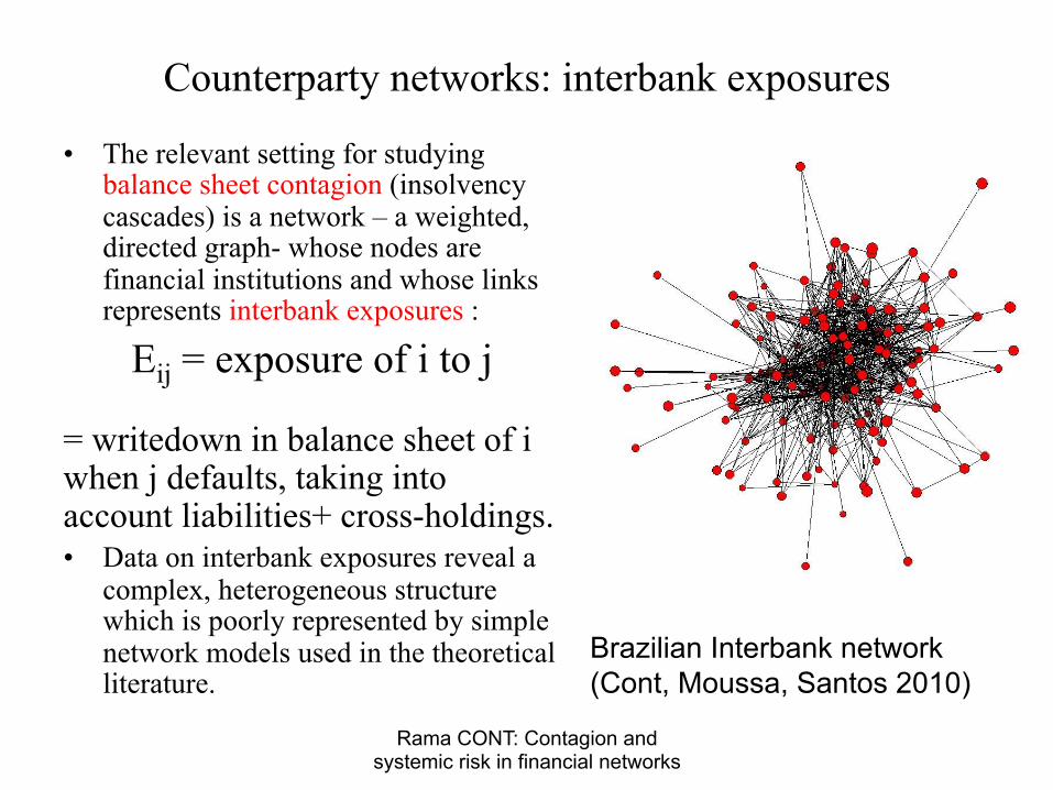
Counterparty networks: interbank exposures

•  The relevant setting for studying balance sheet contagion (insolvency cascades) is a network – a weighted, directed graph- whose nodes are financial institutions and whose links represents interbank exposures :

Eij = exposure of i to j = writedown in balance sheet of i when j defaults, taking into account liabilities+ cross-holdings. •  Data on interbank exposures reveal a

complex, heterogeneous structure which is poorly represented by simple network models used in the theoretical literature.

Brazilian Interbank network (Cont, Moussa, Santos 2010)

Measuring systemic risk: why exposures areimportant inputs

Market-based indicators have been recently proposed for

quantifying

∙ contagion effects: CoVaR (quantile regression of past bank

portfolio losses, Adrian & Brunnenmeier 2009)

∙ the (global) level of systemic risk in the financial system (Lehar

2005, Bodie, Gray, Merton 2008, IMF 2009, Huang, Zhu &

Zhou 2010, Acharya et al 2010,..)

Useful for analyzing past/current economic data and should be

part of any risk dashboard/ systemic risk tool kit.

Value as forward-looking diagnosis tools? any predictive ability?

18

Also: market-implied measures capture market-perceived systemic

risk. Did market prices capture the systemic risk of AIG prior to

its collapse?

Network approaches are based on exposures which represent

potential future losses, which can give quite a different picture

from past losses.

Even if we believe the Efficient Market hypothesis, market

indicators need not reflect exposures, which are not public

information.

Regulators, on the other hand, have access to non-public

information on exposures and should use such information for

stress testing and for computing systemic risk indicators.

19

Regulatory reforms proposed for mitigating systemic risk include

1 monitoring and control of nodes (balance sheets):higher capital ratios: increasing resilience of nodes to potential lossesLiquidity Coverage Ratio, Stable Funding Ratio: to prevent defaultcontagion through loss of short term liabilitiesother: leverage ratio,

2 monitoring and control of links : proposals for structural reformCentral clearing of OTC derivatives: introduce a new node (CentralCounterparty) and replace bilateral OTC exposures by exposures toCCPRing-fencing (Vickers, Liikanen): separatd the network into a tightlyregulated core of retail banks and a less regulated set of otherinstitutions, with strict limits on links between these twosubnetworks.

Underlying these proposals is the question of the relation betweennetwork structure on one hand and the resilience of the network to

shocks on the other hand.


Figure: Network structures of real-world banking systems. Austria:scale-free structure (Boss et al2004), Switzerland: sparse and centralizedstructure (Müller 2006).

Figure: Network structures of real-world banking systems. Hungary:multiple money center structure (Lubloy et al 2006) Brazil: scale-freestructure (Cont, Bastos, Moussa 2010).

The Brazil financial system: a directed scale-free network

∙ Exposures are reportted daily to Brazilian central bank.

∙ Data set of all consolidated interbank exposures (incl. swaps)+

Tier I and Tier II capital (2007-08).

∙ ! ≃ 100 holdings/conglomerates, ≃ 1000 counterparty relations

∙ Average number of counterparties (degree)= 7

∙ Heterogeneity of connectivity: in-degree (number of debtors)

and out-degree (number of creditors) have heavy tailed

distributions

1

!#{", indeg(") = $} ∼ %

$!!"

1

!#{", outdeg(") = $} ∼ %

$!#$%

with exponents &"#, &$%& between 2 and 3.

∙ Heterogeneity of exposures: heavy tailed Pareto distribution

with exponent between 2 and 3.

14

100 101 10210−3

10−2

10−1

100

In Degree

Pr(K

! k

)

" = 2.1997kmin = 6p−value = 0.0847

Network in June 2007

100 101 10210−3

10−2

10−1

100

In Degree

Pr(K

! k

)

" = 2.7068kmin = 13p−value = 0.2354

Network in December 2007

100 101 10210−3

10−2

10−1

100

In Degree

Pr(K

! k

)

" = 2.2059kmin = 7p−value = 0.0858

Network in March 2008

100 101 10210−3

10−2

10−1

100

In Degree

Pr(K

! k

)

" = 3.3611kmin = 21p−value = 0.7911


100 101 10210−3

10−2

10−1

100

In Degree

Pr(K

! k

)

" = 2.161kmin = 6p−value = 0.0134

Network in September 2008

100 101 10210−3

10−2

10−1

100

In Degree

Pr(K

! k

)

" = 2.132kmin = 5p−value = 0.0582

Network in November 2008

Figure 3: Brazilian financial network: distribution of in-degree.

16

0 0.2 0.4 0.6 0.8 10

0.1

0.2

0.3

0.4

0.5

0.6

0.7

0.8

0.9

1

p−value = 0.99998

p−value = 0.99919

p−value = 0.99998

p−value = 0.9182

p−value = 0.9182

Q−Q Plot of In Degree

Pr(K(i)! k)

Pr(K

(j)!

k)

0 0.2 0.4 0.6 0.8 10

0.1

0.2

0.3

0.4

0.5

0.6

0.7

0.8

0.9

1

p−value = 0.99234

p−value = 0.99998

p−value = 0.99998

p−value = 0.99234

p−value = 0.84221

Q−Q Plot of Out Degree

Pr(K(i)! k)

Pr(K

(j)!

k)

0 0.2 0.4 0.6 0.8 10

0.1

0.2

0.3

0.4

0.5

0.6

0.7

0.8

0.9

1

p−value = 0.99998

p−value = 0.9683

p−value = 0.9683

p−value = 0.99234

p−value = 0.64508

Q−Q Plot of Degree

Pr(K(i)! k)

Pr(K

(j)!

k)

Jun/07 vs. Dec/07Dec/07 vs. Mar/08Mar/08 vs. Jun/08Jun/08 vs. Sep/08Sep/08 vs. Nov/0845o line − (i) vs. (j)



Figure 4: Brazilian financial network: stability of degree distribu-

tions across dates.

17

10−9 10−7 10−5 10−3 10−1 10110−4

10−3

10−2

10−1

100

Exposures ! 10−10 in BRL

Pr(X

" x

)

# = 1.9792xmin = 0.0039544p−value = 0.026


10−9 10−7 10−5 10−3 10−110−4

10−3

10−2

10−1

100


Pr(X

" x

)

# = 2.2297xmin = 0.0074042p−value = 0.6

Network in December 2007

10−9 10−7 10−5 10−3 10−110−4

10−3

10−2

10−1

100


Pr(X

" x

)

# = 2.2383xmin = 0.008p−value = 0.214

Network in March 2008

10−10 10−8 10−6 10−4 10−2 10010−4

10−3

10−2

10−1

100


Pr(X

" x

)

# = 2.3778xmin = 0.010173p−value = 0.692


10−10 10−8 10−6 10−4 10−2 10010−4

10−3

10−2

10−1

100


Pr(X

" x

)

# = 2.2766xmin = 0.0093382p−value = 0.384

Network in September 2008

10−9 10−7 10−5 10−3 10−1 10110−3

10−2

10−1

100


Pr(X

" x

)

# = 2.5277xmin = 0.033675p−value = 0.982

Network in November 2008

Figure 6: Brazilian network: distribution of exposures in BRL.

19

Clustering coefficients

Clustering coefficient of a node=

Number of links among neighbors/ Number of possible links among

neighbors

The ratio is between 0 and 1.

For a complete graph, or for a node immersed in a complete

subgraph, the ratio is 1.

For a d-dimensional lattice, clustering → 0 as ! increases.

Small world graphs are characterized by small diameter,

bounded degree and clustering coefficients bounded away from zero.

15

0 0.2 0.4 0.6 0.8 10

0.1

0.2

0.3

0.4

0.5

0.6

0.7

0.8

0.9

1

Clustering coefficient

Distribution of the clustering coefficient

Figure 5: Brazilian network: distribution of clustering coefficient

16

0 20 40 60 80 1000

0.1

0.2

0.3

0.4

0.5June 2007

Degree

Loca

l Clu

ster

ing

Coe

ffici

ent

0 20 40 60 80 1000

0.1

0.2

0.3

0.4

0.5December 2007

Degree

Loca

l Clu

ster

ing

Coe

ffici

ent

0 20 40 60 800

0.1

0.2

0.3

0.4

0.5March 2008

Degree

Loca

l Clu

ster

ing

Coe

ffici

ent

0 20 40 60 80 1000

0.1

0.2

0.3

0.4

0.5June 2008

Degree

Loca

l Clu

ster

ing

Coe

ffici

ent

0 20 40 60 80 1000

0.1

0.2

0.3

0.4

0.5September 2008

Degree

Loca

l Clu

ster

ing

Coe

ffici

ent

0 20 40 60 80 100 1200

0.1

0.2

0.3

0.4

0.5November 2008

Degree

Loca

l Clu

ster

ing

Coe

ffici

ent

Figure 6: Brazilian financial network: degree vs clustering coeffi-

cient. Arbitrarily small clustering coefficients rule out a small world

network.

17

Network models: irrelevant vs irrelevant issues •  Data on interbank exposures reveal a complex, heterogeneous

structure which is poorly represented by simple network models used in the theoretical literature.

•  Key observation is HETEROGENEITY of nodes and exposures, which should warn against the use of simple, homogeneous networks as models for theoretical analysis.

•  There has also been a recent outpour of studies on exposure data using the ‘network’ approach, computing graph-theoretic measures of centrality, PageRank, clustering for interbank networks.

•  It is not clear why these measures have any relation with ‘systemic risk’

•  More precisely, any measure (such as centrality, PageRank,..) which does not use levels of capital as input is, by definition, insensitive to capital requirements and cannot be used in a meaningful analysis of systemic risk

Some Questions

•  How does the default of a bank affect its counterparties, counterparties of counterparties,… (domino effect)?

•  Which are the banks whose defaults generates the largest systemic loss? : identification of SIFIs

•  Can the default of one or few institutions generate a macro-cascade / large-scale instabiity of network?

•  How do the answers to the above depend on network structure? Which features of network structure determine its stability/ resilience to contagion?

Previous work: many simulation studies+ analytical results for average cascade size on homogeneous networks (Watts (2002), Gai & Kapadia (2011),…) Here: analytical results on resilience and cascade size (not just average) for general, heterogeneous networks

Equilibrium analysis: ’clearing vectors’

Consider a situation where all portfolios are simultaneously liquidated anddebtholders are paid o↵ completely if possible and if not, proportionallyto fraction of debt held. Then, any node unable to pay its liabilities uponliquidation will be declared in default.(Eisenberg & Noe 2001): Given a matrix of exposures E and capitalallocations c , a clearing vector is a vector of cash flows p verifying

limited liability: payments made by a node do not exceed the cashflow available to the node;

the priority of debt claims: node receives no value until the node isable to completely pay o↵ all of its outstanding liabilities

proportionality: if default occurs, all liability holders are paid by thedefaulting node in proportion to the size of their nominal claim onfirm assets.

Recovery rate of each firm at ’equilibrium’ is endogenous: it is the ratioof recovered assets to liabilities.(Eisenberg & Noe 2001): A clearing vector always exists: it may becomputed as a fixed point of an iterative ”liquidation process”.


Equilibrium analysis: ’clearing vectors’

Model motivated by the overnight clearing of interbank payment systems:liabilities are realized as cash flows every day.Less realistic as a model for bank default or contagion of large banklosses: in reality

only defaulted firms are liquidated, not all firms.

in absence of default, there is no liquidation: model cannot deal withlarge losses, only true defaults.

liquidation is a lengthy process and, even if eventually a highrecovery rate is realized after liquidation ends, defaulted assets arenot available/liquid immediately after default.

many losses leading to insolvency are not realized as cash flows butmay be pure ’accounting losses’ / writedowns in asset value:immediately after default, these writedowns may be very large,corresponding to very low, or zero (if assets are frozen duringliquidation), ’short term’ recovery rates.

Ex: Lehman default eventually led to 84% recovery rate but took 6months, during which dozens of hedge funds exposed to Lehmandefaulted!


Cascade models

Another approach is to consider the impact on the network of anexogenous shock: this shock can be

the default of a node or set of nodes or, more generally

a loss in asset value across nodes, which may result in a ’downgrade’/ loss in creditworthiness of some nodes

In both situations, counterparties of the node subject to the shockwill be a↵ected through writedowns in asset value, so loss istransmitted through the network.

If the loss transmitted is large relative to the receiving node’s capitalbu↵er, new credit events may occur, resulting in a cascade of

losses.

Such threshold models of cascade processes were first studied in thecontext of social networks (Granovetter 1978; Watts 2002) inhomogeneous networks with identical node characteristics.


Loss Cascades in a counterparty network

Definition (Loss cascade)

Consider an initial configuration with capital levels (c(j), j 2 V ). Wedefine the sequence (ck(j), j 2 V )k�0

as

c

0

(j) = c(j) and ck+1

(j) = max(c0

(j)�X

{i,ck (i)=0}

Eji , 0), (1)

where Ri is the ”recovery rate” for liabilities of institution i after thecredit event. (cn�1

(j), j 2 V ), where n = |V | is the number of nodes inthe network, then represents the remaining capital once all counterpartylosses have been accounted for. The set of insolvent institutions is thengiven by

D(c ,E ) = {j 2 V : cn�1

(j) = 0} (2)

With n nodes, the cascade terminates at most after n � 1 steps.


Example

a(5) b(5) c(5)

d(10) e(25)

f (10) g(10)

7 8

59

75

10

68

9

11

a

Example

a(5) b(5) c(5)

d(10) e(25)

f (10) g(10)

7 8

59

75

10

68

9

11

d(5)

a b

Example

a(5) b(5) c(5)

d(10) e(25)

f (10) g(10)

7 8

59

75

10

68

9

11

d(5) e(18)

a b c

d

Example

a(5) b(5) c(5)

d(10) e(25)

f (10) g(10)

7 8

59

75

10

68

9

11

d(5) e(18)e(3)

f (4)

a b c

d

Example

Contagion lasts 3 rounds.Fundamental defaults: fi j c0(i) = 0g = fag:Contagious defaults: fi j c0(i) > 0 & cT(i) = 0g = fb; c; dg:Total number of defaults: = 4.

a(5) b(5) c(5)

d(10) e(25)

f (10) g(10)

7 8

59

75

10

68

9

11

d(5) e(18)e(3)

f (4)

a b c

d

Default impact

Definition (Default Impact)

The Default Impact DI (i , c ,E ) of a financial institution i 2 V is definedas the total loss in capital in the cascade triggered by the default of i :

DI (i , c ,E ) =X

j2V

c

0

(j)� cfinal(j), (3)

where (cfinal(j), j 2 V )k�0

is the final level of capital at the end of thecascade with initial condition c

0

(j) = c(j) for j 6= i and c

0

(i) = 0.

Default Impact does not include the loss of the institution triggering thecascade, but focuses on the loss this initial default inflicts to the rest ofthe network: it thus measures the loss due to contagion.

Rama Cont Measuring systemic risk

Variants

If one adopts the point of view of deposit insurance, then the relevantmeasure is the sum of deposits across defaulted institutions:

DI (i , c ,E ) =X

j2D(c,E)

Deposits(j).

Alternatively one can focus on lending institutions (e.g. commercialbanks), whose failure can disrupt the real economy. Defining a set C ofsuch core institutions we can compute

DI (i , c ,E ) =X

j2Cc

0

(j)� cfinal(j)


Contagion effects: too rapidly dismissed?

The small magnitude of such “domino” effects has been cited as

justification for ignoring contagion (Furfine 2003, Geneva Report

2008).

Such simulations ignore the impact of correlated market shocks on

bank balance sheets and, therefore, the compounding effect of

market shocks and contagion.

Many studies on domino effects are not based on actual exposures

but either look at a subset of exposures (e.g. FedWire) or

estimate/reconstruct exposures from balance sheet data using

maximum entropy methods (Boss et el, Elsinger et al) which result

in distributing exposures as uniformly as possible across

counterparties. This method can lead to underestimation of

contagion effects.

23

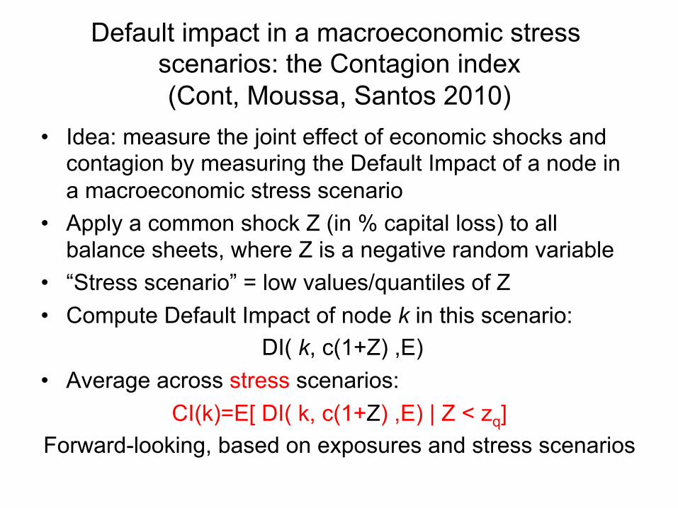
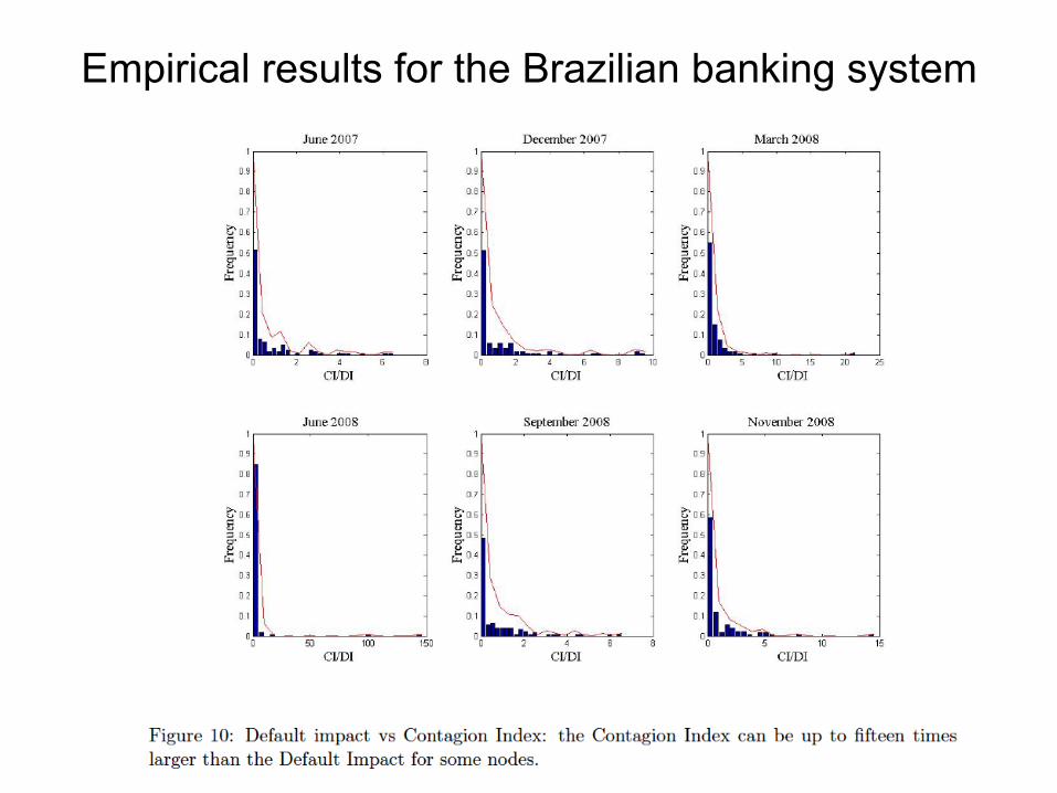
Default impact in a macroeconomic stress scenarios: the Contagion index (Cont, Moussa, Santos 2010)

•  Idea: measure the joint effect of economic shocks and contagion by measuring the Default Impact of a node in a macroeconomic stress scenario

•  Apply a common shock Z (in % capital loss) to all balance sheets, where Z is a negative random variable

•  “Stress scenario” = low values/quantiles of Z •  Compute Default Impact of node k in this scenario:

DI( k, c(1+Z) ,E) •  Average across stress scenarios:

CI(k)=E[ DI( k, c(1+Z) ,E) | Z < zq] Forward-looking, based on exposures and stress scenarios

Heterogeneous stress scenarios

Macroeconomic shocks a↵ect bank portfolios in a highly correlated way,due to common exposures of these portfolios.Moreover, in market stress scenarios fire sales may actually exacerbatesuch correlations.In many stress-testing exercises conducted by regulators, the shocksapplied to various portfolios are actually scaled version of the samerandom variable i.e. perfectly correlated across portfolios.A generalization is to consider co-monotonic shocks generated by acommon factor Z :

✏(i ,Z ) = c(i)fi (Z ) (4)

fi are strictly increasing with values in (�1, 0], representing % loss incapital.A macroeconomic stress scenario corresponds to low quantiles ↵ of Z :P(Z < ↵) = q where q = 5% or 1% for example.


The Contagion Index

Definition (Contagion Index)

The Contagion Index CI (i , c ,E ) (at confidence level q) of institutioni 2 V is defined as its expected Default Impact in a macroeconomicstress scenario:

CI (i , c ,E ) = E [DI (i , c + ✏(Z ),E )|Z < ↵] (5)

where the vector ✏(Z ) of capital losses is defined by (??) and ↵ is theq-quantile of the systematic risk factor Z : P(Z < ↵) = q.

Z represents the magnitude of the macroeconomic shockIn the examples given below, we choose for ↵ the 5% quantile of thecommon factor Z .


Contagion index: simulation-based computation

•  Simulate independent values of Z •  Compute Default Impact of node k in each scenario as

DI( k, c+ ε(Z),E) •  Average across stress scenarios given by Z<α

CI(k)=E[ DI( k, c+ε(Z),E)| Z<α] Forward-looking, based on exposures and stress scenarios Depends on: - network structure through DI - Joint distribution F of ε(Z)=(ε1(Z),ε2(Z),…εn(Z))

Contagion index: empirical results for the Brazilian banking system

Empirical results for the Brazilian banking system

Node Contagion

index

Number of

counterpar-

ties

Total liabil-

ity

29 11.31 30 11.84

13 4.45 21 1.12

48 3.58 21 3.32

5 2.67 41 2.13

60 2.38 7 1.45

Network av-

erage

0.51 8.98 0.47

Network

median

0.08 6.00 0.08

Table 4: Analysis of the five most contagious nodes, when using tier

I capital for the time period June 2008. Unit: Billion $.

67

Role of capital ratios

Homogeneity: 8� > 0,DI (i ,�c ,�E ) = �DI (i , c ,E ).Consequence : natural normalization is to express CI ,DI as % oftotal capital

Monotonicity in capital ratio: Default Impact and Contagion index,as % of initial capital, are (componentwise) increasing functions ofratio of exposures to capital E (i , j)/c(i):

8i , j 2 V ,E (i , j)

c(i)>

E

0(i , j)

c

0(i)) 8k 2 V ,

DI (k , c ,E )Pi c(i)

� DI (k , c 0,E 0)Pi c

0(i)

BUT: Default Impact and Contagion index are NOT monotonefunctions of the (usual) capital ratios! One can have

8i 2 V ,

Pj E (i , j)

c(i)>

Pj E

0(i , j)

c

0(i)and

DI (k , c ,E )Pi c(i)

<DI (k , c 0,E 0)P

i c0(i)


10−6 10−5 10−4 10−3 10−2 10−110−6

10−5

10−4

10−3

10−2

10−1

With minimal liquidity ratio

No

min

imal

liqu

idity

ratio

Default impact: effect of a minimal liquidity ratio

Figure 16: Influence of a minimal capital ratio on default impact:

imposing a minimal capital ratio reduces contagion.

73

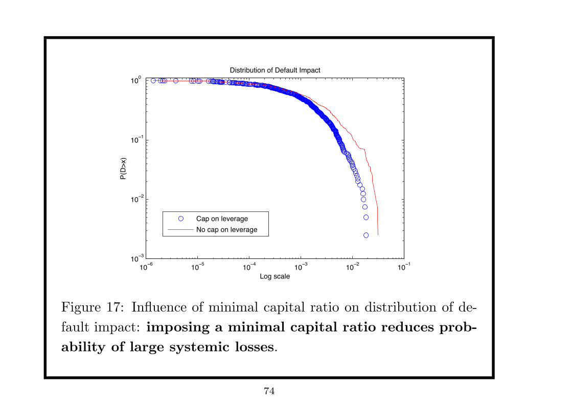
10−6 10−5 10−4 10−3 10−2 10−110−3

10−2

10−1

100

Log scale

Distribution of Default Impact

P(D

>x)

Cap on leverageNo cap on leverage

Figure 17: Influence of minimal capital ratio on distribution of de-

fault impact: imposing a minimal capital ratio reduces prob-

ability of large systemic losses.

74

0.005 0.01 0.015 0.02 0.025 0.03 0.035 0.04 0.045 0.051

2

3

4

5

6

7

8

9x 10−3

Minimal Liquidity Ratio

Max

imum

Def

ault

Impa

ct

Figure 18: The worst-case default impact decreases mono-

tonically with the minimal capital ratio: loss generated by the

institution with highest default impact as a function of the minimal

ratio of capital to total exposures.

75

Capital-e�ciency of networks

The lack of monotonicity of the Contagion Index with respect tototal capital or capital ratios leads to the question: given a networkof exposures and capital allocation, is there a better scheme ofcapital requirements/allocations which reduces systemic risk(Contagion Indices) without increasing the total level of capitalrequirements?

A capital allocation c in the network of exposures E is said to moreglobally capital-e�cient than c

0 if

X

i

c

0(i) >X

i

c(i) and 8k 2 V ,CI (k , c 0,E ) CI (k , c ,E )

Such examples exist! But they also arise in empirical data...


Capital requirements and network heterogeneity

Heterogeneity of network exposures suggests that homogeneous

capital ratios, as practiced currently, are not necessarily the moste�cient.

Also, the key role played by ’contagious links’, defined through highexposure-to-capital ratios E (i , j)/c(i), suggests that the resilience ofthe network is governed by concentration of exposures across

counterparties, which the capital ratio

�(i) =c(i)P

j 6=i E (i , j)

is not sensitive to.

This pleads for capital requirements based not just on �(i) but onthe distribution of ✓

c(i)

E (i , j), j 6= i

◆

As an example: capital requirements based on max( c(i)E(i,j) , j 6= i)


Monitoring nodes or monitoring links? A new look at capital requirements


Current prudential regulation uses as main tool monitoring and lower bounds for capital ratios defined as c(i)/A(i) where A(i)= sum of exposures of i+ other assets of i= Σj Eij +a(i) Typically a uniform lower bound is imposed on capital ratios for all institutions, regardless of their size/ systemic risk. Capital ratios do not quantify the concentration of exposures. On the other hand: Simulations show the crucial role of contagious exposures (“weak links”) with

Eij > c(i)+�i(Z) In other fields (epidemiology, computer network security,..) immunization strategies focus on - Monitoring or immunizing the most ‘systemic’ nodes -strengthening weak links as opposed to uniform or random monitoring. This pleads for monitoring links representing large relative exposures relative to capital (large value of Eij /c(i) ) In a heterogeneous network, this can make a big difference!

Capital requirements targeting ’large exposures’

Our proposal is to target (i.e. impose a lower bound on)

(i) = max(c(i)

E (i , j), j 6= i) �

min

This has the e↵ect of penalizing the concentration of exposures on afew counterparties.

Same spirit as regulatory initiatives for monitoring/limiting LargeExposures.


Targeted vs non-targeted capital requirements

We compare, in various empirical and simulated heterogeneous exposurenetworks, the impact of 4 di↵erent capital requirement schemes:(a) ’Homogeneous’ capital ratio:

�(i) =c(i)P

j 6=i E (i , j)� �

min

(b) Targeted capital ratios: higher ratios for 5% ’most systemic’institutions (SIFIs):

�(i) =c(i)P

j 6=i E (i , j)� �

min

if CI (k) � VaR(CI , 95%)

(c) Capital-to-exposure ratio for all institutions:

(i) = max(c(i)

E (i , j), j 6= i) �

min

(d) Capital-to-exposure ratio for SIFIs (5% ’most systemic’ institutions):

(i) = max(c(i)

E (i , j), j 6= i) �

min

if CI (k) � VaR(CI , 95%)


Targeted vs non-targeted capital requirements

For each scheme, we vary the threshold/limit imposed on the ratios andexamine

The aggregate capital requirement across nodesP

i c(i)

The average of Contagion Indices for 5% most systemic nodes= 5% Tail Conditional Expectation TCE (CI (c ,E ), 5%) of thecross-sectional distribution of the Contagion index.

We will consider a capital requirement c 0 = (c 0(i), i 2 V ) as moree�cient in reducing systemic risk than c = (c(i), i 2 V ) if it reduces thepotential losses from the failure of most systemic institutions withoutincreasing the aggregate level of capital requirements:

X

i2V

c

0(i) X

i2V

c(i) while TCE (CI (c 0,E ), 5%) < TCE (CI (c ,E ), 5%)


Comparison of various capital requirement policies: (a) minimum capital ratio for all institutions in the network, (b) minimum capital ratio only for the 5% most systemic institutions, (c) uniform capital-to-exposure ratio (d) capital-to-exposure ratio for the 5% most systemic institutions. (Cont Moussa Santos 2010)

Focusing on weak links: targeted capital requirements

Homogeneous vs inhomogeneous capital requirements

Targeting SIFIs with higher capital ratios may reduce theirprobability of failure but, for the aggregate level of capital, does notreduce (in fact, increases) the systemic losses conditional on a SIFIfailure.

On the other hand, a lower bound capital-to-exposure ratio has astronger mitigating e↵ect on systemic losses due to SIFI defaultsthan a simple capital ratio: it allocates capital in order to strengthenthe ’weakest links’ in the network.

Summary:

(i) focus on (weak) links, not nodes.

(ii) Heterogeneity of network structure makes homogeneous ratiosine�cient.

Currently regulators are considering the ’cover one counterparty’ rulewhich amounts to a limit of 100% on capital-to-exposure ratio.Note that enforcing such a rule does not require to observe the entirenetwork.Implementation involves other issues, in particular identification/trackingof the ultimate beneficiary in financial transactions.


Role of macro-shocks and diversification

Stress scenarios triggered by large values of a risk factor Z :

✏(i ,Z ) = c(i)fi (Z ) (6)

fi (Z ) represents the exposure of bank i to this risk factor.

Monotonicity wrt macro-shocks: greater |fi | leads to greater valuesof Contagion Index.

Contribution of macro shocks to CI (k , c ,E ) is limited to he set{i , fi (Z ).fk(Z ) > 0}: tis set is smallest in totally segmented markets,and its size increases with diversification.

Worst case: in a totally ’globalized’/ diversified market{i , fi (Z ).fk(Z ) > 0} = V

Consequence: large-scale diversification increases exposure tosystemic risk!

Diversification reduces the ’volatility’/ marginal risk measure of bankportfolios in non-stress scenarios but.. increases the probability ofjoint losses in stress scenarios generated by the common riskfactor(s) so increases the possibility of contagion.


Conclusion

Exposures across financial institutions reveal a highly concentratedand heterogeneous network structure with some highly connectedlarge nodes.

As a consequence of this heterogeneity: contagion can be triggeredby a local shock on a node yet result in largesystem-wide losses,concentrated a small sub-graph of contagious links betweencritically important nodes.

Use metrics based on conditional loss, not expected loss orprobability of contagion.

Homogeneous models may lead to incorrect insights on systemic risk.

Monitor links, not just nodes simple indicators based on theratio of the largest exposure to capital can provide a moree�cient instrument for monitoring and regulating contagion risk,without requiring a detailed observation of network structure.


Contagion in large counterparty networks: analytical results

•  Amini, Cont, Minca (2010): mathematical analysis of the onset and magnitude of contagion in a large counterparty network (n->∞)

•  Main point: contagion may become large-scale if

where µ(j,k)= proportion of nodes with with j debtors, k creditors λ = average number of counterparties q(j,k) : fraction of overexposed nodes with (j,k) links, = fraction of nodes with degree (j,k) such that at least ONE exposure exceeds capital

µ( j,k) jkλj,k

∑ q( j,k)>1

Some questions

Default impact and the amplitude of solvency cascades have been

studied by central banks via large scale simulations.

Simulation results indicate a high degree of dependence on the

structure of the network but seem difficult to generalize in absence

of further insight.

∙ How does network structure –level of capital requirements,

magnitudes and distribution of exposures– influence default

contagion in a financial networks?

∙ Which characteristics of a node/ subnetwork render it

dangerous from the point of view of systematic risk?

∙ How can contagion risk be effectively monitored by the

regulator?

19

Similar issues have been studied in mathematical epidemiology and

percolation theory either

-theoretically in a homogeneous and/or non-weighted graphs (

Bollobas et al, Janson et al, Balogh & Pittel, Wormald,...)

-using simulations or mean-field approximations (Watts & Strogatz,

Gai & Kapadia).

Most studies focus on undirected graphs.

We tackle these questions analytically, for the case of a general

heterogeneous, directed, weighted network, using asymptotics and

probabilistic methods.

20

The relevance of asymptotics

Most financial networks are characterized by a large number of

nodes: FDIC data include several thousands of financial

institutions in the US.

To investigate contagion in such large networks, in particular the

scaling of contagion effects with size, we can embed a given

network in a sequence of networks with increasing size and

studying the behavior/scaling of relevant quantities (cascade size,

total loss, impact of regulatory policy) when network size increases.

A probabilistic approach consists in

-building an ensemble of random networks of which our network

can be considered a typical sample

-showing a limit result (convergence in probability or almost sure

convergence) of the relevant quantities in the ensemble considered

as ! → ∞

21

Analysis of cascades in large networks

We describe the topology of a large network by the joint

distribution !!(", $) of in/out degrees and assume that !! has a

limit ! when graph size increases in the following sense:

1. !!(", $) → !(", $) as % → ∞: the proportion of vertices of

in-degree " and out-degree $ tends to !(", $)).

2.∑

",$ "!(", $) =∑

",$ $!(", $) =: & ∈ (0,∞) (finite expectation

property);

3. &(%)/% → & as % → ∞ (averaging property).

4.∑!

%=1((+!,%)

2 + ((−!,%)2 = )(%) (second moment property).

55

A random network model for asymptotics

To embed out networks in an ensemble of networks with increasing

size, we use the configuration model

Given a sequence of in/out degrees !+!,# and out-degrees !−!,# and

exposure matrices ("!#$), we generate a random ensemble of

networks with the same degree sequence by randomly permuting

the exposures across links going out of each node

This construction generates random networks with the same degree

sequences and same distribution of exposures, which can be both

specified from data.

56

Figure 14: Random configuration model: random matching of in-

coming half-edges with weighted out-going half-edges.

57

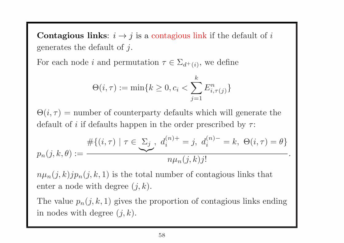
Contagious links: ! → " is a contagious link if the default of !

generates the default of ".

For each node ! and permutation # ∈ Σ!+("), we define

Θ(!, #) := min{% ≥ 0, &" <#∑

$=1

(%",'($)}

Θ(!, #) = number of counterparty defaults which will generate the

default of ! if defaults happen in the order prescribed by # :

)%(", %, *) :=

#{(!, #) ∣ # ∈ Σ$︸︷︷︸, +(%)+" = ", +(%)−" = %, Θ(!, #) = *}

,-%(", %)"!.

,-%(", %)")%(", %, 1) is the total number of contagious links that

enter a node with degree (", %).

The value )%(", %, 1) gives the proportion of contagious links ending

in nodes with degree (", %).

58

Resilience to

contagion

Amini, Cont,

Minca

The network

approach

The

probabilistic

approach

Contagion

The

asymptotic

size of

contagion

Resilience to

contagion

Amplification

of initial

shocks

Numerical

Results

Ideas of proofs

Conclusions

The intuition :branching processapproximation

Let us define

�(n,⇡, ✓) := P(Bin(n,⇡) � ✓) =nX

j�✓

✓n

j

◆⇡j(1� ⇡)n�j .

i

j2

...Default independentlywith probability ⇡

Default withprobability I (⇡) :=Pj ,k

kµ(j ,k)�

P✓ p(j , k , ✓)�(j , ✓,⇡)

1Degree (j , k) with

probability kµ(j ,k)�

Randomly chosen edge

The main idea is that, in a large network, a default cascade is well

approximated by an inhomogeneous branching process with rate

!(") :=∑

!,#

#̂($, &)!∑

$=0

'($, &, ()

binomial factor︷︸︸︷)($, ", () . (3)

which represents the fraction of defaults after one iteration in a

cascade where initially a fraction " of nodes default independently.

In particular, the contagion rate in the limit will be a fixed point of

! .

! : [0, 1] !→ [0, 1] always has a fixed point. Let "∗ be the smallest

fixed point of ! in [0, 1]:

"∗ = min{" ∈ [0, 1]∣!(") = "}.

26

Resilience to

contagion

Amini, Cont,

Minca

The network

approach

The

probabilistic

approach

Random

financial

networks

Configuration

Model

Assumptions

Contagion

Numerical

Results

Ideas of proofs

Conclusions

Assumptions on the exposuresequence

There exists a function p : N3

+

! [0, 1] such that for allj , k , ✓ 2 N (✓ j)

pn

(j , k , ✓)n!1! p(j , k , ✓).

as n ! 1. Then, p(j , k , ✓) represents the fraction of nodeswith degree (j , k) and default threshold ✓.This assumption is fulfilled for example in a model whereexposures are exchangeable arrays.

Proposition 1 (Asymptotic fraction of defaults). Under the above

assumptions:

1. If !∗ = 1, i.e. if "(!) > ! for all ! ∈ [0, 1), then an initial

default of a finite subset leads to global cascade where

asymptotically all nodes default.

∣%(&, '!, (!)∣)

"→ 1

2. If !∗ < 1 and furthermore !∗ is a stable fixed point of ", then

the asymptotic fraction of defaults

∣%(&, '!, (!)∣)

"→∑

#,%

+(,, -)#∑

&=0

.(,, -, /)0(,, !∗, /).

60

Resilience to contagion This leads to a condition on the network

which guarantees absence of contagion:

Proposition 2 (Resilience to contagion). Denote !(", $, 1) the

proportion of contagious links ending in nodes with degree (", $). If

∑

!,#

$%(", $) "

&!(", $, 1) < 1 (11)

then with probability → 1 as ( → ∞, the default of a finite set of

nodes cannot trigger the default of a positive fraction of the

financial network.

62

Resilience to

contagion

Amini, Cont,

Minca

The network

approach

The

probabilistic

approach

Contagion

The

asymptotic

size of

contagion

Resilience to

contagion

Amplification

of initial

shocks

Numerical

Results

Ideas of proofs

Conclusions

The skeleton of contagious links

The converse also holds :

PropositionIf X

j ,k

jkµ(j , k)

�p(j , k , 1) > 1,

then there exists a connected set �n

of nodes representing apositive fraction of the financial system, i.e. |�

n

|/n p! c > 0such that, with high probability, any node belonging to this setcan trigger the default of all nodes in the set : for any sequence(c

n

)n�1

such that {i , cn

(i) = 0} \ �n

6= ;,

lim infn

↵n

(En

, cn

) � c > 0.

Resilience condition:

∑

!,#

!"(#, !) #

%&(#, !, 1) < 1 (12)

This leads to a decentralized recipe for monitoring/regulating

systemic risk: monitoring the capital adequacy of each institution

with regard to its largest exposures.

This result also suggests that one need not monitor/know the

entire network of counterparty exposures but simply the skeleton/

subgraph of contagious links.

It also suggests that the regulator can efficiently contain contagion

by focusing on fragile nodes -especially those with high

connectivity- and their counterparties (e.g. by imposing higher

capital requirements on them to reduce &(#, !, 1)).

63

Resilience to

contagion

Amini, Cont,

Minca

The network

approach

The

probabilistic

approach

Contagion

Numerical

Results

Ideas of proofs

Random

Graph

Related Work

Coupling

Markov

chains

Conclusions

Contagion process as a Markovchain

Step 1 : description of contagion as a Markovchain

Let S j ,k,✓,ln

(t), l < ✓ j be the number of solvent banks withdegree (j , k), default threshold ✓ and l defaulted debtors beforeiteration t.Then (S j ,k,✓,l

n

(t), l < ✓ j) is a Markov chain.We introduce the additional variables of interest in determiningthe size and evolution of contagion :

• D j ,k,✓n

(t), the number of defaulted banks at time t withdegree (j , k) and default threshold ✓,

• Dn

(t) : the number of defaulted banks at time t,

• D�n

(t) : the number of remaining in-coming edgesbelonging to defaulted banks.

Resilience to

contagion

Amini, Cont,

Minca

The network

approach

The

probabilistic

approach

Contagion

Numerical

Results

Ideas of proofs

Random

Graph

Related Work

Coupling

Markov

chains

Conclusions

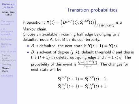
Transition probabilities

Proposition : Y(t) =⇣D j ,k,✓(t), S j ,k,✓

l

(t)⌘

j ,k,0l<✓j

is a

Markov chain.Choose an available in-coming half edge belonging to adefaulted node A. Let B be its counterparty.

• B is defaulted, the next state is Y(t + 1) = Y(t).

• B is solvent of degree (j , k), default threshold ✓ and this isthe (l + 1)-th deleted out-going edge and l + 1 < ✓. The

probability of this event is(j�l)S

j,k,✓l

(t)

m

n

�t

. The changes fornext state will be

S j ,k,✓l

(t + 1) = S j ,k,✓l

(t)� 1,

S j ,k,✓l+1

(t + 1) = S j ,k,✓l+1

(t) + 1.

Resilience to

contagion

Amini, Cont,

Minca

The network

approach

The

probabilistic

approach

Contagion

Numerical

Results

Ideas of proofs

Random

Graph

Related Work

Coupling

Markov

chains

Conclusions

• B is solvent of degree (j , k), default threshold ✓ and this isthe ✓-th deleted out-going edge. Then with probability(j�✓+1)S

j,k,✓✓�1

(t)

m

n

�t

we have

D j ,k,✓(t + 1) = D j ,k,✓(t) + 1,

S j ,k,✓✓�1

(t + 1) = S j ,k,✓✓�1

(t)� 1.

Step 2 : Law of Large Numbers : as n ! 1

Y (n⌧)

np! y(⌧)

where y(⌧) is the solution of a system of ordinarydi↵erential equations, which correspond to thenon-homogenous spatial branching process previouslydescribed.Step 3 These di↵erential equations can be solved inclosed form, yielding the stability/resilience criterion.

A measure for the resilience of a financial network •  Stress scenario: apply a common macro-shock Z, measured in %

loss in asset value, to all balance sheets in network •  The fraction q(j,k,Z) of overexposed nodes with (j,k) links is then

an increasing function of Z •  Network remains resilient as long as DEFINITION: Network Resilience = maximal shock Z* network can bear while remaining resilient to contagion Z* is solution of Given network data, Z* computed by solving single equation

µ( j,k) jkλj,k

∑ q( j,k,Z )<1

µ( j,k) jkλj,k

∑ q( j,k,Z )<1

Simulation-free stress testing of banking systems •  These analytical results may be used for stress-test the resilience

of a banking system, without the need for large scale simulation. •  Stress scenario: apply a common macro-shock Z, measured in %

loss in asset value, to all balance sheets in network •  Analytical result allow to compute fraction of defaults as

function of Z •  Network remains resilient (no macro-cascade) as long as An abrupt transition from resilience to non-resilience occurs when shock amplitude reaches Z*: cascade size/ number of defaultsas function of initial shock Z is discontinuous at Z=Z*

µ( j,k) jkλj,k

∑ q( j,k,Z )<1⇔ Z < Z *

Stress test of the international OTC dealer network (2013)


Interconnectedness and systemic risk: key insights from mathematical modeling

•  Network structure does matter when studying reisilience and stability of the finacial system: a meaningful model for financial stability should integrate network structure at level of financial institutions exposures.

•  Metrics of network resilience/ stability should make use of exposures AND capital levels and should be based on loss contagion, even in absence of default.

•  Use conditional metrics, which look at system-wide losses conditional on a loss/default/macro-event

•  Theory provides links between network structure and resilience and points to key role played by large exposures relative to capital which consitute the weak links along which contagion takes place.

•  This pleads to targeted capital requirements based on large exposures, rather than aggregate asset value. Idea: monitor ratio of large exposures to capital.

•  Network resilience varies ABRUPTLY (‘discontinously’) with the level of macroeconomic stress/shocks: onset of contagion is ‘abrupt’.

•  Beware of heterogeneity: Simple, homogeneous models may provide incorrect insights on the link between interconnectedness and systemic risk. In particular increased connectivity may increase or decrease resilience/stability, depending on network details.

!  R Cont, A Moussa, E B Santos (2013) Network structure and systemic risk in banking systems. in: Handbook of Systemic Risk, Camb Univ Press.

!  H Amini, R Cont, A Minca (2012) Stress testing the resilience of financial networks, Intl Journal of Theoretical and applied finance, Vol 15, No 1.

!  H Amini, R Cont, A Minca (2011) Resilience to contagion in financial networks, Mathematical Finance.

!  R Cont & Th Kokholm (2014) Central clearing of OTC derivatives: bilateral vs multilateral netting, Statistics & Risk Modeling, Vol 31, No 1, 3-22.

!  R Cont, L Wagalath (2012) Fire Sales forensics: measuring endogenous risk, forthcoming in Mathematical Finance.

!  R Cont, L Wagalath (2013)Running for the exit: short selling and endogenous correlation in financial markets. Mathematical Finance Vol 23, Issue 4, p. 718-741, October 2013.

!  R Cont, A Minca (2012) Credit Default Swaps and Systemic Risk, WP.

systemic risk : channels of contagion in financial systems...

Documents