what drives systemic risk? political uncertainty and ... · working paper series n. 50 june 2014...

Working Paper Series

n. 50 ■ June 2014

What Drives Systemic Risk? Political Uncertainty and Contagion in Credit Markets - "Three Essays in Empirical Finance"

Gerardo Manzo

WORKING PAPER SERIES N. 50 - JUNE 2014 ■

Statement of Purpose

The Working Paper series of the UniCredit & Universities Foundation is designed to

disseminate and to provide a platform for discussion of either work of UniCredit economists and

researchers or outside contributors (such as the UniCredit & Universities scholars and fellows)

on topics which are of special interest to UniCredit. To ensure the high quality of their content,

the contributions are subjected to an international refereeing process conducted by the

Scientific Committee members of the Foundation.

The opinions are strictly those of the authors and do in no way commit the Foundation and

UniCredit Group.

Scientific Committee

Franco Bruni (Chairman), Silvia Giannini, Tullio Jappelli, Levent Kockesen, Christian Laux,

Catherine Lubochinsky, Massimo Motta, Giovanna Nicodano, Marco Pagano, Reinhard H.

Schmidt, Branko Urosevic.

Editorial Board

Annalisa Aleati

Giannantonio De Roni

The Working Papers are also available on our website (http://www.unicreditanduniversities.eu)


Contents

Part I Political Uncertainty, Credit Risk Premium and Default Risk

Part II What Moves the Systemic Credit Risk in Europe?

Part III The Sovereign Nature of Systemic Risk (with Antonio

Picca)

THE UNIVERSITY OF ROME "TOR VERGATA"

Ph.D. in Money and FinanceXXVI Edition

What Drives Systemic Risk?Political Uncertainty and Contagion in Credit Markets

� �

"Three Essays in Empirical Finance"

by

Gerardo Manzo

SupervisorProf. Pietro Veronesi

Director of the Ph.D. ProgramProf. Gustavo Piga

Academic Year 2013-2014


.


To Mom,Dadand

Alfonso


Acknowledgements

This dissertation is the outcome of my research work at The University of Rome "Tor Vergata"

as a Ph.D. student and at The University of Chicago Booth School of Business as a visiting scholar

researcher. During this time I had the unique and rare opportunity to be supported by and to work

and share ideas with excellent professors and Ph.D students. Thus, I would like to single out the most

important of these.

First and foremost, my thankfulness and appreciation are directed to my supervisor Prof. Pietro

Veronesi, whose precious advice and guidance and scienti�c curiosity shaped my mindset positively,

forming my way of approaching the academic research. A special thank goes also to Professors Lubos

Pastor, Bryan Kelly, Stefano Giglio, Stefano Herzel and Rosella Castellano who successfully helped me

grow as a researcher. Moreover, I would also thank Professors Gennaro Olivieri and Tommaso Proietti

who were the �rst in believing in my skills as a researcher, allowing me to get into the Ph.D program.

My high gratitude goes also to the director of my Ph.D. program, Prof. Gustavo Piga, for giving me

the unique chance to work in one of the best academic environment such as the Chicago Booth School

of Business. Furthermore, I would also like to thank my colleagues and friends Ginevra Marandola,

Ugo Zannini, Emanuele Brancati and Antonio Picca for their invaluable advice and for sharing part of

my joys and sorrows during this period both in Rome and in Chicago. I also express my gratitude to

my overseas friends Bocar Ba, Princess Allen and Michael Martell for providing a friendly atmosphere,

and to my sister-in-law Alessandra for providing me excellent pictures, thanks to her graphical skills

as an architect.

My heartfelt thanks go also to my parents, Anna and Vincenzo, and to my brother Alfonso. Without

their enduring encouragement and their unrestricted faith in me, I could have never reached this great

and very important goal. A big and sincere Thank You to all these dear people who have made

everything so easy.

Rome, October 2013 Gerardo Manzo

iv WORKING PAPER SERIES N. 50 - JUNE 2014 ■

Table of Contents

Research Overview . . . . . . . . . . . . . . . . . . . . . . . . . . . . . . . . . . . . . . . . . . . . . . . . . . . . . . . . . . . . . . . . 1

Part I

Political Uncertainty, Credit Risk Premium and Default Risk . . . . . . . . . . . . . . . . . . . . . . . . . 5

1 The Data . . . . . . . . . . . . . . . . . . . . . . . . . . . . . . . . . . . . . . . . . . . . . . . . . . . . . . . . . . . . . . . . . . . . . . . . . . . . . . 10

1.1 The Geography of Credit Risk . . . . . . . . . . . . . . . . . . . . . . . . . . . . . . . . . . . . . . . . . . . . . . . . . . . . . . . 13

1.2 Principal Component Analysis . . . . . . . . . . . . . . . . . . . . . . . . . . . . . . . . . . . . . . . . . . . . . . . . . . . . . . . 14

2 Credit Risk Premium and Default Risk . . . . . . . . . . . . . . . . . . . . . . . . . . . . . . . . . . . . . . . . . . . . . . . . 16

2.1 The Pricing Model . . . . . . . . . . . . . . . . . . . . . . . . . . . . . . . . . . . . . . . . . . . . . . . . . . . . . . . . . . . . . . . . . . . 16

2.2 The Stochastic Default Intensity Process . . . . . . . . . . . . . . . . . . . . . . . . . . . . . . . . . . . . . . . . . . . . . 17

2.3 Credit Risk Premium and Default Risk . . . . . . . . . . . . . . . . . . . . . . . . . . . . . . . . . . . . . . . . . . . . . . .19

3 Estimation Strategy . . . . . . . . . . . . . . . . . . . . . . . . . . . . . . . . . . . . . . . . . . . . . . . . . . . . . . . . . . . . . . . . . . . 20

3.1 Parameters�Calibration . . . . . . . . . . . . . . . . . . . . . . . . . . . . . . . . . . . . . . . . . . . . . . . . . . . . . . . . . . . . . . 21

3.2 The Calibrated Credit Risk Components . . . . . . . . . . . . . . . . . . . . . . . . . . . . . . . . . . . . . . . . . . . . 22

4 Political Uncertainty and Credit Risk . . . . . . . . . . . . . . . . . . . . . . . . . . . . . . . . . . . . . . . . . . . . . . . . . 24

4.1 The Empirical Methodology: Panel Regressions . . . . . . . . . . . . . . . . . . . . . . . . . . . . . . . . . . . . . . 24

4.2 The Empirical Methodology: the VAR Approach . . . . . . . . . . . . . . . . . . . . . . . . . . . . . . . . . . . . 26

4.2 Exploring the Heterogeneity in the Credit Market . . . . . . . . . . . . . . . . . . . . . . . . . . . . . . . . . . . 29

5 Conclusions . . . . . . . . . . . . . . . . . . . . . . . . . . . . . . . . . . . . . . . . . . . . . . . . . . . . . . . . . . . . . . . . . . . . . . . . . . . 33

References

Tables

Part II

What Moves the Systemic Credit Risk in Europe? . . . . . . . . . . . . . . . . . . . . . . . . . . . . . . . . . . . . 49

1 Data . . . . . . . . . . . . . . . . . . . . . . . . . . . . . . . . . . . . . . . . . . . . . . . . . . . . . . . . . . . . . . . . . . . . . . . . . . . . . . . . . . 51

1.1 Commonality in the European Credit Market . . . . . . . . . . . . . . . . . . . . . . . . . . . . . . . . . . . . . . . . 54

2 Modelling Systemic Credit Risk . . . . . . . . . . . . . . . . . . . . . . . . . . . . . . . . . . . . . . . . . . . . . . . . . . . . . . . 55

v WORKING PAPER SERIES N. 50 - JUNE 2014 ■

2.1 Pricing Credit Default Swaps . . . . . . . . . . . . . . . . . . . . . . . . . . . . . . . . . . . . . . . . . . . . . . . . . . . . . . . . 56

3 Model Calibration . . . . . . . . . . . . . . . . . . . . . . . . . . . . . . . . . . . . . . . . . . . . . . . . . . . . . . . . . . . . . . . . . . . . . 58

3.1 The Unscented Kalman Filter . . . . . . . . . . . . . . . . . . . . . . . . . . . . . . . . . . . . . . . . . . . . . . . . . . . . . . . 59

3.2 Calibration . . . . . . . . . . . . . . . . . . . . . . . . . . . . . . . . . . . . . . . . . . . . . . . . . . . . . . . . . . . . . . . . . . . . . . . . . . 60

4 A Systemically Important Sovereign System . . . . . . . . . . . . . . . . . . . . . . . . . . . . . . . . . . . . . . . . . . . 63

4.1 Does Political Uncertainty Matter in Europe? . . . . . . . . . . . . . . . . . . . . . . . . . . . . . . . . . . . . . . . 64

4.1.1 A Deeper Analysis on the Political E¤ect . . . . . . . . . . . . . . . . . . . . . . . . . . . . . . . . . . . . . . . . . . 66

4.2 Is the European Crisis a Debt Crisis? . . . . . . . . . . . . . . . . . . . . . . . . . . . . . . . . . . . . . . . . . . . . . . . 67

5 Conclusions . . . . . . . . . . . . . . . . . . . . . . . . . . . . . . . . . . . . . . . . . . . . . . . . . . . . . . . . . . . . . . . . . . . . . . . . . . . 69

References

Part III

The Sovereign Nature of Systemic Risk (with Antonio Picca) . . . . . . . . . . . . . . . . . . . . . . . . . . 71

1 Introduction . . . . . . . . . . . . . . . . . . . . . . . . . . . . . . . . . . . . . . . . . . . . . . . . . . . . . . . . . . . . . . . . . . . . . . . . . . 72

2 Systemic Credit Risk Measure . . . . . . . . . . . . . . . . . . . . . . . . . . . . . . . . . . . . . . . . . . . . . . . . . . . . . . . . . 74

2.1 Tail Probability: Importance Sampling . . . . . . . . . . . . . . . . . . . . . . . . . . . . . . . . . . . . . . . . . . . . . . 75

2.1.1 Portfolio Credit Risk . . . . . . . . . . . . . . . . . . . . . . . . . . . . . . . . . . . . . . . . . . . . . . . . . . . . . . . . . . . . . . 75

2.1.2 Exponential Twisting . . . . . . . . . . . . . . . . . . . . . . . . . . . . . . . . . . . . . . . . . . . . . . . . . . . . . . . . . . . . . . 76

2.1.3 Conditional Importance Sampling . . . . . . . . . . . . . . . . . . . . . . . . . . . . . . . . . . . . . . . . . . . . . . . . . 77

2.1.4 Simulation Approach . . . . . . . . . . . . . . . . . . . . . . . . . . . . . . . . . . . . . . . . . . . . . . . . . . . . . . . . . . . . . . 78

2.2 Inputs of the Portfolio Approach . . . . . . . . . . . . . . . . . . . . . . . . . . . . . . . . . . . . . . . . . . . . . . . . . . . . 79

3 Data . . . . . . . . . . . . . . . . . . . . . . . . . . . . . . . . . . . . . . . . . . . . . . . . . . . . . . . . . . . . . . . . . . . . . . . . . . . . . . . . . . 79

3.1 Systemic Credit Risk . . . . . . . . . . . . . . . . . . . . . . . . . . . . . . . . . . . . . . . . . . . . . . . . . . . . . . . . . . . . . . . . 81

4 Empirical Framework . . . . . . . . . . . . . . . . . . . . . . . . . . . . . . . . . . . . . . . . . . . . . . . . . . . . . . . . . . . . . . . . . 83

4.1 Narrative Approach . . . . . . . . . . . . . . . . . . . . . . . . . . . . . . . . . . . . . . . . . . . . . . . . . . . . . . . . . . . . . . . . . 83

4.2 Shock Identi�cation . . . . . . . . . . . . . . . . . . . . . . . . . . . . . . . . . . . . . . . . . . . . . . . . . . . . . . . . . . . . . . . . . 84

4.3 Aggregate Results . . . . . . . . . . . . . . . . . . . . . . . . . . . . . . . . . . . . . . . . . . . . . . . . . . . . . . . . . . . . . . . . . . . 85

4.4 Portfolio Approach Sovereigns . . . . . . . . . . . . . . . . . . . . . . . . . . . . . . . . . . . . . . . . . . . . . . . . . . . . . . . 88

vi WORKING PAPER SERIES N. 50 - JUNE 2014 ■

4.4.1 Sovereigns . . . . . . . . . . . . . . . . . . . . . . . . . . . . . . . . . . . . . . . . . . . . . . . . . . . . . . . . . . . . . . . . . . . . . . . . . 88

4.4.2 Banks . . . . . . . . . . . . . . . . . . . . . . . . . . . . . . . . . . . . . . . . . . . . . . . . . . . . . . . . . . . . . . . . . . . . . . . . . . . . . 89

5 Conclusions . . . . . . . . . . . . . . . . . . . . . . . . . . . . . . . . . . . . . . . . . . . . . . . . . . . . . . . . . . . . . . . . . . . . . . . . . . . 90

References

Tables

Figures

vii WORKING PAPER SERIES N. 50 - JUNE 2014 ■

Research Overview

The wave of sovereign debt-increases, aimed at rescuing the �nancial and banking systems in Europe

after the �nancial collapse of the mid-2007, has resulted in a rapid widening of the credit spreads. Thus,

di¢ culties in rolling-over the debt on capital markets have arisen, requiring the intervention of third

parties, such as the ECB, IMF and World Bank. Indeed, speci�c events can lead to dramatic changes

in the willingness to bear sovereign credit risk, a¤ecting adversely the �nancial markets. These changes

are mostly re�ected in credit spread variations, which have their own roots in the perceived default

risk of that speci�c country. Therefore, the consequent high volatility in the European credit market

has laid the basis for analyzing the main driving macroeconomic forces.

The worsening debt situation in Europe is the point of departure of my dissertation. There has been

an increasing research on the macroeconomic determinants of the credit markets since the breakdown

of the �nancial crisis. Pan and Singleton (2008), Ang and Longsta¤ (2011) and Longsta¤ et al (2011)

are just some exemplary works of this growing literature, that shows how variations in the credit

market are signi�cantly linked to both �nancial and economic variables. My main contribution to

the literature is twofold: on one hand, I stress the role of political uncertainty in the European credit

market; on the other hand, I study the impact of bank speci�c and sovereign speci�c shocks to systemic

credit risk and analyze the contagion e¤ect between two macro systems: the European sovereigns and

the European banking systems.

During a period of �nancial turmoil, making coherent political decisions in a short time is crucial

for avoiding crisis worsening. The issue becomes more serious when the core of the discussion is a

country�s bailout such as the �rst Greek one. In fact, Greece was rescued on May 2010 after a long

period of hesitation which took about four months before the leading European economies reached

the agreement. Such a period was characterized by a high volatility, not only in the European credit

market, but also in the �nancial markets. Therefore, the Greek situation may be seen as a signal that

the EU political environment was still far from being stable. Additionally, the rapid expansion of the

Credit Default Swap market over the period 2008 to 2012 may be seen as a signal of the increasing

1 WORKING PAPER SERIES N. 50 - JUNE 2014 ■

risk aversion in the credit market.

Proxying for political uncertainty may be a hard task. To this end, I rely on the work of Baker

et al. (2011) who created a monthly index which proxies for the policy-related uncertainty in a

particular way. In fact, their index is a weighted sum of two components: newspaper coverage of

policy-related economic uncertainty and disagreement among professional economic forecasters. The

former is obtained by counting the number of articles including policy relevant terms, such as "policy,"

"tax," "de�cit", "strikes", "political uncertainty" and so on, and then detrended in order to take into

account the increasing number of news over years. Disagreement among forecasters is then used as a

proxy for uncertainty about monetary and �scal policies.

In the �rst part of this dissertation, entitled Political Uncertainty, Credit Risk Premium and Default

Risk, I study the e¤ect of political uncertainty on the credit risk premium (or distress risk) and on

the default risk (or jump-to-default risk) embedded in the term structure of sovereign Credit Default

Swap spreads over the Euro zone. The credit risk premium is the premium an investor asks to bear

the risk of that asset due to unexpected variations in the default intensity, whereas the default risk

is the (negative) jump upon default in the value of the contingent claim. After calibrating the Pan

and Singleton (2008) pricing model for sovereign CDS spreads used to obtain a spread decomposition

into two components, I �nd that the credit risk premium accounts, on average, for the 42 percent of

the observed spreads in the European credit market. Therefore, relying on a Vector Autoregressive

approach, I show how political uncertainty has a signi�cant lead-lag relation with both credit measures,

where a 10 percent increase in the degree of political uncertainty leads to a signi�cant increase in the

two components of the credit risk of about 3 percent after a month. Additionally, individual countries

react di¤erently to variations in the degree of political uncertainty, highlighting a sort of heterogeneity

in the European credit market. On an aggregate level, Impulse Response Functions shows how a shock

to the credit market, that increases the default risk, decreases the degree of political uncertainty after

three months the shock is generate. Such a result may signal the corrective or disciplinary role of the

market in putting pressure on policymakers, to act so as to reduce the political uncertainty in the

presence of a serious risk of default, rather than "mere" variations in the risk aversion. Therefore,


implementing more coherent and persuasive policies may be a signal of a more cohesive action of the

European Union that may help reducing the risk aversion in the credit market which pushes up the

funding cost for governments.

In the second part, entitledWhat Moves the Systemic Credit Risk in Europe?, I analyze the systemic

nature of sovereign credit risk in the European Union. Exploiting a cross section of 24 countries and the

Credit Default Swap term structures, I extract the systemic default intensity by calibrating the Ang and

Longsta¤ (2011) sovereign CDS pricing model using the Unscented Kalman Filter. Interestingly, the

systemic intensity reaches the highest peaks during the Lehman default and the Summer 2011, when

political issues resounded in Europe. The empirical analysis shows how variations in the probability of

a systemic breakdown are mostly driven by global stock and credit market variables. Moreover, I �nd

that political uncertainty adds up a signi�cant amount of systemic credit risk, with a lead-lag e¤ect of

one month. Finally, I �nd that higher default intensities in the European Union are associated with

higher debt over GDP and bank asset over GDP ratios. Such a linkage becomes positive and signi�cant

when the European Commission started the important debate in 2010 about the �rst bailout in the

European Union history so far. Therefore, policy interventions aimed at reducing the large debts,

at restoring growth rates and reaching a sort of political stability in the most developed European

countries may contribute signi�cantly to reduce the probability of a systemic breakdown of the whole

European Union.

In the last part of this dissertation, I introduce the joint work with Antonio Picca, entitled The

Sovereign Nature of Systemic Risk. We study the impact of bank speci�c and sovereign speci�c shocks

to systemic credit risk and analyze the contagion e¤ect between two macro systems: the European

sovereigns and the European banking systems. We form portfolios of sovereign and bank debt and,

using a Bayesian technique, we measure systemic risk as the premium an investor would pay for

hedging tail losses on those portfolios. We then identify bank speci�c and sovereign speci�c shocks

relying on the narrative approach. Channels of contagion are studied according to a portfolio sorting

approach, where we sort European sovereigns according to their debt over GDP ratios, and European

banks according to their exposure to the most leveraged countries. We mainly �nd that the system of


sovereign spreads out a sort of systemic risk that cannot be neglected, especially if we realize that the

sovereign system is ultimately in charge of bailing out the banking system. From a macro prudential

perspective as it suggests that the announcement of macro policies, aimed at mitigating sovereign

systemic risk, also have a signi�cant impact on banking systemic risk but not vice-versa. Therefore,

policies that target the sovereign system should be preferred over policies that target the banking

system.

By means of the results presented in this work, I think that the high level indebtness in Europe

signals a signi�cant degree of fragility that has to be further explored. Indeed, understanding what

moves investors� risk aversion may be of crucial importance for the policy-maker in identifying the

right strategies, in order to mitigate the systemic credit risk and corroborate the anti-fragility of a

complex system, that is, the European sovereign system.


Political Uncertainty, Credit Risk Premium and Default Risk

Gerardo Manzo�

PhD Candidate in Money and Finance

University of Rome "Tor Vergata"

� .�

Visiting Scholar Researcher

The University of Chicago Booth School of Business

� .�

Preliminary version: October 31, 2012

This version: August 31, 2013

Abstract

I study the e¤ect of political uncertainty on the credit risk premium (or distress risk ) and on the defaultrisk (or jump-to-default risk ) embedded in the term structure of sovereign CDS spreads over the Euro zone.After calibrating the Pan and Singleton (2008) pricing model for sovereign Credit Default Swap spreadsused to obtain a spread decomposition into two components, I �nd that the credit risk premium accounts,on average, for the 42 percent of the observed spreads in the European credit market. Therefore, relyingon a Vector Autoregressive approach, I show how political uncertainty has a signi�cant lead-lag relationwith both credit measures, where a 10 percent increase in the degree of political uncertainty leads to asigni�cant increase in the two components of the credit risk of about 3 percent after a month. Additionally,individual countries react di¤erently to variations in the degree of political uncertainty, highlighting asort of heterogeneity in the European credit market. Hence, this work enriches the understanding aboutthe macroeconomic forces that have driven variations in sovereign risk over the Euro zone and introducepolitical uncertainty as a signi�cant factor driving the European credit market.

[JEL No. G12, G13, G18]Keywords: Political Uncertainty, Credit Default Swap, Credit Risk Premium, Default Risk, Panel

VAR, Sovereign Debt, Term Structure

[email protected] .Gerardo Manzo is a PhD candidate in Money and Finance at the University of Rome "TorVergata". The paper was written while Gerardo Manzo was a visiting scholar researcher at The University of Chicago BoothSchool of Business. The author is grateful to Pietro Veronesi, Lubos Pastor, Rosella Castellano, Ginevra Marandola, UgoZannini, Emanuele Brancati and Branimir Jovanovic, for their invaluable comments. All errors are my responsibility.


Does political uncertainty in the Euro zone matter for investors around the world? In other words, how

is the problem-solving ability of the European leading economies perceived by �nancial investors? Does

political uncertainty a¤ect symmetrically all the European countries, or could one con�gure a regional or a

geographic e¤ect?

Speci�c events can lead to dramatic changes in the willingness to bear sovereign credit risk, a¤ecting

adversely the �nancial markets. These changes are mostly re�ected in credit spread variations, which have

their own roots in the perceived default risk of that speci�c country, whose policy depends crucially on

political decisions of the European Union. I analyze this issue through the lens of the sovereign credit default

swap (CDS) market which allows for understanding the implied default risk of a country.

During a period of �nancial turmoil, making coherent political decisions in a short time is crucial for

avoiding crisis worsening. The issue becomes more serious when the core of the discussion is a country�s

bailout. Greece was rescued on May 2010 after a long period of hesitation which took about four months.

In fact, as reported by the New York Times in an article of February 15, 2010, "...opposition grew among

Germans to bailing out what they call spendthrifts to the south after years of belt-tightening by workers at

home". During those four months, investors were worried about the uncertainty concerning the �rst bail-out

in the European Union history, such that the cumulative return, from the beginning of 2010 to the day before

making the decision (May 10, 2010), accounted for a -26.89% for the Athens Stock Exchange index (ASE) and

67.22% for the 10-year Greek sovereign bond yield. Similar variations, just slightly di¤erent in magnitudes,

were experienced also by other peripheral countries such as Ireland, Italy, Portugal and Spain.

The Greek situation may be seen as a signal that the EU political environment is still far from being

stable. The rapid expansion of the CDS market over the period 2008 to 2012 may be seen as a signal of the

increasing risk aversion in the credit market.

This study is related to the literature that explains empirically sovereign CDS spreads variations through

a macroeconomic perspective.

It is closely related to the work of Pan and Singleton (2008), Longsta¤ et al. (2011) and And and Longsta¤

(2011). The former builds a sovereign CDS pricing model which allows for the spread decomposition into a

market price of risk and a default risk. They �nd that the market price of risk of some emerging markets,

6WORKING PAPER SERIES N. 50 - JUNE 2014 ■

such as Turkey, Mexico and Korea, is statistically correlated with some measures of �nancial market volatility

(VIX), global event risk (US credit spread) and macroeconomic policy (currency-implied volatility). Longsta¤

et al. (2011) calibrate the same pricing model over a wider set of emerging markets and then regress the

CDS spread components on local and global market variables, on di¤erent measures of risk premiums, such

as equity, volatility and term premia and on global capital �ows. They �nd that CDS-implied risk premia are

more related to global economic measures than to local variables. Ang and Longsta¤ (2011) improve the Pan

and Singleton (2008) sovereign model including a systematic risk and calibrating it cross-sectionally on two

huge geographic areas, Europe and the US. Their main results are that the Euro zone shares a systematic

credit risk greater than states in the US, and that credit risk is more a¤ected by �nancial markets than by

macroeconomic fundamentals.

Researchers have been analyzing the macroeconomic determinants of sovereign CDS spreads since the

data availability has allowed for the investigation of a pure measure of credit risk. Several works have focused

their attention on the sovereign debt situation in the Euro zone. Sgherri and Zoli (2009) analyze empirically

the determinants of the common time-varying factor implicit in the credit spread of 10 EU economies over the

period January 1999 to April 2009. They �nd that this factor is positively correlated with volatility in stock,

currency and emerging markets. Dieckmann and Plank (2009) study the determinants of CDS spreads during

the mid-2007 �nancial crisis for 18 European developed economies. They argue that the size and the pre-crisis

health of both the world and country�s �nancial market positively a¤ect the CDS spread. Moreover, they

stress the potential role of the private-to-public risk transfer channel - that is, more government guarantees

on the �nancial sectors, signi�cant extension of loans�amount to the banking system, etc. - which allows

investors to form expectations about future �nancial bailouts. Related to this work is Acharya et al. (2011)

which �rst models and then tests the two-way feedback e¤ect between the sovereign credit risk and �nancial

markets. When a sovereign comes into play to rescue its insolvent �nancial system with a debt expansion

�nanced by taxes, it induces a positive signal in the market which then turns into a negative one owing

to an increase in the marginal cost of raising the tax revenue (La¤er curve) and a more limited maximum

debt capacity. Hence, a distressed sovereign may exacerbate the �nancial sector�s solvency condition since it

would no longer be able to make any transfer. Another interesting study has been conducted by Brutti and


Sauré (2012) who assess the contribution of �nancial linkages to the transmission of sovereign default risk.

Thanks to a particular econometric tool, they are able to identify �nancial shocks that originated in Greece

and spread overall European countries. They �nd that "a 10 percent increase in the exposure to Greek debt

increases the rate of cross-country transmission of sovereign risk by 3.94 percent".

Alongside empirical studies on the macro-determinants of credit spread, theoretical and empirical works

on the role of political decisions in both stock and capital markets have recently been developed. Pastor and

Veronesi (2011a), Pastor and Veronesi (2011b) and Ulrich (2011), among others. The former theoretically in-

vestigates the e¤ect of the government�s policy decision on the stock prices in a Bayesian-learning equilibrium

framework. Their main result is that, on average, the stock price drops down, with this reduction being larger

when the announcement of a political change includes elements of surprise. Pastor and Veronesi (2011b)�s

model allows for the equity risk premium�s decomposition into three components related to three di¤erent

shocks. While the �rst two are deemed as economic shocks, the third one is the political shock which "a¤ect

investors�beliefs about which policy the government might adopt in the future". Moreover, using the Baker

et al. (2011)�s policy-related uncertainty index, they �nd empirical evidence that political uncertainty is

state-dependent, since it is higher when worse economic conditions are in play. Lastly, Ulrich (2011) analyze

the e¤ect of political uncertainty on the bond market through a pricing model that incorporates political

uncertainty. The latter regards the Ricardian equivalence uncertainty (or Knightian uncertainty), according

to which investors expect a non-zero consumption growth rate after the implementation of a government

policy. The model predicts that a government policy a¤ecting the business cycle leads to a positive risk

premium for investors.

My work introduces a novelty in the literature. To my best knowledge, it is the �rst in investigating the

linkage between implied-CDS risk premium and political uncertainty. While the former requires a theoretical

framework to be extracted from asset prices, it is challenging to measure the degree of political uncertainty

over time. As a result, Baker et al. (2011) have created a monthly index able to proxy for policy-related

uncertainty over time.

The analysis is conducted on a sample of 19 European countries, inside and outside the EU and EMU.

For each country, I calibrate the Pan and Singleton (2008) pricing model for sovereign CDS to decompose


the spread into the two components: the credit risk premium and the default risk. The former measures the

compensation investors demand for bearing the credit risk of that country due to unexpected variations in

the default intensity, namely, the probability of default, whereas the default risk is a residual measure that

is a proxy for the (negative) jump in the value of the contingent claim upon default. Several results emerge

from this analysis.

First, I �nd that the sovereign CDS market embodies credit risk features that allow countries to live in

di¤erent clusters. In fact, the Cluster Analysis shows a certain geography of the credit risk, where the biggest

group is comprised of the most e¢ cient economies or core economies, such as Austria, Finland, France,

Germany, Netherlands, Sweden and UK. Two more distinct groups are formed: the most worrying countries

or peripheral economies, such as Italy, Spain, Portugal, Ireland and Belgium1 and the Eastern countries, such

as Estonia, Romania, Latvia, Lithuania and Poland. In two di¤erent and very distant clusters are Greece

and Norway, deemed the riskiest and the safest countries of Europe, respectively.

Second, a principal component analysis, performed on the correlation matrix of daily variations of CDS

spreads, reveals commonality across countries and regions. It is done across the three macro European

regions as from the clusters�composition. On one hand, when the full sample is considered, the �rst three

components explain the 84 percent of the variability, which becomes higher (over 90%) when the clusters

are examined individually. Univariate regressions shows how the variations in the �rst PCs are signi�cantly

related to political uncertainty as well as European and US �nancial variables.

Third, alongside Pan and Singleton (2008) and Longsta¤ et al. (2011)�s works, the model calibration shows

that the credit environment is worse under the risk-neutral probabilities than under the objective probabilities

and provides larger and more persistent default intensities. Additionally, the credit risk premium accounts,

on average, for the 42 per cent of the observed Credit Default Swap spread.

Fourth, panel regressions of the variations in the credit risk premia show how a 10%-increase in political

uncertainty, after controlling for information already included in both the European and the US �nancial

markets, leads to a signi�cant increase in the credit risk premia of about 3.2 percent after a month. Such an

increase is slightly smaller in the case of the default risk, that is, 2.9 per cent but still signi�cant. Moreover,

1Belgium is included among the unstable countries since it has gone through a period of political instability from 2007 to2011. A point which will be clearer later on.


relying on a panel vector autoregressive (VAR) approach, I con�rm the signi�cant lead-lag relation of political

uncertainty with both the credit risk premia and the default risk. On an aggregate level, a shock to the credit

market that increases the default risk decreases the degree of political uncertainty after three months the

shock is generate. Such a result may signal the corrective or disciplinary role of the market in putting pressure

on policymakers to act so as to reduce political uncertainty in the presence of a serious risk of default rather

than "mere" variations in the risk aversion. Additionally, employing the VAR approach on a country level, I

explore the heterogeneity of the European countries�credit market in responding to variations in the degree

of political uncertainty and how the latter is in�uenced by the credit conditions of speci�c countries such

as the core and peripheral economies. Lastly, aggregating both the credit risk premia and the default risk

measures across the three macro regions, an interesting scenario emerges: a political shock has a signi�cant

impact on the risk premia of the peripheral economies after a month the shock is generated and on the default

risk of the core economies after three months, whereas a shock to the premia of the core economies leads to

an signi�cant increase in the degree of political uncertainty after two months. Moreover, the corrective role

of the market is con�rmed also on a regional level.

The remainder of the paper is organized as follows: Section 1 introduces description of the data, together

with the cluster analysis and the principal component analysis. The Pan and Singleton (2008) sovereign CDS

pricing model is shown in Section 2 as well as the way the credit risk premium and default risk measures

are extracted. Then, in Section 3, I calibrate the model, and, in Section 4, I stress and discuss the role of

political uncertainty in the credit market. Section 5 concludes the analysis.

1 The Data

Two types of data are used for the analysis: Credit Default Swap spreads and the European policy-related

uncertainty index.

A CDS is a �nancial derivative contract agreed between two parties: the buyer and the seller. The former

commits himself to a periodic payment, usually quarterly or semiannual, to the seller and is compensated on

the arrival of a speci�c credit event related to an underlying debt obligation such as a bond or a loan. While


for a company a credit event may be the bankruptcy or default, for a country it is not correct to talk about

a pure default. The most appropriate de�nition for sovereign credit event is provided by the International

Swaps and Derivatives Association (ISDA), which references four types of credit events: acceleration, failure

to pay, restructuring and repudiation. As pointed out by Pan and Singleton (2008), these events cannot

happen simultaneously, and, therefore, the contract may be executed as soon as one of them occurs2 .

CDS spreads are collected from the Markit database and cover a period of 1336 days from December 3,

2007 to January 22, 2013 for the maturities 1, 3, 5, and 7 and for 19 European countries, inside and outside

the European Union and the Economic and Monetary Union. Therefore, the total dataset consists of 101,536

daily spreads. The sample period is dictated by the data availability. Indeed, trading on CDS spreads of the

wealthiest countries, such as Norway, Sweden and Germany, is not available before our starting date since the

biggest worries about the debt situation have been in the game after the bankruptcy of Lehman Brothers,

which involved sharp increases in the spreads.

The European policy-related economic uncertainty index, provided by Baker et al. (2011), is a weighted

sum of two components: newspaper coverage of policy-related economic uncertainty and disagreement among

professional economic forecasters. The former is obtained by counting the number of articles including policy

relevant terms, such as "policy," "tax," "de�cit" and so on, and then detrended in order to take into account

the increasing number of news over years. Disagreement among forecasters is used as a proxy for uncertainty,

as has already been explored by authors such as Boero et al. (2008), Bomberger (1996) and Lahiri and Sheng

(2009), among others. Baker et al. (2011) utilize individual level forecasts regarding consumer prices and

federal government budget balances since they are directly in�uenced by monetary policy and �scal policy

actions. Then, these two components are standardized and added up in order to form a monthly index3 .

I consider Austria, Belgium, Estonia, Finland, France, Germany, Greece, Ireland, Italy, Netherlands,

Portugal, and Spain, as member of both the EU and the EMU, Latvia, Lithuania, Poland, Romania, Sweden

and UK as part only of the EU, and, �nally, Norway as an extra-EU and- EMU state, deemed the safest

country in all of Europe. In order to have a picture of European countries�performances over the concerning

2The literature has been focusing on CDS spreads instead of bond spread because they are not a¤ected by both �ight-to-quality e¤ect and contractual arrangements, such as seniority, coupon rates, guarantees and embedded options.

3 Index source: www.policyuncertainty.com for additional details.


period, Figure 1 depicts the average of the changes of the unemployment rate and the mean real GDP growth

rate over the period December 2007 to January 2013 for each country.

8

6

4

2

0

2

4

6

8

10

Austria [68.8]

Belgium [95.2]

Estonia [5.85]

Finland [42.1]

France [78.2]

Germany [74.4]

Greece [132.1]

Ireland [72.3]

Italy [115.4]

Latvia [32.2]

Lithuania [29.0]

Netherlands [59.5]

Norway [41.4]

Poland [51.3]

Portugal [87.8]

Romania [24.0]

Spain [54.2]

Sweden [38.4]

UK [67.8]

Austria [68.8]

Belgium [95.2]

Estonia [5.85]

Finland [42.1]

France [78.2]

Germany [74.4]

Greece [132.1]

Ireland [72.3]

Italy [115.4]

Latvia [32.2]

Lithuania [29.0]

Netherlands [59.5]

Norway [41.4]

Poland [51.3]

Portugal [87.8]

Romania [24.0]

Spain [54.2]

Sweden [38.4]

UK [67.8]

∆UnempReal GDP Growth

Figure 1. Performances of 19 European economies in terms of unemployment rate and real-GDP growthover the period 2007 to 2013. �Unemp is the average of changes in the quarterly unemployment rate fromthe last quarter of 2007 to the second quarter of 2012. Real �GDPgrowth is averaged yearly over theperiod 2007 to 2013, where the last observation is a forecast. Average Debt over GDP ratios in brackets.

The emerging picture points out the structural di¤erences faced by each country, with the peripheral

economies, such as Greece, Italy, Portugal and Spain, showing the worst performances.

Table 1 shows summary statistics of both 5-year spreads and the policy-related uncertainty index. All

the spreads are in basis points and, even if their underlying notional is in US dollars, they are free of units

of account. The polar mean values are those of Greece and Norway, that is, over the sample period the

protection buyer would pay, on average, 1391 bps per year to hedge against the Greek default risk, while

investors are willing to pay just 21 bps to protect themselves against a remote Norwegian default. Again,

the largest standard deviation is that of Greece, followed by Ireland and Portugal. The whole picture that

emerges from this summary indicates that there is a consistent time variation in CDS spreads. The last row


reports descriptive statistics for the policy-related uncertainty index.

1.1 The Geography of Credit Risk

Given the large number of countries used for the analysis, it may be worthwhile to check if they share some

particular features such that they can live in clusters. Indeed, as shown by Figure 1, some economies share

common features, such as the peripheral ones (Italy, Portugal, Spain Ireland and Greece) and the Eastern

countries (Estonia, Latvia, Lithuania, Poland and Romania).

I perform a multivariate cluster analysis according to the complete method. Such a method is applied in

the hierarchical cluster analysis whose purpose is to optimize an objective function which is usually a distance

between a pair of clusters. Starting with each variable being a cluster, a cluster is formed at each new step

such that the variation of the within-group variance, or the distance between cluster centers, is as small as

possible, while the between-group variance is as large as possible. The algorithm uses the largest distance

between objects in the two clusters. In this case, the distance is Euclidean and measures the similarity by

computing the square root of the sum of the squared di¤erences in the variables�values.

The cluster analysis is known to be performed according to several methods (or algorithms) and distances.

Therefore, the choice is rationally dictated by the cophenetic correlation which measures the faithfulness of

the pairwise distance between the original variables�values. In other words, the higher this correlation, the

better the solution�s quality.

First of all, I use the correlation matrix of daily changes of CDS spreads as a measure of similarity among

objects. Then, I apply the method through an algorithm that attempts to form clusters at each step as

indicated above. Moreover, such a method requires knowing the number of clusters a priori ; therefore, I use

a rule of thumb and select N=4 groups, where N is the number of variables.

Table 2 shows the cluster�s composition over di¤erent periods. As expected, some European regions share

common features. Over the full sample (Panel A), the largest cluster contains the core economies (Austria,

Finland, France,Germany, Netherlands, Sweden and UK), the most worrying or peripheral economies�cluster

(Belgium, Ireland, Italy, Portugal and Spain), the cluster of Eastern countries (Estonia, Latvia, Lithuania,

Poland and Romania), and �nally, Norway and Greece in two di¤erent and far groups. These two one-item


groups con�rms the polarity of their own credit risk. Indeed, Norway that is deemed the safest European

country, has an average surplus and debt of 13.6 and 41.1, respectively, as a percentage of GDP over the period

2008-2011, while Greece is the �rst European country that has experienced a default after the constituency

of the currency union. In fact, it has an average de�cit and debt over GDP of 11.2 and 138.2, respectively,

over the period 2008-2011. Thus, I name these two as polar economies.

The biggest and primary concerns about the debt situation in the Euro zone exacerbated early in 2010

when rising government de�cits and debt levels together with a lot of companies�and sovereigns�downgrades

led the European Finance Ministers and the IMF to approve a huge monetary rescue package for Greece, and

lay basis for a deeper �nancial stability, creating the EFSF. Therefore, the Greek bailout can be considered

as the biggest main event of the European debt crisis. According to this view, I divide the sample into two

sub-periods in order to �gure out whether this event has changed the credit risk composition in the Euro

zone. Panel B of Table 2 illustrates the clusters over the period December 3, 2007 to May 2010, when the �rst

rescue package was approved, while Panel C from the end of May 2010 to March 2012. I can see a di¤erent

composition except for the Eastern countries which still share common credit risk features. It is interesting to

note that the extra-EU country, Norway, always maintains a great distance from the rest of Europe. Greece

comes out of the cluster of the peripherals due mostly to its orderly default, that is, the agreement reached

by the majority of private sovereign bondholders on March 9th, 2012 which led to the suspension of trading

on Greek CDS contracts. In addition to this, Table 2 reports also the cophenetic correlation which ensures

the goodness of the �t.

1.2 Principal Component Analysis

The Principal Component Analysis (PCA) will help measuring the degree of heterogeneity in the European

credit market. The PCA is performed on the correlation matrix of monthly log-changes of 5-year CDS

spreads. Starting from daily observations, I pick up the mid most available spread of the month ending

up with a monthly time series of 61 observations. The mid observation is chosen such that the sample is

not a¤ected by stale observation. Moreover, the log-transformation allows for scaling the very large Greek

spreads.


The emerging correlation structure, not reported here, shows that almost 26 percent of the pairwise

correlations is greater than 80 percent. This is common especially among the core economies, e.g., France

and Germany, which have a correlation of 86 percent. Moreover, Greece and Portugal present the lowest

average correlations of 12 percent and 0.8 percent, respectively.

Bearing this comovements�picture in mind, Table 3 reports the variance explained by the PCs across

both the whole set of countries and the above clusters. The table illustrates that, over the full sample (Panel

A) the �rst three components explains almost 84% of the variability of sovereign CDS spreads changes, which

becomes bigger if performed across clusters. Indeed, the �rst three PCs explain the 91.2, 91.1 and 96.1 per

cent for the Peripheral, the Core and the Eastern economies, respectively.

It may be worth notice that the �rst PC of the cluster of the Peripheral economies is only 3.8 per cent

bigger than that of the whole set of countries. Such a small di¤erence may be associated with the negative

correlation between Ireland and Portugal over the last part of the sample, when on July 21, 2011 a draft

statement drawn down by EU countries was approved, allowing the Irish government to pay a smaller interest

rate on its bailout on a longer maturity4 . This involved a trend inversion for Irish CDS spread.

Panel C of Table 3 reports univariate regressions of the �rst-di¤erences of the �rst PCs for each cluster

and for the whole set of 19 countries (Europe19). Interestingly, political uncertainty is positively and signif-

icantly related to the the �rst PCs of the three clusters with a stronger relation with the Core economies. In

addition to this, all these variables are signi�cantly related to the �rst PCs with the global market having

the strongest relation. Both the �nancial uncertainty in the European stock market (V2X) and the cred-

itworthiness of the European industrial sector (iTraxx) are signi�cantly and positively related to the �rst

PCs. Moreover, spillover e¤ect from both the US �nancial market (VIX) and the US industrial sector (IG

CDX) are signi�cantly related to the credit risk in Europe. The TED spread is signi�cant for the Eastern

economies. This result is in line with the view that Eastern economies su¤er the most liquidity problems

since their non-well developed banking systems force them to rely heavily on foreign borrowing, especially

from the biggest US banks.

The whole picture that emerges from this statistical analysis is that CDS spread variations embed credit

4Up to that day, Ireland had paid an average interest rate of 5.8% with a maturity of 7.5 years. The new agreement statedan interest rate of 3.5% and doubled the maturity.


risk features that can be clustered over speci�c European regions and that there is a certain correlation

structure with political uncertainty and other European and US �nancial variables which lay the basis for a

deeper understanding. In fact, the next goal is to test the e¤ect of political uncertainty on what moves the

European credit market, namely, the credit risk premium and the default risk, after controlling for information

already embedded in the �nancial markets.

2 Credit Risk Premium and Default Risk

This section is preliminary for the empirical analysis since here I �rst present and then calibrate the Pan and

Singleton (2008) pricing model for sovereign CDS to extract the main variables for the empirical analysis,

namely, the credit risk premium and the default risk. Once again, the credit risk premium is the premium

an investor asks to bear the risk of that asset due to unexpected variations in the default intensity, whereas

the default risk is the negative jump upon default in the value of the contingent claim.

2.1 The Pricing Model

Even if a CDS contract written on a company�s bond di¤er from that written on a sovereign bond in its own

credit event de�nition, the theoretical pricing framework is still valid. Here I report a brief description of the

Pan and Singleton (2008) reduced-form model for sovereign CDS spreads.

A CDS contract with maturityM consists of two components, the buyer�s premium, de�ned as CDSt (M)

and paid quarterly or semiannually, and the amount the buyer gets from the seller upon a credit event occurs.

Assuming a semiannual payment and a notional equal to one, the premium leg, that is, the present value of

the premium �ows, is as follows

1

2CDSt (M)

2MXj=1

EQthe�

R t+:5jt (rs+�Qs)ds

i

where the term in brackets catches the risk-neutral survival-dependent nature of the payments, that is,

they are discounted according to a risk-free interest rate, rt, plus a default intensity, �Qt5 . Instead, the present

5 In reduced-form models, a default is modeled as the �rst arrival of a risk-neutral Poisson process whose stochastic intensityprocess is represented by �Qt . For more details, see Bielecki and Rutkowski (2002).


value of the amount the seller will pay upon a credit event is

LQZ t+M

t

EQth�Que

�R ut (rs+�

Qs)ds

idu

where LQ = 1�RQ is the loss given default, expressed as the face value minus the recovery rate, RQ.

As a plain IRSs, a CDS contract is written by both the buyer and the seller if it is worth zero at inception.

This allows us to infer the contract-implicit spreads as follows:

1

2CDSt (M)

2MXj=1

EQthe�


i=�1�RQ

� Z t+M

t

EQth�Que

�R ut (rs+�

Qs)ds

idu

CDSt (M) =2�1�RQ

� R t+Mt

EQth�Que

�R ut (rs+�

Qs)ds

iduP2M

j=1 EQt

he�


i (1)

According to the way one interprets the fractional recovery, the pricing model can be di¤erent. Following

Du¢ e and Singleton (2003), Pan and Singleton (2008) and Longsta¤ et al. (2011), I assume the fractional

recovery of face value (RFV), which, under the independence assumption between the intensity of default

and interest rate, allows for the expectation�s splitting, that is,

Z t+M

t

EQth�Que

�R ut (rs+�

Qs)ds

idu '

Z tM

t

EQthe�

R ut(rs)ds

iEQth�Que

�R ut (�

Qs)ds

idu

=

Z tM

t

D (t; u)EQth�Que

�R ut�Qsds

idu

where D (t; u) represents the price of a default-free zero coupon bond issued at time t and maturing at

time u, while the expectation term is nothing more than the risk-neutral death probability.

2.2 The Stochastic Default Intensity Process

The Pan and Singleton (2008) model is challenging for its assumption about the intensity process.

They assume that the arrival rate of a credit event, �Qt , follows a Black-Karasinski lognormal stochastic

process, whose conditional expectation is known not to have a closed-form solution, since the seminal work


of Black and Karasinki (1991).

The stochastic process, under the objective probabilities, has the following representation

d ln�Qt = kP��P � ln�Qt

�dt+ ��Qt

dBPt (2)

where kP is the mean reversion speed, �P the long-term mean level and ��Qt the local volatility for local

changes in ln�Qt .

Assuming an a¢ ne market price of risk �t,

�t = �0 + �1 ln�Qt (3)

the Girsanov theorem shows that under an equivalent change of measure, the stochastic process under

the risk-neutral probability becomes

d ln�Qt = kQ��Q � ln�Qt

�dt+ ��Qt

dBQt

with kQ = kP+�1��Qt and kQ�Q = kP�P��0��Qt preserving the same characteristics as under the objective

measure.

In order not to be confused about the notation, here I am considering the risk-neutral default intensity,

�Qt , under both probability measures. The reason why I deal with such a probabilistic framework is readily

shown by Yu, Fan (2002) who, analyzing such reduced-form pricing models, points out how they can only be

applicable prior to default, since they su¤er a survival bias, which is related to the process under the objective

measure6 . Therefore, the Pan and Singleton (2008) model is able to extract only the default risk premium

(or credit risk premium or distress risk), which is the compensation investors demand for bearing the risk

due to unexpected variations in the default intensity. It does not catch the default event risk premium (or

default risk or jump-to-default), that is, the (negative) jump in the value of the contingent claim at default.

As highlighted by Longsta¤ et al. (2011), the latter is typically measured as the ratio between the risk-

6This problem emerges when the default intensities under both measures are not asymptotically equivalent, allowing for adistinction between default risk premium and default event risk premium.


neutral and the objective intensity, �Qt =�Pt . However, the objective intensity is hard to infer from prices alone

because, being a rare event, it requires deeper understanding of the �nancial situation of a sovereign. Thus,

from market prices one is able to infer only the risk-neutral intensity under the objective probabilities.

Such a lognormal process has its own advantages. Indeed, as we know, a lognormal distribution has

fatter tails than the classical noncentral chi-squared distribution of the usually-used CIR process. Even if it

preserves the mean reverting feature, is strictly positive and has a distribution skewed to the right, it may

su¤er the explosion problem. But the main shortcoming is that the outcoming survival probabilities are not

available in closed-form.

Given the intensity dynamics as described by the SDE in equation 5, the risk-neutral survival probability

EQthe�

R ut�Qsds

iis measured by approximating numerically its corresponding PDE with a fully implicit �nite

di¤erence method7 .

2.3 Credit Risk Premium and Default Risk

This model can only infer the distress risk from CDS spreads. Such a risk may be priced in the market to

the extent that the implied risk-neutral probabilities di¤er from the objective ones, which catch investors�

expectations in the sovereign CDS market.

Therefore, following Pan and Singleton (2008) and Longsta¤ et al. (2011), I estimate CDS spreads under

the objective probabilities, also known as the pseudo CDS spread, this is,

CDSPt (M) =2�1�RQ

� R t+Mtt

EPh�Que

�R ut (rs+�

Qs)ds

iduP2M

j=1t EPhe�


i (4)

where the expectations are taken under the natural probabilities.

Accordingly, the market price of distress risk premium or credit risk premium, CRPt (M), is measured

simply by the di¤erence between the CDS spread under Q in equation 1 and the pseudo one in equation 4,

7A numerical approximation, like �nite di¤erence methods, may lose stability at boundaries when the underlying processturns out to be pure convection (drift equal to zero) or pure di¤usion (volatility equal to zero). In order to avoid this, I applythe exponential �tted scheme which has good convergence properties and does not allow for spurious oscillations. For moredetails, see Du¤y (2001)


that is,

CRPt (M) = CDSt (M)� CDSPt (M) (5)

What here I call default risk is nothing more than the residual from the distress risk. In other words,

following the interpretation of the expected return given by Yu (2002), the risk premium deriving from the

di¤erence between a defaultable and a default-free bond, consists of the sum of two parties: the �rst is related

to variations in the spread, namely, in the unpredictable intensity (distress risk) and the second is related to

the default event (jump-to-default risk). Estimating the default event risk premium requires not only market

prices but also �nancial statement data, thus, following Longsta¤ et al. (2011), I quantify it as the di¤erence

between the CDS and its implicit CRP.

3 Estimation Strategy

The model is calibrated according to the quasi-maximum likelihood (Q-MLE) method, using the term-

structure of CDS spreads for the maturities 1-, 3-, 5- and 7-year. The approach is widely used in the term

structure literature and is referred to the dated works of Longsta¤ and Schwarts (1992) and Chen and Scott

(1993), and to the recent works of Du¤ee (2002), Pan and Singleton (2008) and Longsta¤ et al. (2011).

The underlying assumption is to assume that a CDS contract over a speci�c maturity is priced without

error. In such a way, one can invert the model and get the latent variable, that is, the unobservable default

intensity. This is possible thanks to the availability of a term structure of CDS spreads. A widely used

empirical trick is to choose the most liquid maturity and thus, I choose the 5-year CDS spread whose trading

volume has always been higher than other maturities8 .

The parameters are estimated with respect to the distribution of the implied-CDS default intensity. The

intensity, given by the SDE in equation 2 under the objective probabilities, has a lognormal density with

8Longsta¤ et al. (2011) argues that "We spoke with several sovereign CDS traders to investigate this [liquidity] issue. Thesetraders indicated that the liquidity and bid-ask spreads of the one-year, three-year, and �ve-year contracts are all reasonablysimilar, although the �ve-year contract typically has higher trading volume."


mean, mt, and variance, v:

m�t = ln��Qt�1

�e�k

P�t +�P

kP

�1� e�k

P�t�

v�t =�2�Qt

2kP

�1� e�2k

P�t�

Letting CDSt (M) be the vector of CDS spreads9 for maturities M = 1; 3; 7, I assume that the pricing

error � is normally distributed with mean zero and constant variance. Therefore, the model CDSt (M) =

h��Qt

�+ �t, where h (�) is the pricing function (equation 1) and �t the pricing error, is jointly estimated

according to the following joint density

fP��Qt ; �tjFt�1

�= fP

��Qt jFt�1

�� fP

��tj�Qt ;Ft�1

�= fP

��Qt j�

Qt�1

�� fP

��tj�Qt ;Ft�1

�

where the �rst term on the RHS comes from the Markov assumption of the stochastic process and

fP��tj�Qt ;Ft�1

�s N (0;), where = diag f� (1) ; � (3) ; � (7)g.

Finally, the parameter set consists of 8 parameters, that is, ��Qt ; kQ�Q; kQ; kP�P; kP; � (1) ; � (3) ; � (7).

The daily risk-free discount functions are bootstrapped from constant maturity bonds collected from the

H.15 release of the Federal Reserve system. Several methods can be used for getting discount functions

from market data, but their e¤ect in pricing CDS contract is negligible, since it enters the pricing function

symmetrically. Moreover, as shown by Du¢ e (2003), under some speci�c conditions, a CDS contract can be

replicated by an arbitrage-free portfolio by buying a default-free �oater and shorting a defaultable �oater. As

we know, the sensitivity of these securities to interest rate variations is very small, endorsing the assumption

about the method used to extract the discount function.

3.1 Parameters�Calibration

Table 4 reports the estimated parameters with standard errors in parentheses and average log-likelihoods10 .

9The pricing function is adjusted in order to account for the accrued credit-swap premium at default.10Given the large number of parameters, I set the algorithm�s convergence criterion equal to 10�17 in order to o¤set the

starting value problem. Standard errors are computed numerically.


As we can observe from the standard deviations, the model �ts the term structure well enough with some

exceptions for the 1-year CDS contract. This is a model�s feature already observed in Pan and Singleton

(2008) where the shorter maturities seem to be priced with greater errors. Moreover, the calibration con�rms

other empirical characteristics: the credit environment is worse under the risk neutral probabilities than

under the objective ones, kQ�Q > kP�P, allowing for larger and more persistent (kQ > kP) default intensities

under Q than under P for the majority of countries. Finally, kP > 0 for each country, meaning that the

process �Qt is P-stationary.

3.2 The Calibrated Credit Risk Components

Di¤erences in the calibrated parameters across probabilistic environments allow for inferring that a credit

risk premium is priced in the CDS market.

The credit risk premium for the 5-year CDS spread is computed as in equation 5. Table 5 reports summary

statistics for both the credit risk premia (CRP) and the default risk (DRP).It is worth notice that the mean

value goes from a minimum of 0.3 bps for UK to a maximum of 303.3 bps for Greece, whereas the default

risk ranges from a minimum of 8 bps of Norway to a maximum of 1142 bps of Greece. The default risk is on

average greater in magnitude than CRPs. This bigger magnitude is due to the way the default risk measure

is built. On one hand, being a residual measure, one may conclude that it can contain everything (more than

the default risk itself) except the credit risk premium. But, on the other hand, the theoretical issue explained

above asserts that it may be indeed deemed as a reliable measure of the jump-to-default risk, which is not

directly captured by reduced form models. In addition to this, the credit risk premium, on average, accounts

for a 42 per cent of the Credit Default Swap spread in Europe. In order to have a broader view of the CRP�s

evolution over time, Figure 2 plots four panels where countries are grouped in clusters as shown in Section

1.1.


Nov06 Aug09 May12 Feb150

20

40

60

80

100

120

140Core Economies

AustriaFranceNetherF inlandGermanSwedenUK


200

400

600

800

1000

1200Peripheral Economies

BelgiumItalyPortugalSpainIreland


50

100

150

200

250

300

350

400Eastern Economies

EstoniaLatviaLithuaniaPolandRomania

Jan00 May01 Sep02 Feb040

10

20

30

40Polar Economies

0

2000

4000

6000

8000GreeceNorway

Figure 2. Credit Risk Premium (CRP) extracted from the country speci�c Credit Default Swap termstructure by calibrating the Pan and Singleton (2008) Sovereign CDS pricing model. The CRPs are

grouped into three macro regions according to the outcome of the Cluster Analysis: Core, Peripheral andEastern Economies plus the group-stand-alone Polar Economies. Daily sample period December 3, 2007 to

Janury 22, 2013.

This graphical perspective con�rms that the sample can be readily split into two sub-periods, the Lehman

Brothers�bankruptcy and the Euro zone debt crisis. During these two sub-periods, all the economies expe-

rience large variations in the CRP, recording spikes of di¤erent magnitudes. While for the core economies

the CRP variations around the two macro events are comparable in magnitudes, the Eastern and peripheral

economies show opposite paths, with the formers much more a¤ected by the Lehman default rather than the

Euro debt crisis. Such a result may support the view that the European Union has di¤erent speeds, not only

for what is concerned with the growth rate or in�ation rate, but also for the perceived credit risk, allowing

for asymmetric e¤ects stirred up by a common shock that makes ine¢ cient a common policy intervention.

Moreover, as outlined by the PCA results, the Eastern countries have su¤ered the most shocks from the

�nancial crisis since these are economies with non-well developed banking systems that are forced to rely on

foreign borrowing, thus, exposed to spillover e¤ect.


4 Political Uncertainty and Credit Risk

Does political uncertainty a¤ect the risk perceptions of investors in the European credit market? In other

words, do investors require a higher risk premium in the presence of a higher degree of political uncertainty?

Is the default risk a¤ected by such an uncertainty?

I answer these questions by employing a set of panel regressions where I regress separately the two

components embedded in the credit market on the policy-uncertainty index adding step-by-step �nancial

control variables. The latter have the following purposes: �rstly, they make the analysis more robust in

case I can con�gure a signi�cant relation between political uncertainty and credit market; secondly, they

can dampen the main criticism on the policy-related uncertainty index, that is, the way it is built allows for

catching also economic and �nancial uncertainty rather than only political uncertainty. In fact, including

stock, credit and commodity markets in the analysis enables me to purify the political index from �nancial

and economic information, leaving out only the political part. This is possible because the above mentioned

markets are known to be very liquid, thus, they incorporate market information in a very fast way.

To this end, I include control variables such as the domestic stock market index as a proxy for the state

of local economies11 , the Eurostoxx50 and S&P500 implied volatilities (V2X and VIX ) to proxy respectively

for the European and US stock market uncertainty, the iTraxx Euro CDX and the IG US CDX to proxy

for the creditworthiness of the European and US industrial sector, respectively, the price-earning ratio of

the Dax and Eurostoxx50 Indices to proxy for the investors�expectation on the growth in Europe, the TED

spread for catching liquidity issues and the gold price that is deemed the safe-heaven asset during distress

periods. Such variables are chosen to the extent that I can control for Europe-speci�c variables and spillover

relations from the US market.

4.1 The Empirical Methodology: Panel Regressions

The analysis is performed on the log-di¤erences in order to i) scale the variables such that the exponential

increase in the Greek spread does not absorb all the variance, ii) measure the percentage e¤ect or relationship

11 I consider the following local stock markets: ATX (Austria), BEL 20 (Belgium), TALSE (Estonia), OMXH25EX (Finland),CAC 40 (France), DAX (Germany), ASE (Greece), ISEQ (Ireland), FTSE MIB (Italy), RIGSE (Latvia), VILSE (Lithuania),AEX (Netherlands), OSEBX (Norway), WIG (Poland), PSI 20 (Portugal), BET (Romania), IBEX (Spain), OMX (Sweden) andUKX (UK).


of the variables on the credit market. Moreover, to make the analysis more robust, I perform the panel

regressions clustering the errors across time. In such a way, I will be able to catch possible time-varying

dependences since it may be the case that during distress periods the correlation between markets increases

dramatically making the estimation less reliable. The econometric model is the following:

� lnYi;t = �1� lnPolIdxt + �2� lnPolIdxt�1 + Xi;t + �i + ui;t (6)

where Y is either the credit risk premium or the default risk, PolIdx is the policy-related uncertainty

index, Xi;t is the set of control variables and �i captures country �xed e¤ect.

Tables 6 and 7 report the estimation results for the credit risk premium and the default risk, respectively.

The �rst column reports the benchmark regression where only the political index is regressed on the credit

measures. In both cases, political uncertainty has a 1%-signi�cant and positive e¤ect, that is, a 10 per cent

increase in the uncertainty leads, after a month, to an increase in both the credit risk premium and the

default risk of 7.9 and 7.3 per cent. The e¤ect remains still signi�cant at 10 per cent level but weaker in

magnitude when controlling for the domestic stock markets, the V2X and the iTraxx Euro CDX. Including

the price-earning ratios does not alter totally the results since the lagged political uncertainty index remains

still signi�cant, and with the PE of Germany being signi�cant at 1 percent level. This result states that the

credit risk in Europe is negatively related to the performance of the German industrial sector. In column 6 I

control for possible spillover relationship and I �nd that political uncertainty looses the e¤ect on the credit

market but the relation is still signi�cant at 1 percent level. The status of the world economic situation is

strongly signi�cant and very large in magnitude, that is, a 10 percent improvement in the global situation

is related to a 14 and 12 percent decrease in the credit risk premium and default risk, respectively. When

both European and spillover control variables are included together, political uncertainty has still a 10%-

signi�cant e¤ect on the credit market. In fact, a 10 percent increase in the degree of political uncertainty

brings about an increase in the premium and default risk of 3.2 and 2.9 percent, respectively. The negative

coe¢ cient of the VIX Index highlights a �y-to-quality relation toward the US economy in line with what Ang

and Longsta¤ (2011) �nd. The whole picture that emerges from Table 6 and 7 draw a clear and signi�cant

in�uence of political uncertainty in the European credit market, where the e¤ect is stronger in magnitude


on the credit risk premium that on the default risk. Interestingly, the set of variables is able to explain the

6 percent of the variation more in the default risk than those in the credit risk premium (R2 of 46.9 against

40.8 percent).

4.2 The Empirical Methodology: the VAR Approach

The previous section highlights a signi�cant e¤ect of political uncertainty on the European credit market,

but does not allow for catching a possible reverse relationship or e¤ect. Indeed, it can be the case that it

is the market to put pressure on governments, making them unable to implement some contingent measures

rather than other ones. The latter case may be partially due to a view, commonly held by policy makers,

according to which, �nancial speculators, through their huge bearish bets, have prevented the governments

from setting adequate measures, worsening the crisis. To this end, I employee a panel Vector Autoregressive

approach which is highly recommended when the goal is to study a phenomenon without any strong prior

about the causality�s direction.

There are several empirical studies that have already used both a VAR approach and a vector error

correction model (VECM) in analyzing CDS markets. This is concerned with that part of the literature which

has been dealing with understanding better whether the CDS market is more e¢ cient than the underlying

sovereign bond market. Arce at al. (2011) address the point at what market, CDS or bond, leads the price

discovery process and �nd that the latter is state-dependent, that is, both markets alternated the supremacy

over some speci�c events, such as the Lehman Brothers� default and the Bear Stearns� collapse. Similar

�ndings are shown by Coudert and Gex (2011) who state that the bond market has its own supremacy over

developed European economies, while the CDS market over emerging economies.

When dealing with VAR, the �rst step is to determine whether the VAR is performed in levels or �rst

di¤erences, and, whether any long-run relationship exists between the credit risk measures and the policy-

related uncertainty index, by exploring their own time-series characteristics. On one hand, I can argue several

reasons in favor of the stationarity of the CRP measures. First of all, given the short available sample, the

non-stationarity can emerge as a small sample property, which cannot be avoided since the dataset contains

also advanced economies for which no CDS contracts were traded before the mid-2007 �nancial crisis. In


addition, the model I calibrated is based on the assumption of a mean-reverting process, which is stationary

by construction. On the other hand, since I am going to use a VAR model, it is good and common practice

to study the characteristics of time-series in detail to check if they are cointegrated. Indeed, as we know,

the presence of cointegration leads to a di¤erent VAR representation: i.e., the VECM model. Therefore,

I implement Augmented Dickey-Fuller (ADF) and Phillip-Perron (PP) unit root tests and cointegration

test. The results are not reported here but available upon request. Basically, I �nd that the PP test

fails to reject the hypothesis of non-stationarity more often than the ADF test at 5 percent level for both

variables. Moreover, these variables are stationary in their �rst di¤erences, allowing for inferring that they

are integrated of order one. Given that unit root tests do not allow for a clear understanding about the

stationarity hypothesis, I test the cointegration relationship with the Johanses�s methodology (Johansen, S.

(1991)). I estimate a bivariate VAR comprised of the political index and the credit risk measures. Results

not reported here con�rm the absence of cointegration between the variables.

Hence, the econometric VAR model is the following:

� lnYi;t =

3Xp=1

�p� lnYi;t�p + �i + ui;t (7)

where Yi;t is either [PolIdxt; CRPt] or [PolIdxt; DRPt] and �i country-speci�c �xed e¤ect. Control

variables are not added since the lagged values already include aggregate market information. Table 8 report

the panel VAR estimation. Interestingly, there is no evidence of the credit market Granger-causing the degree

of political uncertainty. It is then con�rmed the panel results in the previous section. In fact, the political

uncertainty shows a longer and a grater e¤ect in magnitude on the credit risk premium than on the default

risk. But, according to Stock and Watson (2001) who state that "Because of the complicated dynamics in the

VAR, these statistics [impulse response functions] are more informative than the estimated VAR regression

coe¢ cients or R2�s", I estimate impulse response functions (IRFs).

When dealing with IRFs, the main issue is to chose the best Cholesky ordering, namely, the order of the

variables in the model because the �rst variable respond contemporaneously to the shock, whereas the second

one react with a lag. In other words, there is a hierarchy in the way shocks hit the variables. Moreover,

these functions require that a shock occurs only in one variable at a time, thus, a reasonable assumption is


to have independent shocks. This is reached by orthogonalizing the covariance matrix of the residuals by

using the Choleski decomposition. Therefore, I put political uncertainty �rst since my goal is to study the

evolution and propagation of political shocks to the credit market. Figure 3 plots the IRFs for both systems

as reported by Table 8.

1 2 3 4 5 6 70.1

0.08

0.06

0.04

0.02

0

0.02

0.04Response of Polit ical Uncertainty to Credit Risk Premia Shock

1 2 3 4 5 6 70.2

0.1

0

0.1

0.2

0.3Response of Credit Risk Premia to Polit ical Uncertainty Shock

1 2 3 4 5 6 70.3

0.2

0.1

0

0.1

0.2Response of Default Risk to Polit ical Uncertainty Shock

1 2 3 4 5 6 70.1

0.08

0.06

0.04

0.02

0

0.02

0.04Response of Polit ical Uncertainty to Default Risk Shock

Figure 3. Impulse Response Functions estimated from the panel VAR for the systems PoliticalUncertainty/Credit Risk Premia and Political uncertainty/Default Risk. The impulse is a Choleski

one-standard deviation. Red dotted lines indicate the 95% con�dence intervals. Montlhy sample periodDecember 2007 to January 2013.

The top-left graph of Figure 3 shows how a political shock of ten standard deviations increases the

European credit risk premium of 1 percent and takes two months before disappearing. Additionally, a political

shock has a positive and signi�cant e¤ect also on the default risk that reaches a peak after one month, for

then decreasing and disappearing on the second month as shown by the top-right graph. Such a picture

highlights a scenario where investors ask a premium when political shocks hits the European credit market

with this e¤ect being larger on the risk premia. The bottom-left graphs does not show any signi�cant reverse

response of political uncertainty to a credit risk premium shock. The bottom-right plot depicts an interesting


and surprising scenario, that is, a shock to the credit market that increases the default risk in Europe leads

to a signi�cant decrease in the degree of political uncertainty after three months the shock is generated. This

may signal the corrective or disciplinary role of the market in putting pressure on policymakers to act so as

to reduce political uncertainty in the presence of a serious risk of default rather than "mere" variations in

the risk aversion.

4.2.1 Exploring the Heterogeneity in the Credit Market

The cluster analysis in Section 1.1 shows that the European credit market masks speci�c credit risk features

that can be clustered. In this section I investigate the relation between political uncertainty and the credit

market on a country level. Thus, a bivariate VAR approach is employed since I believe that the Granger

causality may be reverted for some countries. Indeed, it can happen that problems in the credit market of a

country increase the degree of political uncertainty. The econometric model is the following

� lnYi;t =

3Xp=1

�p� lnYi;t�p + Xi;t + �i + ui;t (8)

where Yi;t is either [PolIdxt; CRPt] or [PolIdxt; DRPt], �i captures country-speci�c �xed e¤ect and

Xi;t is the set of control variables that includes the local stock market, the VIX Index, the iTraxx Euro

CDX, the price-to-earning ratio of the Dax Index, the TED spread and the gold price. All the controls are

in log-di¤erences.

Tables 9a and 9b report the estimation output for the system political uncertainty/credit risk premium.

As expected, there is a sort of heterogeneity with which the credit risk premia react to variations in the

degree of political uncertainty. In the majority of cases there is a signi�cant and positive lead-lag relation

between political uncertainty and the credit risk premia. Interestingly, the state of the local economy is

negatively related to the premia in Europe, whereas the Eastern economies�credit risk premia are positively

related to the uncertainty in the US �nancial market as shown by the VIX coe¢ cients. Such a result still

support, once again, the view that these economies have been relying heavily on foreign borrowing, thus, very

exposed to spillover e¤ect. Moreover, the core and peripheral economies�premia are signi�cantly linked to the

performance of the German industrial sector, as the price-to-earnings ratio shows a clear relation. Finally,


all these variables explain, on average, almost the 56 percent of the variability in the credit risk premia

throughout Europe. Additionally, Table 9b depicts a scenario of a reverse causality for few countries that

have been experiencing serious debt issues such as Italy, Ireland, Spain and UK, where higher domestic distress

risk a¤ects signi�cantly the degree of political uncertainty in Europe. Interestingly, political uncertainty is

strongly and positively associated to spillover from the US �nancial market.

Slightly di¤erent are the scenarios concerning the default risk. Table 10a and 10b report the results.

There exists a signi�cant lead-lag e¤ect for fewer countries�default risk than the credit risk premia. Indeed,

this is the case of Austria, Belgium, Italy, Norway, Poland, Romania, Spain, Sweden and UK. Among those

countries, Belgium, Italy, Spain and UK have dramatically increased their debt during the �nancial crisis and

with the �rst three experienced heavy government crisis. Indeed, the beginning of the political instability

in Belgium coincides with the beginning of the mid-2007 �nancial crisis, when after the elections held in

the summer 2007, the government was formed only after 194 days. This was followed by another period of

instability after the elections held in June 2010, when the government formation was reached only after 541

days. The electoral debates were actually focused on state reforms, to which the topics of public debt, de�cit

cuts and socio-economic reforms were added after the �rst Greek bailout. Similar worries were in play for

the Italian and Spanish governments, which did no more than increase political instability in the Euro zone.

Interesting is the reverse lead-lag e¤ect of the default risk on the degree of political uncertainty. For more

than half of the countries in the sample, higher default risk leads to an increase in the political uncertainty

after two or three months. Comparing Tables 9b and 10b, there emerges that the one-month lead-lag relation

with political uncertainty is negative, even if not signi�cant at all, for almost all the countries. Such a scenario

may con�rm the corrective role of the market already highlighted on the aggregate level by the panel IRFs.

The whole picture that emerges shows how investors react heterogeneously to variations in the political

uncertainty and how the latter may be signi�cantly increased by investors� expectations on the country-

speci�c default risk.

To further explore the heterogeneity, I follow Longsta¤ et al. (2011) and I build regional credit risk premia

and default risk measures by taking the median value for each cluster, including Greece and Norway among


the peripheral and core economies, respectively 12 . The econometric model is still a bivariate V AR(3) as in

equation 8. Tables 11 reports the results for the credit risk premia. The whole picture that emerges highlights

a scenario where, on one hand, political uncertainty a¤ects the credit risk premia of both the peripheral and

Eastern economies, where a 10 percent increase in the degree of political uncertainty leads to an increase of

about 3.5 percent in the credit risk premia of the peripheral economies. On the other hand, a 10 percent

increase in the credit risk premium of the core economies leads to an increase in political uncertainty of

about 1.7 percent. Additionally, there exists spillover relations among the macro regions as shown by the

coe¢ cients CRPCoret , CRPPeripht and CRPEastt . Such a scenario is interesting in the sense that political

uncertainty that is generated mostly by the core economies a¤ects signi�cantly the other two macro regions,

but then, higher risk premia in these regions are associated with higher and signi�cant risk premia in the

core economies as highlighted by the variables CRPPeripht and CRPEastt . Slightly di¤erent is the scenario

on the default risk depicted by Table 12. Indeed, political uncertainty a¤ects the default risk of only the

core and the peripheral economies, but not the Eastern ones. This result is in line with their economic

fundamentals. Eastern countries lay in better economic conditions in terms of GDP growth, unemployment

rates and levels of indebtness with respect to their GDP. But there still exists spillover relations among the

default risk measures across the three macro regions. Once again, both the credit risk premium and the

default risk of the peripheral economies a¤ect negatively and signi�cantly the degree of political uncertainty.

Thus, I can state that the corrective role of the market is mostly focused on the creditworthiness of the most

indebted countries which may spread out serious contagion e¤ects.

To shed further light on the linkage between the political uncertainty and the regional credit risk, the

best practice is to look at what the impulse response functions do show about. Figures 4 and 5 plot the IRFs

for both systems.

12To be more precise, Longsta¤ et al. (2011) use the mean value whereas I employ a more robust measure, the median, sincethe high values of Greece absorb the entire variance and so altering the aggregation process.


1 2 3 4 5 6 70.04

0.02

0

0.02

0.04Response of Core Economies to Political Uncertainty Shock

1 2 3 4 5 6 70.02

0

0.02

0.04Response of Polit ical Uncertainty to Core Economies Shock

1 2 3 4 5 6 70.05

0

0.05Response of Peripheral Economies to Political Uncertainty Shock

1 2 3 4 5 6 70.04

0.02

0

0.02

0.04Response of Polit ical Uncertainty to Peripheral Economies Shock Shock

1 2 3 4 5 6 70.02

0

0.02

0.04

0.06Response of Eastern Economies to Polit ical Uncertainty Shock

1 2 3 4 5 6 70.02

0

0.02

0.04Response of Polit ical Uncertainty to Eastern Economies Shock Shock

Figure 4. Credit Risk Premia: Impulse Response Functions estimated from the bivariate VAR(3) withregional credit risk premia and the policy-related uncertainty index. The impulse is a Choleski

one-standard deviation. Red dotted lines indicate the 95% con�dence interval.

1 2 3 4 5 6 70.05

0

0.05

0.1

0.15Response of Core Economies to Political Uncertainty Shock

1 2 3 4 5 6 70.02

0

0.02

0.04Response of Political Uncertainty to Core Economies Shock

1 2 3 4 5 6 70.05

0

0.05Response of Peripheral Economies to Polit ical Uncertainty Shock

1 2 3 4 5 6 70.04

0.02

0

0.02

0.04Response of Political Uncertainty to Peripheral Economies Shock Shock

1 2 3 4 5 6 70.04

0.02

0

0.02

0.04Response of Eastern Economies to Polit ical Uncertainty Shock

1 2 3 4 5 6 70.02

0

0.02

0.04Response of Political Uncertainty to Eastern Economies Shock Shock

Figure 5. Default Risk : Impulse Response Functions estimated from the bivariate VAR(3) with regionaldefault risk measures and the policy-related uncertainty index. The impulse is a Choleski one-standard

deviation. Red dotted lines indicate the 95% con�dence interval.


IRFs depict a scenario where a political shock has a signi�cant impact on the risk premia of the peripheral

economies after a month the shock is generated, and on the default risk of the core economies after three

months, whereas a shock to the premia of the core economies leads to an signi�cant increase in the degree

of political uncertainty after two months. Interestingly, as already shown by Table 12, a shock to the credit

market of the peripheral economies that increases their default risk brings about a decrease in the political

uncertainty after a month. Such a result still con�rm the above mentioned view that it may be a signal of

the disciplinary or corrective role of the market, that is, a distress hitting highly indebted countries forces

policymakers to act accordingly decreasing de facto the political uncertainty. In other words, policymakers

react to signals sent by the market which moves according to the contingent economic and political situation.

5 Conclusions

In this work, I stress the role of political uncertainty in the European credit market.

I decompose the CDS spread into the sum of two components, namely, the credit risk premium or distress

risk and the default risk or jump-to-default risk. The former catches the compensation investors demand

for bearing the risk due to unexpected variations in the default intensity, whereas the jump-to-default risk

captures the sudden (negative) jump in the underlying bond value in case of default. The results show

a signi�cant in�uence of political uncertainty on the sovereign credit risk. In particular, a 10%-increase

in the degree of political uncertainty brings about a signi�cant and positive variation in both the credit

risk premia and the default risk of about 3 percent. Such a result is robust to controlling for information

already embedded in the European and US stock and credit markets. Moreover, the control variables play an

additional role in purifying the political uncertainty index from economic and �nancial information, leaving

out only the political part.

A panel Vector Autoregressive approach and then the impulse response functions highlight an interesting

result, that is, a shock to the credit market that increases the default risk in Europe leads to a signi�cant

decrease in the degree of political uncertainty after three months the shock is generated. This may signal

the corrective or disciplinary role of the market in putting pressure on policymakers to act so as to reduce


political uncertainty in the presence of a serious risk of default rather than "mere" variations in the risk

aversion. Further analysis on an country-individual and regional levels show how such a corrective role of

the market exists in the presence of a shock to the credit market of the peripheral economies, which are the

most worrying ones, given their high level of indebtness.

The global picture that emerges from this work enables me to conclude that, on one hand, political

uncertainty can be deemed as one the main driving factor of the European credit market, that contribute

signi�cantly to increase the investors�risk aversion, but, on the other hand, policymakers react accordingly

to turmoils in the credit market when there exists a serious risk of default, rather than simple variations in

the credit risk premia.

This work relies on a particular proxy for political uncertainty which has allowed me to study the phenom-

ena on a time series basis, instead of a simple event study analysis. To my best knowledge, currently, there

is no alternative way to proxy for variations in political uncertainty over time and on a monthly frequency.

Therefore, future research may improve the results of this work and make them more robust by estimating

the model on new and di¤erent time-series proxies for political uncertainty.


References

[1] Acharya, V., Drechsler, I., Schnabl, P., 2011. A Pyrrhic victory? Bank bailouts and sovereign creditrisk, NBER Working Paper Series No. 17136

[2] Ang, Andrew, and Francis A. Longsta¤, 2011, Systemic sovereign credit risk: lessons from the U.S. andEurope, NBER working paper series

[3] Ang, Andrew, and Geert Bekaert, 2002, International asset allocation with regime shifts, The Review ofFinancial Studies, Vol. 15, No.4, pp. 1137-1187

[4] Ang, Andrew, and Joseph Chen, 2001, Asymmetric correlation of equity portfolios, EFA

[5] Arce, Oscar, Sergio Mayordomo and Juan Ignacio Pena, 2011, Credit-risk valuation in the sovereignCDS and bonds markets: Evidence from the euro area crisis, CNMV working paper

[6] Augustin, Patrick, 2012, Sovereign credit default swap premia, Working paper, Stockholm School ofEconomics

[7] Baker, Scott R., Nicholas Bloom, and Steven J. Davis, 2011, Measuring economic policy uncertainty,Working paper, Stanford University.

[8] Bielecki, Thomas R., and M. Rutkowski, 2002, Credit Risk: Modelling, Valuation and Hedging (Springer-Verlag, Berlin)

[9] Black, Fischer and Piotr Karasinski, 1991, Bond and option pricing when short rates are lognormal,Financial Analysts Journal, Vol. 47, No. 4, pp. 52-59

[10] Boero, Gianna, Jeremy Smith, and Kenneth F. Wallis, 2008, Uncertainty and Disagreement in EconomicPrediction: The Bank of England Survey of External Forecasters, Economic Journal 118, 1107�1127

[11] Bomberger, W. A. 1996, Disagreement as a Measure of Uncertainty, Journal of Money, Credit andBanking, Vol. 28, No. 3, pp. 381-392

[12] Brutti, Filippo and Sauré, Philip U., 2012, Transmission of Sovereign Risk in the Euro Crisis, Workingpaper

[13] Chen, Ren-Raw, and Louis Scott, 1993, Maximum likelihood estimation for a multifactor equilibriummodel of the term structure of interest rates, Journal of Fixed Income 3, 14-31

[14] Coudert V., M. Gex, 2010, Credit Default Swap and Bond Markets: Which Leads The Other? FinancialStability Review, Financial Stability Review, Banque de France

[15] Dieckmann, Stephan and Thomas Plank, 2009, Default Risk of Advanced Economies: An EmpiricalAnalysis of Credit Default Swaps during the Financial Crisis, working paper, Wharton School of Business,University of Pennsylvania

[16] Du¤ee R. Gregory, 2002, Term premia and interest rate forecasts in a¢ ne models, The Journal ofFinance, Vol. 57, pp. 405-443

[17] Du¢ e, Darrel, 1998, Credit swap valuation, Stanford University

[18] Du¢ e, Darrel, and K. Singleton, 1999, Modeling Term Structures of Defaultable Bonds, Review ofFinancial Studies, 12, 687�720

[19] Du¢ e, Darrell, and Kenneth J. Singleton, 2003, Credit Risk: Pricing, Measurement, and Management(Princeton University Press, Princeton , NJ )

[20] Du¤y, D. 2001 Robust and Accurate Finite Di¤erence Methods in Option Pricing: One Factor Models,working report Datasim www.datasim-component.com


[21] Johansen, Søren, 1991, Estimation and Hypothesis Testing of Cointegration Vectors in Gaussian VectorAutoregressive Models, Econometrica 59 (6): 1551�1580.

[22] Lahiri, Kajal, and Xuguang Sheng, 2010, Measuring forecast uncertainty by disagreement: The missinglink, Journal of Applied Econometrics, Vol. 25, Issue 4, pp. 514-538

[23] Longsta¤ F.A., E.S. Schwartz, 1992, Interest rate volatility and the term structure: A two-factor generalequilibrium model, Journal of Finance, 47, pp. 1259�1282

[24] Longsta¤, Francis A., Jun Pan, Lasse H. Pedersen, and Kenneth J. Singleton, 2011, How Sovereign IsSovereign Credit Risk?, American Economic Journal : Macroeconomics, 3(2): 75�103

[25] Love, Inessa, and Lea Ziccino, 2006, Financial Development and Dynamic Investment Behavior: evidencefrom Panel VAR, The Quarterly Review of Economics and Finance, 46, 190-210.

[26] Pan, Jun, and Kenneth J. Singleton, 2008, Default and recovery implicit in the term structure of sovereignCDS spreads, Journal of Finance, Vol. 63, No. 5

[27] Pastor, Lubos and Pietro Veronesi Pietro, 2011a, Uncertainty about government policy and stock prices,forthcoming The Journal of Finance

[28] Pastor, Lubos and Pietro Veronesi, 2011b, Political Uncertainty and Risk Premia, Working paper, Uni-versity of Chicago

[29] Sgherri, Silvia, and Edda Zoli, 2009, Euro Area Sovereign Risk During the Crisis, IMF Working Papers09/222, International Monetary Fund

[30] Stock, James H., and Mark W. Watson, 2001, Vector autoregressions, The Journal of Economic Per-spectives 15.4: 101-115.

[31] Ulrich, Maxim, 2011, How does the bond market perceive government interventions?, Working paper,Columbia University

[32] Yu, Fan, 2002, Modeling expected return on defaultable bonds, Journal of Fixed Income 2, 69�81


Mean Median Std Dev Min MaxAustria 71.6 68 46.3 4 269Belgium 95.0 82.5 65.6 8 339Estonia 178.8 114.5 152.5 45 736Finland 35.8 30 21.9 4 92France 58.9 53 38.2 5 199German 32.3 31 17.7 4 91Greece 1391.3 291 2742.1 14 23572Ireland 335.7 224 267.5 11 1263Italy 172.9 137 121.4 15 502

Latvia 364.2 269 225.7 87 1161Lithuania 275.5 239 153.0 48 849

Netherlands 43.0 37 27.0 4 130Norway 21.0 18 11.5 3 64Poland 145.7 134 71.1 20 419Portugal 389.2 278 387.1 13 1554Romania 304.6 277 131.4 68 771Spain 176.1 165.5 114.1 13 504

Sweden 39.8 36.5 28.9 5 158UK 62.4 65 30.3 5 165

Pol Index 143.7 145.4 28.7 78.8 213.5

Table 1: The table reports summary statistics of 5-year Credit Default Swap spreads of 19 European countriesover the daily period from December 2007 to Janury 2013. The last row reports summary statistics of themonthly policy-related uncertainty index.

Full Sample (PanelA)Italy PortugalSpain Ireland GreeceBelgium Norway

Finland Germany Estonia PolandAustria UK Latvia RomaniaFrance Sweden LithuaniaNethercoph corr: 0.91

Before May 2010 (PanelB) After May 2010 (PanelC)Finland Austria Ireland Italy Italy GreeceNether Sweden Belgium Spain SpainFrance Greece Portugal NorwayGermany Portugal IrelandNorway Estonia Poland Austria Germany Estonia Poland

Latvia Romania UK Nether Latvia RomaniaUK Lithuania France Sweden Lithuania

Belgium Finlandcoph corr: 0.89 coph corr: 0.89

Table 2: Cluster Analysis�outcome applied on the correlation matrix of daily changes of 5-year CDS spreadsover the full sample (Panel A) and two sub samples (Panel B and C). The method (Complete) and thedistance (Euclidean) are selected to the extent that the cophenetic correlation (coph corr) is the highest.


Panel A Panel BEurope19 Peripheral Core Eastern% of Var Total % of Var Total % of Var Total % of Var Total

First 72.5408 72.54 76.3721 76.37 81.7923 81.79 88.938 88.94Second 6.7968 79.34 8.6969 85.07 5.1029 86.90 4.1697 93.11Third 4.6732 84.01 6.1548 91.22 4.2056 91.10 2.9927 96.10Fourth 2.6429 86.65 4.7432 95.97 2.8614 93.96 2.8152 98.92Fifth 2.3833 89.04 2.2405 98.21 2.0703 96.03 1.0846 100.00

Panel CPolIndex MSCI V 2X iTraxx PEDax V IX IGCDX TED Gold

Europe19 3.47** -11.3*** 2.20*** 4.30*** -2.10** 2.20*** 4.75*** 1.08** 4.74[2.34] [-7.14] [3.04] [4.80] [-2.35] [3.01] [4.71] [2.01] [1.61]

Periphery 1.04* -2.79*** 0.62** 1.43*** -0.53 0.39 1.36*** 0.33 0.71[1.69] [-3.46] [2.02] [3.69] [-1.41] [1.24] [3.05] [1.50] [0.58]

Core 2.69** -8.77*** 1.63*** 3.21*** -1.74** 1.61*** 3.56*** 0.71 3.64[2.25] [-6.68] [2.76] [4.35] [-2.44] [2.72] [4.30] [1.62] [1.54]

Eastern 1.99** -7.32*** 1.44*** 2.52*** -1.09* 1.71*** 3.04*** 0.87** 3.43*[2.13] [-7.60] [3.20] [4.39] [-1.92] [3.92] [4.87] [2.64] [1.89]

Table 3: Principal Component Analysis performed on the correlation matrix of monthly log-changes of 5-year CDS spread for the whole set of countries (Europe19) and for Core (Austria, Finland, France, Germany,Netherlands, Norway, Sweden, UK), Peripheral (Belgium, Greece, Ireland, Italy, Portugal, Spain) and EasternEconomies (Estonia, Latvia, Lithuania, Poland, Romania) over the period December 3, 2007 to January 22,2013. The subtable in the bottom reports the univariate regressions (with a constant) of the �rst-di¤erencesof the �rst PCs for each cluster on the Policy-related uncertainty index (PolIndex), the MSCI Global EquityIndex (MSCI), the Eurostoxx50 implied volatility (V2X), the iTraxx Euro CDX (iTraxx), the PE ratio of theDax Index (PE), the VIX, the IG CDX, the TED spread and the Gold price . First PCs are in �rst di¤erenceswheras the variables are in log-di¤erences. t-Stats in brackets. Level of signi�cance: 1***, 5** and 10* percent.


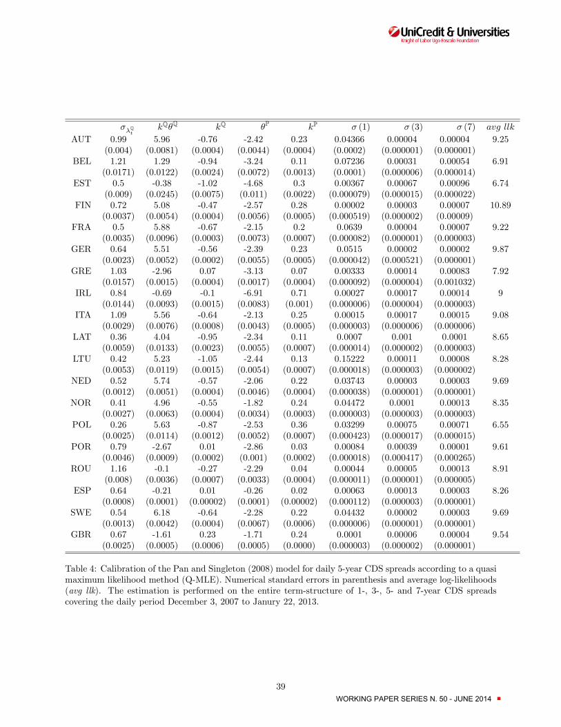
��QtkQ�Q kQ �P kP � (1) � (3) � (7) avg llk

AUT 0.99 5.96 -0.76 -2.42 0.23 0.04366 0.00004 0.00004 9.25(0.004) (0.0081) (0.0004) (0.0044) (0.0004) (0.0002) (0.000001) (0.000001)

BEL 1.21 1.29 -0.94 -3.24 0.11 0.07236 0.00031 0.00054 6.91(0.0171) (0.0122) (0.0024) (0.0072) (0.0013) (0.0001) (0.000006) (0.000014)

EST 0.5 -0.38 -1.02 -4.68 0.3 0.00367 0.00067 0.00096 6.74(0.009) (0.0245) (0.0075) (0.011) (0.0022) (0.000079) (0.000015) (0.000022)

FIN 0.72 5.08 -0.47 -2.57 0.28 0.00002 0.00003 0.00007 10.89(0.0037) (0.0054) (0.0004) (0.0056) (0.0005) (0.000519) (0.000002) (0.00009)

FRA 0.5 5.88 -0.67 -2.15 0.2 0.0639 0.00004 0.00007 9.22(0.0035) (0.0096) (0.0003) (0.0073) (0.0007) (0.000082) (0.000001) (0.000003)

GER 0.64 5.51 -0.56 -2.39 0.23 0.0515 0.00002 0.00002 9.87(0.0023) (0.0052) (0.0002) (0.0055) (0.0005) (0.000042) (0.000521) (0.000001)

GRE 1.03 -2.96 0.07 -3.13 0.07 0.00333 0.00014 0.00083 7.92(0.0157) (0.0015) (0.0004) (0.0017) (0.0004) (0.000092) (0.000004) (0.001032)

IRL 0.84 -0.69 -0.1 -6.91 0.71 0.00027 0.00017 0.00014 9(0.0144) (0.0093) (0.0015) (0.0083) (0.001) (0.000006) (0.000004) (0.000003)

ITA 1.09 5.56 -0.64 -2.13 0.25 0.00015 0.00017 0.00015 9.08(0.0029) (0.0076) (0.0008) (0.0043) (0.0005) (0.000003) (0.000006) (0.000006)

LAT 0.36 4.04 -0.95 -2.34 0.11 0.0007 0.001 0.0001 8.65(0.0059) (0.0133) (0.0023) (0.0055) (0.0007) (0.000014) (0.000002) (0.000003)

LTU 0.42 5.23 -1.05 -2.44 0.13 0.15222 0.00011 0.00008 8.28(0.0053) (0.0119) (0.0015) (0.0054) (0.0007) (0.000018) (0.000003) (0.000002)

NED 0.52 5.74 -0.57 -2.06 0.22 0.03743 0.00003 0.00003 9.69(0.0012) (0.0051) (0.0004) (0.0046) (0.0004) (0.000038) (0.000001) (0.000001)

NOR 0.41 4.96 -0.55 -1.82 0.24 0.04472 0.0001 0.00013 8.35(0.0027) (0.0063) (0.0004) (0.0034) (0.0003) (0.000003) (0.000003) (0.000003)

POL 0.26 5.63 -0.87 -2.53 0.36 0.03299 0.00075 0.00071 6.55(0.0025) (0.0114) (0.0012) (0.0052) (0.0007) (0.000423) (0.000017) (0.000015)

POR 0.79 -2.67 0.01 -2.86 0.03 0.00084 0.00039 0.00001 9.61(0.0046) (0.0009) (0.0002) (0.001) (0.0002) (0.000018) (0.000417) (0.000265)

ROU 1.16 -0.1 -0.27 -2.29 0.04 0.00044 0.00005 0.00013 8.91(0.008) (0.0036) (0.0007) (0.0033) (0.0004) (0.000011) (0.000001) (0.000005)

ESP 0.64 -0.21 0.01 -0.26 0.02 0.00063 0.00013 0.00003 8.26(0.0008) (0.0001) (0.00002) (0.0001) (0.00002) (0.000112) (0.000003) (0.000001)

SWE 0.54 6.18 -0.64 -2.28 0.22 0.04432 0.00002 0.00003 9.69(0.0013) (0.0042) (0.0004) (0.0067) (0.0006) (0.000006) (0.000001) (0.000001)

GBR 0.67 -1.61 0.23 -1.71 0.24 0.0001 0.00006 0.00004 9.54(0.0025) (0.0005) (0.0006) (0.0005) (0.0000) (0.000003) (0.000002) (0.000001)

Table 4: Calibration of the Pan and Singleton (2008) model for daily 5-year CDS spreads according to a quasimaximum likelihood method (Q-MLE). Numerical standard errors in parenthesis and average log-likelihoods(avg llk). The estimation is performed on the entire term-structure of 1-, 3-, 5- and 7-year CDS spreadscovering the daily period December 3, 2007 to Janury 22, 2013.


Panel A Panel BCredit Risk Premium Default Risk Credit Risk Premium (%)

Mean Std Dev Median Mean Std Dev Median Mean Std Dev Median34.1 22.8 32.1 37.5 23.5 36.1 Austria 47.1 1.0 47.041.5 28.4 35.9 53.5 37.2 46.2 Belgium 44.2 1.3 43.866.1 49.5 45.6 112.8 103.0 69.2 Estonia 38.9 2.5 39.618.4 11.8 15.2 17.4 10.1 15.0 Finland 50.4 1.9 50.628.3 17.8 25.9 30.7 20.3 27.4 France 48.6 1.1 48.510.6 6.4 9.7 21.7 11.3 21.1 Germany 31.6 2.1 31.6257.3 577.8 55.0 1142.1 2193.5 236.6 Greece 19.0 1.5 18.9303.3 251.4 196.2 32.4 16.3 27.7 Ireland 83.9 11.7 87.660.4 46.3 45.9 112.5 75.1 91.0 Italy 33.0 3.1 33.5110.5 68.0 83.2 253.7 158.0 186.6 Latvia 30.4 1.4 30.3103.7 53.6 91.8 171.9 99.5 147.1 Lithuania 38.3 1.5 38.48.5 9.7 4.8 34.5 17.8 32.3 Netherlands 14.4 9.0 12.813.0 7.2 11.1 8.0 4.3 6.9 Norway 61.5 0.6 61.765.0 32.6 59.5 80.7 38.6 75.0 Poland 44.3 1.0 44.499.7 93.3 75.1 289.5 293.8 201.5 Portugal 28.8 3.9 27.3125.5 49.4 116.0 179.1 82.1 161.2 Romania 41.7 1.3 41.868.5 44.2 63.8 107.6 69.9 101.6 Spain 39.1 0.7 39.019.3 13.4 17.9 20.6 15.5 18.6 Sweden 49.4 1.6 49.20.3 0.2 0.3 29.2 14.3 30.3 UK 53.2 0.5 53.275.5 72.8 51.8 144.0 172.9 80.6 mean 42.0 2.5 42.0

Table 5: Descriptive statistics of the two components (Panel A) embedded in the 5-year CDS spreads. Theestimation is performed on a daily basis with the Q-MLE method over the period December 3, 2007 toJanuary 22, 2013. The data are in basis points. Panel B reports the Credit Risk Premia as a percentage ofthe observed 5-year CDS spread.


(1) (2) (3) (4) (5) (6) (7)� lnCRPt � lnCRPt � lnCRPt � lnCRPt � lnCRPt � lnCRPt � lnCRPt

� lnPolIdxt 0.740*** 0.432** 0.320* 0.304* 0.279 0.513*** 0.452**[3.65] [2.48] [1.77] [1.71] [1.58] [2.77] [2.38]

� lnPolIdxt�1 0.791*** 0.367** 0.321* 0.320* 0.336* 0.268 0.318*[3.79] [2.38] [1.93] [1.91] [2.00] [1.47] [1.84]

� lnStockt -1.241*** -0.950*** -0.939*** -0.946*** -0.504**[-5.50] [-3.64] [-3.70] [-3.69] [-2.15]

� lnV 2Xt 0.0843 -0.0115 -0.0131 -0.00679 0.265[0.91] [-0.12] [-0.13] [-0.07] [1.57]

� ln iT raxxt 0.437*** 0.415** 0.399** 0.317[2.75] [2.55] [2.47] [0.95]

� lnPEEuro50t -0.0882[-0.84]

� lnPEDaxt -0.151*** -0.119***[-2.72] [-3.08]

� lnMSCIt -1.453*** -1.132***[-5.79] [-4.22]

� lnV IXt -0.201 -0.477**[-1.50] [-2.29]

� ln IGCDXt 0.246 -0.0981[1.60] [-0.28]

� lnTEDt 0.0663 0.0401[1.07] [0.64]

� lnGoldt 0.247 0.369[0.82] [1.19]

cons 0.005 0.0006 0.0002 0.0009 0.0007 -0.002 -0.009[0.16] [0.02] [0.01] [0.04] [0.03] [-0.09] [-0.37]

N 1129 1129 1129 1129 1129 1129 1129R2 0.193 0.307 0.350 0.352 0.361 0.379 0.408

Table 6: Credit Risk Premium: Panel regressions of CRP on the policy-related uncertainty index (PolIdx), thedomestic stock markets (Stock), the Eurostoxx50 and S&P500 implied volatility (V2X and VIX), the iTraxxEuro CDX and IG US CDX (iTraxx and IGCDX), the price-earning ratio of Eurostoxx50 and Dax Indices(PEdax and PEEuro50), the MSCI Global Equity Index (MSCI), the TED spread (TED) and the gold price(Gold). Tha variables are in log-di¤erences. Country �xed e¤ect included. Monthly sample period December3, 2007 to January 22, 2013. t-Stats in brackets, and errors clustered across time. Level of signi�cance: 1***,5** and 10* per cent.


(1) (2) (3) (4) (5) (6) (7)� lnDRPt � lnDRPt � lnDRPt � lnDRPt � lnDRPt � lnDRPt � lnDRPt

� lnPolIdxt 0.682*** 0.418*** 0.307* 0.291* 0.268* 0.465*** 0.404**[3.79] [2.75] [1.95] [1.90] [1.76] [3.01] [2.48]

� lnPolIdxt�1 0.730*** 0.355** 0.310** 0.309* 0.324** 0.253 0.294*[3.99] [2.51] [2.01] [1.98] [2.07] [1.54] [1.83]

� lnStockt -1.130*** -0.844*** -0.833*** -0.840*** -0.428**[-5.73] [-3.99] [-4.09] [-4.08] [-2.66]

� lnV 2Xt 0.0610 -0.0335 -0.0351 -0.0289 0.167[0.75] [-0.39] [-0.40] [-0.33] [1.13]

� ln iT raxxt 0.431*** 0.409*** 0.394*** 0.300[3.06] [2.83] [2.76] [0.99]

� lnPEEuro50t -0.0870[-0.87]

� lnPEDaxt -0.146*** -0.117***[-2.83] [-3.44]

� lnMSCIt -1.280*** -1.002***[-5.59] [-4.26]

� lnV IXt -0.184 -0.360**[-1.63] [-2.04]

� ln IGCDXt 0.260* -0.0676[1.92] [-0.21]

� lnTEDt 0.0631 0.0362[1.13] [0.62]

� lnGoldt 0.229 0.327[0.87] [1.19]

cons 0.005 0.0007 0.0002 0.001 0.0007 -0.001 -0.007[0.16] [0.03] [0.01] [0.04] [0.03] [-0.05] [-0.29]

N 1129 1129 1129 1129 1129 1129 1129R2 0.227 0.351 0.408 0.411 0.422 0.442 0.469

Table 7: Default Risk: Panel regressions of DRP on the policy-related uncertainty index (PolIdx), the domesticstock markets (Stock), the Eurostoxx50 and S&P500 implied volatility (V2X and VIX), the iTraxx Euro CDXand IG US CDX (iTraxx and IGCDX), the price-earning ratio of Eurostoxx50 and Dax Indices (PEdax andPEEuro50), the MSCI Global Equity Index (MSCI), the TED spread (TED) and the gold price (Gold). Thavariables are in log-di¤erences. Country �xed e¤ect included. Monthly sample period December 3, 2007 toJanuary 22, 2013. t-Stats in brackets and errors clustered across time. Level of signi�cance: 1***, 5** and10* per cent.


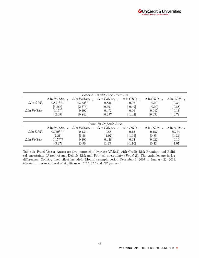
Panel A: Credit Risk Premium� lnPolIdxt�1 � lnPolIdxt�2 � lnPolIdxt�3 � lnCRPt�1 � lnCRPt�2 � lnCRPt�3

� lnCRPt 0.827*** 0.752** 0.836 -0.06 -0.00 -0.34[5.865] [2.375] [0.691] [-0.49] [-0.00] [-0.88]

� lnPolIdxt -0.15** 0.102 0.472 -0.06 0.047 -0.11[-2.49] [0.843] [0.997] [-1.42] [0.933] [-0.78]

Panel B : Default Risk� lnPolIdxt�1 � lnPolIdxt�2 � lnPolIdxt�3 � lnDRPt�1 � lnDRPt�2 � lnDRPt�3

� lnDRPt 0.759*** 0.433 -0.88 -0.13 0.157 0.274[7.21] [1.56] [-1.07] [-1.05] [0.85] [1.23]

� lnPolIdxt -0.17*** 0.100 0.446 -0.04 0.022 -0.10[-3.27] [0.99] [1.33] [-1.10] [0.42] [-1.07]

Table 8: Panel Vector Autoregressive approach: bivariate VAR(3) with Credit Risk Premium and Politi-cal uncertainty (Panel A) and Default Risk and Political uncertainty (Panel B). Tha variables are in log-di¤erences. Country �xed e¤ect included. Monthly sample period December 3, 2007 to January 22, 2013.t-Stats in brackets. Level of signi�cance: 1***, 5** and 10* per cent.


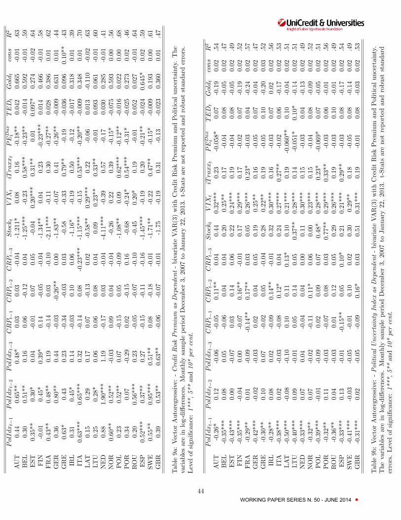
PolIdxt�1

PolIdxt�2

PolIdxt�3

CRPt�1

CRPt�2

CRPt�3

Stockt

VIXt

iTraxxt

PEDax

tTEDt

Goldt

cons

R2

AUT

0.44

0.65**

0.48*

0.03

0.03

-0.04

-1.211*

0.08

0.16

-0.18**

0.042

0.665

-0.01

.63

BEL

0.30

0.51**

0.16

0.06

-0.12

0.04

-1.25***

-0.23

0.58***

-0.23**

-0.014

0.592

-0.01

.59

EST

0.35**

0.30*

0.04

-0.01

0.07

0.05

-0.04

0.20***

0.31**

0.01

0.097*

0.274

-0.02

.64

FIN

-0.01

0.45*

0.39*

0.14

-0.05

-0.04

-1.34**

0.04

0.23

-0.23***

0.014

0.466

-0.01

.58

FRA

0.43**

0.48**

0.19

-0.14

0.03

-0.10

-2.11***

-0.11

0.30

-0.27**

0.028

0.386

0.01

.62

GER

0.36

0.80**

0.44

-0.03

-0.26**

0.00

-1.83**

-0.07

0.41

-0.26**

-0.009

0.631

0.01

.44

GRE

0.63*

0.43

0.23

-0.34

-0.03

0.03

-0.58

-0.33

0.79**

-0.19

-0.036

0.096

0.10**

.43

IRL

0.31

0.45*

0.14

-0.03

0.10

0.06

-1.16*

-0.19

0.50

-0.12

-0.017

0.318

0.01

.39

ITA

0.63***

0.65***

0.32

-0.14

0.08

-0.23***

-1.15***

-0.15

0.53***

-0.20**

-0.009

0.348

0.01

.70

LAT

0.15

0.29

0.17

0.07

-0.13

0.02

-0.58**

0.29***

0.22

-0.06

0.013

-0.110

-0.02

.63

LTU

0.25

0.28*

0.06

0.06

0.08

0.04

0.09

0.23**

0.33**

-0.01

0.093

0.061

-0.01

.60

NED

0.88

1.90***

1.19

-0.17

0.03

-0.04

-4.11***

-0.39

0.57

-0.17

0.030

0.285

-0.01

.41

NOR

0.60**

0.52**

-0.03

0.09

0.04

-0.04

-0.26

0.22

0.39

-0.15*

-0.075

0.593

0.00

.56

POL

0.23

0.52**

0.07

-0.15

0.05

-0.09

-1.08**

0.09

0.62***

-0.12**

-0.016

0.022

0.00

.68

POR

0.34

0.07

-0.29

0.02

-0.15

0.16

-0.68

-0.24*

0.54***

-0.31*

-0.025

0.273

0.02

.46

ROU

0.20

0.56***

0.23

-0.05

-0.07

-0.10

-0.45

0.20*

0.19

-0.01

0.052

0.027

-0.01

.64

ESP

0.52***

0.37**

0.27

-0.15

-0.11

-0.16

-1.45***

-0.19

0.20

-0.21**

-0.024

0.645*

0.02

.59

SWE

0.55**

0.95***

0.51**

0.08

-0.18

-0.01

-1.71**

-0.22

0.47**

-0.15*

-0.009

0.193

0.00

.61

GBR

0.39

0.53**

0.63**

-0.06

-0.07

-0.01

-1.75

-0.19

0.31

-0.13

-0.023

0.360

0.01

.47

Table9a:VectorAutoregressive:-CreditRiskPremiumasDependent-bivariateVAR(3)withCreditRiskPremiumandPoliticaluncertainty.The

variablesareinlog-di¤erences.MonthlysampleperiodDecember3,2007toJanuary22,2013.t-Statsarenotreportedandrobuststandarderrors.

Levelofsigni�cance:1***,5**and10*percent.

PolIdxt�1

PolIdxt�2

PolIdxt�3

CRPt�1

CRPt�2

CRPt�3

Stockt

VIXt

iTraxxt

PEDax

tTEDt

Goldt

cons

R2

AUT

-0.26*

0.12

-0.06

-0.05

0.11**

0.04

0.44

0.32***

0.23

-0.058*

0.07

-0.19

0.02

.54

BEL

-0.35***

0.08

0.05

-0.06

0.04

0.04

0.20

0.25**

0.17

-0.04

0.08

-0.05

0.02

.47

EST

-0.43***

0.00

-0.07

0.03

0.14

0.06

0.22

0.24***

0.19

-0.04

0.08

-0.05

0.02

.49

FIN

-0.35***

-0.04

0.00

-0.07

0.16**

-0.01

0.17

0.29***

0.17

-0.02

0.07

-0.19

0.02

.52

FRA

-0.29**

0.01

-0.09

-0.14**

0.17**

0.03

0.05

0.26***

0.23*

-0.03

0.04

-0.24

0.02

.57

GER

-0.42***

-0.02

-0.03

0.02

0.04

0.05

0.19

0.25**

0.16

-0.05

0.07

-0.04

0.02

.47

GRE

-0.30**

0.10

0.07

-0.02

0.05

-0.04

0.28

0.22**

0.19

-0.05

0.10

-0.20

0.03

.52

IRL

-0.28**

0.08

0.02

-0.09

0.14**

-0.01

0.32

0.30***

0.16

-0.03

0.07

0.02

0.02

.56

ITA

-0.38***

0.02

-0.03

-0.08

0.12*

0.04

0.24

0.27***

0.27**

-0.02

0.06

-0.17

0.02

.53

LAT

-0.50***

-0.08

-0.10

0.10

0.11

0.13*

0.10

0.21***

0.19

-0.060**

0.10

-0.04

0.02

.51

LTU

-0.40***

0.09

-0.01

0.05

0.14

0.05

0.37**

0.28***

0.14

-0.051*

0.10*

-0.14

0.02

.51

NED

-0.33***

0.07

0.04

-0.04

0.04

0.00

0.11

0.30***

0.15

-0.03

0.04

-0.13

0.02

.49

NOR

-0.32**

0.07

-0.02

-0.11

0.11*

0.06

0.00

0.23***

0.15

-0.04

0.08

-0.09

0.02

.52

POL

-0.39***

-0.01

-0.09

0.02

0.09

0.07

0.48*

0.28***

0.23*

-0.069*

0.07

-0.05

0.02

.51

POR

-0.32**

0.11

-0.03

-0.07

0.08

0.03

0.77**

0.29***

0.33**

-0.03

0.06

-0.01

0.02

.56

ROU

-0.36**

0.04

-0.03

0.01

0.12

0.05

0.29

0.26***

0.19

-0.03

0.10

-0.01

0.02

.49

ESP

-0.33***

0.13

-0.01

-0.15**

0.05

0.10*

0.21

0.21***

0.29**

-0.03

0.08

-0.17

0.02

.54

SWE

-0.41***

-0.03

-0.05

-0.01

0.10

0.02

0.30

0.29**

0.18

-0.05

0.08

-0.14

0.02

.49

GBR

-0.31***

0.02

-0.05

-0.09

0.16*

0.03

0.51

0.31***

0.19

-0.01

0.08

-0.03

0.02

.53

Table9b:VectorAutoregressive:-PoliticalUncertaintyIndexasDependent-bivariateVAR(3)withCreditRiskPremiumandPoliticaluncertainty.

Thevariablesareinlog-di¤erences.MonthlysampleperiodDecember3,2007toJanuary22,2013.t-Statsarenotreportedandrobuststandard

errors.Levelofsigni�cance:1***,5**and10*percent.


PolIdxt�1

PolIdxt�2

PolIdxt�3

DRPt�1

DRPt�2

DRPt�3

Stockt

VIXt

iTraxxt

PEDax

tTEDt

Goldt

cons

R2

AUT

0.52*

0.70**

0.42

0.05

0.05

-0.07

-1.13**

0.17

0.02

-0.15**

0.08

0.56

-0.01

.62

BEL

0.36

0.53**

0.15

0.04

-0.11

0.03

-0.92**

-0.16

0.45*

-0.26***

0.06

0.76

-0.01

.56

EST

0.33

0.34

0.08

-0.14

0.11

-0.01

-0.83

0.14

0.12

0.05

0.17**

0.29

-0.03

.64

FIN

-0.10

0.28

0.42**

0.14

-0.02

-0.11

-1.14***

0.07

0.07

-0.17***

0.10

0.29

0.00

.57

FRA

0.41

0.35

0.12

-0.11

0.04

-0.08

-1.10***

0.09

0.33

-0.28**

0.05

0.51

0.02

.58

GER

0.35

0.59

0.33

-0.01

-0.19

-0.04

-0.76

0.14

0.25

-0.25**

-0.01

0.44

0.00

.40

GRE

0.64

0.54

0.29

-0.36*

-0.09

0.00

-0.74

-0.43

0.79*

-0.23

0.03

0.11

0.13***

.44

IRL

0.07

0.15

0.00

-0.07

0.18

0.01

-0.69**

-0.12

0.13

-0.02

0.02

0.20

0.00

.33

ITA

0.42**

0.52***

0.26

-0.12

0.04

-0.20***

-0.76**

-0.13

0.52***

-0.18**

0.01

0.31

0.02

.64

LAT

0.15

0.23

0.09

0.15

-0.05

0.04

-0.69*

0.15

0.07

-0.05

0.06

-0.30

-0.02

.62

LTU

0.15

0.19

0.06

-0.06

0.13

-0.04

-0.81*

0.16

0.14

0.02

0.145*

0.08

-0.01

.61

NED

0.49

0.46

0.29

-0.10

0.01

-0.03

-0.63

0.05

0.54*

-0.08

-0.05

0.64

0.00

.49

NOR

0.51**

0.43*

-0.01

0.02

0.10

-0.10

-0.87*

0.15

0.19

-0.11

-0.02

0.56

-0.01

.59

POL

0.20

0.50**

0.02

-0.18

0.06

-0.08

-0.94**

0.08

0.45**

-0.12**

0.02

0.02

-0.01

.65

POR

0.33

0.04

-0.36

-0.01

-0.19

0.16

-0.80

-0.35*

0.59**

-0.40**

0.01

0.37

0.03

.47

ROU

0.17

0.64***

0.24

-0.09

-0.03

-0.11

-0.92*

0.17

0.04

0.02

0.15

0.09

-0.01

.63

ESP

0.43*

0.27

0.12

-0.13

-0.16

-0.13

-0.81*

-0.16

0.36*

-0.24*

-0.01

0.48

0.03

.51

SWE

0.58*

0.76**

0.49*

0.12

-0.17

-0.08

-1.18***

-0.07

0.24

-0.18*

0.05

0.09

-0.01

.59

GBR

0.23

0.31

0.616**

-0.10

-0.03

-0.11

-1.48**

-0.10

0.00

-0.07

0.10

0.28

0.01

.51

Table10a:VectorAutoregressive:-DefaultRiskasDependent-bivariateVAR(3)withDefaultRiskandPoliticaluncertainty.Thevariablesare

inlog-di¤erences.MonthlysampleperiodDecember3,2007toJanuary22,2013.t-Statsarenotreportedandrobuststandarderrors.Levelof

signi�cance:1***,5**and10*percent.

PolIdxt�1

PolIdxt�2

PolIdxt�3

DRPt�1

DRPt�2

DRPt�3

Stockt

VIXt

iTraxxt

PEDax

tTEDt

Goldt

cons

R2

AUT

-0.26**

0.10

-0.06

-0.06

0.11**

0.067*

0.56**

0.31***

0.30**

-0.074*

0.05

-0.19

0.02

.57

BEL

-0.29**

0.13

0.04

-0.03

0.02

0.06

0.47*

0.28***

0.26*

-0.05

0.05

-0.07

0.02

.51

EST

-0.32***

0.04

-0.08

0.05

0.05

0.12**

0.66**

0.29***

0.34**

-0.085*

0.04

-0.05

0.02

.53

FIN

-0.29**

0.03

-0.03

-0.05

0.153*

0.04

0.48*

0.32***

0.26**

-0.04

0.05

-0.15

0.02

.55

FRA

-0.23*

0.07

-0.08

-0.12**

0.14**

0.04

0.33

0.29***

0.29**

-0.04

0.03

-0.22

0.02

.59

GER

-0.32**

0.06

-0.04

0.03

0.03

0.085*

0.56**

0.29***

0.28**

-0.068*

0.04

0.00

0.02

.52

GRE

-0.27*

0.11

0.04

-0.03

0.05

-0.02

0.41

0.27***

0.22

-0.05

0.07

-0.17

0.02

.52

IRL

-0.29**

0.11

0.06

-0.15

0.18*

0.01

0.34

0.28***

0.20*

-0.05

0.06

-0.04

0.02

.53

ITA

-0.29**

0.08

-0.04

-0.09

0.15*

0.07

0.50**

0.31***

0.33**

-0.03

0.04

-0.18

0.02

.56

LAT

-0.34***

-0.02

-0.09

0.17*

0.02

0.21**

0.75**

0.30***

0.36**

-0.098***

0.06

-0.12

0.026*

.58

LTU

-0.32**

0.05

-0.05

0.05

0.04

0.11

0.62**

0.29***

0.32**

-0.07**

0.05

-0.06

0.02

.52

NED

-0.25*

0.10

-0.09

-0.03

0.08

0.11**

0.59**

0.31***

0.31**

-0.07

0.03

-0.02

0.02

.56

NOR

-0.28**

0.11

-0.03

-0.08

0.10

0.08

0.38

0.28***

0.24**

-0.06

0.06

-0.10

0.02

.54

POL

-0.34**

0.03

-0.07

0.03

0.07

0.09

0.58**

0.29***

0.31**

-0.074*

0.05

-0.05

0.02

.53

POR

-0.31***

0.11

0.02

-0.07

0.08

0.02

0.37

0.29***

0.23*

-0.03

0.05

-0.04

0.02

.52

ROU

-0.30**

0.08

-0.02

0.01

0.06

0.07

0.55**

0.29***

0.28**

-0.06

0.06

-0.05

0.02

.51

ESP

-0.28**

0.17

0.02

-0.13**

0.04

0.10**

0.36

0.23***

0.31**

-0.04

0.07

-0.13

0.02

.56

SWE

-0.31**

0.07

-0.07

0.00

0.09

0.075**

0.68**

0.33***

0.34**

-0.06

0.05

-0.16

0.02

.55

GBR

-0.26**

0.09

-0.04

-0.07

0.14

0.06

0.49

0.29***

0.29**

-0.03

0.05

-0.02

0.02

.56

Table10b:VectorAutoregressive:-PoliticalUncertaintyIndexasDependent-bivariateVAR(3)withDefaultRiskandPoliticaluncertainty.The

variablesareinlog-di¤erences.MonthlysampleperiodDecember3,2007toJanuary22,2013.t-Statsarenotreportedandrobuststandarderrors.

Levelofsigni�cance:1***,5**and10*percent.


Core Economies Peripheral Economies Eastern Economies(1a) (1b) (2a) (2b) (3a) (3b)

CRPCoret PolIdxt CRPPeripht PolIdxt CRPEastt PolIdxtCRPCoret�1 0.260*** -0.101CRPCoret�2 -0.101 0.171***CRPCoret�3 -0.0152 0.0532

CRPPeripht�1 -0.194** -0.119*CRPPeripht�2 0.0002 0.0627CRPPeripht�3 -0.0429 0.0692CRPEastt�1 -0.108 0.0860CRPEastt�2 -0.0681 0.0712CRPEastt�3 -0.0723 0.0915PolIdxt�1 -0.200 -0.357*** 0.352** -0.342*** 0.0692 -0.456***PolIdxt�2 0.0631 -0.0227 0.0349 0.0591 0.272** -0.0425PolIdxt�3 0.163 -0.112 -0.0986 -0.0320 0.194 -0.0974CRPCoret 0.627*** 0.136 0.436*** 0.0593

CRPPeripht 0.524*** 0.134* 0.0146 0.150CRPEastt 0.505*** 0.109 0.00852 0.112

Daxt -0.800* -0.570 1.601*** -0.155 -0.349 -0.438MSCIt 0.320 0.767*** -0.990*** 0.666** -0.340 0.950***V 2Xt 0.0869 -0.161 0.228 -0.144 -0.0193 -0.168

iT raxxt -0.266 0.483** 0.220 0.396** 0.132 0.365*PEDaxt -0.159** -0.00994 -0.0783 -0.00524 0.157** -0.0204V IXt -0.0640 0.432*** -0.348** 0.382*** 0.0876 0.457***

IGCDXt 0.190 -0.373* 0.101 -0.217 -0.176 -0.183TEDt 0.0144 0.0244 -0.00498 0.0295 0.0796 0.0300Goldt 0.222 -0.284 0.217 -0.173 0.0766 -0.135cons -0.00140 0.0183* 0.0221 0.0188 -0.0207* 0.0203*

N 58 58 58 58 58 58R2 0.865 0.645 0.776 0.585 0.774 0.578

Table 11: Vector Autoregressive approach on region level: bivariate VAR(3) with Credit Risk Premium andPolitical uncertainty. Variables: the policy-related uncertainty index (PolIdx), the domestic stock markets(Stock), the Eurostoxx50 and S&P500 implied volatility (V2X and VIX), the iTraxx Euro CDX and IG USCDX (iTraxx and IGCDX), the price-earning ratio of Eurostoxx50 and Dax Indices (PEdax and PEEuro50),the MSCI Global Equity Index (MSCI), the TED spread (TED) and the gold price (Gold). The variablesare in log-di¤erences. Core Economies are Austria, Finland, France, Germany, Netherlands, Norway, Swedenand UK; Peripheral Economies are Belgium, Greece, Ireland, Italy, Portugal and Spain; Eastern Economiesare Estonia, Latvia, Lithuania, Poland and Romania. Monthly sample period December 3, 2007 to January22, 2013. t-Stats are not reported and robust standard errors. Level of signi�cance: 1***, 5** and 10* percent.


Core Economies Peripheral Economies Eastern Economies(1a) (1b) (2a) (2b) (3a) (3b)

DRPCoret PolIdxt DRPPeripht PolIdxt DRPEastt PolIdxtDRPCoret�1 0.142 -0.0323DRPCoret�2 -0.188** 0.0968*DRPCoret�3 0.0282 0.0836*

DRPPeripht�1 -0.211** -0.178***DRPPeripht�2 -0.0644 0.0745DRPPeripht�3 -0.148** 0.0922*DRPEastt�1 -0.0666 0.0871DRPEastt�2 0.104 0.0457DRPEastt�3 -0.0515 0.109*PolIdxt�1 0.0407 -0.387*** 0.329** -0.349*** -0.0679 -0.448***PolIdxt�2 0.186 0.0483 0.147 0.124 0.0578 -0.0214PolIdxt�3 0.504*** -0.0943 -0.0664 -0.0801 -0.0150 -0.0759DRPCoret 0.380*** 0.0847 0.294*** -0.00158

DRPPeripht 0.600*** 0.135 0.178 0.198**DRPEastt 0.454*** 0.0381 0.254** 0.0617

Daxt -0.141 -0.452 -0.211 -0.563 -0.140 -0.388MSCIt 0.0562 0.817*** -0.439 0.578** -0.431 0.939***V 2Xt 0.274 -0.128 0.133 -0.156 -0.180 -0.143

iT raxxt -0.523 0.425** 0.689*** 0.600*** 0.00790 0.325PEDaxt -0.0725 -0.00714 -0.202*** -0.0164 0.131* -0.0231V IXt -0.278 0.395*** -0.368** 0.323** 0.357** 0.417***

IGCDXt 0.493 -0.217 -0.620** -0.376* -0.0213 -0.0927TEDt 0.0250 0.0313 -0.0565 0.0369 0.132** 0.0412Goldt 0.111 -0.159 0.433* -0.162 -0.193 -0.147cons 0.00135 0.0171 0.0229 0.0174 -0.0158 0.0198*

N 58 58 58 58 58 58R2 0.78 0.6 0.76 0.61 0.74 0.57

Table 12: Vector Autoregressive approach on region level: bivariate VAR(3) with Default Risk and Politicaluncertainty. Variables: the policy-related uncertainty index (PolIdx), the domestic stock markets (Stock),the Eurostoxx50 and S&P500 implied volatility (V2X and VIX), the iTraxx Euro CDX and IG US CDX(iTraxx and IGCDX), the price-earning ratio of Eurostoxx50 and Dax Indices (PEdax and PEEuro50), theMSCI Global Equity Index (MSCI), the TED spread (TED) and the gold price (Gold). The variables are inlog-di¤erences. Core Economies are Austria, Finland, France, Germany, Netherlands, Norway, Sweden andUK; Peripheral Economies are Belgium, Greece, Ireland, Italy, Portugal and Spain; Eastern Economies areEstonia, Latvia, Lithuania, Poland and Romania. Monthly sample period December 3, 2007 to January 22,2013. t-Stats are not reported and robust standard errors. Level of signi�cance: 1***, 5** and 10* per cent.


What Moves the Systemic Credit Risk in Europe?

Gerardo Manzo�

PhD Candidate in Money and FinanceUniversity of Rome "Tor Vergata"

-Visiting Scholar Researcher

The University of Chicago Booth School of Business

August 2013

Abstract

I analyze the systemic nature of sovereign credit risk in the European Union. Exploiting a cross sectionof 24 countries and the Credit Default Swap term structures, I extract the systemic default intensity bycalibrating the Ang and Longta¤ (2011) sovereign CDS pricing model using the Unscented Kalman Filter.The systemic intensity reaches the highest peaks during the Lehman default and the Summer 2011 whenpolitical issues resounded in Europe. The empirical analysis shows how variations in the probability of asystemic breakdown are mostly driven by global stock and credit market variables. Moreover, I �nd thatpolitical uncertainty adds up a signi�cant amount of systemic credit risk, with a lead-lag e¤ect of onemonth. Finally, I �nd that higher default intensities in the European Union are associated with higherdebt over GDP and bank asset over GDP ratios. Such a linkage becomes positive and signi�cant whenthe European Commission started an important debate in 2010 about the �rst bailout in the EuropeanUnion history so far. Therefore, policy interventions aimed at reducing the large debts, at restoringgrowth rates and reaching a sort of political stability in the most developed European countries maycontribute signi�cantly to reduce the probability of a systemic breakdown of the whole European Union.

[JEL No. G12,G13,G18]Keywords: Systemic Credit Risk, Credit Default Swap, Political Uncertainty, Sovereign Debt, Eu-

ropean Union, Unscented Kalman Filter

�[email protected] .Gerardo Manzo is a PhD candidate in Money and Finance at the University of Rome "TorVergata". The paper was written while Gerardo Manzo was a visiting scholar at The University of Chicago Booth School ofBusiness.


Is the systemic nature of credit risk relevant for the European Union? What are its main driving forces?Are a large domestic banking system and a high degree of sovereign indebtness a signal of a high probabilityof a systemic breakdown? Does heterogeneity among European countries�economic systems matter in termsof credit risk? Does political uncertainty play a role in exacerbating the credit crisis?

I analyze these questions empirically, exploiting information embedded in the European sovereign creditmarket. The relevance of such questions is a result of the 2007/09 �nancial crisis. In fact, the �nancialcrisis, which began in mid-2007 with the crash of the US housing-bubble, has triggered a wave of sovereigndebt-increases in the Euro zone. Governments have run into debt in order to prevent the collapse of their own�nancial and banking systems. The growing amount of debt has resulted in a rapid widening of Europeancountries�credit spreads. Thus, di¢ culties in rolling-over the debt on capital markets have arisen, requiringthe intervention of third parties, such as the ECB, IMF and World Bank.

The increasing �nancial and economic linkages in both the European Union and the banking systemshave sparked a heated debate, among the European politicians, about the degree of interconnectedness of theeconomies which may exacerbate the propagation of common negative shocks. The high volatility experiencedin the European sovereign credit market has laid the basis for analyzing the systemic nature of credit risk.Therefore, in this work I enrich the understanding about the economic and �nancial forces that contributeto fuel the probability of a systemic breakdown of the European Union.

The literature that investigates the credit markets both empirically and theoretically has been growingsince the beginning of the �nancial crisis 2007/09. Indeed, investors have shifted their attention to thesovereign credit market because the wave of bailouts has made countries more �nancially constrained, hence,more prone to defaults. Pan and Singleton (2008) build a sovereign CDS pricing model which allows for thespread decomposition into a market price of risk and a default risk. They �nd that the market price of riskof some emerging markets, such as Turkey, Mexico and Korea, is statistically correlated with measures of�nancial market volatility (VIX), global event risk (US credit spread) and macroeconomic policy (currency-implied volatility). Longsta¤ et al. (2011) calibrate the same pricing model over a wider set of emergingmarkets and then regress the CDS spread components on local and global market variables, on di¤erentmeasures of risk premiums, such as equity, volatility and term premia and on global capital �ows. They �ndthat CDS-implied risk premia are more related to global economic measures than to local variables. Angand Longsta¤ (2011) modify the Pan and Singleton (2008) sovereign model including a systemic risk andcalibrating it cross-sectionally on two large geographic areas, Europe and the US. They �nd that the Eurozone shares a systemic credit risk greater than states in the US, and that credit risk is more a¤ected by�nancial markets than by macroeconomic fundamentals. Manzo (2012), following Pan and Singleton (2008),investigates the role of political uncertainty in the European sovereign credit market with a sample of 19countries. He �nds that political uncertainty a¤ects signi�cantly the credit risk premium in the Euro zone,namely, that premium asked by investors to bear the credit risk of that region on their portfolios.

Alongside empirical studies on the macro-determinants of credit spreads, theoretical works on the roleof political decisions in both stock and capital markets have recently been developed. Pastor and Veronesi(2012), Pastor and Veronesi (2011) and Ulrich (2011), among others. The former theoretically investigates thee¤ect of the government�s policy decision on the stock prices in a Bayesian-learning equilibrium framework.Their main result is that, on average, the stock price drops down, with this reduction being larger when theannouncement of a political change includes elements of surprise. Pastor and Veronesi (2011)�s model allowsfor the equity risk premium�s decomposition into three components related to three di¤erent shocks. Whilethe �rst two are deemed as economic shocks, the third one is the political shock which "a¤ect investors�beliefsabout which policy the government might adopt in the future". Moreover, using the Baker et al. (2011)�spolicy-related uncertainty index, they �nd empirical evidence that political uncertainty is state-dependent,since it is higher when worse economic conditions are in play. Lastly, Ulrich (2011) analyze the e¤ect ofpolitical uncertainty on the bond market through a pricing model that incorporates political uncertainty.The latter regards the Ricardian equivalence uncertainty (or Knightian uncertainty), according to whichinvestors expect a non-zero consumption growth rate after the implementation of a government policy. Themodel predicts that a government policy a¤ecting the business cycle leads to a positive risk premium forinvestors.

As outlined in Hansen (2012), the systemic risk has not to be confused with the systematic risk. In fact,the latter is concerned with "macroeconomic or aggregate risks that cannot be avoided through diversi�cation,[... and] investors, who are exposed to these risks, require compensation because there is no simple insurance


scheme whereby exposure to these risks can be averaged out."1 . Instead, the systemic risk stands for the risk ofa catastrophic breakdown of an entire macro region or �nancial market. Therefore, it requires policymakersto implement adequate measures of monitoring and intervention. Thus, understanding the main drivingfactors of the systemic risk may help out on this policy issue.

In particular, in the following work I exploit a cross section of 24 European countries, all members of theEuropean Union, to extract the systemic credit risk component which gives a measure of the vulnerability ofthe whole Europe. In fact, using a Credit Default Swap term structure for each country, I calibrate the Angand Longsta¤ (2011) pricing model to extract the intensity of default common to the entire cross section.Such an intensity gives a measure of the systemic probability of default over time. Unlike Ang and Longsta¤(2011), for the calibration I cast the model into a state space form by implementing the Unscented KalmanFilter (UKF). Such a �lter is known to give e¢ cient estimates of the states and is preferred when the systemof equations is non-linear.

Several �ndings emerge from this analysis: �rstly, sorting the entire cross section by their 2012-debtover GDP ratio, a clear pattern appears. The most indebted countries add up a certain risk which is thecombination not only of high indebtness which makes them more �nancially constrained, but also of negativereal growth rates and large banking systems that makes a bailout less likely; secondly, a Principal ComponentAnalysis performed on the correlation matrix of 5-year Credit Default Swap spreads shows that the �rst threePCs explain 80 per cent of the cross sectional variability during the �nancial crisis, which then becomes as lowas 60 per cent during the debt crisis. This di¤erence across the two subsamples signals that the heterogeneityof European countries in responding to shocks has increased during the debt crisis. Moreover, the Daxindex together with the volatility in the US market (VIX index) and the credit worthiness of the Europeanindustrial sector (iTraxx Euro CDX) explain alone almost the 32 per cent of the variability of the �rst PC�schanges; thirdly, calibrating the country-speci�c probability of default relative to that of Germany, I �ndthat the Eastern European countries contribute to the systemic credit risk as twice as Germany, whereasGreece, followed by Cyprus, concurs the most to increase the probability of a systemic breakdown with highcoe¢ cients of 7.56 and 3.67, respectively; fourthly, regressing the systemic default intensity on �nancial globalvariables, I �nd that both global and Europe-speci�c variables, such as the MSCI Global Financial Index, theVIX index, the iTraxx Euro CDX and the TED spread, explain almost the 40 per cent of the variability ofthe changes in the systemic probability of default of the European Union. In addition to this, I extend Manzo(2012) by investigating the role of policy-related uncertainty in the European credit market from a systemicpoint of view. I �nd that political uncertainty has a one-month lagged e¤ect on the systemic default intensitywith a standardized coe¢ cient of +14 per cent and with this e¤ect being robust to �nancial controls. Here thecontrols play a fundamental role, that is, they depurate the policy-related uncertainty index from �nancialvariations, leaving out only the political part as a residual. Moreover, Impulse Response Functions show howa political shock has an impact on the probability of a systemic breakdown which survives for three monthsbefore disappearing. Lastly, exploiting the cross section of the 24 European countries, I estimate the e¤ectof bank asset over GDP and public debt over GDP on the default intensities. Such an e¤ect is characterizedby an upward trend since the Lehman bankruptcy in September 2008, for then becoming signi�cant when,at the beginning of 2010, policy makers started an important debate about the �rst bailout in the EuropeanUnion history so far

The paper is organized as follows: Section 1 introduces the dataset used for the analysis; Section 2 presentsthe Ang and Longsta¤ (2011) pricing model and Section 3 its calibration techniques, that is, the UnscentedKalman Filter; Section 4 exposes the empirical analysis; Section 5 concludes the work.

1 Data

I use sovereign Credit Default Swap (CDS) spreads to capture the systemic risk implied in the Europeancredit market. When markets behave e¢ ciently, credit-sensitive securities do re�ect information about thecreditworthiness of a speci�c country. Indeed, CDS spreads provide a pure measure of the default risk sincethey are not a¤ected by maturity issues and callability options like sovereign bonds.

CDS spreads are collected from the Markit database and cover a period of 366 weeks from January 4,2006 to January 16, 2013 for the maturities 1-, 2-, 3-, 5- and 7-year and for 24 European countries. The latter

1Hansen, Peter Lars (2012), page 4.


are members of both the European Union and the Economic and Monetary Union. In particular, I considerAustria, Belgium, Cyprus, Estonia, Finland, France, Germany, Greece, Ireland, Italy, Malta, Netherlands,Portugal, Slovakia, Slovenia and Spain, as members of both the European Union and the Economic andMonetary Union. Then, Bulgaria, Czech Republic, Denmark, Latvia, Lithuania, Poland, Sweden and UnitedKingdom as members of only the European Union. The sample period and the number of countries aredictated by data availability. Thus, the total dataset consists of 43,920 weekly spreads aggregated by pickingup each Wednesday.

Figure 1 shows the average GDP real growth rate over the sample period and the banking asset over GDPratio for each country sorted by their level of indebtness with respect to the size of the economy. Since thebeginning of the �nancial crisis, the peripheral countries, such as Cyprus, Greece, Ireland, Italy, Portugal andSpain, have experienced negative real growth rates on average. This scenario may get worse when the bankingsystem is taken into account. Indeed, the bank assets over GDP ratio measures the ability of a country tosupport its own banking system in case of a breakdown. Thus, the combination of negative growth rates andlarge banking systems may signal a high risk of a systemic breakdown of the European Union. Indeed, highindebted countries in Europe have also large banking systems, so they can be deemed as strongly �nanciallyconstrained because they would not be able to support their own banking systems in case of a breakdown.

4

2

0

2

4

6

8

10

Estonia [10.1]

Bulgaria [18.5]

Sweden [38]

Lithuania [40.6]

Latvia [40.7]

Denmark [45.5]

Czech Rep [45.9]

Slovakia [52.1]

Finland [53.6]

Slovenia [54.1]

Poland [55.6]

Nether [71.3]

Malta [71.6]

Austria [73.2]

Germany [81.9]

Spain [84.2]

Cyprus [85.8]

UK [88.8]

France [90.2]

Belgium [99.8]

Ireland [117.4]

Portugal [123.7]

Italy [127]

Greece [156.9]

Estonia [10.1]

Bulgaria [18.5]

Sweden [38]

Lithuania [40.6]

Latvia [40.7]

Denmark [45.5]

Czech Rep [45.9]

Slovakia [52.1]

Finland [53.6]

Slovenia [54.1]

Poland [55.6]

Nether [71.3]

Malta [71.6]

Austria [73.2]

Germany [81.9]

Spain [84.2]

Cyprus [85.8]

UK [88.8]

France [90.2]

Belgium [99.8]

Ireland [117.4]

Portugal [123.7]

Italy [127]

Greece [156.9]

Low Debt/GDP Medium Debt/GDP High Debt/GDP

Real GDP GrowthBank Asset/GDP

Figure 1. The picture depicts the average real GDP growth rate and the bank asset over GDP ratio for theperiod Janury 2006 to January 2013. The square brackets report the debt over GDP ratio for the year 2012.

Credit Default Swap spreads clearly embed these default scenarios. Indeed, Table 1 reports summarystatistics of the 5-year CDS spreads for each country during both the 2007/09 �nancial crisis (Panel A) andthe 2010/13 European debt crisis (Panel B). The countries are sorted according to their debt over GDPratios as in 2012.

From the table it emerges that the Eastern Europe, namely, those countries characterized by low indebt-ness with respect to their economy, have experienced, on average, high spreads during the �nancial crisis.Indeed, domestic players of these economies leveraged themselves up with foreign-currency loans. When thecrisis burst, it brought about a wave of credit crunch that shocked the economies negatively. Therefore, whatmatters for these countries is the borrowing channel which can be problematic if the international creditsituation dries up. When the crisis turned up to be driven by the high indebtness of developed Europeancountries, the scenario reverted. Heavily indebted countries such as Greece, Cyprus, Ireland and Portugal arecharacterized by negative CDS term structure slopes during the European debt crisis, meaning that investorsexpect these countries not to be able to meet their obligations in the next future with a high probability. Infact, as a result of the large wave of banking systems�bailouts, the high indebtness of countries has increased


Panel A Panel BDebt/GDP Financial Crisis 2007/09 European Debt Crisis 2010/13in 2012 Mean Std Dev Slope Mean Std Dev Slope

Estonia 10.1 157.2 195.5 16.5 100.2 24.8 61.6Bulgaria 18.50 161.5 173.2 39.7 243.0 71.3 105.9Sweden 38.0 25.8 37.5 9.8 34.2 13.7 26.2

Low Lithuania 40.6 184.0 227.1 10.7 227.2 56.4 83.5Debt/GDP Latvia 40.7 271.7 318.1 2.3 263.5 92.1 71.1

Denmark 45.50 23.2 34.8 10.0 60.2 36.1 40.4Czech Rep 45.90 54.1 70.6 19.3 94.5 24.0 60.7Slovakia 52.1 46.7 54.4 19.0 130.0 68.7 72.2Finland 53.6 14.8 19.5 6.8 42.1 20.4 27.9Slovenia 54.1 38.2 49.3 16.4 183.3 124.6 80.2Poland 55.6 79.4 91.5 29.8 150.3 48.5 92.5

Medium Netherlands 71.3 20.1 29.7 7.1 47.5 21.5 30.6Debt/GDP Malta 71.6 40.2 43.6 19.6 254.0 103.1 36.1

Austria 73.20 36.0 55.0 11.3 75.3 33.3 44.9Germany 81.9 13.9 18.3 7.0 37.4 14.2 29.0Spain 84.2 37.2 41.3 17.5 251.2 86.5 56.5Cyprus 85.80 41.4 47.7 18.1 623.1 470.8 -96.4UK 88.8 29.5 40.6 12.8 67.7 16.2 50.1France 90.2 16.1 20.3 7.6 80.1 33.6 47.8

High Belgium 99.80 25.9 33.1 11.8 128.7 62.5 50.9Debt/GDP Ireland 117.4 64.6 90.9 13.8 485.2 249.2 -40.7

Portugal 123.7 35.4 35.6 17.6 614.7 358.2 -102.7Italy 127.0 46.9 50.5 21.7 236.6 116.2 60.6Greece 156.9 67.2 78.7 25.8 2866.9 4029.8 -2143.8

Table 1: The table reports summary statistics of 5-year Credit Default Swap spreads of 24 European countriesover the weekly period January 2006 to January 2013. Countries are sorted by their debt over GDP ratioas in 2012 and the statistics are shown across two subsamples: the 2007/09 �nancial crisis and the 2010/13European debt crisis.


signi�cantly the default risk of the whole European Union, with the peripheral economies su¤ering the mostnegative shocks. Such a scenario is clearly reported in Panel B of Table 1. As an example, during the �nancialcrisis, an investor would ask for a premium of 67.2 basis points to hedge against the default of Greece over a5-year horizon, which then increases as high as 2866.9 bps during the debt crisis. Such a high spread embedsan approximately risk-neutral probability of default of 31.8 per cent which became as high as 98 per cent theday before the selective default on March 8, 20122 . Conversely, the protection buyer would pay, on average,15 bps per year to hedge against a remote default of Germany. The whole picture that emerges from thissummary indicates that there is a consistent time variation in CDS spreads and heterogeneity in the waycountries react to negative shocks.

1.1 Commonality in the European Credit Market

In an environment of interconnected economies, such as the European Union, country-speci�c shocks can bepropagated to other economies leading to an increase in the probability of a breakdown of the whole Union.Such a systemic default probability may be priced in the credit market to the extent that it is moved by adefault intensity that is common across the European countries. In order to understand how much varianceof the CDS spreads is explained by the common components, I perform the Principal Component Analysison the correlation matrix of the �rst di¤erences in the 5-year CDS spreads. Results not reported here showthat the �rst three PCs explain the 80 per cent of the variability during the �nancial crisis, which thenbecomes as low as 60 per cent during the debt crisis. This di¤erence across the two subsamples signal thatthe heterogeneity of European countries in responding to shocks has increased during the debt crisis.

In order to investigate further the commonalities across the European Union, I perform the PCA on theweekly changes of CDS spreads scaled by the standard deviations to avoid that the magnitude of the Greekspread absorbes the entire variability. Figure 2 plots the loadings for the �rst three principal components.

0.1

0.2

0.3

Est

Bgr

Sw

eLt

uLv

aD

nkC

ze Svn Fin

Svk Pol

Nld Mlt

Aut

Deu

Esp

Cyp UK

Fra

Bel Irl Prt Ita Grc

1st P

C

Low Debt/GDP Medium Debt/GDP High Debt/GDP

0.2

0

0.2

Est

Bgr

Sw

eLt

uLv

aD

nkC

ze Svn Fin

Svk Pol

Nld Mlt

Aut

Deu

Esp

Cyp UK

Fra

Bel Irl Prt Ita Grc

2nd

PC

0.40.2

00.2

Est

Bgr

Sw

eLt

uLv

aD

nkC

ze Svn Fin

Svk Pol

Nld Mlt

Aut

Deu

Esp

Cyp UK

Fra

Bel Irl Prt Ita Grc

3rd

PC

Figure 2. Principal Components of weekly changes in 5-year CDS spreads.

The �rst PC presents positive loadings for the whole European Union. Thus, as Longsta¤ et al. (2011)point out, such a component re�ects "parallel shifts" in the cross section of the CDS spreads. Table 2panel A reports the pairwise correlations of the �rst three PCs with some interesting variables, that is, the

2The computation is simply performed under the assumption of a continuous payment of the premium, a constant intensityof default and a loss given default of 75 per cent. Under these assumptions, the intensity of default can be extracted by simplydividing the CDS spread by the loss given default. Moreover, they are risk-neutral probabilities.


Panel A: Correlation Structure� ln (Dax) � ln (SP500) � ln (V 2x) � ln (V ix) �CdxUS �CdxEU

1stPC -0.43 -0.40 0.32 0.27 0.47 0.562ndPC 0.21 0.29 -0.14 -0.18 -0.22 -0.173rdPC -0.17 -0.17 0.19 0.16 0.06 0.19

Panel B: Regression Analysiscons � ln (Dax) � ln (V ix) �CdxEU �CdxUS AdjR2 N

1stPC -0.00 -3.29*** -0.55** 0.030*** 0.00 0.32 365[-0.10] [-2.84] [-2.02] [5.38] [0.38]

2ndPC -0.00 1.37** -0.06 0.005* -0.007*** 0.06 365[-0.09] [2.14] [-0.40] [1.63] [-2.6]

3rdPC -0.00 -0.08 0.18 0.009*** -0.008*** 0.08 365[-0.08] [-0.1] [1.7] [4.4] [-4.0]

Table 2: The table reports the correlations of the �rst three principal components with �nancial variables(Panel A) and a regression analysis (Panel B). The PCs are extracted from weekly changes of CDS spreadsof 24 European countries over the period January 2006 to January 2013. Stock market variables are the Daxand SP500 indices. VIX and V2X are global market risk varibales for the US and the European market,respectively. CdxUS and CdxEU are the CDX IG 5y Corp and the ITraxx Eur CDSI 5y Corp. t-Stats inbrackets and robust standard errors. Level of signi�cance: 1***, 5** and 10* per cent

German stock market (Dax), the US stock market (S&P500), the US and European volatility (VIX andV2X, respectively) and the US and European iTraxx indices (CDX US and CDX EU, respectively) whichare proxies for the credit worthiness of the US and European industrial sector. All these data are collectedfrom Datastream. Interestingly, the �rst component, which weights positively the whole European Union,is positively correlated with measures of global �nancial and credit risk and is negatively correlated withboth the European and US stock market. Instead, the second PC shows an appealing picture, namely,the whole Europe has positive loadings except the Eastern countries such as Estonia, Bulgaria, Lithuania,Latvia, Czech Republic, Slovakia and Poland. Such a component is conversely related to �nancial variableswith respect to the �rst one. The third component gives negative weights to the most developed countries,such as Sweden, Denmark, Finland, Netherlands, Austria and UK, whereas developed countries, that haveexperienced political problems and that are highly indebted, have large and positive loadings.

Table 2 panel B introduces a regression analysis of the �rst three principal components on the above�nancial market variables.

The �rst component is negatively related to both returns on the Dax index and VIX index. The formersignals that the worse the European economy, the higher the credit risk in the European Union, whereasthe negative coe¢ cient on the VIX index predicts a �ight-to-quality e¤ect, namely, the higher the risk inEurope, the lower the volatility in the US market. Moreover, these few variables explain the 32 per centof the variability. The second component which weights negatively the Eastern countries is negatively andsigni�cantly related to changes in the credit worthiness of the US industrial sector. The third component iscorrelated with only credit risk variables with a �ight-to-quality e¤ect towards the US credit market. Butthe last two regressions show a very little R-squared.

The next goal is to extract a measure of systemic credit risk from the European credit market which iswell represented by the cross section of the 24 countries.

2 Modelling Systemic Credit Risk

This section shows how to model the systemic credit risk and, thus, presents the Ang and Longsta¤ (2011)pricing model that allows for extracting a CDS-implied measure of systemic credit risk.

The main idea is that each country, in a macro region such as the European Union, faces two types ofcredit risk: the idiosyncratic and the systemic ones.


In other words, such a theoretical framework includes the possibility that the default probability of acountry may be signi�cantly increased by systemic shocks generated in other countries. Indeed, let �i;t bethe intensity of a country-speci�c Poisson process that catches the random time of the �rst jump or defaultof a country i. In order to guarantee the positivity of such an intensity, the latter follows a square-rootmean-reverting stochastic process as follows

d�i;t =�ai � bi�i;t

�dt+ ci

q�i;tdZ

�i;t (1)

The systematic shock is then captured by a common stochastic intensity of default which follows the samesquare-root mean-reverting process that is common to all the sovereigns, that is,

d�t = (�� t) dt+ �p�tdZ

�t (2)

where the Brownian deviations, dZ�t , are independent of the country-speci�c ones, dZ�i;t.

Moreover, when a systemic shock hits the whole macroeconomic region, the conditional probability ofdefault of a speci�c country, conditional on the realization of the shock, is sovereign speci�c and is denotedby . Thus, the latter gives a measure of the fragility of that country to systemic events.

Therefore, the probability that a country survives to n systemic shocks but declares default when then+ 1 shock hits the economy is

Qnj=1 (1� )

n :

Thus, given the dynamics in equations 1 and 2, the probability of no default can be obtained as follows

= exp

��Z t

0

�i;sds

�24 1Xj=0

1

j!exp

��Z t

0

�sds

��(1� )

Z t

0

�sds

�j35= exp

��Z t

0

�i;sds

�exp

��Z t

0

�sds

�exp

�(1� )

Z t

0

�sds

�= exp

��Z t

0

�s + �i;sds

�(3)

Equation 3 states that one can simply use such a probability to price derivatives in the classical reduced-formframework where now the risk free rate in the discount function has to be increased by this amount �+ �i.

2.1 Pricing Credit Default Swaps

A CDS contract with maturity M consists of two components, the buyer�s premium, de�ned as CDSt (M)and paid quarterly or semiannually, and the amount the buyer gets from the seller upon a credit event occurs.Assuming a continuous payment and a notional equal to one, the premium leg, that is, the present value ofthe premium �ows, is as follows

EQt

"Z T

t

CDSt (M) e�R ut (rs+ �s+�i;s)dsdu

#(4)

where the term in brackets catches the risk-neutral survival-dependent nature of the payments, that is,they are discounted according to a risk-free interest rate, rt, plus the country-speci�c and systemic defaultintensity, �t + �i;t. Instead, the present value of the amount the seller will pay upon a credit event is

EQt

"L

Z T

t

� �u + �i;u

�e�

R ut (rs+ �s+�i;s)dsdu

#(5)

where L = 1�R is the loss given default, expressed as the face value minus the recovery rate, R.


As a plain IRSs, a CDS contract is written by both the buyer and the seller if it is worth zero at inception.This allows us to infer the contract-implicit spreads as follows:

EQt

"Z T

t

CDSt (M) e�R ut (rs+ �s+�i;s)dsdu

#= EQt

"L

Z T

t

� �u + �i;u

�e�


#

CDSt (M) =EQthLR Tt

� �u + �i;u

�e�


iEQthR Tte�


i (6)

According to the way one interprets the fractional recovery, the pricing model can be di¤erent. FollowingDu¢ e and Singleton (2003), Pan and Singleton (2008) and Longsta¤ et al. (2011), I assume the fractionalrecovery of face value (RFV), which, under the independence assumption between the intensities of defaultand interest rate, allows for the expectation�s splitting, that is,

EQt

"Z T

t

e�R ut (rs+ �s+�i;s)dsdu

#'

Z T

t

EQthe�

R utrsds

iEQthe�

R ut ( �s+�i;s)ds

idu

=

Z T

t

D (t; u)EQthe�

R ut ( �s+�i;s)ds

idu

where D (t; u) represents the price of a default-free zero coupon bond issued at time t and maturing attime u > 0, while the expectation term is nothing more than the risk-neutral joint death probability.

The dynamics in equations 1 and 2 make it easy to derive closed-form solutions to the expectations inequation 6. Indeed, the solutions to such expectations are exponential functions of the state variables, namely,according to Ang and Longsta¤ (2011), 6 becomes

CDSt (M) =LR TtD (t; s) (A (�; t; s)C (�; t; s) + B (�; t; s)F (�; t; s)) dsR T

tD (t; s)A (�; t; s)B (�; t; s) ds

(7)

where

A (�; t; s) = A1 (t; s) exp (A2 (t; s)�)

B (�; t; s) = B1 (t; s) exp (B2 (t; s) �)

C (�; t; s) = (C1 (t; s) + C2 (t; s) �) exp (B2 (t; s) �)

F (�; t; s) = (F1 (t; s) + F2 (t; s)�) exp (A2 (t; s)�)


and where

A1 (t; s) = exp

�� (� + ) (s� t)

�2

��1� �

1� �e (s�t)

�2�=�2A2 (t; s) =

� � �2

+2

�2�1� �e (s�t)

�B1 (t; s) = exp

�a (b+ �) (s� t)

c2

��1� �

1� �e�(s�t)

�2a=c2B2 (t; s) =

b� �c2

+2�

c2�1� �e�(s�t)

�C1 (t; s) =

a

�

�e�(s�t) � 1

�exp

�a (b+ �) (s� t)

c2

��1� �

1� �e�(s�t)

�2a=c2+1C2 (t; s) = exp

�a (b+ �) (s� t)

c2+ � (s� t)

��1� �

1� �e�(s�t)

�2a=c2+2F1 (t; s) =

�

�e (s�t) � 1

�exp

�� (� + ) (s� t)

�2

��1� �

1� �e (s�t)

�2�=�2+1F2 (t; s) = exp

�� (� + ) (s� t)

�2+ (s� t)

��1� �

1� �e (s�t)

�2�=�2+2and where

=

q�2 + 2 �2

� = (� + ) = (� � )� =

pb2 + 2c2

� = (b+ �) = (b� �)

3 Model Calibration

The model is calibrated by using a sample of weekly (each Wednesday) CDS spreads of 24 countries asrepresentative of the European Union over the period January 4, 2006 to January 16, 2013. For each country,I use a term structure of �ve maturities: one-, two-, three-, �ve-, and seven-year.

In order to identify the model, I follow Ang and Longsta¤ (2011)�s assumptions. First of all, I assumethat Germany, the safest European country, can default only upon the realization of a systemic shock. Infact, a default of the safest country cannot not spread out systemic shocks throughout the credit market. Inaddition, I scale the default parameters, i, by the German one such that I measure the relative systemicsensitivity of country i. Moreover, I assume a constant recovery rate of 40 per cent, which gives a constantloss given default of 60 per cent.

The weekly risk-free discount functions are bootstrapped from constant maturity bonds collected fromthe H.15 release of the Federal Reserve system. Several methods can be used for getting discount functionsfrom market data, but their e¤ect in pricing CDS contract is negligible, since they enter the pricing functionsymmetrically. Indeed, as shown by Du¢ e (2012), under some speci�c conditions, a CDS contract can bereplicated by an arbitrage-free portfolio that goes long a default-free �oater and short a defaultable �oater.Thus, the sensitivity of these securities to interest rate variations is very small, endorsing the assumptionabout the method used to extract the discount function.

Then, unlike Ang and Longsta¤ (2011) who use a non-linear least square method to calibrate the model, Icast the model into a state-space form by implementing the Unscented Kalman Filter (UKF). Such a versionof the Kalman �lters is commonly used when the system is non-linear (Carr and Wu (2007, 2010)). Indeed,the UKF is an extension of the Extended Kalman �lter, which linearizes the equations according to thenotion of conservation of Normal distribution property (Wan and van der Merwe (2000)). As I shall show,


the UKF needs no linearizations because it approximates the distribution of the state and the measurementvariables with a Normal distribution by applying the unscented transformation to it.

Let Xt be the vector of the dynamic processes that follow a Markov-type transition equation and Yt thevector of measurements, then the state-space system is as follows:

Xt = f (Xt�1;wt; �)

Yt = h (Xt;ut; �) (8)

where f (�) and h (�) are the CIR representation as in equations 1 and 2 and the pricing function in equation7, respectively. wt and ut are two mutually uncorrelated sequences of temporally uncorrelated sequences ofNormal random variables with zero mean and variance-covariance matrix Qt and Rt. Additionally, wt isuncorrelated with Xt�1 and ut is uncorrelated with Xt. � is the set of parameters of the model.

In my case, the system is partially non-linear because the propagating equationXt can be easily linearized.In fact, I use an Euler approximation of the time-series dynamics in equation 1 and 2 as follows:

Xt = A+�Xt�1 +pQt�1"t "t � N (0; I)

where

Xt =��1;t �2;t �N�1;t �t

�|A =

�a1 a2 aN�1 �

�|�t

� =

266666664

e�b1�t 0 � � � � � � 0

0 e�b2�t...

.... . .

...... e�bN�1�t 00 � � � � � � 0 e��t

377777775

Qt�1 =

266666664

c21�1;t�1�t 0 � � � � � � 0

0 c22�2;t�1�t...

.... . .

...... c2N�1�N�1;t�1�t 00 � � � � � � 0 �2�t�1�t

377777775Given the assumptions that allow for the model identi�cation, such a vector does not contain the process

for Germany, that is, I have N � 1 stochastic processes.

3.1 The Unscented Kalman Filter

As outlined in Wan and van der Merwe (2000), the main idea behind the UKF is to approximate both thestate and the measurement equations using a set of chosen sample points, which capture the true meanand covariance of the system. Once the latter are propagated through the non-linear system, it capturesthe posterior mean and covariance accurately to the 3rd order for any nonlinearity. Such sample points aretechnically called sigma points and are obtained by applying the unscented transformation (UT). The latterallows for calculating the statistics of a random variable which undergoes a non linear transformation.

Given the linearity of the propagating equation, an application of the linear Kalman �lter gives e¢ cientforecasts of the mean �xt and covariance PX of the state vector as follows

�xt = A+�xt�1�PX;t = �PX;t�1�

| +Qt�1

where xt and PX;t are the expost updates on the state vector and its covariance matrix at time t basedon the observations yt.


Given the mean and the covariance matrix of the propagating equation Xt of dimension L, the statisticsof the measurement Yt, are computed by forming a matrix � of 2L+ 1 sigma vectors �i with some weightsW as follows

�0;t = �xt

�i;t = �xt +

�q(L+ p) �PX;t

�j

j = 1; :::; L

�i;t = �xt ��q

(L+ p) �PX;t

�j�L

j = L+ 1; :::; 2L

W(m)0 = p= (L+ p)

W(c)0 = p= (L+ p) +

�1� !2 + �

�W

(m)j = W

(c)j = 1= f2 (L+ p)g j = 1; :::; 2L

where p =�!2 � 1

�L, ! determines the spread of the sigma points around �xt and is usually set to 1e� 3,

k = 2 for incorporating prior knowledge of the distribution of Xt (= 2 for Gaussian distributions), and�nally, (�)j is the j-th row of the matrix square root. Then, these sigma points are propagated through thenonlinear measurement equation yj;t = h

��j;t;ut; �

�, whose mean and covariance are simply a sample mean

and covariance of the posterior sigma points, that is,

�yt �2LXi=0

W(m)i yj;t

�Py;t �2LXi=0

W(c)i

�h��j;t;ut; �

�� yt

�h��j;t;ut; �

�� yt

|With new observations yt, mean and covariance of the states are updated linearly as follows,

xt = �xt +Kt (yt � �yt) , PX;t = �PX;t �Kt�Py;tK

|t

where Kt = �PXy;t��Py;t

��1is the Kalman Gain and

�PXy;t �2LXi=0

W(c)i

�h��j;t;ut; �

�� yt

��j;t � �xt

|Thus, given that for each time step I get the �rst two predicted moments of the distribution of the mea-

surements, the Maximum Likelihood Estimation (MLE) can be applied in order to estimate the parametersof the model, that is, the log-likelihood is

lt (�) = �1

2log��Py;t�� 1

2(yt � �yt)|

��Py;t

��1(yt � �yt)

Then, the parameters are obtained by maximizing the sum of the log-likelihood,

�� = argmax�

TXt=1

lt (�)

3.2 Calibration

Table 3 reports the calibrated parameters of the Ang and Longsta¤ (2011) CDS pricing model together withthe standard errors in parenthesis.

The table shows that for few countries the speed of mean reversion parameter is negative, leading toexplosive stochastic processes. As in Pan and Singleton (2008), Longsta¤ et al. (2011), Ang and Longsta¤(2011) and Manzo (2012), explosive processes are common to the extent that the pricing model is calibrated


a b c a b c Austria 0.0022 -0.0103 0.0027 1.26 Latvia 0.0229 0.1901 0.0408 2.89

(0.00026) (0.04) (0.088) (0.036) (0.00028) (0.017) (0.068) (0.036)Belgium 0.0032 0.0319 0.0053 1.89 Lithuania 0.0078 0.0800 0.0114 2.67

(0.0001) (0.011) (0.0105) (0.012) (0.0009) (0.074) (0.018) (0.036)Bulgaria 0.0107 0.1167 0.0158 2.35 Malta 0.0027 0.0191 0.0033 2.35

(0.00026) (0.061) (0.07) (0.054) (0.0003) (0.01) (0.0134) (0.021)Cyprus 0.0042 0.0315 0.0073 3.67 Netherlands 0.0009 -0.0413 0.0009 0.53

(0.00019) (0.07) (0.042) (0.077) (0.00017) (0.014) (0.0141) (0.013)Czech Rep 0.0039 0.0833 0.0065 2.58 Poland 0.0069 0.0825 0.0096 2.71

(0.00014) (0.032) (0.055) (0.098) (0.00019) (0.075) (0.088) (0.032)Denmark 0.0018 0.0665 0.0026 0.97 Portugal 0.0056 0.0446 0.0099 2.01

(0.00019) (0.035) (0.059) (0.021) (0.000015) (0.015) (0.08) (0.043)Estonia 0.0090 0.1662 0.0146 2.41 Slovakia 0.0046 0.0813 0.0075 2.14

(0.0003) (0.06) (0.0117) (0.094) (0.00027) (0.061) (0.0103) (0.076)Finland 0.0009 0.0220 0.0008 0.59 Slovenia 0.0051 0.0674 0.0093 2.64

(0.0003) (0.069) (0.0192) (0.011) (0.00017) (0.037) (0.02) (0.017)France 0.0018 -0.0197 0.0017 1.35 Spain 0.0061 0.0845 0.0101 1.92

(0.0001) (0.087) (0.0123) (0.037) (0.0006) (0.047) (0.0172) (0.023)Greece 0.0096 0.0686 0.0153 7.56 Sweden 0.0013 0.0034 0.0012 0.86

(0.0003) (0.085) (0.032) (0.668) (0.00022) (0.06) (0.0165) (0.054)Ireland 0.0050 0.0545 0.0096 6.08 UK 0.0019 -0.0526 0.0019 1.12

(0.00019) (0.073) (0.0174) (0.097) (0.00024) (0.085) (0.0104) (0.016)Italy 0.0190 0.2544 0.0343 1.92 Europe 24 0.003267 0.4955 0.8918 -

(0.0007) (0.014) (0.037) (0.065) (0.00018) (0.061) (0.0164) -

Table 3: The table reports the estimated parameters of the Ang and Longsta¤ (2011) CDS pricing model.a is the mean reversion speed, b is the mean reverting level and c is the volatility of the country speci�cstochastic processes of the default intensity. gamma is the relative probability of default with respect to theGerman one. Europe 24 is related to the parameters of the systemic intensity of default. The weekly sampleperiod is January 2006 to January 2013. Standard errors in parenthesis


under the risk-neutral probabilities rather than the objective probabilities. The reported estimates show aclear scenario where Eastern countries add up twice the risk, probably due to their worrying performancesduring the �nancial crisis 2007/09. Greece contributes heavily to the systemic risk with a relative parameterof 7.56 followed by Cyprus. Instead, Finland and Netherlands seem to be less systemic then Germany. Inaddition to this, standard errors are small, meaning that the model �ts well both the term structures andthe cross section of the European countries.

Figure 3 plots the intensity of default of the 24 European countries grouped by their debt over GDP ratio.

Jul05 Nov06 Apr08 Aug09 Dec10 May12 Sep130

1000

2000

3000Low Debt/GDP

Estonia Bulgaria Sweden Lithuania Latv ia Denmark Czec h Rep Slovak ia


500

1000Medium Debt/GDP

Finland Slovenia Poland Netherlands Malta Austria Germany Spain


2000

4000

6000

8000

10000

High Debt/GDP

Cyprus UK France Belgium Ireland Portugal Italy Greece

Figure 3. Default intensities of the 24 European countries in basis points grouped by their debt over GDPratio as in 2012. The weekly sample period is January 2006 to January 2013.

Figure 3 draws a clear relationship between the two crisis periods and the debt over GDP ratios. Economieswith a low ratio su¤ered the most during the �nancial crisis 2007/09 recording big spikes in their ownprobabilities of default. Actually, the majority of these countries are Eastern economies, that is, they arecountries with small and not well-developed banking systems that have relied the most on foreign borrowing.On the opposite side there are highly indebted countries such as Greece and Italy and so higher probabilitiesof default during the European debt crisis 2010/13.

Figure 4 plots the systemic intensity of default, namely, the common intensity across the 24 Europeancountries.



50

100

150

200

250

LehmanDefault

Worldwide Banksreport losses

US Treasury , Fed,and ECB interventions

GreekDefault

EU Permanentbailout Fund

Political Turmoilsin Italy and Greece

Russ ia agreesto financ e Cyprus

No Governmentin Greec eafter elec tions

ECB announcesendless resources(OMT, LTRO)

Figure 4. Systemic intensity of default common to the 24 European countries in basis points. The weeklysample period is January 2006 to January 2013.

The highest peak is recorded during the �nancial crisis 2007/09 when Lehman Brother declared bank-ruptcy and when worldwide banks reported huge losses. Then, thanks to massive interventions by the USTreasury, the Fed and the ECB that pumped money in the economy to avoid liquidity issues, the systemicdefault intensity dropped by about 140 bps in December 2009. Afterward, the �nancial markets shifted theattentions on the ability of the European countries to meet their debts, since Greece was in need of funds andreceived them in May 2010. Since then, European institutions approved several bailout measures that pushedthe risk down. But political turmoils in Italy, Spain and Greece in the Summer 2011 contributed to increasethe systemic credit risk that reached a peak as high as during the �nancial crisis, that is, about 200 basispoints in November 2011 when the Italian and Greek prime ministers resigned. Finally, announcements ofconcrete interventions by the ECB and the European Commission have lead to a decrease in the probabilityof a systemic default. This is in line with Manzo and Picca (2013) who show how the announcements of EUand ECB have contributed signi�cantly to reduce the systemic credit risk in Europe.

4 A Systemically Important Sovereign System

In this section I investigate which forces move the systemic credit risk and how the European debt crisis ismostly driven be debt dynamics.

When dealing with CDS spreads, one of the most common way to proceed empirically is to analyze their�rst di¤erences (Pan and Singleton (2008), Longsta¤ et al. (2011), Ang and Longsta¤ (2011) and Manzo(2012), among others). Indeed, the economic theory suggests that an absolute variation in the spread leadsto an equal variation in the covered amount of capital. In other words, a reduction of the insurance of 3 bpson a notional of $1,000,000 means that one saves $300 per year to insure his portfolio or asset. Moreover,performing the analysis on the default intensities is correct since they largely inherit the statistical propertiesof the credit spreads, namely, they are the factor that explain almost the 99 per cent of the term structure�svariations.

Selecting the �nancial variables that may have an impact on the systemic probability of default might bea hard task. Therefore, following the literature, I choose those variables that measure the status of the globaland European economy such as the MSCI Global Financial Index and the Dax index, the market risk in USsuch as the VIX index, the European credit risk such as the Euro ITraxx Index and the market liquidityindicator such as the TED spread.


(1) (2) (3) (4) (5)�SysDefInt �SysDefInt �SysDefInt �SysDefInt �SysDefInt

� lnDaxt -82.8*** -3.15 -15.9 -4.60 -2.69[-6.51] [-0.13] [-0.66] [-0.19] [-0.11]

� lnMsciGlobalt -78.0*** -87.0*** -55.8** -57.4**[-3.63] [-3.97] [-2.16] [-2.21]

� lnV IXt -8.82** -10.3*** -9.37***[-2.42] [-2.97] [-2.79]

�ITraxxt 0.25*** 0.25***[4.32] [4.43]

�TEDt -0.03*[-1.75]

cons 0.286 0.116 0.121 0.102 0.097[0.99] [0.44] [0.46] [0.41] [0.38]

adj �R2 0.197 0.289 0.306 0.376 0.384N 365 365 365 365 365

Table 4: The table reports the OLS results of the regression of the systemic default intensity (SysDefInt) onthe DAX index (Dax), the MSCI Global Financial Index (MsciGlobal), the VIX index (VIX), the Euro ItraxxIndex (ITraxx) and the TED spread (TED). All the variables are in �rst di¤erences. The weekly sampleperiod is January 2006 to January 2013. t-Stats in brackets and robust standard errors. Level of signi�cance:1***, 5** and 10* per cent

Table 4 reports the outcome of the regression of weekly change in the systemic intensity of default on theabove variables. The analysis is performed to the extent that each �nancial variable is included step by stepin order to see how much systemic variance they are able to capture

In the �rst column only the Dax index is regressed. It is able to explain almost the 20 per cent of thevariability of the systemic intensity and the coe¢ cient is negative. The latter is a clear result in the sensethat the better the European economy the lower the probability of a breakdown of the European Union.The second column shows that the global �nancial situation dominates the European one. Given that theMSCI Global Index covers more than 70 countries in the developed, emerging and frontier markets, such aresult states that the global economic environment has a crucial role for the survival of the European Union.In the third column the MSCI index remain signi�cant even including the VIX index. The negative signis already found in the literature by Ang and Longsta¤ (2011) and it is explained by the �ight-to-qualitye¤ect toward the US economy. Unlike Ang and Longsta¤ (2011), with my sample of 24 countries coveringthe entire European Union and over a longer period than theirs, such a coe¢ cient is signi�cant This maybe the result of the fact that my sample includes also Eastern economies whose economies rely highly onforeign borrowing, especially from the US. The fourth column introduces a proxy for the credit worthinessof the European industrial sector. The latter contributes signi�cantly to increase the systemic credit risk inEurope. Finally, the last column controls for a liquidity measure. It is signi�cantly only at a 10 per cent levelmeaning that the crisis is weakly driven by liquidity issues. The whole picture that emerges draws a clearscenario where both global and Europe-speci�c variables explain almost the 40 per cent of the variation ofthe changes in the probability of a systemic default of the European Union.

4.1 Does Political Uncertainty Matter in Europe?

During the European debt crisis, some countries such as Italy, Greece, Spain and Belgium have experiencedheavy political problems. In order to �gure out whether the political uncertainty has played a signi�cantrole in increasing the risk of a systemic default in the European Union, I use the policy-related uncertaintyindex of Baker et al. (2011). The European policy-related economic uncertainty index, provided by Baker etal. (2011), is a weighted sum of two components: newspaper coverage of policy-related economic uncertaintyand disagreement among professional economic forecasters. The former is obtained by counting the number


(1) (2) (3) (4) (5) (6) (7)�SysDefInt �SysDefInt �SysDefInt �SysDefInt �SysDefInt �SysDefInt �SysDefInt

�PolIdxt 0.29** 0.09 0.04 0.07 0.07 0.01 0.01[2.4] [1.04] [0.53] [1.05] [.11] [0.18] [0.15]

�PolIdxt�1 0.38** 0.18** 0.11* .11* .12** 0.13** 0.14*[2.54] [2.23] [1.64] [1.68] [2.03] [2.03] [1.98]

� lnDaxt -0.63*** -0.04 -0.13 -0.05 -0.05 -0.05[-5.11] [-0.34] [-1.04] [-0.41] [-0.41] [-0.43]

� lnMsciGlobalt -0.73*** -0.75*** -0.65*** -0.64*** -0.62***[-4.99] [-5.33] [-4.60] [-4.37] [-3.82]

� lnV IXt -0.17** -0.21** -0.19** -0.21*[-1.86] [-2.26] [-1.99] [-1.75]

�ITraxxt 0.28*** 0.28*** 0.31**[-2.88] [2.87] [2.61]

�TEDt -0.02 0.007[-0.25] [0.11]

cons 0.16 1.16 -0.09 -0.06 -0.21 -0.21 -0.39[0.09] [0.86] [-0.07] [-0.05] [-0.18] [-0.18] [-0.31]

V ariables at t � 1 No No No No No No Yesadj � R2 0.18 0.52 0.66 0.68 0.71 0.71 0.72

N 83 83 83 83 83 83 83

Table 5: The table reports the OLS results of the regression of the systemic default intensity (SysDefInt)on the Political Index (PolIdx) DAX index (Dax), the MSCI Global Financial Index (MsciGlobal), the VIXindex (VIX), the Euro Itraxx Index (ITraxx) and the TED spread (TED). All the variables are in �rstdi¤erences. The weekly sample period is January 2006 to January 2013. The coe¢ cients are standardized(beta coe¢ cients). t-Stats in brackets and robust standard errors. Level of signi�cance: 1***, 5** and 10*per cent

of articles including policy relevant terms, such as "policy," "tax," "de�cit" and so on, and then detrendedin order to take into account the increasing number of news over years. Disagreement among forecasters isused as a proxy for uncertainty, as it has already been explored by Boero et al. (2008), Bomberger (1996)and Lahiri and Sheng (2009), among others. Baker et al. (2011) utilize individual level forecasts regardingconsumer prices and federal government budget balances since they are directly in�uenced by monetary policyand �scal policy actions. Then, these two components are standardized and added up in order to form amonthly index3 .

Several critiques may emerge when dealing with such an index. The main one focuses on the fact thatthis index captures economic uncertainty for the most rather than only political uncertainty. Therefore, inorder to disentangle the economic uncertainty from the political one, in the regressions I control for globalvariables that capture the economic uncertainty in the markets. In such a way, the index catches only thepolitical side of the uncertainty.

Given the monthly frequency of the political index, I aggregate the weekly data by picking up the lastobservation of the month. This is coherent with the way the index is constructed, that is, it counts thenumber of news at the end of each month. Table 5 reports the outcome of the analysis where the coe¢ cientsare standardized in order to get a direct comparison between variables in �rst and log-di¤erences.

The �rst column reports the benchmark regression where only the political index is regressed on thesystemic default intensity. Interestingly, there is not only a signi�cant contemporaneous relationship betweenthe two variables but also a lagged e¤ect of one month. Moreover, it is alone able to catch the 18 per centof the variability in the intensity of default. From the second to the last column, I include some regressorsstep-by-step in order to check whether the political e¤ect is already captured in the �nancial markets. Insuch a way, a control variable should purify the index from �nancial variations, leaving only the political partof it. Therefore, I control for stock market variables such as the Dax and the MSCI Global Financial indices,for the volatility of the US market (VIX), for the creditworthiness of the European industrial sector and forthe market liquidity indicator. It is clear that the political index is positively and signi�cantly related to thesystemic default intensity even controlling for the main �nancial variables. The last column includes alsothe one-month lag of the �nancial variables to check whether the lagged political e¤ect remains signi�cant.Indeed, it is still signi�cant at a 5 per cent level. In addition to this, these few �nancial variables are able tocatch the 72 per cent of the variability in the European credit market.

3 Index source: www.policyuncertainty.com for additional details.


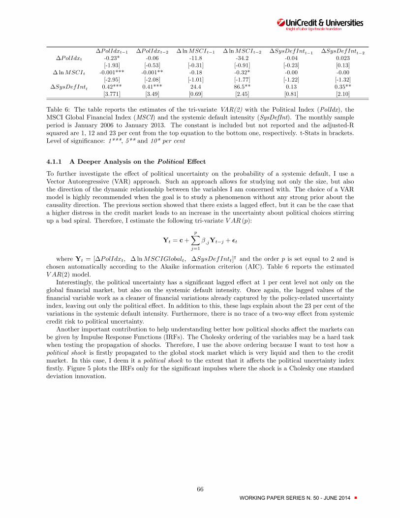
�PolIdxt�1 �PolIdxt�2 �lnMSCIt�1 �lnMSCIt�2 �SysDefIntt�1 �SysDefIntt�2�PolIdxt -0.23* -0.06 -11.8 -34.2 -0.04 0.023

[-1.93] [-0.53] [-0.31] [-0.91] [-0.23] [0.13]�lnMSCIt -0.001*** -0.001** -0.18 -0.32* -0.00 -0.00

[-2.95] [-2.08] [-1.01] [-1.77] [-1.22] [-1.32]�SysDefIntt 0.42*** 0.41*** 24.4 86.5** 0.13 0.35**

[3.771] [3.49] [0.69] [2.45] [0.81] [2.10]

Table 6: The table reports the estimates of the tri-variate VAR(2) with the Political Index (PolIdx), theMSCI Global Financial Index (MSCI) and the systemic default intensity (SysDefInt). The monthly sampleperiod is January 2006 to January 2013. The constant is included but not reported and the adjusted-Rsquared are 1, 12 and 23 per cent from the top equation to the bottom one, respectively. t-Stats in brackets.Level of signi�cance: 1***, 5** and 10* per cent

4.1.1 A Deeper Analysis on the Political E¤ect

To further investigate the e¤ect of political uncertainty on the probability of a systemic default, I use aVector Autoregressive (VAR) approach. Such an approach allows for studying not only the size, but alsothe direction of the dynamic relationship between the variables I am concerned with. The choice of a VARmodel is highly recommended when the goal is to study a phenomenon without any strong prior about thecausality direction. The previous section showed that there exists a lagged e¤ect, but it can be the case thata higher distress in the credit market leads to an increase in the uncertainty about political choices stirringup a bad spiral. Therefore, I estimate the following tri-variate V AR (p):

Yt = c+

pXj=1

�;jYt�j + �t

where Yt = [�PolIdxt; � lnMSCIGlobalt; �SysDefIntt]| and the order p is set equal to 2 and is

chosen automatically according to the Akaike information criterion (AIC). Table 6 reports the estimatedV AR(2) model.

Interestingly, the political uncertainty has a signi�cant lagged e¤ect at 1 per cent level not only on theglobal �nancial market, but also on the systemic default intensity. Once again, the lagged values of the�nancial variable work as a cleaner of �nancial variations already captured by the policy-related uncertaintyindex, leaving out only the political e¤ect. In addition to this, these lags explain about the 23 per cent of thevariations in the systemic default intensity. Furthermore, there is no trace of a two-way e¤ect from systemiccredit risk to political uncertainty.

Another important contribution to help understanding better how political shocks a¤ect the markets canbe given by Impulse Response Functions (IRFs). The Cholesky ordering of the variables may be a hard taskwhen testing the propagation of shocks. Therefore, I use the above ordering because I want to test how apolitical shock is �rstly propagated to the global stock market which is very liquid and then to the creditmarket. In this case, I deem it a political shock to the extent that it a¤ects the political uncertainty index�rstly. Figure 5 plots the IRFs only for the signi�cant impulses where the shock is a Cholesky one standarddeviation innovation.


1 2 3 4 5 6 7 8 9 100.06

0.04

0.02

0

0.02Response of MSCI Global Index to Political Uncertainty

1 2 3 4 5 6 7 8 9 105

0

5

10

15Response of Sys temic Default Intens ity to Political Unc ertainty

1 2 3 4 5 6 7 8 9 1020

10

0

10Response of Sys temic Default Intens ity to MSCI Global Index

Figure 5. Impulse Response Functions computed from the estimated tri-variate VAR(2 ) over the monthlysample period January 2006 to January 2013. The responses are a Cholesky one standard deviation

innovations. The grey area corresponds to the con�dence intervals at twice the standard errors. Only thesigni�cant responses are reported.

The �rst two IRFs in Figure 5 plots the response of the changes in the systemic default intensity toa political and a �nancial shock. The probability of a systemic breakdown reacts positively to politicalshocks with this e¤ect living for three months. Interestingly, the political shock dominates the �nancialone to the extent that it survives for longer. Moreover, as the third graph shows, the political shock hasalso a contemporaneous impact on the global �nancial market. In conclusion, since Figure 5 plots onlythe signi�cant responses, there is no evidence of a reverse causality from the credit market to the politicaluncertainty which could have exasperated the crisis.

4.2 Is the European Crisis a Debt Crisis?

As a result of the �nancial crisis 2007/09, the wave of bailouts made by governments has led to a signi�cantincrease in the sovereign debts. Thus, I believe that a higher indebtness is a signal of a more likely systemicdefault. In order to investigate such a relationship, I exploit the cross section of the 24 European countriesand test the signi�cance of the linkage between the two main observed ratios, namely, the debt over GDPand the bank asset over GDP from January 2006 to January 2013. These two ratios have a clear economicmeaning. The former measures the degree of indebtness of a country with respect to its own economy. Thebank asset over GDP ratio measures, instead, the ability of a country to rescue its own banking system incase of default. Figure 1 already drew a dramatic scenario where the most indebted countries have hugebanking systems with respect to their economies.

Such a linkage has already been investigated by Dieckmann and Plank (2012) and Acharya et al. (2011)but not from a cross sectional point of view which gives a time-varying measure of the e¤ect. In fact, theformer study the determinants of CDS spreads during the mid-2007 �nancial crisis for 18 European developedeconomies. They argue that the size and the pre-crisis health of both the world and country�s �nancial marketpositively a¤ect the CDS spread. Moreover, they stress the potential role of the private-to-public risk transferchannel - that is, more government guarantees on the �nancial sectors, signi�cant extension of loans�amountto the banking system, etc. - which allows investors to form expectations about future �nancial bailouts.Acharya et al. (2011) which �rst models and then tests the two-way feedback e¤ect between the sovereigncredit risk and �nancial markets. When a sovereign comes into play to rescue its insolvent �nancial systemwith a debt expansion �nanced by taxes, it induces a positive signal in the market which then turns into a


negative one owing to an increase in the marginal cost of raising the tax revenue (La¤er curve) and a morelimited maximum debt capacity. Hence, a distressed sovereign may exacerbate the �nancial sector�s solvencycondition since it would no longer be able to make any transfer.

Therefore, for each time step I run the following regressions separately:

Yt = �t + �t �BankAsset=GDPt�1 + tD �BankAsset=GDPt�1 (9)

Yt = �t + �t �Debt=GDPt�1 + tD �Debt=GDPt�1 (10)

where Yt is the cross section of the default intensities scaled by the standard deviations4 , the �s are thecoe¢ cients of interest and D is a dummy variable which takes the value of one for the countries with low andmedium debt over GDP ratios, such as Cyprus, United Kingdom, France, Belgium, Ireland, Portugal, Italyand Greece. Therefore, � captures the relationship between the most indebted European countries and thedefault intensity. Equation 9 is on a monthly basis and the weekly intensities of default are aggregated bypicking up the central week of each month. Instead, equation 10 is on a quarterly basis. In addition to this,both ratios are lagged because of release issues of such statistics.

Figure 5 plots the �s and their con�dence intervals at 95 per cent level of signi�cance.

0 10 20 30 40 50 60 70 80 900.6

0.4

0.2

0

0.2

0.4Bank Asset/GDP (Panel A)

0 5 10 15 20 25 300.06

0.04

0.02

0

0.02

0.04Debt/GDP (Panel B)

Figure 5. Cross sectional coe¢ cients of the regressions of Bank Asset over GDP ratio (monthly data)(Panel A) and Debt over GDP ratio (quarterly data) (Panel B) on the default intensities of the 24European countries. The sample period is January 2006 to January 2013. Grey areas are 95 per cent

con�dence intervals.

Both panels display the same path. Interestingly, Panel B highlights a negative and signi�cant relationshipduring the �nancial crisis 2007/09, namely, higher sovereign debt is associated with lower credit risk. It maybe the case that higher indebteness was perceived positively by the markets to the extent that it signalledthe willingness of countries to bailout their banking systems. But, then, after the �nancial crises reached thehighest peak during the Lehman Brother default, the coe¢ cients show an upward trend. Such a relationshipis signi�cantly positive at the end of 2010 when a big debate about the �rst bailout in the European Unionhistory was in place, namely, the Greek bailout reached in May 2010. Results not reported here show thatEastern countries do not have such a positive and signi�cant relationship. Such a result is in line with whatFigure 3 already showed. In fact, Eastern countries that have low debt over GDP have su¤ered the most the�nancial crisis 2007/09 whose probability of default reached the highest peak during the Lehman bankruptcy.Moreover, these economies are performing better than the most developed European countries.

4The default intensities are scaled by the standard deviations to avoid that the exponential trend of the intensity of Greeceabsorbe the whole e¤ect.


In conclusion, the high indebtness, together with very large banking systems, are associated with sig-ni�cant amount of credit risk in Europe. Hence, policy interventions aimed at reducing the large debts, atrestoring growth rates and reaching a sort of political stability in the most developed European countriesmay contribute signi�cantly to reduce the probability of a systemic breakdown of the whole European Union.

5 Conclusions

What moves the systemic credit risk in Europe? This paper studies empirically the determining factors ofthe European credit market, exploring its systemic nature.

Using a cross section of 24 European countries as members of the European Union, I calibrate the Angand Longsta¤ (2011) Credit Default Swap pricing model to extract the common default intensity which givesa measure of the probability of a systemic breakdown of the European Union.

The novelty of this paper is to test how political uncertainty in�uences the systemic default intensity andto show how the European crisis 2010/13 is a debt crisis, that is, a high indebtness of a country, togetherwith a large banking system, compared to the size of the economy, are a signal of a higher probability of asystemic default.

The results in the this paper highlight two important aspects of the European Union. The �rst is relatedwith the fragile political environment which spreads out an amount of risk that increases signi�cantly theprobability of systemic breakdown, with devastating contagion e¤ects. Exemplar is the Summer 2011 whenresignations of the prime ministers in Italy and Greece and the threat of Euro-exit referendums leaded to adramatic increase in the probability of a systemic default as high as during the Lehman Brother bankruptcy.The second aspect is the high degree of heterogeneity among the EU members. In fact, the combination ofhigh indebtness and large banking systems in the most developed countries add up a certain riskiness because,together with poor performances in terms of GDP growth, they are more and more �nancially constrainedand so unable to bail out.

Policy interventions aimed at reducing the large debts, at restoring growth rates and reaching a sortof political stability in the most developed European countries may contribute signi�cantly to reduce theprobability of a systemic breakdown of the whole European Union. Indeed, concrete policy commitments bythe leading economies such as a permanent subsidizing, may be able to reach a certain stability calming themarkets down.


References

[1] Acharya, Viral V., Itamar Drechsler, and Philipp Schnabl. A pyrrhic victory?-bank bailouts and sovereigncredit risk. No. w17136. National Bureau of Economic Research, 2011.

[2] Ang, Andrew, and Francis A. Longsta¤. "Systemic sovereign credit risk: Lessons from the us andeurope." Journal of Monetary Economics (2013).

[3] Baker, Scott R., Nicholas Bloom, and Steven J. Davis, "Measuring economic policy uncertainty", Work-ing paper, Stanford University (2011).

[4] Boero, Gianna, Jeremy Smith, and Kenneth F. Wallis. "Uncertainty and Disagreement in EconomicPrediction: The Bank of England Survey of External Forecasters*." The Economic Journal 118.530(2008): 1107-1127.

[5] Bomberger, William A. "Disagreement as a Measure of Uncertainty." Journal of Money, Credit andBanking 28.3 (1996): 381-392.

[6] Carr, Peter, and Liuren Wu. "Stock options and credit default swaps: A joint framework for valuationand estimation." Journal of Financial Econometrics 8.4 (2010): 409-449.

[7] Carr, Peter, and Liuren Wu. "Theory and evidence on the dynamic interactions between sovereign creditdefault swaps and currency options." Journal of Banking & Finance 31.8 (2007): 2383-2403.

[8] Dieckmann, Stephan, and Thomas Plank. "Default risk of advanced economies: An empirical analysisof credit default swaps during the �nancial crisis." Review of Finance 16.4 (2012): 903-934.

[9] Du¢ e, Darrell, and Kenneth J. Singleton. Credit risk: pricing, measurement, and management. Prince-ton University Press, 2012.

[10] Hansen, Lars Peter, "Challenges in Identifying and Measuring Systemic Risk", University of ChicagoWorking Paper (2012)

[11] Lahiri, Kajal, and Xuguang Sheng. "Measuring forecast uncertainty by disagreement: The missing link."Journal of Applied Econometrics 25.4 (2010): 514-538.

[12] Longsta¤, Francis A., Jun Pan, Lasse H. Pedersen, and Kenneth J. Singleton. 2011. "How Sovereign IsSovereign Credit Risk?" American Economic Journal: Macroeconomics, 3(2): 75-103.

[13] Manzo, Gerardo and Antonio Picca, "The Sovereign Nature of Systemic Risk", Working Paper (2013)

[14] Manzo, Gerardo, "Political Uncertainty, Credit Risk Premium and Default Risk",Working Paper (2012)

[15] Pan, Jun, and Kenneth J. Singleton. "Default and recovery implicit in the term structure of sovereignCDS spreads." The Journal of Finance 63.5 (2008): 2345-2384.

[16] Pastor, Lubos, and Pietro Veronesi. "Uncertainty about government policy and stock prices." The Jour-nal of Finance 67.4 (2012): 1219-1264.

[17] Pastor, Lubos, and Pietro Veronesi. Political uncertainty and risk premia. No. w17464. National Bureauof Economic Research, 2011.

[18] Ulrich, Maxim. "How does the Bond Market Perceive Government Interventions?." Columbia BusinessSchool Research Paper 12/42 (2013).

[19] Wan, Eric A., and Rudolph Van Der Merwe. "The unscented Kalman �lter for nonlinear estimation."Adaptive Systems for Signal Processing, Communications, and Control Symposium 2000. AS-SPCC. TheIEEE 2000. IEEE, 2000.


The Sovereign Nature of Systemic Risk

Gerardo Manzo*

University of Rome "Tor Vergata"

University of Chicago Booth School of Business

Antonio Picca**

University of Chicago Booth School of Business

June 2013

Abstract

We study the impact of bank specific and sovereign specific shocks to systemic credit riskand analyze the contagion effect between two macro systems: the European sovereigns and theEuropean banking systems. We form portfolios of sovereign and bank debt and, using a Bayesiantechnique, we measure systemic risk as the premium an investor would pay for hedging tail losseson those portfolios. We then identify bank specific and sovereign specific shocks relying on thenarrative approach. Channels of contagion are studied according to a portfolio sorting approachwhere we sort European sovereigns according to their debt over GDP ratio and European banksaccording to their exposure to the most leveraged countries. We mainly find that the system ofsovereign spreads out a sort of systemic risk that cannot be neglected, especially if we realizethat the sovereign system is ultimately in charge of bailing out the banking system. From amacro prudential perspective as it suggests that the announcement of macro policies, aimed atmitigating sovereign systemic risk, also have a significant impact on banking systemic risk butnot vice-versa. Therefore, policies that target the sovereign system should be preferred overpolicies that target the banking system.

[JEL No. G12,G13,G18]

Keywords: Systemic Risk, Credit Default Swap, Importance Sampling, Narrative Ap-

proach, Banking System, Sovereign Debt, Financial Crisis

*[email protected] .Gerardo Manzo is a PhD candidate in Money and Finance at the University ofRome "Tor Vergata". The paper was written while Gerardo Manzo was a visiting scholar at The University of ChicagoBooth School of Business. **[email protected]. Antonio Picca is a PhD candidate in Finance andEconomics at the University of Chicago Booth School of Business. The authors are grateful to Pietro Veronesi, BryanKelly and Stefano Giglio for their invaluable comments. All errors are our responsibility.


1 Introduction

The ongoing financial crisis, which began in mid-2007 with the crash of the US housing-bubble,

has triggered a wave of sovereign debt-increases in the Euro zone.

Governments have been forced to lever up to prevent the collapse of their own financial and

banking systems. The growing amount of debt has resulted in a rapid widening of European

countries’ credit spreads. Thus, difficulties in rolling-over the debt on capital markets have arisen,

requiring the intervention of supranational entities, such as the ECB, IMF and World Bank. The

consequent high volatility in the European credit market has laid the basis for analyzing the systemic

nature of credit risk. Although there is no common definition of systemic risk, generally speaking, it

is meant to be the risk of a disorderly and catastrophic breakdown of a whole macroeconomic region,

such as the European Union. Even if the interconnectedness of a banking system is a precondition

for a quicker and more severe contagion throughout the system, a simultaneous breakdown of

sovereigns may exacerbate the distress, making interventions by local governments impossible.

This very predicament has been brought to fruition in many areas throughout Europe. Large

countries’ indebtedness, sluggish growth rates, reduced power of monetary institutions due to low

interest rates and overused quantitative easing, raising inflation rates caused by austerity plans and

Middle-East geopolitical risks (higher commodity prices) have made a disorderly breakdown of the

whole macroeconomic region more likely .

In this work we study the impact of bank specific and sovereign specific shocks to systemic credit

risk and analyze the contagion effect between two macro systems: the European sovereigns and the

European banking systems. Differently from previous studies (Black et al. (2013), Acharya et al.

(2012), Tarashev et al. (2009), among others) that focus only on the banking sector to analyze the

risk of a systemic collapse, we also look at the risk embedded in sovereign debts, as we believe that

shocks to sovereign systemic risk might influence the stability of the financial system and hence

have an effect on the banking sector. In addition to this, we also study the channels of contagion

between the two systems.

We form portfolios of sovereign and bank debt and we measure systemic risk as the premium an

investor would pay for hedging tail losses on this portfolio. Given the rare nature of these events,

estimating their probabilities is particularly challenging as a common Monte Carlo approach has


been proved to be inefficient, thus the estimation requires more sophisticated econometric tools.

To this extent, we use Importance Sampling, a Bayesian technique which changes the probability

measure under which the premium is priced in order to make rare events more likely. Besides

being less computationally intensive, such a technique yields a more efficient estimator than the

plain Monte Carlo method. Moreover, this measure is basically a risk-neutral expectation of the

portfolio loss conditional on the loss being in the tail of the distribution. Therefore, this is a

coherent credit risk measure as opposed to the classical value-at-risk and hence it works well with

a portfolio sorting approach to the extent that the subadditivity property applies..

In order to study the impact of sovereign and bank specific shocks, we rely on the narrative

approach of Romer and Romer (1989). According to this approach, we can identify and separate

shocks to the banking sector from shocks to sovereigns and their directional effect by looking at

relevant news on a specific day. We can also label shocks to the extent that we can directly

distinguish shocks that affect only sovereigns from shocks that affect only banks. The use of this

narrative approach is dictated by the complex and relatively unexplored nature of the relation

between sovereign and banking systemic risk that makes statistical approaches such as Cholesky

ordering, long-run constraints, and sign restrictions not economically justifiable.

Finally, using a portfolio sorting approach, we identify the channels of contagion. We sort

European sovereigns according to their debt over GDP ratio and European banks according to

their exposure to the most leveraged countries such as the PIIGS (Portugal, Ireland, Italy, Greece

and Spain). We believe that, in a highly levered macro region such as the European Union, debt

over GDP captures the cross-sectional variation in reaction of sovereigns to sovereign shocks. In

fact, the more levered countries are the ones more in need of financial support from the EU and

hence are more exposed to the shocks affecting the stability of the sovereign system. Similarly we

believe that the second ratio captures, at the same time, different risk exposures and cross-sectional

variation in implicit guarantees.

Several findings emerge from this analysis: we find that the effect of sovereign shocks on banking

systemic risk in around 0.6 on impact and it is strongly significant whose effect persist for two days.

Such a result is in line with our belief, that is, the system of sovereign spreads out a sort of systemic

risk that cannot be neglected, especially if we realize that the sovereign system is ultimately in

charge of bailing out the banking system; in addition to this, the portfolio approach tells us that


countries with large debt to GDP ratio suffered the most sovereign shocks. This is in line with

the view that high debts add up a significant fragility in the system of sovereign, making potential

bailouts more difficult to be achieved; finally, banks of the most leveraged countries that are more

exposed to their domestic sovereign debt are also the ones that have the weakest implicit guarantee

of being bailed out, thus„ suffering the most sovereign shocks.

The paper proceeds as follows: we discuss the methodology used to measure the systemic credit

risk in Section 2; Section 3 introduces the data; then, we present the narrative approach in Section

4 together with empirical findings, and Section 5 concludes the analysis.

2 Systemic Credit Risk Measure

The systemic risk methodology is built according to a portfolio credit risk management methodol-

ogy.

Assuming that there exists a hypothetical investor who holds a portfolio on liabilities of N

credits, the systemic risk indicator emerges as a hypothetical insurance premium the investor is

willing to pay for hedging against catastrophic losses. A similar approach has been used by Black

et al. (2013) in relation to a portfolio of European banks. We believe that such an approach has

limited advantages when used in the context of a single portfolios but it has a great advantage when

it comes to analyze different portfolios and sub-portfolios. Therefore, we consider two portfolios as

representatives of two major financial systems: the European sovereign system and the European

banking system.

At the core of the insurance premium there is the tail loss probability, namely, the probability

of having a loss greater than an exogenous amount which we set equal to 10 per cent1. Consider a

portfolio consisting of public debts of N credits, and let Li denote the loss on credit i’s debt with

i = 1, ..., N . Then, L = ∑Ni=1 Li is the total loss of the portfolio. Therefore, the insurance premium

is basically the expected loss conditional on the loss exceeding a certain threshold x, that is,

EQ[L|L ≥ x] (1)

where the expectation is taken under the risk-neutral probabilities. Indeed, as we shall show, the1The results are robust to different threshold levels such as 15 or 20 per cent.


default probabilities are extracted from credit default swap spread.

2.1 Tail Probability: Importance Sampling

The expectation in equation 1 embeds the probability of the loss being in the tail, that is, it requires

the estimation of low-probability events of large losses. The classical Monte Carlo simulation

method alone is known not to be accurate in estimating equation 1, especially for very large values

of x. Glasserman and Li (2005) and Grundke (2009) propose an alternative way to estimate the

tail loss probability based on two step Importance Sampling (IS) which reduces the variance of

the estimator by changing the probability measure from which paths are generated, such that

“important” events have more weight.

Hence, for a clear representation of the procedure, we report the IS methodology in details.

2.1.1 Portfolio Credit Risk

The portfolio approach described here is one of the classical bottom-up approaches, that is, it

consists in piecing together subsystems to give rise to larger systems.

Let us consider the following notation:

N : number of credits in the portfolio,

Yi: default indicator (=1 if i-th credit defaults),

PDi: marginal default probability of i-th credit,

ELGDi: expected Loss Given Default of i-th credit,

L = ELGD1Y1 + ...+ ELGDNYN : Aggregate portfolio loss,

where PDi and ELGDi are assumed known a priori.

The tail probability is then estimated according to the Importance Sampling method whose

main advantage is to get a more efficient estimator with less simulations than the plain Monte Carlo

approach. In fact, the main contribution of IS is to increase the marginal default probabilities when

the total loss of the portfolio is not in the tail of the distribution. Thus, each marginal default

probability for the entry i at time t, PDi,t, is replaced by some twisted ones, PDi,t(θ), such that

the tail probability is as follows


Pr(L ≥ x) = EQ[1 {L≥x}]

= EQ

1 {L≥x}N∏i=1

(PDi,t

PDi,t(θ)

)Yi(

1− PDi,t

1− PDi,t(θ)

)1−Yi (2)

where the second expectation is still risk-neutral but now under then new probability measure and

adjusted by the likelihood ratio. The latter keeps the identity holding for the two expectations, EQ

and EQ.

2.1.2 Exponential Twisting

The first step of IS is concerned with choosing a functional form for the twisting. Following

Glasserman and Li (2005), we use the exponential twisting where each marginal default probability

is twisted by a single parameter θ ≥ 0 such that the new probability is equal to

PDi,t(θ) = PDi,texp(θ×ELGDi)1 + PDi,t(exp(θ×ELGDi)− 1) (3)

Using the exponentially twisted probabilities, the likelihood ratio in 2 simplifies to

1 {L≥x}N∏i=1

(PDi,t

PDi,t(θ)

)Yi(

1− PDi,t

1− PDi,t(θ)

)1−Yi

= 1 {L≥x} exp(−θL+ ψ(θ)), (4)

where

ψ(θ) =N∑i=1

log(1 + PDi,t(exp(θ × ELGDi)− 1)).

is the cumulant generating function2.

The choice of θ depends on whether we are in the tail or not. If L > x a tail loss is not rare,

so we set θ = 0, that implies PDi,t(θ) = PDi,t. If L < x a tail loss is rare, so θis optimally chosen

to make a tail loss more likely. In this case, our choice of θ minimizes the second moment of the

estimator Pr(L ≥ x). Conveniently, it turns out that the optimal choice of θ is such that Eθ[L] = x.

Therefore, θ can be interpreted as the parameter that shifts the distribution of L so that x is now2Just as the generating function M of a random variable X “generates” its moments, the logarithm of M generates a

sequence of numbers called the cumulants of X. It incorporates important information on the probability distribution,namely, its first derivatives is the mean of the distribution.


its new mean.

Equation 4 shows that exponentially twisting the probabilities is equivalent to applying an

exponential twist to L itself.

2.1.3 Conditional Importance Sampling

The second step of the IS deals with the simulations of the losses whose joint default probabilities

are caught by the Normal Copula model.

A default occurs when a random variable falls below a certain threshold which is chosen to

match the marginal probability of default of each credit. Using the implications of Merton (1974),

a default occurs when the stock log-return falls below such a threshold, namely,

Yi,t = 1 {Ri,t < yi,t}

where Ri,t is the log-return of the credit i at time t, and the threshold yi,t = Φ−1(PDi,t), with Φ

being the cumulative standard Normal distribution. In order to introduce the dependence among

the entries of the portfolio, we assume that the stock return is driven by F common factors,

Mt = [M1,t, ...,MF,t]T and an idiosyncratic factor, Zi,t as follows

Ri,t = BiMt +√

1−BiBTi ·Zi,t (5)

where Bi = [bi,1, ..., bi,F ] is the vector of loadings with bi,f ∈ [−1, 1] and ∑Ff=1 bi,f

2 ≤ 1.

Therefore, the conditional probability of default, conditional on the realization of the common

factor Mt = mt is

PDi,t(mt) = Pr (Yi,t = 1|Mt = mt)

= Pr (Ri,t < yi,t|Mt = mt)

= Pr

(BiMt +

√1−BiBT

i · Zi,t < yi,t|Mt = mt

)

= Φ

yi,t −Bimt√1−BiBT

i

(6)

Given the assumptions of the Normal Copula model presented in equation 5, each realizations


mt of the factors Mt is drawn from a multivariate normal with mean mt and unit variance. The

choice of the mean vector m is the second step of the IS procedure. We set an optimal mf,t for each

factor f and time t. As shown in Glasserman and Li (2005), an optimal choice of m greatly reduces

the variance of the tail probability estimator, Pr(L ≥ x) 3.

Thus, the conditional expected loss is

EQ[Lt|Mt = mt] =N∑i=1

PDi,t(mt)× ELGDi,t.

2.1.4 Simulation Approach

Using the exponential twisting enables us to get the conditional twisted probabilities, PDi,t(mt,j)

which are then used to draw default scenarios Yi,t from a Bernoulli distribution with parameter

PDi,t(mt, θ). We repeat this procedure 500, 000 times for each time period t. This approach

gives us a vector Yt of defaults for each time period t and each simulation. Given that the loss

given default is not known a priori, we further simulate 50 loss scenarios for each of our previous

simulations. We draw loss scenarios from a triangular distribution 4. If ELGDi,t is at least 0.6,

we draw LGDi,t from a symmetric triangular distribution with mean equal to ELGDi,t and in

the range [2 × ELGDi,t − 1, 1]. If ELGDi,t is less than 0.6, we draw LGDi,t from an asymmetric

triangular distribution with mode equal to ELGDi,t and in the range [0, 1]. Then, the total loss

for each simulated scenario is

Lt =N∑i=1

Yi,t × LGDi,t.

Then, averaging the above equation across the different loss scenarios leads to 500, 000 portfolio

losses for each time period t. The insurance premium can now be computed as

EQt [Lt|Lt≥x] = EQt [Lt×1 {Lt≥x}] (7)

= EQt

[Lt×1 {Lt≥x} exp(−θ(mt)Lt + ψ(θ(mt),mt))exp(−µTt mt + ((µTt µt)/2))

]

where the last expectation is taken under then new probability measure. The term inside the3See Glasserman and Li (2005) for a more detailed discussion of the procedure used to compute m.4The triangular distribution assumption is for computational convenience as shown by Tarashev and Zhu (2009b).


expectation is the likelihood ratio associated with the new measure. Specifically, the new likelihood

ratio has two components: the first exponential is the likelihood ratio of the first IS step, as in

equation 4, while the second exponential is the likelihood ratio of the second IS step. Once again,

the likelihood ratio adjustment enables us to keep the identity between the different probability

frameworks.

2.2 Inputs of the Portfolio Approach

To compute the expectation in equation 7, we assume that the default probabilities and the stock

market loadings are known. Therefore, we calibrate both inputs with market data. Assuming a

Poisson distribution for the default probability, we extract the embedded risk-neutral intensity of

default from Credit Default Swap (CDS) spread. This extraction is performed by calibrating the

Pan and Singleton (2008) pricing model where the default intensity follows a log-normal process.

Then, the default probability for the credit i at time t is PDi,t = 1 − e−lQi,t , where lQi,t is the

risk-neutral default intensity5.

While CDS spreads embed credit risk information, the stock market correlation catches the

degree of interconnectedness of the financial markets and so it is used to calibrate the loading

of the factor model. This calibration follows Andersen et al. (2003). Thus, factor loadings are

estimated by minimizing the distance between the empirical and the simulated correlation matrix.

Given these two main inputs, we are now able to apply the above methodology.

3 Data

The two portfolios are composed of 24 European countries and 41 European banks, respectively.

For each asset in the portfolio we collect CDS spreads, expected recovery rates, total liabilities and

stock prices.

CDS spreads are collected from the Markit database. These are daily spreads for the maturities

1-, 2-, 3-, 5- and 7-year covering the period from July 3, 2006 to January 22, 2013. For sovereigns

we use spreads with a complete restructuring (CR) clause, while for the European banks we use

spreads with a modified-modified restructuring (MM) clause. The CR and the MM clauses agree5A table with the calibrated parameters is not reported here but it can be obtained upon request.


on the definition of credit events but differ on the maturity of the deliverable obligation. According

to the CR clause any bond of maturity up to 30 years is deliverable. According to the MM clause

deliverable obligations against the contract have to be limited to those with a maturity of 60 months

or less after the termination date of the CDS contract. Our choice of data is constrained by their

availability and by concerns about liquidity. Besides, Markit provides also measures of expected

recovery rates which are used only for a simulation purpose, as already explained. In addition to

CDS spreads, we collect stock market data for each entry with the same frequency as CDS spreads

and over the same time period. More specifically, we use local stock indices for countries and

individual stocks for banks. Finally, since we are dealing with portfolios of liabilities, we collect

country public consolidated debt from Eurostat and banks’ total liabilities from Datastream.

Table 1 and Table 2 report a list of the countries and of the banks of our portfolios, together

with summary statistics6. As we can see from Table 1, there is a high degree of heterogeneity

across countries. In fact, Greece shows the most worrying condition with an average spread of

about 1053 bps, meaning that an investor is willing to pay more than 10 percent of his notional of a

portfolio of Greek debt to hedge against a default. Moreover, the term structure slopes, computed

as the difference between the 7-year and the 1-year spread, depict inverted markets for the most

worrying countries such as Cyprus, Greece, Ireland and Portugal. This means that the market

expects, on average, high default probabilities in the short-run for these countries. Moreover, the

standard deviations and the autocorrelations show a high variability across countries and a high

degree of persistence of the time series, respectively. Table 2 reports the same statistics for the

pool of European banks. The credit worthiness of the European banking system resembles in part

that of their countries. Indeed, the banks of the most worrying countries have experienced, on

average, larger spreads than the others, with the Greek banks followed by the Irish, Spanish and

Italian ones. Moreover, all the Greek banks in our sample have negative term slopes, together with

the Bank of Ireland. Such a picture depicts a strict relationship between the country and its own

banking system which is in charge of bailing out in case of a default.

Figure 1 plots the average daily pairwise correlation for the two systems. The correlation is

commonly used as a measure of contagion across markets to the extent that a shock is propagated6Given the large amount of data we report only the main statistics. Additional information is available upon

request.


quickly when the degree of correlation is high. In fact, during period of high turmoil the two series

spike. Interestingly, the picture depicts how the beginning of the wave of bailouts by governments

during the Lehman default contributed significantly to increase the degree of contagion in the

sovereign system. This scenario is clear highlighted by the sudden and wide increase in the sovereign

correlation at the beginning of September 2008 when correlations were as high as 50 per cent for

sovereigns and 63 per cent for banks.

The last set of data regards liabilities for each entry of the portfolios. For sovereigns, we

collect the public consolidated debt figures reported by Eurostat. Eurostat reports these figures at

quarterly frequencies and converts them to Euros for extra-EMU countries. European banks’ total

liabilities are collected from Datastream. Figure 2 shows both total liabilities (line) and year on year

variations of liabilities (bars) grouped by regions. Panel A plots countries liabilities. We observe a

steady increase in public debt across the three macro-areas since 2008, accompanying the wave of

bailouts. The variations in extra-EMU countries liabilities are not directly comparable because of

variations in exchange rates. The 2008 drop in liabilities is caused by several devaluations of extra-

EMU currencies against the Euro. At the same time, the 2009 increase in liabilities is exacerbated

by a rebound of those currencies against the Euro. In panel B we observe a pronounced increase

in bank liabilities in 2006 as a consequence of a wave of cross-border bank consolidations7. In 2010

bank liabilities plummeted as a consequence of deleveraging efforts following the new regulation on

capital requirements.

3.1 Systemic Credit Risk

Given the data and the methodology in Section 2, the systemic credit risk is measured for European

sovereigns and European banks.

Figure 3 plots the sovereign insurance premium in basis points. Sovereign systemic risk starts

increasing right after the Lehman Brother default when interventions by European supranational

institutions such as ECB were implemented for the first time. Thereafter, a sequence of political

and economic events have contributed to push up the risk throughout Europe. In fact, the end of

2009 can be deemed as the beginning of the European debt crisis when doubts arose around the

feasibility of the first bailout in the European Union history, namely, the Greek bailout that was7As an example, BNP paid 9bn EUR to acquire BNL.


reached in May 2010. The Summer 2011 is particularly interesting since the systemic risk reached

the highest levels as a consequence of political turmoils in Italy, Greece and Spain. Moreover, as we

can see, announcements of policy interventions by ECB and EU are associated with large variations

in the systemic credit risk.

Figure 4 draws the banking insurance premium in basis points. The scenario is slightly different

from the sovereign one. Indeed, the first part of the sample, namely, the financial crisis 2007/09,

is characterized by large variations as a result of the large wave in the US banking system. The

bank insurance premium starts increasing in August 2007 and peaks for the first time in March

2008, around Bearn Sterns’s debacle. Interestingly, ECB interventions have contributed mitigating

the systemic risk thanks to the implementation of policies such as extraordinary liquidity measures

and bond purchase programme. All these interventions aimed at restoring a certain liquidity in the

bond market which experienced a significant crunch because of the high countries’ indebtedness.

In order to have a more general picture, figure 5 plots both insurance premiums. The first

part of the sample coincides with the financial crisis of 2007/09, when the risk was mostly driven

by the instability of the financial sector and spillovers from the US banking system. The second

part of the sample coincides with the sovereign crisis of 2010/13, when the joint instability of the

sovereign and the financial sector drove the systemic credit risk. Moreover, after the second big

spike in the banking risk in September 2008 when Lehman failed, it is evident a sort of risk transfer

from the banking system to the sovereign one. It is clear from the graph that in September 2008

there is a marked divergence between bank and sovereign premiums due mostly to the perceived

risk transfer, from banks to sovereigns. Such a risk transfer is a consequence of the wave of bailouts

and of the ECB’s and Fed’s effort to provide liquidity to the short-term founding market. Then,

the sovereign risk widens around the first Greek bailout and dominates for almost all the rest of

the sample. In June 2011, amid the political turmoils in Greece, Italy, Spain and Belgium, there is

a sudden spike in the sovereign insurance premium, shortly followed by the bank one, that rose by

2% in few months.


4 Empirical Framework

This section shall introduce first the methodology used to study the impact of bank specific and

sovereign specific shocks on the systemic credit risk and, then, the procedure implemented to

identify shocks through a coherent and systematic way. We start by considering a 2-dimensional

vector autoregressive model

yt = Φy(L)yt−1 + Φxxt + ut,

where yt is a vector containing the daily first differences of the sovereign and the bank insurance

premium, Φy(L) = ∑Jj=1 Φy,jL

j−1 is a polynomial of 2 × 2 matrices in the lag operator, xt is

an m-dimensional vector of exogenous variables that includes the constant, and ut is a vector of

innovations. In a more compact form, this model can be written as

yt = Φzt + ut, (8)

where zt = [y′t−1, ..., y′t−J , x

′t] is a p × 1 vector of both lagged endogenous and exogenous variables

with p = 2J +m and Φ = [Φy,1, ...,Φy,J ,Φx] is an 2× p matrix of coefficients.

The innovations ut are jointly correlated reflecting the spillovers between sovereign and banking

systemic risk. Following standard practice, we assume

ut = Bεt, (9)

where εt is an i.i.d. vector of specific shocks with zero mean. The matrix B therefore reflects the

rate of transmission of these shocks across systems. Without loss of generality, we normalize the

diagonal elements of B to one, which reflect the within-system transmission of shocks.

4.1 Narrative Approach

Given the complex and relatively unexplored nature of the relation between sovereign and banking

systemic risk we cannot rely on statistical approaches to identify the off-diagonal elements of the

matrix B. Cholesky ordering, exclusion restrictions, sign restrictions and long-run constraints do

not have enough economic support to be used in this case. To get around this problem we use

a narrative approach similar to Romer and Romer (1989). As part of this approach, we first


decompose each country-specific shock into a signed mean shift, which shall reflect “exceptional”

and to some extent observable events, and a residual noise, which shall reflect “normal” shocks.

Specifically, we assume for each system i that

εi,t = di,tξi + νi,t,

where di,t ∈ {−1, 0, 1} is a signed indicator for exceptional events affecting directly the system i,

ξi denotes the average size of the exceptional events, νi,t reflects the normal events, and di,t and

νi,t are i.i.d. across time and systems8. Applying the same decomposition to each system, we can

rewrite

εt = Dtξ + νt,

where Dt is a 2×2 diagonal matrix with entries di,t; εt and νt are 2×1 vectors; and ξ = [ξsov, ξbk]T

is a 2× 1 vector of average size of the exceptional events for the sovereign and the banking system,

respectively.

The narrative approach allows us to identify a specific set of dates where exceptional shocks hit

either the banking system or the sovereign system, and to determine the sign of of the corresponding

shock. Using this information, we can define signed indicator functions 1sov,t and 1bk,t. We can

then rewrite the vector of system specific shocks as

εt = 1tξ + νt, (10)

where 1t is a diagonal matrix, whose diagonal elements are 1sov,t and 1bk,t.

4.2 Shock Identification

In order to identify the exceptional shocks, we collect daily relevant news from a variety of sources

such as Financial Times, Wall Street Journal, Wikipedia, BBC, Reuters, Bloomberg, rating agency

website, ECB, Brugel and the Saint Louis Fed. According to our selection criterion, a news is rele-

vant when it includes: i) policy announcement and implementation from Central Banks, European

Union and individual countries; ii) rating agencies’ actions; iii) social unrest; and iv) extraordinary8The i.i.d. assumption does not change our results but makes the notation conveniently simpler. All the results

reported here are corrected for autocorrelation through block-bootstrap.


events such as bankruptcy, bailouts and nationalizations.

We identify two macro categories of shocks: shock generator and shock recipient. The former can

be the European Central Bank, the European Union, foreign institutions (Fed, US Treasury) and

rating agencies. These are basically institutions which have the power of reverting negative trends

and of mitigating the risk in financial markets, thus, generating the shocks. The shock recipient is

essentially that system directly affected by shocks. In particular, we distinguish between banking

and sovereign specific shocks. In our identification, one shock hits either the banking system or the

sovereign system. There are only a few days when a shock hits both systems. Examples of these

are the announcement of a monetary policy in support of both systems, the sovereign bailout of a

bank or the joint downgrade of a country and its banking system.

The narrative approach requires also to identify the direction of the shock. As explained in

section 4.1 we measure shocks using a categorical variables that takes value of one if the shock

is supposed to mitigate the risk and increase the stability of that system. Examples of positive

shocks to sovereigns are the announcement and approvals of austerity plans, bailouts by the EU,

and upgrades by rating agencies. Conversely, examples of negative shocks to sovereigns are social

unrest, political instability or electoral uncertainty, rating downgrades, request of a bailout and

rescue of a domestic bank. Table 3 reports the two macro categories of shocks: generators and

recipients in panel A and B, respectively. Moreover, the square brackets report the direction of the

shock. The time line is reported in the online Appendix.

As a practical example, on March 15, 2010 the finance ministers of the EU agreed on a mech-

anism to help Greece. This is a positive shock generated by the EU and received by the sovereign

system. On February 10, 2012, Standard and Poors downgraded 37 Italian banks. This is a negative

shock generated by a rating agency and received by the banking system.

4.3 Aggregate Results

As mentioned above, we want to study the rate of transmission of shocks across systems. In order

to do this we build a bivariate VAR with 3 lags9, with sovereign and banking insurance premiums as

endogenous variables. The lags enable us to control for that information which is already included

in the market. The regressions are performed on first differences as they have a clear economic9The number of lags is automatically chosen according to the Akaike Information Criteria


interpretation. Indeed, a reduction of the insurance of 3 bps on a notional of 1, 000, 000$, means

that we save 300$ per year to insure our portfolio against losses higher than 100, 000$. The results

are robust to the use of log returns but in this case the coefficients do not have such an intuitive

economic interpretation10. More specifically, we run OLS regressions as follows:

yt = Φy(L)yt−1 + Φxxt + βsov1sov,t + βbk1bk,t + et, (11)

where Φy(L) = ∑3j=1 Φy,jL

j−1 is a polynomial of 2 × 2 matrices in the lag operator; xt is an

3-dimensional vector of exogenous variables that includes the constant, a dummy for the Euro-

pean sovereign debt crisis, and the lagged first difference of the US banking systemic insurance

premium11; βsov = [βsov,sov, βbk,sov]′ is a 2 × 1 vector of loadings on sovereign exceptional shocks;

βbk = [βsov,bk, βbk,bk]′ is a 2× 1 vector of loadings on banking exceptional shocks; and et is a vector

of innovations.

Combining equation 8 with equations 9 and 10 we have that

yt = Φzt +B1tξ +Bνt. (12)

Comparing the above to the regressions in equation 11 and imposing the restriction on the diagonal

elements of the matrix B, we have that βsov,sov = ξsov, βbk,bk = ξbk,β

bk,sov = Bbk,sovξsov and

βsov,bk = Bsov,bkξbk, where BY,X indicates the effect of the X-shock onto the system Y .These

results imply that the off-diagonal elements of the B matrix can be computed as

Bsov,bk = βsov,bk/βbk,bk,

Bbk,sov = βbk,sov/βsov,sov,

so, using the narrative approach, we can identify the rate of transmission of these shocks across

systems. An analytical confidence intervals for these ratios cannot be easily computed, therefore10Logarithms are often used in the bond literature since log returns are equivalent to first differences in the yield.

Our insurance premium is economically similar to a CDS and so, in line with the CDS literature, we use firstdifferences.

11The US systemic insurance premium is computed using a portfolio of 19 US banks. The data are the same asthe ones used for the European systems and are collected from the same sources. We do not report detailed statisticsabout these data since our main focus is Europe. These statistics can be obtained upon request. The idea is tocorroborate our results controlling for possible spillover effect from the US economy.


we rely on block-bootstrapping techniques to construct empirically consistent confidence intervals

for Bsov,bk and Bbk,sov.

Table 4 reports the estimated value for ξsov, ξbk, Bsov,bk andBbk,sov . The confidence intervals are

estimated using 1, 000 bootstrap simulations, with a 5-day blocks to account for the autocorrelation

of the residuals. We see that ξsov and ξbk, the average size of the mean shifting shocks, are

respectively −3.34 and −3.69, meaning that a positive exceptional shock on average reduces the

insurance premium by more than 3 bps and this effect is strongly significant. Looking at Bsov,bk

and Bbk,sov we see that the coefficients are positive but less than one. This means that positive

shocks to one system reduces systemic risk in the other but it is not transmitted one-to-one across

systems. Moreover, we see that shocks to the sovereign system have a large and strongly significant

impact on banking systemic risk, while shocks to the banking system have a small and almost

insignificant impact on the sovereign system.

The impulse response functions plotted in Figure 6 give us a clearer picture. The figure reports

the impulse response function and the 95% bootstrapped confidence intervals. We see that the effect

of banking shocks on sovereign systemic risk is around 0.3 on impact but almost not significant.

We also see that the effect decays immediately. On the other hand, the effect of sovereign shocks

on banking systemic risk is around 0.6 on impact and it is strongly significant, with the lower

confidence interval at 0.4. Moreover, the effect persists for two days.

These results are in line with our belief, that is, the system of sovereign spreads out a sort

of systemic risk that cannot be neglected, especially if we realize that the sovereign system is

ultimately in charge of bailing out the banking system. This finding has an interesting application

from a macro prudential perspective as it suggests that the announcement of macro policies aimed

at mitigating sovereign systemic risk also have a significant impact on banking systemic risk but

not vice-versa. Therefore, policies that target the sovereign system should be preferred over policies

that target the banking system. Since the beginning of the financial crisis, the European leaders

have been talking about a mechanism to shore up banks directly, without guarantying countries.

In view of our results, this mechanism might not be able to decrease banking systemic risk since

the sovereign one adds up significant systemic risk.


4.4 Portfolio Approach Sovereigns

The results presented in section 4.3 suggest that shocks to the sovereign system have a large and

strongly significant impact on banking systemic risk. To better identify the channel of transmission

of these shocks across systems we study the relation between sovereign systemic risk and banking

systemic risk. To do this we use a portfolio approach where we form three portfolios of sovereign

liabilities sorted on their debt to GDP ratio and three portfolios of banking liabilities sorted on

exposure to countries with large debt to GDP ratio. Our hypothesis is that countries with the

largest debt to GDP ratio and banks with a large exposure to these countries suffered the most

sovereign shocks.

4.4.1 Sovereigns

In this section we form three portfolios of sovereign liabilities sorted on their debt to GDP ratio.

For each portfolio i of sovereigns we run a 2-dimensional VAR similar to the one described by

equation 11. In particular, we run a VAR that has the insurance premium for portfolio i of

sovereigns and the aggregate banking insurance premium as endogenous variables. This implies

that βsov = [βsovi,sov, βbk,sov]′ is a 2 × 1 vector of loadings on sovereign exceptional shocks; βbk =

[βsovi,bk, βbk,bk]′ is a 2× 1 vector of loadings on banking exceptional shocks. We are now interested

in identifying the first row of the B matrix, namely Bsovi,sov and Bsovi,bk. Since our regression uses

shocks to the aggregate sovereign system, a reasoning similar to the one of section 4.3 tells us that

βsovi,sov = Bsovi,sovξsov and βsovi,bk = Bsovi,bkξbk, and thus

Bsovi,sov = βsovi,sov/βsov,sov,

Bsovi,bk = βsovi,bk/βbk,bk.

Table 4 shows the coefficients for Bsovi,sov and Bsovi,bk together with the 95% bootstrapped

confidence intervals and p-values. However, a clearer picture is given by the impulse response

functions reported in Figure 7, panel A. The figure reports the impulse response functions and the

95% bootstrapped confidence intervals for, respectively, portfolio 1, 2 and 3. Portfolio 1 is the one

with lowest debt to GDP ratio and includes the Baltic and Eastern European countries. Portfolio


3 is the one with the highest ratio and includes most of the PIIGS countries (Portugal, Ireland,

Italy, Greece, Spain) with the exception of Spain, together with France, Cyprus, Belgium, and

Malta. The portfolios are rebalanced annually using the previous year’s consolidated public debt

and GDP figures, however there is a little portfolio migration. Only Ireland moved from portfolio

1 to 3 across the sample period.

We see that the effect of banking shocks on sovereign systemic risk is only significant for port-

folio 1. However the confidence intervals largely overlap across the three portfolios, meaning that

this ratio does not capture cross-sectional variation in reaction of sovereigns to banking shocks.

Conversely, the cross-sectional variation in reaction of sovereigns to sovereign shocks is well cap-

tured by this ratio. Indeed, the portfolios are ranked in increasing order, with little to no overlap

of confidence intervals. This result tells us that countries with large debt to GDP ratio suffer the

most sovereign shocks. This is in line with the view that states that high leveraged countries are

more fragile. In fact, these countries are the ones more in need of financial support from the EU

and hence are more exposed to the shocks affecting the stability of the sovereign system.

4.4.2 Banks

In this section we form three portfolios of banking liabilities sorted on banks’ exposure to countries

with large debt to GDP ratio. For each portfolio i of banks we run a 2-dimensional VAR similar

to the one described by equation 11. In particular, we run a VAR that has the aggregate sovereign

DIP and the DIP for portfolio i of banks as endogenous variables. This implies that βsov =

[βsov,sov, βbki,sov]′ is a 2×1 vector of loadings on sovereign exceptional shocks; βbk = [βsov,bk, βbki,bk]′

is a 2 × 1 vector of loadings on banking exceptional shocks. We are now interested in identifying

the second row of the B matrix, namely Bbki,sov and Bbki,bk. Using a reasoning similar to the one

used above we can easily see that βbki,sov = Bbki,sovξsov and βbki,bk = Bbki,bkξbk, and thus

Bbki,sov = βbki,sov/βsov,sov,

Bbki,bk = βbki,bk/βbk,bk.

Table 4 shows the coefficients for Bbki,sov and Bbki,bk together with the 95% bootstrapped


confidence intervals and p-values. However, a clearer picture is given by the impulse response

functions reported in Figure 7, panel B. The figure reports the impulse response functions and the

95% bootstrapped confidence intervals for, respectively, portfolio 1, 2 and 3. Portfolio 1 is the one

with the lowest exposure to countries with high debt to GDP ratio and includes British banks,

northern European banks and the biggest Spanish banks. Portfolio 3 is the one with the highest

exposure to countries with high debt to GDP ratio and includes French, Italian, Irish and Greek

banks. The portfolios are static as figures on direct exposure of European banks to each European

country’s debt are only available for December 201012. The sorting is done on the ratio of long

exposure to countries in sovereign portfolio 3 over total long exposure.

We see that the effect of banking shocks is significant on every portfolio, however the confidence

intervals largely overlap across the three portfolios, meaning that this ratio does not capture cross-

sectional variation in reaction of banks to banking shocks. Conversely, the cross-sectional variation

in reaction of banks to sovereign shocks is well captured by this ratio. Indeed, the portfolios are

ranked in increasing order, with little overlap of confidence intervals. This result tells us that banks

with exposure to countries with large debt to GDP ratio suffered the most sovereign shocks. Such

a finding can be explained in two ways. First of all, these banks have a large exposure to the

countries that suffer the most sovereign shocks and hence their assets are more sensitive to these

shocks. However, looking at the composition of the portfolios, we notice that portfolio 3 includes

almost exclusively Italian, Irish and Greek banks, and these banks have a very large domestic

exposure. Therefore, we can say that these are banks whose implicit guarantees are largely affected

by sovereign systemic risk.

5 Conclusion

This work addresses an important and not so much explored issue, that is, it deals with the impact

of bank specific and sovereign specific shocks to systemic credit risk and analyzes the contagion

effect between two macro systems: the European sovereigns and the European banking system.

After introducing a coherent methodology to measure the systemic credit risk perceived by the

market, we rely on the narrative approach of Romer and Romer (1989) in order to identify and12The data were published by the European Banking Authority as part of the 2011 EU-wide stress test.


label bank and sovereign specific shocks. The main contribution of this paper is to show how the

economic conditions of the system of sovereigns has been driving the credit risk in Europe since the

beginning of debt crisis in 2010. In fact, in an environment of high indebted countries that are in

charge of bailing out their own banking systems, the policy-maker’s primary goal has to be aimed

at restoring the financial stability of the system of sovereigns. Indeed, the main finding suggests

that the announcement of macro policies aimed at mitigating sovereign systemic risk also have a

significant impact on banking systemic risk but not vice-versa.

Our next goal is to study the dynamics of the systemic credit risk premium embedded in the

term structure of Credit Default Swap spreads. In order to extract such a premium, we will build a

pricing model equivalent to the one exposed in Section 2, whose systemic default intensity follows

a lognormal process à la Pan and Singleton (2008). Understanding what moves investors’ risk

aversion may be of crucial importance for the policy-maker in identifying the right strategies in

order to mitigate the systemic credit risk and corroborate the anti-fragility of a complex system,

that is, the European sovereign system.

References

Acharya, Viral V & Pedersen, Lasse H & Philippon, Thomas & Richardson, Matthew P, (2012).

"Measuring Systemic Risk," CEPR Discussion Papers 8824, C.E.P.R. Discussion Papers.

Grundke, Peter, (2009). "Importance sampling for integrated market and credit portfolio mod-

els," European Journal of Operational Research, Elsevier, vol. 194(1), pages 206-226, April.

Acharya, Viral V. & Drechsler, Itamar & Schnabl, Philipp, (2011). "A Pyrrhic Victory? - Bank

Bailouts and Sovereign Credit Risk," NBER Working Paper, No. 17136.

Bekaert, Geert & Wu, Guojun, (2000). "Asymmetric Volatility and Risk in Equity Markets,"

Review of Financial Studies, Oxford University Press for Society for Financial Studies, vol. 13(1),

pages 1-42.

Andersen, L., J. Sidenius and S. Basu, (2003). “All your Hedges in One Basket”, RISK,

November, 67-72.

Tarashev, Nikola, Claudio Borio, and Kostas Tsatsaronis (2009b). “The systemic importance

of financial institutions,” BIS Quarterly Review.


Longstaff, Francis A., Jun Pan, Lasse H. Pedersen, and Kenneth J. Singleton. (2011). "How

Sovereign Is Sovereign Credit Risk?." American Economic Journal: Macroeconomics, 3(2): 75-103.

Ang, Andrew, & Longstaff, Francis A. (2011), “Systemic sovereign credit risk: Lessons from the

US and Europe” (No. w16982). National Bureau of Economic Research.

Pan, Jun, and Kenneth J. Singleton. (2008). "Default and recovery implicit in the term structure

of sovereign CDS spreads." The Journal of Finance 63.5: 2345-2384.

Glasserman, Paul, and Jingyi Li. (2005) "Importance sampling for portfolio credit risk." Man-

agement science 51.11: 1643-1656.

Black, Lamont, Ricardo Correa, Xin Huang, Hao Zhou. (2013). “The systemic risk of European

banks during the financial and sovereign debt crisis”. Federal Reserve Board Washington.

Brutti, Filippo, and Philip Sauré. (2011) "Transmission of sovereign risk in the euro crisis."

Available at SSRN 2041257.

Romer, Christina D., and David H. Romer. (1989). "Does monetary policy matter? A new

test in the spirit of Friedman and Schwartz." NBER Macroeconomics Annual 1989, Volume 4. MIT

Press. 121-184.

Merton, Robert C. (1974) "On the pricing of corporate debt: The risk structure of interest

rates*." The Journal of Finance 29.2: 449-470.


Table 1: Summary Statistics - Sovereigns

The table reports summary statistics of daily sovereign Credit Default Swap spreads over the period July3, 2006 to January 22, 2013. Min, Mean, Max are the minimum, the average and the maximum value ofthe 5-year CDS spread, respectively. Slope is the difference between the 7-year and the 1-year CDS spread,namely, the slope of the term structure. Std Dev is the standard deviation and AC is the AutoCorrelationfunction. All the statistics are reported in basis points.

Min Mean Max Slope (7y-1y) Std Dev AC

Austria 1 56.6 269 27.5 50.0 0.995Belgium 2 75.0 339 30.5 69.4 0.995Bulgaria 13 209.3 687 71.1 142.8 0.997Cyprus 5 317.2 1601 -35.6 436.6 0.997

Czech Rep 5 76.6 350 39.8 58.2 0.996Denmark 1 41.8 149 24.6 39.8 0.998Estonia 6 142.4 736 38.6 151.7 0.998Finland 1 28.4 92 17.0 23.9 0.996France 1 46.7 199 26.7 41.1 0.992

Germany 1 25.7 91 17.7 20.0 0.993Greece 5 1053.8 23572 -3112.7 2458.9 0.957Ireland 2 263.7 1263 -11.3 273.7 0.999Italy 5 137.4 502 40.5 127.0 0.997Latvia 5 288.7 1161 34.0 245.8 0.998

Lithuania 6 217.9 849 44.6 174.2 0.998Malta 5 141.8 466 28.2 129.7 0.998

Netherlands 1 34.1 130 18.3 29.3 0.992Poland 8 117.2 419 59.9 83.1 0.996Portugal 4 306.4 1554 -37.8 377.3 0.999Slovakia 5 88.5 297 45.1 73.4 0.997Slovenia 3 108.3 471 47.4 116.0 0.998Spain 2 138.9 504 36.6 123.4 0.997Sweden 1 31.6 158 18.1 30.0 0.997UK 1 49.3 165 31.0 36.6 0.997


Table 2: Summary Statistics - Banks

The table reports summary statistics of daily bank Credit Default Swap spreads over the period July 3, 2006to January 22, 2013 grouped by their home country. Min, Mean, Max are the minimum, the average andthe maximum value of the 5-year CDS spread, respectively. Slope is the difference between the 7-year andthe 1-year CDS spread, namely, the slope of the term structure. Std Dev is the standard deviation and ACis the AutoCorrelation function. All the statistics are reported in basis points.

Min Mean Max Slope (7y-1y) Std Dev AC

AustriaErste Group 10 151.0 483 40.3 98.8 0.997

Raiffeisen Zentralbank 10 155.7 528 44.3 98.7 0.997

BelgiumDexia 6 299.1 947 13.0 255.2 0.998KBC 7 163.1 495 39.8 117.3 0.998

Denmark Danske 4 109.8 330 39.8 87.2 0.999

France

BNP Paribas 5 95.8 361 42.2 77.2 0.996Credit Agricole 6 118.3 401 46.8 87.8 0.996Societe Generale 6 124.0 433 45.9 99.5 0.996

Natixis 7 149.4 336 35.6 90.5 0.997

Greece

Alpha Bank 15 745.0 3025 -346.1 782.5 0.997Eurobank Ergasias 14 738.8 2836 -346.4 784.1 0.997

National Bank of Greece 11 708.7 2791 -346.6 765.5 0.995Piraeus Bank 18 748.5 2800 -285.8 789.8 0.996

GermanyIKB Deutsche Industriebank 11 375.3 1412 -34.2 279.2 0.998

Commerzbank 8 114.6 364 46.0 82.1 0.996Deutsche Bank 9 97.5 318 45.8 56.3 0.993

Ireland Gov & Co Bank of Ireland 6 443.7 2033 -116.8 445.0 0.995

Italy

Banca Monte dei Paschi di Siena 6 197.7 880 37.0 204.6 0.998Banca Popolare di Milano 11 191.0 842 35.7 210.4 0.998

UniCredit 7 167.3 692 40.6 152.8 0.997Unione di banche italiane 11 166.8 683 40.3 152.5 0.997

Intesa Sanpaolo 6 145.0 625 38.8 144.0 0.998

NetherlandsING Groep 4 103.2 274 38.3 66.7 0.994

Van Lanschot Bankiers 18 157.9 357 20.6 92.8 0.997Norway DNB Bank 8 77.5 204 36.0 48.8 0.997

Spain

Bco Bilbao Vizcaya Argentaria 8 159.6 510 47.1 129.1 0.997Banco de Sabadell 9 292.1 854 31.5 233.5 0.998

Banco Popolar Espanol 8 295.4 897 28.9 250.2 0.999Banco SANTANDER 8 152.2 490 47.3 121.6 0.997

Bankinter 11 268.9 858 37.8 212.1 0.998

Sweden

Nordea Bank 5 76.4 202 35.9 47.6 0.997Skandinaviska Enskilda Banken 7 101.6 258 36.9 63.4 0.998

Svenska Handelsbanken 5 65.6 170 29.8 40.3 0.998Swedbank 5 116.1 367 39.0 79.4 0.996

SwitzerlandCredit Suisse Group 9 95.0 261 42.0 54.2 0.994

UBS 4 108.5 357 41.3 69.7 0.994

UK

Barclays Bank 5 113.2 285 46.5 68.3 0.994HSBC 5 83.5 202 36.2 47.0 0.992

LLOYDS TSB Bank 4 139.9 391 49.2 98.7 0.997Royal Bank of Scotland 4 151.1 403 51.8 100.1 0.995Standard Chartered 6 95.5 354 38.7 63.2 0.995


Table 3: Mean Shifting Shocks

The table reports the Shock Generator (Panel A) and the Shock Recipient (Panel B). The former are theinstitutions that are able to generate shocks throguh both announcements and actions, such as, ECB, EUand Rating Agencies. The Shock Recipient are the systems which are directly affected by these shocks. Theshock identification is based on relevant news collected from newspapers. In particular, each panel reportsthe general content of a news, such as monetary policy expansion, lack of commitment, etc. The squarebrackets show the direction of the shock: -1 for negative shocks to the economy, +1 positive shocks.


Table 4: Shock Transmission

The table reports the estimated value for ξsov and ξbk, that represent the average size of the mean shiftingshocks, and the elements of the matrix B, that reflects the rate of transmission of shocks within and acrosssystems. The sovereign portfolios are sorted on debt to GDP ratio, in increasing order. The banking portfoliosare sorted on exposure to countries with high debt to GDP ratio, in increasing order. BY,X indicates theeffect of the X-specific shock on the system Y . The confidence intervals and the p-values are estimated using1, 000 bootstrap simulations, with a 5-day blocks to account for autocorrelation of the residuals.

Coefficient 95% CI p-value

Aggregate

ξsov -3.34 -4.67 -2.05 0.000ξbk -3.69 -5.08 -2.41 0.000

Bsov,bk 0.29 0.00 0.53 0.049Bbk,sov 0.61 0.42 0.76 0.000

Sovereign Portfolios

Bsov1,sov 0.54 0.40 0.74 0.000Bsov2,sov 0.88 0.72 1.02 0.000Bsov3,sov 2.02 1.81 2.25 0.000Bsov1,bk 0.52 0.23 0.87 0.000Bsov2,bk 0.21 -0.09 0.48 0.158Bsov3,bk 0.53 0.03 1.02 0.037

Bank Portfolios

Bbk1,sov 0.46 0.18 0.67 0.004Bbk2,sov 0.84 0.59 1.04 0.000Bbk3,sov 1.26 0.66 1.82 0.000Bbk1,bk 1.33 1.05 1.65 0.000Bbk2,bk 1.10 0.98 1.21 0.000Bbk3,bk 1.09 0.60 1.53 0.001


Figure 1: Stock Market Correlation

The figure plots the daily stock logreturns correlations computed according to a one-year rolling window.The two lines represent the equally-weighted average of pairwise correlations for countries (solid line) andfor banks (dashed line). For countries we look at the local stock market indices. For financial conglomerateswe take the stock price of the holding group as we believe it to be a better proxy for the financial stabilityof the company. The sample period covers July 3, 2006 to January 22, 2013.


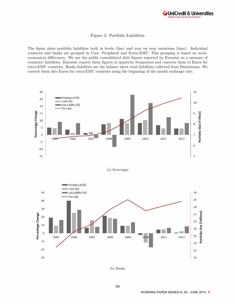
Figure 2: Portfolio Liabilities

The figure plots portfolio liabilities both in levels (line) and year on year variations (bars). Individualcountries and banks are grouped in Core, Peripheral and Extra-EMU. This grouping is based on socio-economical differences. We use the public consolidated debt figures reported by Eurostat as a measure ofcountries’ liabilities. Eurostat reports these figures at quarterly frequencies and converts them to Euros forextra-EMU countries. Banks liabilities are the balance sheet total liabilities collected from Datastream. Weconvert them into Euros for extra-EMU countries using the beginning of the month exchange rate.

(a) Sovereigns

(b) Banks


Figu

re3:

SovereignSy

stem

icRisk

The

figureplotsthean

nual

insuranc

eprem

ium

inba

sispo

ints

forapo

rtfolio

ofEu

rope

ansovereignlia

bilities.

The

prem

ium

isrepo

rted

atda

ilyfre

quencies

andis

equivalent

tothean

nual

prem

ium

that

aninvestor

wouldpa

yto

hedg

eagainstaloss

high

erthan

10%

onhispo

rtfolio

.The

figure

also

repo

rtssomeof

thekeyevents

that

hadalargeim

pact

onsovereignde

bt.


Figu

re4:

Bank

ingSy

stem

icRisk

The

figureplotsthean

nual

insuranc

eprem

ium

inba

sispo

ints

forapo

rtfolio

ofEu

rope

anba

nkinglia

bilities.

The

prem

ium

isrepo

rted

atda

ilyfre

quencies

andis

equivalent

tothean

nual

prem

ium

that

aninvestor

wouldpa

yto

hedg

eagainstaloss

high

erthan

10%

onhispo

rtfolio

.The

figure

also

repo

rtssomeof

thekeyevents

that

hadalargeim

pact

onba

nkingde

bt.


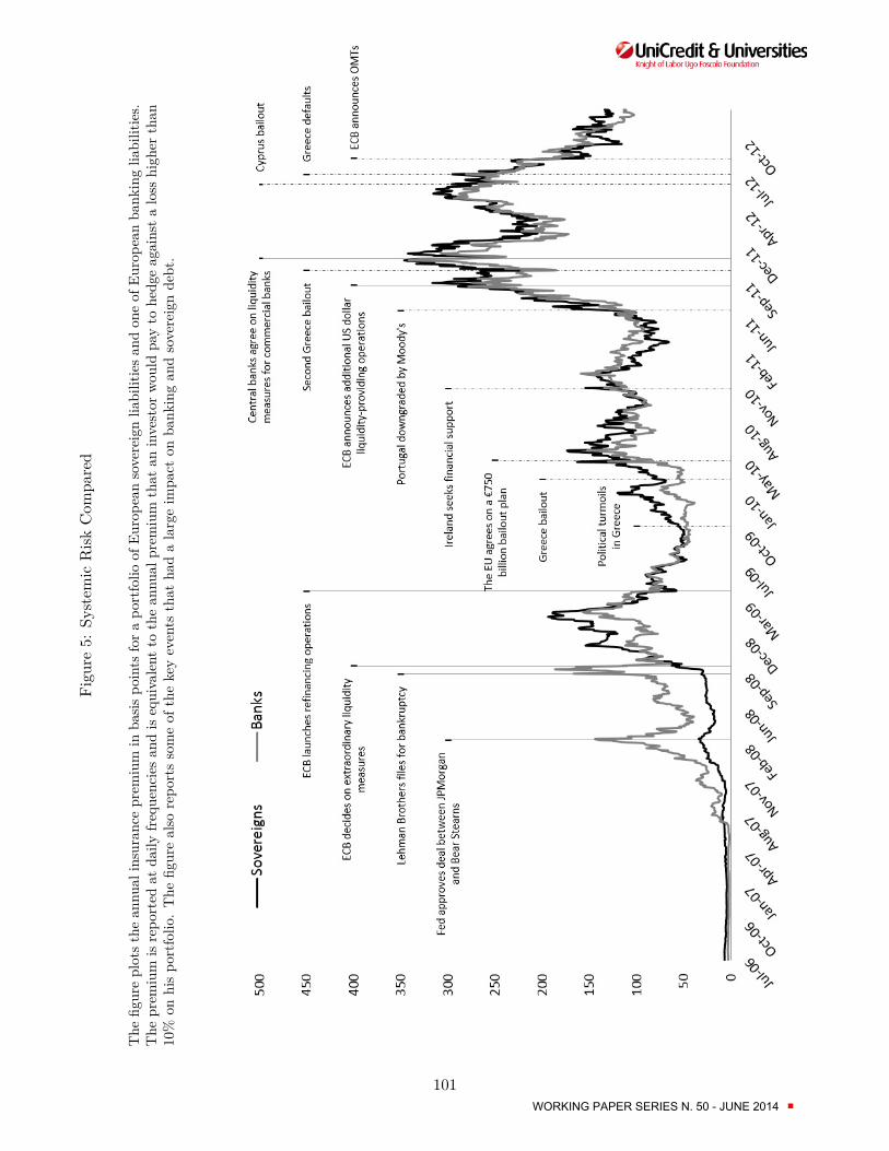
Figu

re5:

System

icRisk

Com

pared

The

figureplotst

hean

nual

insuranc

eprem

ium

inba

sispo

ints

fora

portfolio

ofEu

rope

ansovereignlia

bilitiesa

ndon

eof

Europe

anba

nkinglia

bilities.

The

prem

ium

isrepo

rted

atda

ilyfre

quencies

andisequivalent

tothean

nual

prem

ium

that

aninvestor

wouldpa

yto

hedg

eag

ainsta

loss

high

erthan

10%

onhispo

rtfolio

.The

figurealso

repo

rtssomeof

thekeyevents

that

hadalargeim

pact

onba

nkingan

dsovereigndebt.


Figure 6: Aggregate Impulse Response Functions

The figure plots the Impulse Response Functions of sovereign systemic risk to banking shocks and of bankingsystemic risk to sovereign shocks. These impulse response functions capture the transmission of shocks acrosssystems. The confidence intervals are estimated using 1, 000 bootstrap simulations, with a 5-day blocks toaccount for auto correlation of residuals.


Figure 7: Portfolios Impulse Response Functions

The figure draws Impulse Response Functions for the sorted portfolios. Panel A plots the impulse responsefunctions of sovereign portfolios to sovereign and banking shocks. The portfolios are sorted on debt to GDPratio, in increasing order. Panel B plots the impulse response functions of bank portfolios to sovereignand banking shocks. The portfolios are sorted on exposure to countries with high debt to GDP ratio, inincreasing order. The confidence intervals are estimated using 1, 000 bootstrap simulations, with a 5-dayblocks to account for auto correlation of residuals.

(a) Sovereign Portfolios

(b) Bank Portfolios



UniCredit & Universities

Knight of Labor Ugo Foscolo Foundation

Piazza Gae Aulenti – UniCredit Tower, Torre A

20154 Milan

Italy

Giannantonio De Roni – Secretary General

[email protected]

Annalisa Aleati - Scientific Director

[email protected]

Info at:

[email protected]

www.unicreditanduniversities.eu

http://www.unicreditanduniversities.eu/

what drives systemic risk? political uncertainty and ... · working paper series n. 50 june 2014...

Documents