Infinite matroids in graphs

Henning Bruhn Reinhard Diestel

Abstract

It has recently been shown that infinite matroids can be axiomatized in away that is very similar to finite matroids and permits duality. This waspreviously thought impossible, since finitary infinite matroids must havenon-finitary duals.

In this paper we illustrate the new theory by exhibiting its implicationsfor the cycle and bond matroids of infinite graphs. We also describetheir algebraic cycle matroids, those whose circuits are the finite cyclesand double rays, and determine their duals. Finally, we give a su�cientcondition for a matroid to be representable in a sense adapted to infinitematroids. Which graphic matroids are representable in this sense remainsan open question.

1 Introduction

In the current literature on matroids, infinite matroids are usually ignored, orelse defined like finite ones1 with the following additional axiom:

(I4) An infinite set is independent as soon as all its finite subsets are indepen-dent.

We shall call such set systems finitary matroids.The additional axiom (I4) reflects the notion of linear independence in vector

spaces, and also the absence of (finite) circuits from a set of edges in a graph.More generally, it is a direct consequence of (I4) that circuits, defined as minimaldependent sets, are finite.

An important and regrettable consequence of the additional axiom (I4) isthat it spoils duality, one of the key features of finite matroid theory. Forexample, the cocircuits of an infinite uniform matroid of rank k would be thesets missing exactly k � 1 points; since these sets are infinite, however, theycannot be the circuits of another finitary matroid. Similarly, every bond of aninfinite graph would be a circuit in any dual of its cycle matroid—a set of edgesminimal with the property of containing an edge from every spanning tree—butthese sets can be infinite and hence will not be the circuits of a finitary matroid.

1The augmentation axiom is required only for finite sets: given independent sets I, I0 with|I| < |I0| < 1, there is an x 2 I0 r I such that I + x is again independent.

1

This situation prompted Rado in 1966 to ask for the development of a theoryof non-finitary infinite matroids with duality [15, Problem P531]. In the late1960s and 70s, a number of such theories were proposed; see [3] for references.One of these, the ‘B-matroids’ proposed by Higgs [12], were later shown byOxley [13] to describe the models of any theory of infinite matroids that admittedboth duality and minors as we know them. However, Higgs did not presenthis ‘B-matroids’ in terms of axioms similar to those for finite matroids. Asa consequence, theorems about finite matroids whose proofs rested on theseaxioms could not be readily extended to infinite matroids, even when this mighthave been possible in principle.

With the axioms from [3] presented in the next section, this could nowchange: it should be possible now to extend many more results about finitematroids to infinite matroids, either by

• adapting their proofs based on the finite axioms to the (very similar) newinfinite axioms,

or by

• finding a sequence of finite matroids that has the given infinite matroidas a limit, and is chosen in such a way that the instances of the theoremknown for those finite matroids imply a corresponding assertion for thelimit matroid.

After presenting our new axioms in Section 2, we apply them in Sections 3and 4 to see what they mean for graphs. We shall see that, for matroids whosecircuits are the (usual finite) cycles of a graph, our axioms preserve what wouldbe wrecked by the finitary axiom (I4): that their duals are the matroids whosecircuits are the bonds of our graph – even though these can now be infinite.

The converse is also nice. The dual M⇤ of the (finitary) matroid M whosecircuits are the finite bonds of an infinite graph cannot be finitary; indeed,trivial exceptions aside, the duals of finitary matroids are never finitary [19, 1];see also [5]. So M⇤ will have to have infinite circuits.2 Excitingly, these circuitsturn out to be familiar objects: when the graph is locally finite, they are the edgesets of the topological circles in its Freudenthal compactification, which alreadyhave a fixed place in infinite graph theory quite independently of matroids [8].

We shall see further that, for planar graphs, matroid duality is now fullycompatible with graph duality as explored in [2]. And Whitney’s theorem, thata graph is planar if and only if its cycle matroid has a graphic dual, now has aninfinite version too.

In some infinite graphs G, including all locally finite ones, the elementaryalgebraic cycles3 form the circuits of a matroid, the algebraic cycle matroidof G. We introduce this matroid, which was already studied by Higgs [11], inSection 3. In Section 5, we determine its dual.

2We are using here that every dependent set contains a minimal such. This is indeed true.3These are the minimal 1-chains (possibly infinite) with zero boundary: the edge sets of

finite cycles and of 2-way infinite paths.

2

In Section 6, finally, we consider representability. Infinite matroids that arerepresentable in the usual sense are finitary, and hence cannot have representableduals. We suggest an adapted notion of representability based on infinite sumsof functions to a field, and establish a su�cient condition for when this defines amatroid. Examples include the algebraic cycle matroids of graphs introduced inSection 3, and the algebraic cycle matroids of higher-dimensional complexes [3].

2 Axioms

We now present our five sets of axioms for finite or infinite matroids, in termsof independent sets, bases, circuits, closure and rank. These axioms were firststated in [3], and proved to be equivalent to each other in the usual sense. Forfinite or finitary matroids they coincide with the usual finite matroid axioms.

Let E be any set, finite or infinite; it will be the default ground set for allmatroids considered in this paper. We write 2E for its power set. The set ofall pairs (A,B) such that B ✓ A ✓ E will be denoted by (2E ⇥ 2E)✓; for itselements we usually write (A|B) instead of (A,B). Unless otherwise mentioned,the terms ‘minimal’ and ‘maximal’ refer to set inclusion. Given E ✓ 2E , wewrite Emax for the set of maximal elements of E , and dEe for the down-closureof E , the set of subsets of elements of E . For F ✓ E and x 2 E, we abbreviateF r{x} to F �x and F [{x} to F +x. We shall not distinguish between infinitecardinalities and denote all these by 1; in particular, we shall write |A| = |B|for any two infinite sets A and B. The set N contains 0.

One central axiom that features in all our axiom systems is that every in-dependent set extends to a maximal one, even inside any restriction X ✓ E.4The notion of what constitutes an independent set, however, will depend on thetype of axioms under consideration. We therefore state this extension axiom ina more general form first, without reference to independence, so as to be ableto refer to it later from within di↵erent contexts.

Let I ✓ 2E . The following statement describes a possible property of I.

(M) Whenever I ✓ X ✓ E and I 2 I, the set { I 0 2 I | I ✓ I 0 ✓ X } has amaximal element.

Note that the maximal superset of I in I\2X whose existence is asserted in (M)need not lie in Imax.

2.1 Independence axioms

The following statements about a subset I of 2E are our independence axioms:

(I1) ; 2 I.

(I2) dIe = I, that is, I is closed under taking subsets.4Interestingly, we shall not need to require that every dependent set contains a minimal

dependent set. We need that too, but it follows [3].

3

(I3) For all I 2 IrImax and I 0 2 Imax, there is an x 2 I 0rI such that I+x 2 I.

(IM) I satisfies (M).

When a set I ✓ 2E satisfies the independence axioms, we call the pair (E, I)a matroid on E. We call every element of I an independent set, every elementof 2E rI a dependent set, the maximal independent sets bases, and the minimaldependent sets circuits. This matroid is finitary if it also satisfies (I4) from theIntroduction, which is equivalent to requiring that every circuit be finite [3].

The 2E ! 2E function mapping a set X ✓ E to the set

cl(X) := X [ {x | 9 I ✓ X : I 2 I but I + x /2 I }

will be called the closure operator on 2E associated with I.The (2E ⇥ 2E)✓ ! N [ {1} function r that maps a pair A ◆ B of subsets

of E to

r(A|B) := max { |I r J | : I ◆ J, I 2 I \ 2A, J maximal in I \ 2B}

will be called the relative rank function on the subsets of E associated with I.This maximum is always attained, and independent of the choice of J [3].

2.2 Basis axioms

The following statements about a set B ✓ 2E are our basis axioms:

(B1) B 6= ;.

(B2) Whenever B1, B2 2 B and x 2 B1 r B2, there is an element y of B2 r B1

such that (B1 � x) + y 2 B.

(BM) The set I := dBe of all B-independent sets satisfies (M).

2.3 Closure axioms

The following statements about a function cl : 2E ! 2E are our closure axioms:

(CL1) For all X ✓ E we have X ✓ cl(X).

(CL2) For all X ✓ Y ✓ E we have cl(X) ✓ cl(Y ).

(CL3) For all X ✓ E we have cl(cl(X)) = cl(X).

(CL4) For all Z ✓ E and x, y 2 E, if y 2 cl(Z + x) r cl(Z) then x 2 cl(Z + y).

(CLM) The set I of all cl-independent sets satisfies (M). These are the sets I ✓ Esuch that x /2 cl(I � x) for all x 2 I.

4

2.4 Circuit axioms

The following statements about a set C ✓ 2E are our circuit axioms:

(C1) ; /2 C.

(C2) No element of C is a subset of another.

(C3) Whenever X ✓ C 2 C and (Cx | x 2 X) is a family of elements of C suchthat x 2 Cy , x = y for all x, y 2 X, then for every z 2 C r

�Sx2X Cx

�there exists an element C0 2 C such that z 2 C0 ✓

�C [

Sx2X Cx

�r X.

(CM) The set I of all C-independent sets satisfies (M). These are the sets I ✓ Esuch that C 6✓ I for all C 2 C.

Axiom (C3) coincides for |X| = 1 with the usual (‘strong’) circuit eliminationaxiom for finite matroids. In particular, it implies that adding an element toa basis creates at most one circuit; the fact that it does create such a (funda-mental) circuit is trivial when bases are defined from these circuit axioms (asmaximal sets not containing a circuit), while if we start from the independenceaxioms it follows from the fact, mentioned before, that every dependent setcontains a minimal one [3]. We remark that the usual finite circuit eliminationaxiom is too weak to guarantee a matroid [3].

2.5 Rank axioms

The following statements about a function r : (2E ⇥ 2E)✓ ! N [ {1} are our(relative) rank axioms:

(R1) For all B ✓ A ✓ E we have r(A|B) |A r B|.

(R2) For all A,B ✓ E we have r(A|A \B) � r(A [B|B).

(R3) For all C ✓ B ✓ A ✓ E we have r(A|C) = r(A|B) + r(B|C).

(R4) For all families (A�) and B such that B ✓ A� ✓ E and r(A� |B) = 0 forall �, we have r(A|B) = 0 for A :=

S� A� .

(RM) The set I of all r-independent sets satisfies (M). These are the sets I ✓ Esuch that r(I|I � x) > 0 for all x 2 I.

For finite matroids, these axioms (with (R4) and (RM) becoming redundant)are easily seen to be tantamount to the usual axioms for an absolute rank func-tion R derived as R(A) := r(A|;), or conversely with r(A|B) := R(A)�R(B)for B ✓ A.

5

3 Bond and cycle matroids

In this section we develop the theory of our axioms to see what it yields for theusual matroids for graphs when these are infinite. See [3] for applications toother structures than graphs. All our graphs may have parallel edges and loops.

A well-known matroid associated with a finite graph G is its cycle matroid:the matroid whose circuits are the edge sets of the cycles in G. The bases ofthis matroid are the edge sets of the spanning forests of G, the sets that forma spanning tree in every component of G. This construction works in infinitegraphs too: the edge sets of the finite cycles in G form the circuits of a finitarymatroid MFC(G), whose bases are the edge sets of the spanning forests of G. Weshall call MFC(G) the finite-cycle matroid of G. Similarly, we let the finite-bondmatroid MFB(G) of G be the matroid whose circuits are the finite bonds of G.(A bond is a minimal non-empty cut.) This, too, is a finitary matroid.

If G is finite, then MFC(G) and MFB(G) are dual to each other. For infi-nite G, however, things are di↵erent. As remarked earlier, the duals of finitarymatroids are not normally finitary, so the duals of MFC(G) and MFB(G) willin general have infinite circuits. In the case of MFC(G), its cocircuits are theexpected ones, the (finite or infinite) bonds:

Theorem 1. Let G be any graph.

(i) The bonds of G, finite or infinite, are the circuits of a matroid MB(G).

(ii) This matroid is the dual of the finite-cycle matroid MFC(G) of G.

The matroid MB(G) defined in Theorem 1 will be called the bond matroid of G.We defer the proof of the theorem to Section 4; it is essentially the same as forfinite graphs, although now the bonds can be infinite.

Similarly, the dual of MFB(G) will in general have infinite circuits. Ideally,these would form some sort of ‘infinite cycles’ in G. ‘Infinite cycles’ have indeedbeen considered before for graphs, though in a purely graph-theoretic context:there is a topological such notion that makes it possible to extend classicalresults about cycles in finite graphs (such as Hamilton cycles) to infinite graphs,see [8] and [17] in this issue. Rather strikingly, it turns out that these ‘infinitecycles’ are the solution also to our problem: their edge sets are precisely the(possibly infinite) cocircuits of MFB(G).

In order to define those ‘infinite cycles’, we need to endow our given graph Gwith a topology. A ray is a one-way infinite path. Two rays are edge-equivalentif for any finite set F of edges there is a component of G � F that containssubrays of both rays. The equivalence classes of this relation are the edge-endsof G; we denote the set of these edge-ends by E(G).

Let us view the edges of G as disjoint topological copies of [0, 1], and letXG be the quotient space obtained by identifying these copies at their commonvertices. The set of inner points of an edge e will be denoted by e. We nowdefine a topological space kGk on the point set of XG [ E(G) by taking as ouropen sets the unions of sets eC, where C is a connected component of XG � Z

6

for some finite set Z ⇢ XG of inner points of edges, and eC is obtained from Cby adding all the edge-ends represented by a ray in C.5

When G is connected, kGk is a compact topological space [16], although ingeneral it need not be Hausdor↵: the common starting vertex of infinitely manyotherwise disjoint equivalent rays, for example, cannot be distinguished topolog-ically from the edge-end which those rays represent, and neither can two verticesjoined by infinitely many edges or edge-disjoint paths.6 However if G is locallyfinite, then kGk coincides with the (Hausdor↵) Freudenthal compactificationof G. See Section 4 for more properties of kGk.

For any set X ✓ kGk we call

E(X) := {e 2 E(G) : e ✓ X}

the edge set of X. A subspace C of kGk that is homeomorphic to S1 is a circlein kGk. One can show that

SE(C) is dense in C, so C lies in the closure of the

subgraph formed by its edges [16]. In particular, there are no circles consistingonly of edge-ends.

A subspace X ✓ kGk is a standard subspace if it is the closure in kGk ofa subgraph of G. A topological spanning tree of G is a standard subspace Tof kGk that is path-connected and contains V (G) but contains no circle. Notethat, since standard subspaces are closed, T will also contain E(G).

Theorem 2. Let G be any connected7 graph.

(i) The edge sets of the circles in kGk are the circuits of a matroid MC(G),the cycle matroid of G.

(ii) The bases of MC(G) are the edge sets of the topological spanning trees of G.

(iii) The cycle matroid MC(G) is the dual of the finite-bond matroid MFB(G).

We shall prove Theorem 2 in Section 4.

In the finite world, matroid duality is compatible with graph duality in thatthe dual of the cycle matroid of a finite planar graph G is the cycle matroid ofits (geometric or algebraic) dual G⇤. Duality for infinite graphs has come to beproperly understood only recently [2]. But now that we have matroid dualityas well, it turns out that the two are again compatible. In the remainder of thissection we briefly explain how infinite graph duality is defined, and then showits compatiblity with matroid duality.

When one tries to define abstract graph duality so that it satisfies the min-imum requirement of capturing the geometric duality of locally finite graphs inthe plane (where one has a dual vertex for every face and a dual edge between

5Note that kGk induces on G a topology coarser than that of XG. We needed XG onlyprovisionally, so that the connected components used in the definition of kGk were defined.

6A consequence that takes some getting used to is that circles in kGk need not look ‘round’:an edge joining two indistinguishable vertices, for example, will form a topological loop witheither one of them.

7The theorem extends to disconnected graphs in the obvious way.

7

vertices representing two faces for every edge that lies on the boundary of boththese faces), the first thing one realizes is that by taking duals one will leavethe class of locally finite graphs: the dual of a ray, for example, is a vertexwith infinitely many loops. On the other hand, Thomassen [18] showed thatany class of graphs for which duality can be reasonably defined cannot be muchlarger: these graphs have to be finitely separable in that every two vertices canbe separated by finitely many edges.8

It was finally shown in [2] that the class of finitely separable graphs is indeedthe right setting for infinite graph duality, defined as follows. Let G be a finitelyseparable graph. A graph G⇤ is called a dual of G if there is a bijection

⇤ : E(G) ! E(G⇤)

such that a set F ✓ E(G) is the edge set of a circle in kGk if and only ifF ⇤ := {e⇤ | e 2 F} is a bond of G⇤.9 Duals defined in this way behave just asfor finite graphs:

Theorem 3. [2] Let G be a countable finitely separable graph.

(i) G has a dual if and only if G is planar.

(ii) If G⇤ is a dual of G, then G⇤ is finitely separable, G is a dual of G⇤, andthis is witnessed by the inverse bijection of ⇤.

(iii) Duals of 3-connected graphs are unique, up to isomorphism.

At the time, the reason for defining graph duality as above was purely graph-theoretic: it appeared (and still appears) to be the unique way to make allthree statements of Theorem 3 true for infinite graphs. As matroid duality wasdeveloped independently of graph duality, it is thus remarkable—and adds tothe justification of both notions—that the two are once more compatible, as faras remains possible in an infinite setup:

Theorem 4. Let G and G⇤ be a pair of countable dual graphs, each finitelyseparable, and defined on the same edge set E. Then

MFB(G) = M⇤C(G) = M⇤

B(G⇤) = MFC(G⇤).

Proof. The first equality is Theorem 2 (iii). The last equality is Theorem 1 (ii)(after dualizing). The middle equality follows from MC(G) = MB(G⇤), whichis a direct consequence of the definition of a dual graph.

Finally, we obtain an infinite analogue of Whitney’s theorem that a finitegraph is planar if and only if the dual of its cycle matroid is ‘graphic’, i.e., isthe cycle matroid of another finite graph. In our more general context, let uscall a matroid graphic if it is isomorphic to the cycle matroid of some graph,and finitely graphic if it is isomorphic to the finite-cycle matroid of some graph.

8Christian, Richter and Rooney [7] define certain dual objects for arbitrary planar graphs;however these objects are ‘graph-like spaces’, not graphs.

9We are cheating a bit here, but only slightly. In [2], these circles are taken not in kGkbut in a slightly di↵erent space G. However, while the circles in G may di↵er slightly fromthose in kGk, their edge sets are the same. This is not hard to see directly; it also followsfrom Theorems 6.3 and 6.5 in [10] in conjunction with Satz 4.3 and 4.5 in [16].

8

Theorem 5. The following three assertions are equivalent for a countable finitelyseparable graph G:

(i) G is planar;

(ii) M⇤C(G) is finitely graphic;

(iii) M⇤FC(G) is graphic.

We shall prove Theorem 5 in Section 4. The equivalence of (i) and (ii) canalso be derived from a more general result of Christian et al. on ‘graph-likespaces’ [7].

Another natural matroid in a locally finite graph G is its algebraic cyclematroid: the matroid whose circuits are the elementary algebraic cycles of G, theminimal non-empty edge sets inducing even degrees at all the vertices. Clearly,these are the edge sets of the finite cycles in G and those of its double rays, its2-way infinite paths.

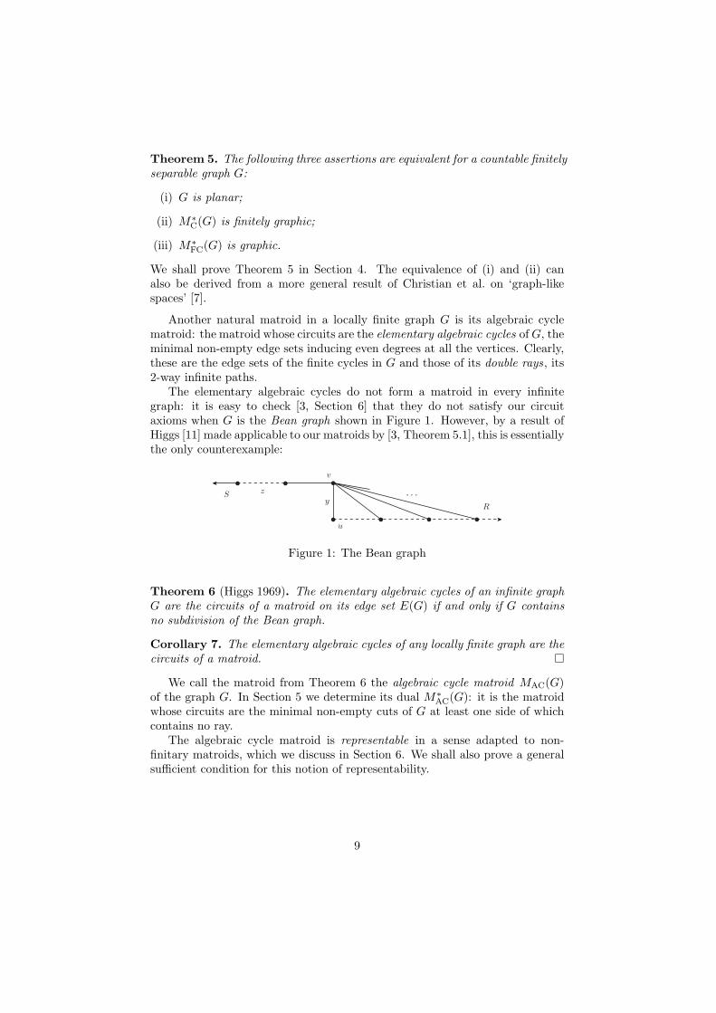
The elementary algebraic cycles do not form a matroid in every infinitegraph: it is easy to check [3, Section 6] that they do not satisfy our circuitaxioms when G is the Bean graph shown in Figure 1. However, by a result ofHiggs [11] made applicable to our matroids by [3, Theorem 5.1], this is essentiallythe only counterexample:

S z

v

u

yR

Figure 1: The Bean graph

Theorem 6 (Higgs 1969). The elementary algebraic cycles of an infinite graphG are the circuits of a matroid on its edge set E(G) if and only if G containsno subdivision of the Bean graph.

Corollary 7. The elementary algebraic cycles of any locally finite graph are thecircuits of a matroid.

We call the matroid from Theorem 6 the algebraic cycle matroid MAC(G)of the graph G. In Section 5 we determine its dual M⇤

AC(G): it is the matroidwhose circuits are the minimal non-empty cuts of G at least one side of whichcontains no ray.

The algebraic cycle matroid is representable in a sense adapted to non-finitary matroids, which we discuss in Section 6. We shall also prove a generalsu�cient condition for this notion of representability.

9

4 Proofs of Theorems 1, 2 and 5

We begin with the easy proof of Theorem 1, which we restate:

Theorem 1. Let G be any graph.

(i) The bonds of G, finite or infinite, are the circuits of a matroid MB(G),the bond matroid of G.

(ii) The bond matroid of G is the dual of its finite-cycle matroid MFC(G).

Proof. For simplicity we assume that G is connected; the general case is verysimilar. From [3] we know that MFC(G) has a dual; let us call this dual MB(G),and show that its circuits are the bonds of G. By definition of matroid duality,the circuits of MB(G) are the minimal edges sets that meet every spanning treeof G.

We show first that every bond B of G is a circuit of MB(G), a minimal setof edges meeting every spanning tree. Since B is a non-empty cut, it is the setof edges across some partition of the vertex set of G. Every spanning tree meetsboth sides of this partition, so it has an edge in B. On the other hand, we canextend any edge e 2 B to a spanning tree of G that contains no further from B,since by the minimality of B as a cut its two sides are connected in G. HenceB is minimal with the property of meeting every spanning tree.

Conversely, let B be any set of edges that is minimal with the propertyof meeting every spanning tree. We show that B contains a bond; by theimplication already shown, and its minimality, it will then be that bond. SinceG has a spanning tree, we have B 6= ;; let e 2 B. If B contains no bond, thenevery bond has an edge not in B. The subgraph H formed by all these edges isconnected and spanning in G, as otherwise the edges of G from the componentC of H containing e to any fixed component of G�C would form a bond of Gwith no edge in H, contradicting its definition. So H contains a spanning tree.This misses B, contradicting the choice of B.

We prove Theorem 2 for countable graphs; the proof for arbitrary graphs canbe deduced from this by considering a quotient space of kGk as explained in [16].For the remainder of this section, let G be a fixed countable connected graph.

We shall call two points in kGk (topologically) indistinguishable if they havethe same open neighbourhoods. Clearly two vertices or edge-ends x, y 2 kGkare indistinguishable if they cannot be separated by finitely many edges. (Ifboth are edge-ends, then x = y.) On the other hand, two such points that canbe separated by finitely many edges have disjoint open neighbourhoods. Innerpoints of edges are always distinguishable from all other points.

We shall need a few lemmas. Some of these are quoted from Schulz [16];the others are adaptations of results proved in [10] for the special case that Gis finitely separable. We remark that it is also possible to reduce Theorem 2formally to that case by replacing G with a quotient graph as explained in [16].

Lemma 8. [16] kGk is a compact space.

10

Lemma 9. Let X ✓ kGk be a closed subspace, with disjoint open subsets O1, O2

such that X = O1 [O2. Then the set F of edges of G with one endvertex in O1

and the other in O2 is finite.

Proof. Suppose F is infinite. As kGk is compact, the mid-points of the edgesin F have an accumulation point x in kGk. By definition of kGk, every neigh-bourhood of x contains infinitely many edges from F , and hence meets both O1

and O2. Since O1 and O2 are closed in X, and hence in kGk, this means thatx 2 O1 \O2, contradicting our assumption that O1 \O2 = ;.

In a Hausdor↵ space, every topological x–y path contains an injective suchpath, an x–y arc. Since kGk is not necessarily Hausdor↵ we cannot assume thisshortcut lemma in general, but it holds in the relevant case:

Lemma 10. [16] If two points x, y 2 V (G)[ E(G) are separated by a finite setof edges, then every topological x–y path contains an x–y arc.

Lemma 11. [16] Let x, y 2 V (G) [ E(G), and let (A�)�<� be a transfinitesequence of x–y arcs in kGk. Then there exists a topological x–y path P and adense subset P ⇤ of P so that for all p 2 P ⇤ the arcs A� containing p form acofinal subsequence.

Lemma 12. Every closed connected subspace X of kGk is path-connected.

Proof. Suppose X is connected but not path-connected. Then there are x, y 2V (G) [ E(G) contained in di↵erent path-components. In particular, x and yare topologically distinguishable, so they are separated by finitely many edges.Let e1, e2, . . . be a (possibly finite) enumeration of the edges in E(G) r E(X),let Fi := {e1, . . . , ei} for all i. If there exists an i such that x and y lie in theclosures of di↵erent graph-theoretical components of G � Fi, then picking aninner point outside X from every edge in Fi we obtain a finite set Z ✓ kGkrXwitnessing that x and y lie in distinct open sets of X whose union is all of X,contradicting our assumption that X is connected.

Hence for every i the points x and y lie in the closure Ci of the same com-ponent Ci of G� Fi. So for each i there is a path, ray or double ray connectingx to y in Ci, and with Lemma 10 we then obtain an x–y arc Ai in Ci. ByLemma 11 this implies that there is a topological x–y path P and a dense sub-set P ⇤ ✓ P such that for every p 2 P ⇤ the arcs Ai containing p form a cofinalsubsequence. Suppose there exists a j such that ej ✓ P . Then there must bea point p 2 ej \ P ⇤. However, none of the Ai with i � j contains ej . Thus, Pdoes not use any edge outside X. As X is closed, this implies that P ✓ X. Therequired x–y arc in X can be found inside P by Lemma 10.

Lemma 13. Let F ✓ E(G) be a set of edges whose closure in kGk contains nocircle. Then G has a topological spanning tree whose edge set contains F .

Proof. Let G = (V,E), let e1, e2, . . . be an enumeration of the edges in E r F ,and set T0 := E. Inductively, if the closure of (V, Ti�1� ei) is connected in kGkthen set Ti := Ti�1� ei; otherwise put Ti := Ti�1. Finally, we set T :=

T1i=0 Ti.

11

In order to show that T is the edge set of a topological spanning tree, letus first check that the closure X of (V, T ) is connected. Suppose there are twodisjoint non-empty open sets O1 and O2 of X with X = O1[O2. Then Lemma 9implies that the cut S consisting of the edges with one endvertex in O1 and theother in O2 is finite. If j is the largest integer with ej 2 S then, however, theclosure of (V, Tj) is not connected, a contradiction. Thus, T = X is connectedand therefore spanning. Moreover, T is path-connected, by Lemma 12.

Secondly, we need to show that T is acirclic. So, suppose that T contains acircle C. Since every circle lies in the closure of its edges but the closure of

SF

contains no circle, E(C)rF is non-empty. Pick j minimal with ej 2 E(C)rF .Since ej was not deleted from Tj�1 when Tj was formed, the closure Y of(V, Tj�1�ej) is disconnected. So there are two disjoint non-empty open subsetsO1, O2 of Y such that Y = O1 [ O2. The endvertices of ej do not lie in thesame Oi, since adding ej to that Oi would then yield a similar decomposition ofthe closure of (V, Tj�1), contradicting its connectedness. But now the connectedsubset C r ej of Y meets both O1 and O2, a contradiction. Thus, T does notcontain any circle and is therefore a topological spanning tree.

Lemma 14. Let C1 and C2 be two circles in kGk. Then E(C2) ✓ E(C1) impliesthat E(C1) = E(C2).

Proof. We first prove the following:

For every point x 2 C1 r C1 there is a point y 2 C1 such that xand y are indistinguishable.

(1)

Indeed, consider a z 2 kGk that is distinguishable from all points in C1. Thus,we may pick for every p 2 C1 two disjoint open neighbourhoods Op

z and Op of zand p, respectively. Note that C1 is compact, being a continuous image of thecompact space S1. Thus, there is a finite subcover Op1 [ . . .[Opn of C1. Then,the open set \n

i=1Opiz is disjoint from C1 and contains z. Hence, z does not lie

in the closure of C1. This proves (1).Next, suppose that E(C2) is a proper subset of E(C1), and pick e 2 E(C2)

and f 2 E(C1) r E(C2). Since X := C1 r (e [ f) is disconnected there existtwo disjoint non-empty open sets O0

1 and O02 of X with X = O0

1 [ O02. For

j = 1, 2, denote by Ij the set of points x in kGk for which there is a y 2 O0j

such that x and y are indistinguishable. Then O1 := O01 [ I1 and O2 := O0

2 [ I2

are disjoint and open subsets of X [ I1 [ I2. Moreover, it follows from (1) thatC1 r (e [ f) = X [ I1 [ I2. Therefore, O1 and O2 are two disjoint non-emptyopen sets of C1 r (e [ f) with C1 r (e [ f) = O1 [O2.

As C2 r e is a connected subset of C1 r (e [ f) it lies in O1 or in O2, letus say in O1. Then O1 := O1 [ e and O2 are two disjoint non-empty opensubsets of C1 r f with C1 r f = O1 [O2. By (1), this means that also C1 r fis disconnected. But C1 r f is a continuous image of a connected space, andhence connected.

12

Lemma 15. Let T be a standard subspace of kGk. Then the following state-ments are equivalent:

(i) T is a topological spanning tree of kGk.

(ii) T is maximally acirclic, that is, it does not contain a circle but adding anyedge in E(G) r E(T ) creates one.

(iii) E(T ) meets every finite bond, and is minimal with this property.

Proof. Let us first prove a part of (iii)!(i) before dealing with all the otherimplications.

If E(T ) meets every finite bond then T is spanning and path-connected.

(2)

Suppose that the closure X of (V (G), E(T )) is not connected. Then there aretwo disjoint non-empty open sets O1 and O2 of X with X = O1 [ O2. FromLemma 9 we get that the cut consisting of the edges with one endvertex inO1 and the other in O2 is finite. Since each of O1 and O2 needs to contain avertex, this cut is non-empty. Hence, E(T ) misses a finite bond, a contradiction.Therefore, T = X is connected and then, by Lemma 12, path-connected.

(i) ! (ii) Consider any edge e /2 E(G) r E(T ). If the endvertices u and vof e cannot be separated by finitely many edges then e � u (and also e � v) isa circle in kGk. Otherwise, any topological u–v path contains an u–v arc byLemma 10. In particular, T contains an u–v arc that together with e forms acircle.

(ii) ! (iii) Suppose that E(T ) misses a finite bond F . Pick e 2 F , and letC be a circle in T [ e through e. Pick an inner point of every edge in F anddenote the set of these points by Z. Then the two components of kGkrZ, eachof which contains an endvertex of e, form two disjoint open sets containing T .However, C r e ✓ T is a connected set that meets both of these disjoint opensets, which is impossible. Thus, E(T ) meets every finite bond. In particular, Tis spanning and path-connected, by (2).

Let f be any edge in E(T ), and let us show that E(T )�f misses some finitebond. Denote the endvertices of f by r and s, and observe that r and s canbe separated by finitely many edges as T is acirclic. Denote by Kr and Ks thepath-components of T r f containing r and s, respectively. By Lemma 10 andas T does not contain any circle, Kr and Ks are distinct, and thus disjoint. AsT is path-connected, it follows that T r f is the disjoint union of the open setsKr and Ks. Now Lemma 9 yields that there are only finitely many edges withone endvertex in Kr and the other in Ks. As T is spanning this means thatE(T )� f misses a finite cut.

(iii) ! (i) By (2), we only need to check that T does not contain any circle.Suppose there exists a circle C ✓ T , and pick some e 2 E(C). By the minimalityof E(T ) there exists a finite bond F so that F is disjoint from T r e. Then,however, picking inner points from the edges in F yields a set Z, so that theconnected set C r e is contained in kGk r Z but meets two components ofkGkr Z, which is impossible.

13

We can now prove our main theorem, which we restate:

Theorem 2.

(i) The edge sets of the circles in kGk are the circuits of a matroid MC(G),the cycle matroid of G.

(ii) The bases of MC(G) are the edge sets of the topological spanning trees of G.

(iii) The cycle matroid MC(G) is the dual of the finite-bond matroid MFB(G).

Proof. To bypass the need to verify any matroid axioms, we define MC(G) asthe dual of MFB(G) (which we know exists [3]), ie., as the matroid whose basesB are the complements of the bases of MFB(G). These latter are the maximaledge sets not containing a finite bond, so the bases B of MC(G) are the minimaledge sets meeting every finite bond. By Lemma 15 below, this is equivalent toB being the edge set of a topological spanning tree of kGk.

We have defined MC(G) so as to make (iii) true, and shown (ii). It remainsto show (i): that the circuits of MC(G) are the edge sets of the circles in kGk.Since no circuit of a matroid contains another circuit, and since by Lemma 14no edge set of a circle contains another such set, it su�ces to show that everycircuit contains the edge set of a circle, and conversely every edge set of a circlecontains a circuit.

For the first of these statements note that, by assertion (ii), a circuit Dof MC(G) does not extend to the edge set of a topological spanning tree. Henceby Lemma 13 its closure

SD in kGk contains a circle C. For the second state-

ment, note that the edge set D of a circle C is not contained in the edge set ofa topological spanning tree T , because T is closed and would therefore containS

D ◆ C, contradicting its definition. Hence D is dependent in MC(G), andtherefore contains a circuit [3].

Finally, let us restate and prove Theorem 5:

Theorem 5. The following three assertions are equivalent for a countable finitelyseparable graph G:

(i) G is planar;

(ii) M⇤C(G) is finitely graphic;

(iii) M⇤FC(G) is graphic.

Proof. If G is planar, it has a dual G⇤. Then M⇤C(G) = MFC(G⇤) by Theorem 4,

and M⇤FC(G) = MB(G) = MC(G⇤) by Theorems 1 and 3 (ii).

(ii)!(i): Since M⇤C(G) is finitely graphic, there exists a graph H with the

same edge set as G such that M⇤C(G) = MFC(H). As M⇤

FC(H) = MB(H) byTheorem 1 and matroid duals are unique, we obtain MC(G) = MB(H). Hencethe edge sets of the circles in kGk, which by Theorem 2 (i) are the circuits

14

of MC(G), are precisely the bonds of H. So H is a dual of G, and G is planarby Theorem 3 (i).

(iii)!(i): Let H be a graph such that MC(H) = M⇤FC(G). To show that

G is planar, it su�ces by Kuratowski’s theorem10 to check that G has no K5-or K3,3-minor, or in matroid terms, that MFC(G) has no minor isomorphic toMC(K5) or MC(K3,3). As M⇤

FC(G) = MC(H), this is equivalent to saying thatMC(H) has no M⇤

C(K5) or M⇤C(K3,3)-minor. These latter two matroids are not

graphic [14, Prop. 2.3.3], so it thus su�ces to show that the finite minors ofMC(H) are graphic.

To prove this, consider a finite minor M of MC(H), obtained by deleting theset X ✓ E(H) and contracting the set Y ✓ E(H), say. Let V be the finite setof vertices of H incident with an edge in the ground set E of M , and let K bethe finite graph obtained from the graph (V,E) by identifying any two verticesthat are either indistinguishable in kHk or joined by an arc in kHk whose edgeslie in some fixed base B of the restriction of MC(H) to Y . Using Lemma 10 and[3, Lemma 3.5], it is now easy to show that M = MC(K). Hence M is graphic,as desired.

We remark that the graphs witnessing (ii) and (iii) in Theorem 5 can bechosen to be finitely separable, too. Indeed, the graph G⇤ which we used in ourproof as a witness for both (ii) and (iii) is finitely separable by Theorem 3 (ii).

5 The dual of the algebraic cycle matroid

Recall from Theorem 6 that the elementary algebraic cycles of a graph G arethe circuits of a matroid, the algebraic cycle matroid MAC(G) of G, if and onlyif G contains no subdivision of the graph shown in Figure 1. In this section wecharacterize its dual M⇤

AC(G).Recall that a ray is a 1-way infinite path. Let us call a non-empty cut

F = E(A,B) of G skew if one of its sides A,B is small in the sense that thesubgraph it induces in G contains no ray and F is minimal with this propertyamong the non-empty cuts of G. If G is connected then so is the small side ofany skew cut, so this will be finite if G is connected and locally finite.

Theorem 16. The cocircuits of a matroid M that is the algebraic cycle matroidof a graph G are precisely the skew cuts of G.

Casteels and Richter [6] studied a related duality: they showed that, in alocally finite graph, the cuts with a finite side form the orthogonal space of theset of elementary algebraic cycles.

For our proof of Theorem 16 we need the following easy lemma from [3]:

Lemma 17. A circuit and a cocircuit of a matroid never meet in exactly oneelement.

10Its extension to countable graphs is straightforward by compactness; see [9, Exercise 8.23].

15

Proof of Theorem 16. Let us show first that every non-empty cut F with a smallside A contains a cocircuit of M . If not, F is independent in M⇤, so it avoidsa base B of M . Adding an element f 2 F to B creates a circuit of M , a cycleor double ray that meets F precisely in f . Since G[A] contains no ray, this isimpossible.

Conversely, let us show that every cocircuit D of M contains a skew cut.Pick an edge e 2 D. If its endvertices lie in the same component of G � D,then G contains a cycle meeting D in exactly e, contradicting Lemma 17. Sothe endvertices of e lie in distinct components of G�D. If both these containa ray, then these rays can be chosen so as to combine with e to a double raymeeting D precisely in e, again contradicting Lemma 17. Hence one of thesecomponents contains no ray. Its vertex set A is the small side of a cut F withe 2 F ✓ D. To show that F is a skew cut, we still have to show that it containsno non-empty cut F 0 with a small side properly. But any such F 0 contains acocircuit D0, as shown earlier, giving D0 ✓ F 0 ( F ✓ D. This contradicts thefact that no cocircuit contains another cocircuit properly.

We have shown that every skew cut contains a cocircuit, and vice versa.Since skew cuts, as cocircuits, cannot contain each other properly, these inclu-sions cannot be proper. So the cocircuits of M are the skew cuts of G.

6 Thin-sum matroids and representability

In finite matroid theory, representable matroids are an important generalizationof graphic matroids. As matroids defined by linear independence are finitary,the dual of an infinite representable matroid will not, except in trivial cases, berepresentable. Representability, as usually defined, is thus another concept thatseems too narrow for infinite matroids.

In this section we present a notion of vector independence, di↵erent from lin-ear independence, that can give rise to non-finitary matroids. Examples includethe algebraic cycle matroids of graphs and of higher-dimensional complexes [3].

Let F be a field, and let A be some set. We say that a set X of functionsx : A ! F is thin if for every a 2 A there are only finitely many x 2 X withx(a) 6= 0. Given such a thin set of functions, their pointwise sum

Px2X x is

another A ! F function. We say that a set of A ! F functions, not necessarilythin,11 is thinly independent if for every thin subset X and every correspondingfamily (↵x)x2X of coe�cients ↵x 2 F we have

Px2X ↵xx = 0 2 FA only when

↵x = 0 for all x 2 X.Unlike linear independence, thin independence does not always define a ma-

troid.12 The following theorem gives a su�cient condition for when it does:11Requiring independent sets to be thin leads to a di↵erent notion of representability that

may have its own applications. It is easily seen that this notion does not satisfy (IM) forarbitrary sets E of A ! F functions, but there may be interesting examples where it does.

12View the elements of E = FN2 as subsets of N, and define sets I := {{1, n} : n 2 N} and

I0 := {{n} : n 2 N}. Both I and I0 are thinly independent. Moreover, I0 is maximally thinlyindependent but I is not: I + N, for instance, is still thinly independent. Yet, the only x 2 I0

for which I + x is thinly independent is x = {1}, which is already contained in I. Thus, (I3)

16

Theorem 18. If a set E of A ! F functions is thin, then its thinly independentsubsets form the independent sets of a matroid on E.

Let us call such a matroid as in Theorem 18 the thin-sums matroid of thefunctions in E. In the remainder of this section we prove Theorem 18, and thenbriefly discuss what it means for graphs.

Let F be endowed with the discrete topology, and the set FA of all A ! Ffunctions with the product topology. Thus for each x 2 FA, the sets

{ y 2 FA : y(a) = x(a) for all a 2 A0}

where A0 ranges over the finite subsets of A forms a basis of the open neigh-bourhoods of x.

Given a set X of functions A ! F , we write hXi for the set of all func-tions A ! F that are of the form

Px2X0 ↵xx, where X 0 ✓ X and X 0 is thin.

Similarly, we write X for the closure in FA of the set X.In contrast to [4] where these concepts were introduced, X will here always be

a subset of a thin set E. While the sets hXi and X may contain elements outsideour ground set E, we note that X 7! hXi \E is the closure operator associatedwith the set I of thinly independent subsets of E, as defined in Section 2.

We need two lemmas from [4], which together imply that hhXii = hXi forall our (thin) sets X ✓ E:

Lemma 19. [4, Lemma 5] Every thin set X ✓ FA satisfies hXi = hXi.Lemma 20. [4, Lemma 6] Every set X ✓ FA satisfies hhXii ✓ hXi.

Proof of Theorem 18. Let I be the set of thinly independent subsets of E.Clearly, I satisfies (I1) and (I2).13

Our first claim is that, for all sets J ✓ X ✓ E with J 2 I,

if X ✓ hJi then J is a maximal element of {I 2 I : I ✓ X}. (3)

Consider an x 2 X r J . Then there are coe�cients aj 2 F , j 2 J , such thatPj2J ajj = x. Thus, J + x is not thinly independent for any x 2 X r J , which

implies the claim.To prove that I satisfies (I3), let I 2 I r Imax and I 0 2 Imax be given. We

have to find an x 2 I 0 r I such that I + x is still thinly independent. Clearly,any x in I 0 r hIi will do, so it su�ces to show that I 0 6✓ hIi. If I 0 ✓ hIi, thenhI 0i ✓ hhIii = hIi by Lemmas 19 and 20. As I 0 2 Imax implies E ✓ hI 0i, thisyields E ✓ hI 0i ✓ hIi, which contradicts (3). This completes the proof of (I3).

is violated.13We use the independence axioms in our proof. Alternatively, one could check that h · i\E

is indeed the closure operator associated with I and then use the closure axioms: (CL1),(CL2) and (CL4) are straightforward, (CL3) follows from our two lemmas, and (CLM) isproved like (IM) in the text.

17

Next, we prove that I satisfies (IM). This will follow directly from (3) andthe following claim:

For all sets I ✓ X ✓ E with I 2 I, there is a B 2 I withI ✓ B ✓ X and X ✓ hBi. (4)

In the remainder of this proof we thus prove (4). Let x1, x2, . . . be a (possiblytransfinite) enumeration of X r I. Inductively, we define nested sets B� ✓ Xas follows. Start with B0 := I. If, in step �, there are families (↵µ)µ>� and(�i)i2I of coe�cients in F such that

x� =Xµ>�

↵µxµ +Xi2I

�ii

(these sums are well-defined, since E is thin by assumption), we set B� :=Sµ<� Bµ. Otherwise we put B� := {x�}[

Sµ<� Bµ. Finally, we let B :=

S� B�,

which we claim satisfies (4).Let us first check that B 2 I. If not then there are coe�cients ↵b 2 F

for all b 2 B, not all of them zero, such thatP

b2B ↵bb = 0. Since I is thinlyindependent, there must be some b 2 B r I with ↵b 6= 0. Pick such a functionb = x� with smallest index �. Then

�x� =X

x2{xµ:µ>�}\B

↵�1x�

↵xx +Xi2I

↵�1x�

↵ii ,

which contradicts the fact that x� 2 B.Next, we prove X ✓ hBi. By Lemma 19 this will imply X ✓ hBi = hBi,

which then completes the proof of (4).To prove X ✓ hBi, consider a function z 2 X. We need to find, for every

finite subset A0 of A, a function z0 2 hBi that agrees with z on A0. Denote byL the set of x 2 X for which there is an a 2 A0 with x(a) 6= 0. Observe that Lis a finite set, since A0 is finite and X ✓ E is thin. In particular, we may writeL r B = {x�1 , . . . , x�k}, where �1 < . . . < �k. Let ` be the largest numberin {1, . . . , k + 1} for which there exists a y 2 h{x�` , . . . , x�k} [ (B \ L)i withy(a) = z(a) for all a 2 A0. Note that there is always such a y for ` = 1, as wemay either pick y = z if z 2 L, or y = 0 otherwise. Note, furthermore, that wehave found the desired z0 if ` = k + 1, as then z0 := y 2 hBi.

Suppose that ` k. Since x�` /2 B there are coe�cients (↵µ)µ>�` and(�i)i2I such that x�` =

Pµ>�`

↵µxµ +P

i2I �ii. Then

x�` =X

µ>�`, xµ /2B

↵µxµ +Xb2B

�0bb

with suitable coe�cients �0b. Restricting this to L, set

r :=kX

p=`+1

↵�px�p +X

b2B\L

�0bb .

18

Then

r(a) = x�`(a) for all a 2 A0, and r 2 h{x�`+1 , . . . , x�k} [ (B \ L)i.

Next, by choice of ` there exists y =Pk

q=` ��qx�q +P

b2B\L �bb such thaty(a) = z(a) for all a 2 A0. Replacing x�` in this sum with r, we obtain

y⇤ := ��`r +kX

q=`+1

��qx�q +X

b2B\L

�bb 2 h{x�`+1 , . . . , x�k} [ (B \ L)i.

As y⇤ agrees with z on A0, this contradicts the maximal choice of `.

The algebraic cycle matroid of a graph G = (V,E) can be represented as athin-sums matroid over F2, for any G for which it is defined (cf. Theorem 6).Indeed, as in finite graphs we represent an edge e = uv by the map V ! F2

assigning 1 to both u and v, and 0 to every other vertex. Then a set F ✓ E ofedges becomes a set of V ! F2 functions, not necessarily thin, which is thinlyindependent if and only if F contains no elementary algebraic cycle. This exam-ple can be generalized to higher dimensions; see [3] for algebraic cycle matroidsof simplicial complexes.

We do not know whether the other non-finitary matroids we discussed inthis paper are representable as thin-sum matroids, but suspect not. For fini-tary matroids, one would hope that ‘thin-sum’ representability coincides withtraditional representability, but we have no proof of this:

Problem 21. Is a finitary matroid representable as a thin-sums matroid if andonly if it is representable in the usual sense?

We can show that the finite-cycle matroid MFC(G) of a graph G is a thin-sums matroid if G has finite chromatic number, but we do not know this forarbitrary G.

Acknowledgement

We would like to thank Robin Christian for indicating the proof of implication(iii)!(i) of Theorem 5, which we had previously stated as a conjecture.

References

[1] D.W.T. Bean, A connected finitary co-finitary matroid is finite, Proceedingsof the Seventh Southeastern Conference on Combinatorics, Graph Theoryand Computing, Congressus Numerantium, vol. 17, 1976, pp. 115–19.

[2] H. Bruhn and R. Diestel, Duality in infinite graphs, Comb., Probab.Comput. 15 (2006), 75–90.

19

[3] H. Bruhn, R. Diestel, M. Kriesell, R. Pendavingh, and P. Wollan, Axiomsfor infinite matroids, arXiv:1003.3919 (2010).

[4] H. Bruhn and A. Georgakopoulos, Bases and closures under infinite sums,Linear Algebra and its Applications 435 (2011), 2007–2018.

[5] H. Bruhn and P. Wollan, Finite connectivity in infinite matroids,J. Combin. Theory (Series B) (to appear).

[6] K. Casteels and B. Richter, The Bond and Cycle Spaces of an InfiniteGraph, J. Graph Theory 59 (2008), no. 2, 162–176.

[7] R. Christian, R.B. Richter, and B. Rooney, The planarity theorems ofMacLane and Whitney for graph-like continua, Electronic J. Comb. 17(2009), #R12.

[8] R. Diestel, Locally finite graphs with ends: a topological approach,http://arxiv.org/abs/0912.4213, 2009.

[9] , Graph Theory, 4th ed., Springer, 2010.

[10] R. Diestel and D. Kuhn, Topological paths, cycles and spanning trees ininfinite graphs, Europ. J. Combinatorics 25 (2004), 835–862.

[11] D.A. Higgs, Infinite graphs and matroids, Recent Progress in Combi-natorics, Proceedings Third Waterloo Conference on Combinatorics,Academic Press, 1969, pp. 245–53.

[12] , Matroids and duality, Colloq. Math. 20 (1969), 215–220.

[13] J.G. Oxley, Infinite matroids, Matroid applications (N. White, ed.), Encycl.Math. Appl., vol. 40, Cambridge University Press, 1992, pp. 73–90.

[14] , Matroid theory, Oxford University Press, 1992.

[15] R. Rado, Abstract linear dependence, Colloq. Math. 14 (1966), 257–64.

[16] M. Schulz, Der Zyklenraum nicht lokal-endlicher Graphen, DiplomarbeitUniversitat Hamburg 2005, http://www.math.uni-hamburg.de/home/diestel/papers/others/Schulz.Diplomarbeit.pdf.

[17] M. Stein, Extremal infinite graph theory, Discrete Math. 311 (2011),1472–1496.

[18] C. Thomassen, Duality of infinite graphs, J. Combin. Theory (Series B)33 (1982), 137–160.

[19] M. Las Vergnas, Sur la dualite en theorie des matroıdes, Theorie desMatroıdes, Lecture notes in mathematics, vol. 211, Springer-Verlag, 1971,pp. 67–85.

Version 12 March 2011.Footnotes 5 and 6 were added later. Figure 1 was corrected in May 2012.

20