Received: 17 July 2017 Accepted: 2 November 2017

DO

I: 10.1002/hyp.11399

R E S E A R CH AR T I C L E

Infiltration into frozen soil: From core‐scale dynamicsto hillslope‐scale connectivity

Willemijn M. Appels | Anna E. Coles | Jeffrey J. McDonnell

Global Institute for Water Security & School of

Environment and Sustainability, University of

Saskatchewan, 11 Innovation Boulevard,

Saskatoon, SK S7N 3H5, Canada

Correspondence

Willemijn M. Appels, Lethbridge College,

3000 College Drive S, Lethbridge,

AB T1K 1L6, Canada.

Email: willemijn.appels@gmail.com

Present Address

A. E. Coles, Wilfrid Laurier University, 5007 50

Avenue, Yellowknife, NT X1A 2P8, Canada.

66 Copyright © 2017 John Wiley & Sons, Lt

Abstract

Infiltration into frozen soil is a key hydrological process in cold regions. Although the mechanisms

behind point‐scale infiltration into frozen soil are relatively well understood, questions remain

about upscaling point‐scale results to estimate hillslope‐scale run‐off generation. Here, we tackle

this question by combining laboratory, field, and modelling experiments. Six large (0.30‐m diam-

eter by 0.35‐m deep) soil cores were extracted from an experimental hillslope on the Canadian

Prairies. In the laboratory, we measured run‐off and infiltration rates of the cores for two ante-

cedent moisture conditions under snowmelt rates and diurnal freeze–thaw conditions observed

on the same hillslope. We combined the infiltration data with spatially variable data from the

hillslope, to parameterise a surface run‐off redistribution model. We used the model to determine

how spatial patterns of soil water content, snowpack water equivalent (SWE), and snowmelt rates

affect the spatial variability of infiltration and hydrological connectivity over frozen soil. Our

experiments showed that antecedent moisture conditions of the frozen soil affected infiltration

rates by limiting the initial soil storage capacity and infiltration front penetration depth. However,

shallow depths of infiltration and refreezing created saturated conditions at the surface for dry

and wet antecedent conditions, resulting in similar final infiltration rates (0.3 mm hr−1). On the

hillslope‐scale, the spatial variability of snowmelt rates controlled the development of hydrolog-

ical connectivity during the 2014 spring melt, whereas SWE and antecedent soil moisture were

unimportant. Geostatistical analysis showed that this was because SWE variability and anteced-

ent moisture variability occurred at distances shorter than that of topographic variability, whereas

melt variability occurred at distances longer than that of topographic variability. The importance

of spatial controls will shift for differing locations and winter conditions. Overall, our results

suggest that run‐off connectivity is determined by (a) a pre‐fill phase, during which a thin surface

soil layer wets up, refreezes, and saturates, before infiltration excess run‐off is generated and (b) a

subsequent fill‐and‐spill phase on the surface that drives hillslope‐scale run‐off.

KEYWORDS

hydrological connectivity, infiltration into frozen ground, spatial variability of snowpack, spring

snowmelt

1 | INTRODUCTION

Infiltration into frozen soil is an important hydrological flux in cold

regions (Fang & Pomeroy, 2007; Ireson, van der Kamp, Ferguson,

Nachson, & Wheater, 2013). In these regions, spring snowmelt is typ-

ically the dominant hydrological event of the year. On the Canadian

Prairies, where frozen ground persists through the melt season, snow-

melt drives up to 80% of annual run‐off. The partitioning of snowmelt

between infiltration into frozen soils and run‐off determines flooding

d. wileyonlinelib

(Gray, Landine, & Granger, 1985; Kane & Stein, 1984; Li & Simonovic,

2002), soil moisture variability and availability for crop production

(Gray, Norum, & Granger, 1984; McConkey, Ulrich, & Dyck, 1997),

and solute transport (Su et al., 2011). Understanding infiltration into

frozen soil is therefore crucial for predicting these water resource

issues.

Gravity and capillary forces drive infiltration into frozen soil. Cap-

illary processes are more complex in frozen than in unfrozen soils due

to coupled energy and mass transfer associated with phase changes

Hydrological Processes. 2018;32:66–79.rary.com/journal/hyp

APPELS ET AL. 67

(Kane & Stein, 1983). A frozen soil is a continuum of particles: large

air‐filled pores, intermediate ice‐filled pores, small liquid water‐filled

pores, and liquid water films around particles (Stähli, Jansson, & Lundin,

1999). The extent to which pores are filled with air, ice, and water are

determined by soil water content before freeze‐up and pore size

distribution (Watanabe & Wake, 2009). Ice‐filled pores decrease the

total pore space and increase the tortuosity of the remaining pore

space, resulting in a lower hydraulic conductivity of the remaining pore

domain and consequently reduced infiltration rates compared to

unfrozen soils (Stähli et al., 1999). The soil water content before

freeze‐up is therefore a key variable in empirical frozen soil infiltration

equations (Granger, Gray, & Dyck, 1984; Zhao & Gray, 1997). Heat

transport affects infiltration rates into frozen soils more than those

into unfrozen soils. When soils remain frozen during the melt period,

infiltrated water refreezes in the infiltration zone, limiting rates even

further (Stähli et al., 1999), whereas soil thaw during the infiltration

period is accompanied by sudden jumps in infiltration rates (Hayashi,

van der Kamp, & Schmidt, 2003; Watanabe et al., 2012).

Despite having identified most of the physical aspects of the infil-

tration into frozen soil process—amassed from a plethora of laboratory

(e.g., Lilbæk & Pomeroy, 2010; McCauley, White, Lilly, & Nyman, 2002;

Watanabe et al., 2012), field (e.g., Bayard, Stähli, Parriaux, & Flühler,

2005; Granger et al., 1984; Hayashi et al., 2003; Iwata, Hayashi,

Suzuki, Hirota, & Hasegawa, 2010; Kane & Stein, 1983, 1984), and

modelling studies (e.g., Gray et al., 1985; Gray, Toth, Zhao, Pomeroy,

& Granger, 2001; Hansson, Šimůnek, Mizoguchi, Lundin, & van

Genuchten, 2004; Jansson & Karlberg, 2001; Kane, Hinkel, Goering,

Hinzman, & Outcalt, 2001; Kitterød, 2008; Ling & Zhang, 2004;

Motovilov, 1978, 1979; Painter, 2011; Romanovsky & Osterkamp,

2000; Zhao & Gray, 1997; Zhao, Gray, & Male, 1997)—we still struggle

to apply our point‐scale understanding to the hillslope‐ and catchment‐

scales. This has implications for our ability to predict run‐off genera-

tion, soil moisture conditions, and solute transport occurring at those

larger scales.

The scaling difficulties lie partly in the presence of environmental

factors, for example, wind‐driven snow redistribution, land‐use‐driven

accumulation, and soil insulation, which may affect melt, thaw, and

thereby the infiltration process itself (Hayashi, 2013). They can also

be attributed to the design of laboratory studies, in which the use of

repacked (as opposed to intact) soil columns and a focus on ponded

water conditions are typical (Hansson et al., 2004; Lilbæk & Pomeroy,

2010; McCauley et al., 2002; Moghadas, Gustafsson, Viklander,

Marsalek, & Viklander, 2016; Watanabe et al., 2012). With the notable

exception of the study of Watanabe and Kugisaki (2017), who con-

ducted one‐dimensional column experiments with macroporous soils,

these typical laboratory studies cannot be easily scaled to understand

field conditions where macropore flow and nonponded infiltration

may dominate (Ishikawa, Zhang, Kadota, & Ohata, 2006; Stähli,

Jansson, & Lundin, 1996). But infiltration into frozen soil is also very

difficult to measure directly in the field (Baker, 2006) because of

instrument error in sub‐zero conditions and the effects of an overlying

snowpack. As a result, in the field, hillslope‐averaged melt into frozen

soil is usually deduced from snowpack and run‐off observations, which

unfortunately reveal little about the spatial variability in infiltration or

soil water content. Finally, a paucity of reliable data and the

complexities associated with solving the coupled energy and water

balance mean infiltration into frozen soil is notoriously difficult to

validate with hydrological models (Gupta & Sorooshian, 1997;

Pomeroy et al., 2007).

So what can be done? It is imperative that we bridge the gap

between core‐scale and hillslope‐scale understanding of infiltration

into frozen soil. Here, we tackle this research challenge with a com-

bined laboratory, field, and modelling experiment. We undertook labo-

ratory experiments on large, intact soil cores extracted from a 5 ha

experimental hillslope on the Canadian Prairies. The laboratory exper-

iments simulated nonponding snowmelt conditions during a multiday

event, where the soil water content, air temperature and snowmelt

rates were driven with observed data from a field season in spring

2014 at the same 5 ha experimental hillslope (Coles & McDonnell,

2017). We then combined the laboratory‐generated, core‐scale infil-

tration data, with spatially variable hillslope‐scale data observed during

the 2014 field season, to parameterise a surface run‐off redistribution

model. We used that model to determine how the spatial patterns of

the hydrological variables relevant during spring melt affects the spa-

tial variability of infiltration into frozen soil and run‐off generation at

the hillslope‐scale.

Overall, our novel core‐ to hillslope‐scales study of infiltration into

frozen soil sought to answer the following questions:

1. What is the relationship between soil water content at freeze‐up

and core‐scale infiltration and run‐off rates during snowmelt?

2. How does this relationship affect the spatial variability of infiltra-

tion‐run‐off partitioning at the hillslope‐scale?

3. To what extent does the spatial variability of hydrological vari-

ables (soil water content at freeze‐up, snowpack snow water

equivalent [SWE], and snowmelt rate) influence hillslope‐scale

infiltration‐run‐off patterns?

2 | METHODS

2.1 | Soil core extraction and instrumentation

We extracted six undisturbed soil cores from a hillslope at the Swift

Current Research and Development Centre in Swift Current (SK,

Canada) in June 2014. This is one of three experimental hillslopes in

the 1962–2013 run‐off, precipitation, and soil water content monitor-

ing programme of Agriculture andAgri‐FoodCanada (Coles,McConkey,

&McDonnell, 2017) and the location of the hillslope‐scale observations

described below (Coles & McDonnell, 2017). We constructed a stain-

less steel corer to extract six 0.30 m in diameter by 0.35 m high intact

soil cores. The corer approach followed Tindall, Hemmen, and Dowd

(1992) with a vertical disarticulating spring‐apart seam to enable the soil

core to be removed intact from the corer. We used a hydraulic press to

push the corer into the ground and then used hand shovels to carefully

excavate the earth from around the outsides of the buried corer, and lift

it from the ground. We removed the stainless‐steel corer and wrapped

the soil core in flexible sheet metal (5 × 10−4 m thick, 0.40 m high, and

1.05 m wide) to form a cylinder 0.40 m high around the soil core. The

68 APPELS ET AL.

top of the cylinder was 0.05 m above the surface of the soil core. The

base of the soil core was loosely wrapped in a coarse mesh fabric that

allowedwater to freely drain from the bottomof the core but prevented

chunks of soil from breaking off the cores. The sheet metal and mesh

fabric were held in place with hose clamps.

We drilled through the metal casing at pre‐determined depths in

order to instrument the soil cores to monitor soil water content and

temperature. The soil cores were instrumented with four Stevens

HydraProbe II soil water content sensors at depths of: 0.05 m (2),

0.15 m (1), and 0.25 m (1) for volumetric water content—θTOP, θMID,

and θBASE, respectively (Figure 1). We also installed 19 thermocou-

ples (Type T Copper/Constantan) at increments of 0.01 m over

depths of 0.01–0.10 m and increments of 0.02 m over depths of

0.12–0.28 m, to measure temperature through the soil core

(Figure 1). Soil water content and temperature data were logged at

30‐s intervals.

The cores were wrapped in insulating material, maintaining frozen

conditions in the body of the cores, as the air temperature of the

freezer was increased. The top and bottom of the cores were directly

exposed to the air temperature of the freezer. The tops were more

exposed to airflow than the bottom, due to the very small space

between the bottom of the cores and the lab bench on which they

were placed. Upward soil thaw at the bottoms of the cores could

occur, especially at low initial moisture content. At the beginning of

the experiment, we anticipated that the penetration of such a thaw

front would not be large enough to affect the infiltration front. This

assumption was checked with temperature data from lower depths in

the cores.

2.2 | Core‐scale simulated snowmelt events

We conducted two simulated snowmelt event experiments, with three

replicate cores for each event. The experiments were differentiated by

their antecedent soil moisture conditions: dry (0.11 m3 m−3) and wet

(0.18 m3 m−3). We dried down or wetted up the cores to the desired

start conditions, after which we froze the cores in a walk‐in freezer.

We sloped the surface of the soil cores at an angle of 5% to collect

surface run‐off. Each experiment was 4 days in duration with diurnal

freezing and thawing, where we varied the air temperature of the

freezer between −5 and +2°C according to measured diurnal tempera-

ture conditions in the field. We applied 50 mm of “snowmelt” water

directly to the surface of the soil cores using a plant sprayer, with rates

varying between 0 and 160 mm d−1. This represented snowmelt rates

observed during the main melt period of the 2014 snowmelt season at

the Swift Current site as described by Coles and McDonnell (2017).

The air temperature fluctuations and snowmelt applications were car-

ried out in real time (i.e., 1 hr of experiment = 1 hr of observed data

from the field). The temperature of the “snowmelt” water was main-

tained at 0–1 °C by keeping ice in the water buckets. We added

brilliant blue dye to the “snowmelt” water applied to one core in the

dry experiment. After that experiment, we dissected the dyed core

by cutting vertical and horizontal sections for qualitative analysis of

infiltration patterns and any preferential flow pathways, following

methods of Flury, Flühler, Jury, and Leuenberger (1994) and Weiler

and Flühler (2004).

Any surface run‐off during the experiments was routed through a

hole in the core's metal casing at the downslope end of the core and

collected in a small bucket. We recorded run‐off volumes (mL) on an

hourly basis and converted these to run‐off rates (mm hr−1). We used

the snowmelt and run‐off rates to determine infiltration rates and infil-

tration capacities of the soil. Instead of using a dedicated infiltration

equation for frozen soils, we used the format of Philip's infiltration

equation originally derived for unfrozen soils (Philip, 1957a). The fol-

lowing equation was fitted to the observed time series of infiltration

rate on the days that run‐off was generated:

IC ¼ Sa2

ffiffit

p þ Ke; (1)

where IC is infiltration capacity (m d−1), Sa is the apparent sorptivity

(m d−1/2), t is time (d), and Ke is the final infiltration capacity or effective

saturated hydraulic conductivity of the frozen soil (m d−1). In the orig-

inal Philip infiltration equation, sorptivity is a measure of the ability of

soil to absorb liquid by capillarity, affected by soil texture and initial

FIGURE 1 Dimensions and instrumentationof the experimental soil cores in side view andplan view

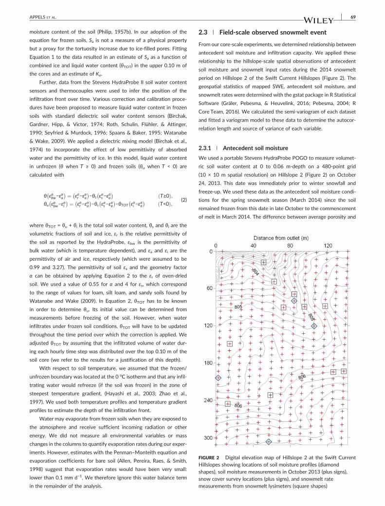
FIGURE 2 Digital elevation map of Hillslope 2 at the Swift CurrentHillslopes showing locations of soil moisture profiles (diamondshapes), soil moisture measurements in October 2013 (plus signs),snow cover survey locations (plus signs), and snowmelt ratemeasurements from snowmelt lysimeters (square shapes)

APPELS ET AL. 69

moisture content of the soil (Philip, 1957b). In our adoption of the

equation for frozen soils, Sa is not a measure of a physical property

but a proxy for the tortuosity increase due to ice‐filled pores. Fitting

Equation 1 to the data resulted in an estimate of Sa as a function of

combined ice and liquid water content (θTOT) in the upper 0.10 m of

the cores and an estimate of Ke.

Further, data from the Stevens HydraProbe II soil water content

sensors and thermocouples were used to infer the position of the

infiltration front over time. Various correction and calibration proce-

dures have been proposed to measure liquid water content in frozen

soils with standard dielectric soil water content sensors (Birchak,

Gardner, Hipp, & Victor, 1974; Roth, Schulin, Flühler, & Attinger,

1990; Seyfried & Murdock, 1996; Spaans & Baker, 1995; Watanabe

& Wake, 2009). We applied a dielectric mixing model (Birchak et al.,

1974) to incorporate the effect of low permittivity of absorbed

water and the permittivity of ice. In this model, liquid water content

in unfrozen (θ when T ≥ 0) and frozen soils (θu when T < 0) are

calculated with

θ εαbw−εαa

� � ¼ εαr −εαa

� �−θs εαs−ε

αa

� �T≥0ð Þ;

θu εαbw−εαi

� � ¼ εαr −εαa

� �−θs εαs−ε

αa

� �−θTOT εαi −ε

αa

� �T<0ð Þ; (2)

where θTOT = θu + θi is the total soil water content, θs and θi are the

volumetric fractions of soil and ice, εr is the relative permittivity of

the soil as reported by the HydraProbe, εbw is the permittivity of

bulk water (which is temperature dependent), and εa and εi are the

permittivity of air and ice, respectively (which were assumed to be

0.99 and 3.27). The permittivity of soil εs and the geometry factor

α can be obtained by applying Equation 2 to the εr of oven‐dried

soil. We used a value of 0.55 for α and 4 for εs, which correspond

to the range of values for loam, silt loam, and sandy soils found by

Watanabe and Wake (2009). In Equation 2, θTOT has to be known

in order to determine θu. Its initial value can be determined from

measurements before freezing of the soil. However, when water

infiltrates under frozen soil conditions, θTOT will have to be updated

throughout the time period over which the correction is applied. We

adjusted θTOT by assuming that the infiltrated volume of water dur-

ing each hourly time step was distributed over the top 0.10 m of the

soil core (we refer to the results for a justification of this depth).

With respect to soil temperature, we assumed that the frozen/

unfrozen boundary was located at the 0 °C isotherm and that any infil-

trating water would refreeze (if the soil was frozen) in the zone of

steepest temperature gradient, (Hayashi et al., 2003; Zhao et al.,

1997). We used both temperature profiles and temperature gradient

profiles to estimate the depth of the infiltration front.

Water may evaporate from frozen soils when they are exposed to

the atmosphere and receive sufficient incoming radiation or other

energy. We did not measure all environmental variables or mass

changes in the columns to quantify evaporation rates during our exper-

iments. However, estimates with the Penman–Monteith equation and

evaporation coefficients for bare soil (Allen, Pereira, Raes, & Smith,

1998) suggest that evaporation rates would have been very small:

lower than 0.1 mm d−1. We therefore ignore this water balance term

in the remainder of the analysis.

2.3 | Field‐scale observed snowmelt event

From our core‐scale experiments, we determined relationship between

antecedent soil moisture and infiltration capacity. We applied these

relationship to the hillslope‐scale spatial observations of antecedent

soil moisture and snowmelt input rates during the 2014 snowmelt

period on Hillslope 2 of the Swift Current Hillslopes (Figure 2). The

geospatial statistics of mapped SWE, antecedent soil moisture, and

snowmelt rates were determined with the gstat package in R Statistical

Software (Gräler, Pebesma, & Heuvelink, 2016; Pebesma, 2004; R

Core Team, 2016). We calculated the semi‐variogram of each dataset

and fitted a variogram model to these data to determine the autocor-

relation length and source of variance of each variable.

2.3.1 | Antecedent soil moisture

We used a portable Stevens HydraProbe POGO to measure volumet-

ric soil water content at 0 to 0.06 m‐depth on a 480‐point grid

(10 × 10 m spatial resolution) on Hillslope 2 (Figure 2) on October

24, 2013. This date was immediately prior to winter snowfall and

freeze‐up. We used these data as the antecedent soil moisture condi-

tions for the spring snowmelt season (March 2014) since the soil

remained frozen from this date in late October to the commencement

of melt in March 2014. The difference between average porosity and

70 APPELS ET AL.

antecedent soil moisture determined the pre‐melt soil water storage

capacity (SWSC), that is, the empty pore volume before the start of

snowmelt.

2.3.2 | SWE and snowmelt rates

We undertook daily snow surveys to estimate snowmelt rates at a high

spatial resolution across Hillslope 2 (Figure 2). We measured snow

depth and calculated density and SWE (density was determined by

extracting a core of snow, transferring it to a Ziploc® bag, and weighing

it on a digital balance, whereas SWE was determined using the density

and snow depth measurements), on a 225‐point grid (a 10 × 20 m spa-

tial resolution in the lower two‐thirds of Hillslope 2, and a 10 × 40 m

spatial resolution in the upper third of Hillslope 2). These snow surveys

were carried out daily, every morning before any significant melt,

through the snowmelt period. Daily ablation could then be estimated

at the 225 points:

ABi ¼ SWEM;iþ1–SWEM;i; (3)

where AB is ablation (mm d−1) on day i, which is the difference

between average snow water equivalent SWEM on day i and day

i + 1. Assuming relatively minimal ablation by evaporation, sublimation,

and wind redistribution during the snowmelt period, then the snow

survey data provide an estimate of average daily melt rate at

225 points.

2.4 | Simulation of run‐off generation andhydrological connectivity

The goal of the model simulations in this study was not to provide a

detailed description of melt and thaw dynamics at the hillslope but

rather to investigate the interactions between spatial distributions of

hydrological variables. Therefore, we opted to use a conceptual

overland flow redistribution model parameterized with observations

from the core experiments and field surveys, instead of a fully

coupled hydrological and thermal energy transport model (e.g.,

HydroGeoSphere; Therrien, McLaren, Sudicky, & Panday, 2010).

2.4.1 | Redistribution model

The redistribution model routes water at the soil surface through a

complex topography. The basic model creates a database of

microdepressions and their contributing areas, based on a detailed dig-

ital elevation model (DEM) of a field (Appels, Bogaart, & van der Zee,

2011). When water is present at the soil surface, because of infiltration

or saturation excess run‐off generation, it fills up microdepressions

that spill or merge into other depressions when full (Appels, Bogaart,

& van der Zee, 2016). Flowpaths establish as a series of full depres-

sions. The direction of flow on the surface is therefore dependent on

the amount of water stored in depressions. For our current purpose,

the redistribution model was adapted to contain a subsurface soil stor-

age reservoir, a daily curve of infiltration capacity for each cell of the

DEM, and a SWE reservoir for each cell of the DEM. The model cap-

tures the effects of spatial distributions of hillslope properties on

hydrological connectivity well under a variety of conditions (Appels

et al., 2016; Appels, Graham, Freer, & McDonnell, 2015).

The depth of the subsurface soil storage reservoir was set at 0.1 m

uniformly throughout the field, based on findings of infiltration depth

in the core experiments (results discussed in Section 3.1.2). The fall soil

water content, obtained from the field survey in October 2013

(Sections 2.3 and 3.2), determined the soil water storage capacity avail-

able in each cell of the DEM.

Model simulations were performed hourly during the 12 nonfro-

zen hours of the day for a period of 5 days. At the beginning of each

day, an updated Sa value was determined for each DEM grid cell from

the θTOT map of the field. The infiltration capacity of each grid cell

could then be calculated with the updated Sa and average, constant

Ke according to Equation 1. Every hour, a snowmelt rate (uniform

throughout the field) was compared to the infiltration capacity. After

performing this evaluation for every cell of the DEM, the excess water

was routed through the (micro‐)topography of the field and ponding

locations and levels were determined. The SWEmap was updated with

the daily amount of melt at each grid cell. The infiltrated amount of

water in each cell was added to the subsurface storage reservoir, and

the θTOT map of the field updated. Model outputs include maps of infil-

tration, θTOT, ponded water levels, flowpath distribution, and a water

balance. Hydrological connectivity was evaluated by plotting surface

run‐off at the field outlet as a function of the amount of water ponded

on the field. This relationship is also known as the relative surface con-

nection function (Antoine, Javaux, & Bielders, 2009).

2.4.2 | Model scenarios

We simulated two soil water content situations, uniform versus

spatially distributed θTOT, and two snowmelt scenarios. The melt rates

were obtained from field observations of SWE decline (Section 2.3).

From the collection of 225 points, we created a daily melt map for

the period March 9 through March 19. In general, these showed higher

melt rates at the southern half (top) of Hillslope 2 in the early stages of

snowmelt, and then higher melt rates at the northern half (base) of the

hillslope towards the end of the snowmelt period. A second series of

maps were created by rotating the original interpolated maps by

180° (melt rates are initially highest at the base of the hillslope and

then highest at the top of the hillslope later in the snowmelt period).

3 | RESULTS

3.1 | Laboratory experiment

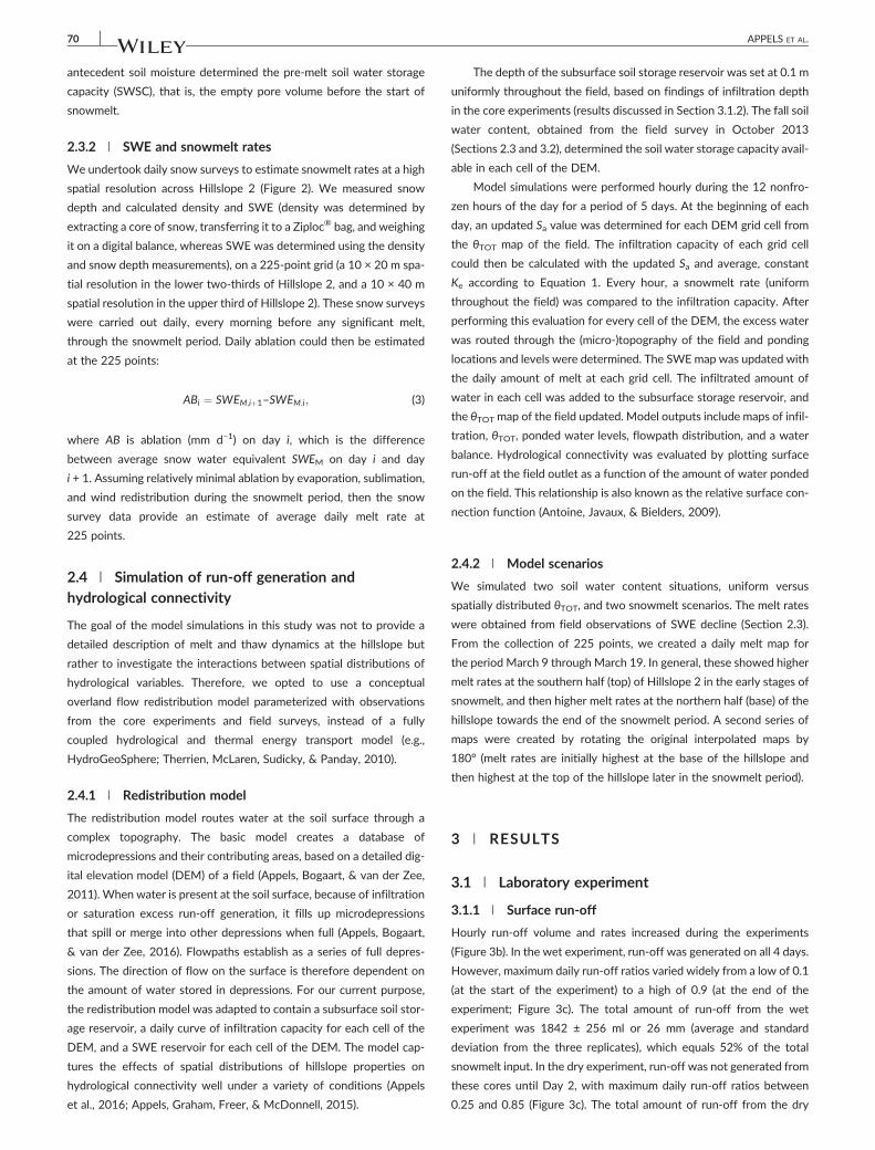
3.1.1 | Surface run‐off

Hourly run‐off volume and rates increased during the experiments

(Figure 3b). In the wet experiment, run‐off was generated on all 4 days.

However, maximum daily run‐off ratios varied widely from a low of 0.1

(at the start of the experiment) to a high of 0.9 (at the end of the

experiment; Figure 3c). The total amount of run‐off from the wet

experiment was 1842 ± 256 ml or 26 mm (average and standard

deviation from the three replicates), which equals 52% of the total

snowmelt input. In the dry experiment, run‐off was not generated from

these cores until Day 2, with maximum daily run‐off ratios between

0.25 and 0.85 (Figure 3c). The total amount of run‐off from the dry

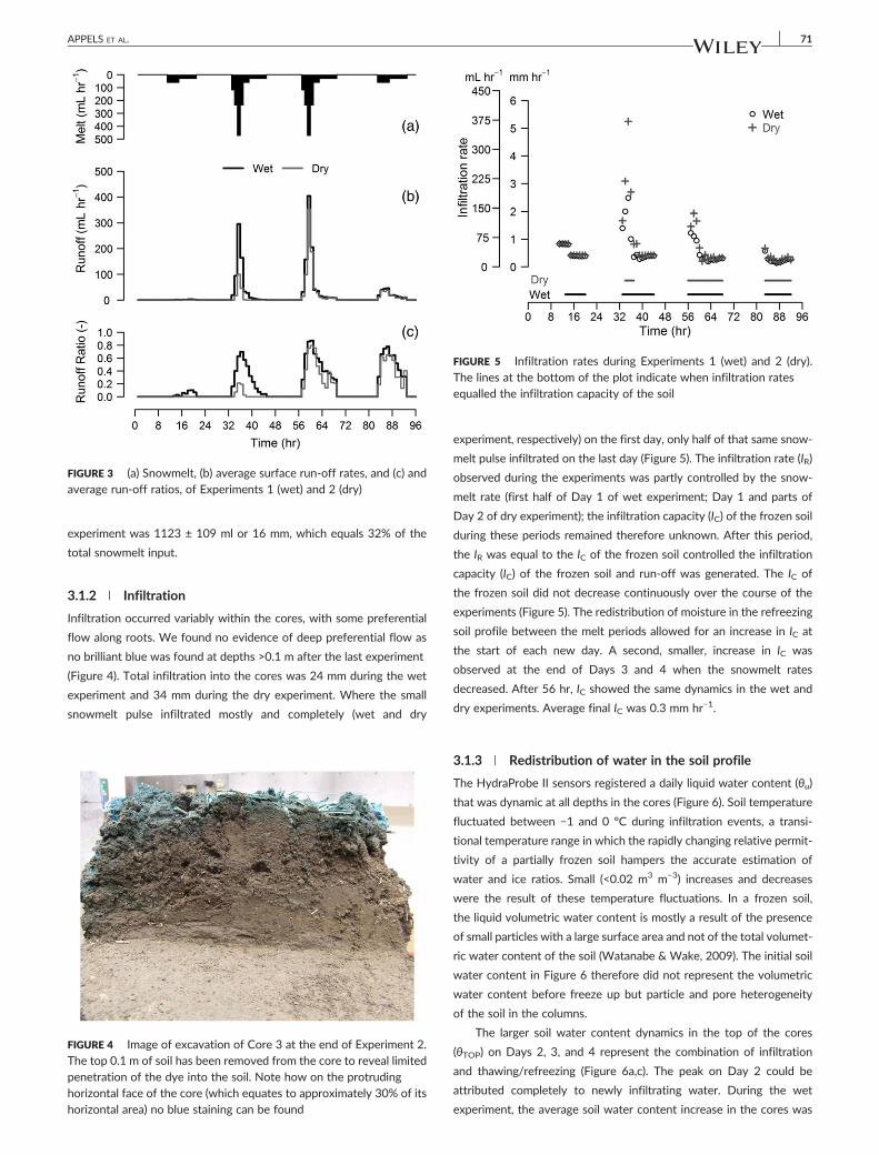
FIGURE 3 (a) Snowmelt, (b) average surface run‐off rates, and (c) andaverage run‐off ratios, of Experiments 1 (wet) and 2 (dry)

FIGURE 5 Infiltration rates during Experiments 1 (wet) and 2 (dry).The lines at the bottom of the plot indicate when infiltration ratesequalled the infiltration capacity of the soil

APPELS ET AL. 71

experiment was 1123 ± 109 ml or 16 mm, which equals 32% of the

total snowmelt input.

3.1.2 | Infiltration

Infiltration occurred variably within the cores, with some preferential

flow along roots. We found no evidence of deep preferential flow as

no brilliant blue was found at depths >0.1 m after the last experiment

(Figure 4). Total infiltration into the cores was 24 mm during the wet

experiment and 34 mm during the dry experiment. Where the small

snowmelt pulse infiltrated mostly and completely (wet and dry

FIGURE 4 Image of excavation of Core 3 at the end of Experiment 2.The top 0.1 m of soil has been removed from the core to reveal limitedpenetration of the dye into the soil. Note how on the protrudinghorizontal face of the core (which equates to approximately 30% of itshorizontal area) no blue staining can be found

experiment, respectively) on the first day, only half of that same snow-

melt pulse infiltrated on the last day (Figure 5). The infiltration rate (IR)

observed during the experiments was partly controlled by the snow-

melt rate (first half of Day 1 of wet experiment; Day 1 and parts of

Day 2 of dry experiment); the infiltration capacity (IC) of the frozen soil

during these periods remained therefore unknown. After this period,

the IR was equal to the IC of the frozen soil controlled the infiltration

capacity (IC) of the frozen soil and run‐off was generated. The IC of

the frozen soil did not decrease continuously over the course of the

experiments (Figure 5). The redistribution of moisture in the refreezing

soil profile between the melt periods allowed for an increase in IC at

the start of each new day. A second, smaller, increase in IC was

observed at the end of Days 3 and 4 when the snowmelt rates

decreased. After 56 hr, IC showed the same dynamics in the wet and

dry experiments. Average final IC was 0.3 mm hr−1.

3.1.3 | Redistribution of water in the soil profile

The HydraProbe II sensors registered a daily liquid water content (θu)

that was dynamic at all depths in the cores (Figure 6). Soil temperature

fluctuated between −1 and 0 °C during infiltration events, a transi-

tional temperature range in which the rapidly changing relative permit-

tivity of a partially frozen soil hampers the accurate estimation of

water and ice ratios. Small (<0.02 m3 m−3) increases and decreases

were the result of these temperature fluctuations. In a frozen soil,

the liquid volumetric water content is mostly a result of the presence

of small particles with a large surface area and not of the total volumet-

ric water content of the soil (Watanabe & Wake, 2009). The initial soil

water content in Figure 6 therefore did not represent the volumetric

water content before freeze up but particle and pore heterogeneity

of the soil in the columns.

The larger soil water content dynamics in the top of the cores

(θTOP) on Days 2, 3, and 4 represent the combination of infiltration

and thawing/refreezing (Figure 6a,c). The peak on Day 2 could be

attributed completely to newly infiltrating water. During the wet

experiment, the average soil water content increase in the cores was

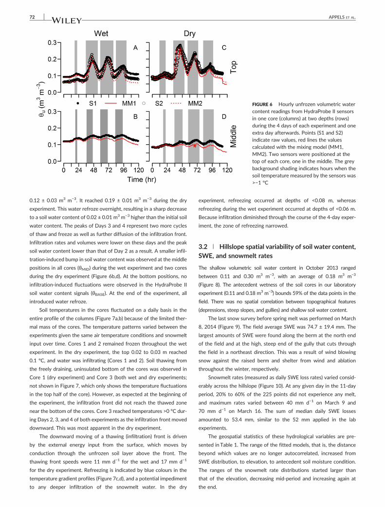
FIGURE 6 Hourly unfrozen volumetric watercontent readings from HydraProbe II sensorsin one core (columns) at two depths (rows)during the 4 days of each experiment and oneextra day afterwards. Points (S1 and S2)indicate raw values, red lines the valuescalculated with the mixing model (MM1,MM2). Two sensors were positioned at thetop of each core, one in the middle. The greybackground shading indicates hours when thesoil temperature measured by the sensors was>−1 °C

72 APPELS ET AL.

0.12 ± 0.03 m3 m−3. It reached 0.19 ± 0.01 m3 m−3 during the dry

experiment. This water refroze overnight, resulting in a sharp decrease

to a soil water content of 0.02 ± 0.01 m3 m−3 higher than the initial soil

water content. The peaks of Days 3 and 4 represent two more cycles

of thaw and freeze as well as further diffusion of the infiltration front.

Infiltration rates and volumes were lower on these days and the peak

soil water content lower than that of Day 2 as a result. A smaller infil-

tration‐induced bump in soil water content was observed at the middle

positions in all cores (θMID) during the wet experiment and two cores

during the dry experiment (Figure 6b,d). At the bottom positions, no

infiltration‐induced fluctuations were observed in the HydraProbe II

soil water content signals (θBASE). At the end of the experiment, all

introduced water refroze.

Soil temperatures in the cores fluctuated on a daily basis in the

entire profile of the columns (Figure 7a,b) because of the limited ther-

mal mass of the cores. The temperature patterns varied between the

experiments given the same air temperature conditions and snowmelt

input over time. Cores 1 and 2 remained frozen throughout the wet

experiment. In the dry experiment, the top 0.02 to 0.03 m reached

0.1 °C, and water was infiltrating (Cores 1 and 2). Soil thawing from

the freely draining, uninsulated bottom of the cores was observed in

Core 1 (dry experiment) and Core 3 (both wet and dry experiments;

not shown in Figure 7, which only shows the temperature fluctuations

in the top half of the core). However, as expected at the beginning of

the experiment, the infiltration front did not reach the thawed zone

near the bottom of the cores. Core 3 reached temperatures >0 °C dur-

ing Days 2, 3, and 4 of both experiments as the infiltration front moved

downward. This was most apparent in the dry experiment.

The downward moving of a thawing (infiltration) front is driven

by the external energy input from the surface, which moves by

conduction through the unfrozen soil layer above the front. The

thawing front speeds were 11 mm d−1 for the wet and 17 mm d−1

for the dry experiment. Refreezing is indicated by blue colours in the

temperature gradient profiles (Figure 7c,d), and a potential impediment

to any deeper infiltration of the snowmelt water. In the dry

experiment, refreezing occurred at depths of <0.08 m, whereas

refreezing during the wet experiment occurred at depths of <0.06 m.

Because infiltration diminished through the course of the 4‐day exper-

iment, the zone of refreezing narrowed.

3.2 | Hillslope spatial variability of soil water content,SWE, and snowmelt rates

The shallow volumetric soil water content in October 2013 ranged

between 0.11 and 0.30 m3 m−3, with an average of 0.18 m3 m−3

(Figure 8). The antecedent wetness of the soil cores in our laboratory

experiment (0.11 and 0.18 m3 m−3) bounds 59% of the data points in the

field. There was no spatial correlation between topographical features

(depressions, steep slopes, and gullies) and shallow soil water content.

The last snow survey before spring melt was performed on March

8, 2014 (Figure 9). The field average SWE was 74.7 ± 19.4 mm. The

largest amounts of SWE were found along the berm at the north end

of the field and at the high, steep end of the gully that cuts through

the field in a northeast direction. This was a result of wind blowing

snow against the raised berm and shelter from wind and ablation

throughout the winter, respectively.

Snowmelt rates (measured as daily SWE loss rates) varied consid-

erably across the hillslope (Figure 10). At any given day in the 11‐day

period, 20% to 60% of the 225 points did not experience any melt,

and maximum rates varied between 40 mm d−1 on March 9 and

70 mm d−1 on March 16. The sum of median daily SWE losses

amounted to 53.4 mm, similar to the 52 mm applied in the lab

experiments.

The geospatial statistics of these hydrological variables are pre-

sented in Table 1. The range of the fitted models, that is, the distance

beyond which values are no longer autocorrelated, increased from

SWE distribution, to elevation, to antecedent soil moisture condition.

The ranges of the snowmelt rate distributions started larger than

that of the elevation, decreasing mid‐period and increasing again at

the end.

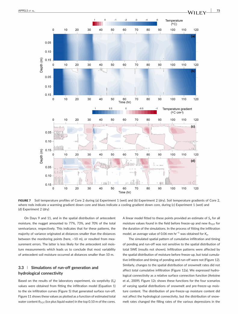
FIGURE 7 Soil temperature profiles of Core 2 during (a) Experiment 1 (wet) and (b) Experiment 2 (dry). Soil temperature gradients of Core 2,

where reds indicate a warming gradient down core and blues indicate a cooling gradient down core, during (c) Experiment 1 (wet) and(d) Experiment 2 (dry)

APPELS ET AL. 73

On Days 9 and 11, and in the spatial distribution of antecedent

moisture, the nugget amounted to 77%, 73%, and 70% of the total

semivariance, respectively. This indicates that for these patterns, the

majority of variance originated at distances smaller than the distances

between the monitoring points (here, ~10 m), or resulted from mea-

surement errors. The latter is less likely for the antecedent soil mois-

ture measurements which leads us to conclude that most variability

of antecedent soil moisture occurred at distances smaller than 10 m.

3.3 | Simulations of run‐off generation andhydrological connectivity

Based on the results of the laboratory experiment, six sorptivity (Sa)

values were obtained from fitting the infiltration model (Equation 1)

to the six infiltration curves (Figure 5) that generated surface run‐off.

Figure 11 shows these values as plotted as a function of estimated total

water content θTOT (ice plus liquid water) in the top 0.10 m of the cores.

A linear model fitted to these points provided an estimate of Sa for all

moisture values found in the field before freeze‐up and new θTOT for

the duration of the simulations. In the process of fitting the infiltration

model, an average value of 0.06 mm hr−1 was obtained for Ke.

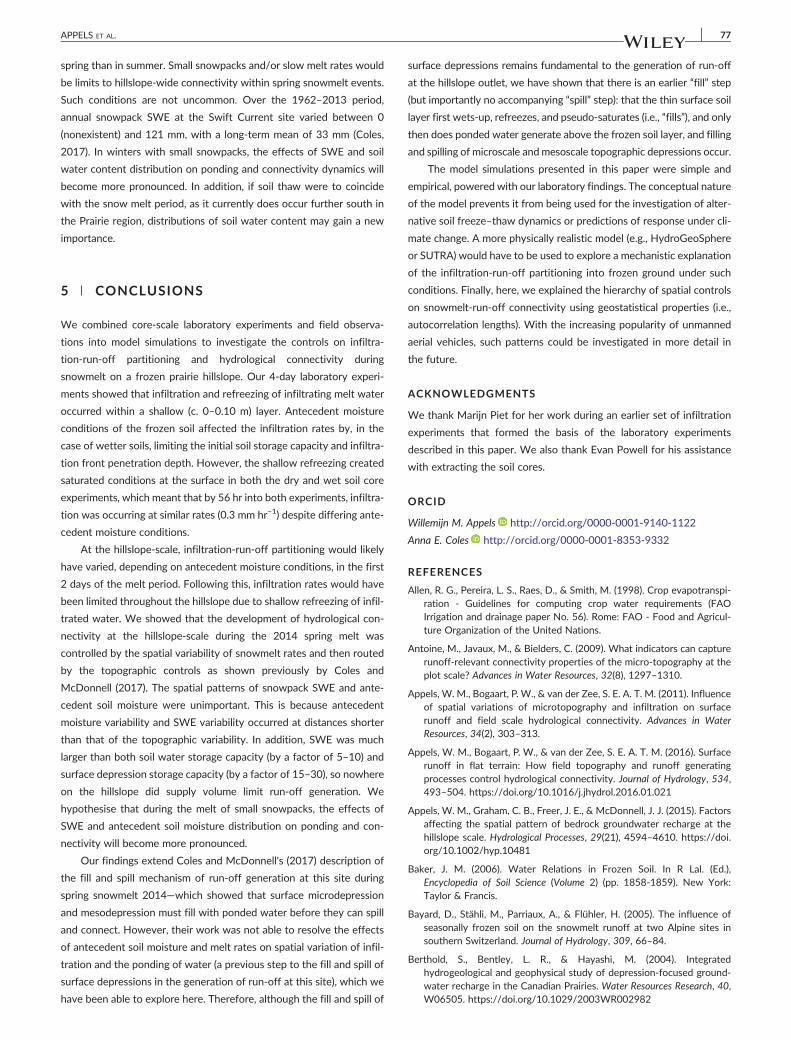
The simulated spatial pattern of cumulative infiltration and timing

of ponding and run‐off was not sensitive to the spatial distribution of

total SWE (results not shown). Infiltration patterns were affected by

the spatial distribution of moisture before freeze‐up, but total cumula-

tive infiltration and timing of ponding and run‐off were not (Figure 12).

Similarly, changes to the spatial distribution of snowmelt rates did not

affect total cumulative infiltration (Figure 12a). We expressed hydro-

logical connectivity as a relative surface connection function (Antoine

et al., 2009). Figure 12c shows these functions for the four scenarios

of varying spatial distributions of snowmelt and pre‐freeze‐up mois-

ture content. The distribution of pre‐freeze‐up moisture content did

not affect the hydrological connectivity, but the distribution of snow-

melt rates changed the filling rates of the various depressions in the

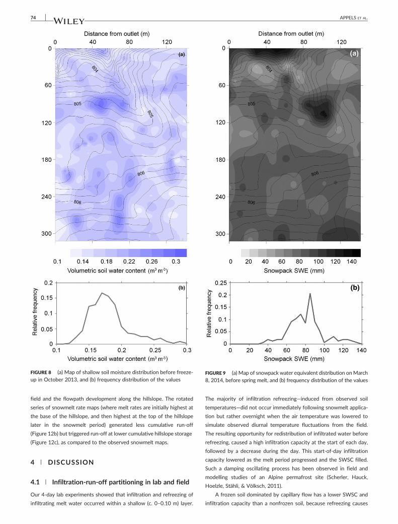
FIGURE 8 (a) Map of shallow soil moisture distribution before freeze‐up in October 2013, and (b) frequency distribution of the values

FIGURE 9 (a) Map of snowpack water equivalent distribution onMarch8, 2014, before spring melt, and (b) frequency distribution of the values

74 APPELS ET AL.

field and the flowpath development along the hillslope. The rotated

series of snowmelt rate maps (where melt rates are initially highest at

the base of the hillslope, and then highest at the top of the hillslope

later in the snowmelt period) generated less cumulative run‐off

(Figure 12b) but triggered run‐off at lower cumulative hillslope storage

(Figure 12c), as compared to the observed snowmelt maps.

4 | DISCUSSION

4.1 | Infiltration‐run‐off partitioning in lab and field

Our 4‐day lab experiments showed that infiltration and refreezing of

infiltrating melt water occurred within a shallow (c. 0–0.10 m) layer.

The majority of infiltration refreezing—induced from observed soil

temperatures—did not occur immediately following snowmelt applica-

tion but rather overnight when the air temperature was lowered to

simulate observed diurnal temperature fluctuations from the field.

The resulting opportunity for redistribution of infiltrated water before

refreezing, caused a high infiltration capacity at the start of each day,

followed by a decrease during the day. This start‐of‐day infiltration

capacity lowered as the melt period progressed and the SWSC filled.

Such a damping oscillating process has been observed in field and

modelling studies of an Alpine permafrost site (Scherler, Hauck,

Hoelzle, Stähli, & Völksch, 2011).

A frozen soil dominated by capillary flow has a lower SWSC and

infiltration capacity than a nonfrozen soil, because refreezing causes

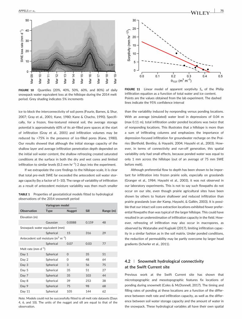
FIGURE 10 Quantiles (20%, 40%, 50%, 60%, and 80%) of dailysnowpack water equivalent loss at the hillslope during the 2014 meltperiod. Grey shading indicates 5% increments

FIGURE 11 Linear model of apparent sorptivity Sa of the Philipinfiltration equation as a function of total water and ice content.Points are the values obtained from the lab experiment. The dashedlines indicate the 95% confidence interval

APPELS ET AL. 75

ice to block the interconnectivity of soil pores (Fourie, Barnes, & Shur,

2007; Gray et al., 2001; Kane, 1980; Kane & Chacho, 1990). Specifi-

cally, for a frozen, fine‐textured mineral soil, the average storage

potential is approximately 60% of its air‐filled pore spaces at the start

of infiltration (Gray et al., 2001) and infiltration volumes may be

reduced by >75% in the presence of ice‐filled pores (Kane, 1980).

Our results showed that although the initial storage capacity of the

shallow layer and average infiltration penetration depth depended on

the initial soil water content, the shallow refreezing created saturated

conditions at the surface in both the dry and wet cores and limited

infiltration to similar levels (0.3 mm hr−1) 2 days into the experiment.

If we extrapolate the core findings to the hillslope‐scale, it is clear

that total pre‐melt SWE far exceeded the antecedent soil water stor-

age capacity (by a factor of 5–10). The range of variability of infiltration

as a result of antecedent moisture variability was then much smaller

TABLE 1 Properties of geostatistical models fitted to hydrological

observations of the 2014 snowmelt period

Observation

Variogram model

Sill Range (m)Type Nugget

Elevation (m)

Gaussian 0.0088 0.159 48

Snowpack water equivalent (mm)

Spherical 15 316 29

Antecedent soil moisture (m3 m−3)

Spherical 0.07 0.03 77

Melt rate (mm d−1)

Day 1 Spherical 0 35 51

Day 2 Spherical 0 48 64

Day 3 Spherical 3 56 75

Day 5 Spherical 35 51 27

Day 7 Spherical 35 103 44

Day 8 Spherical 39 253 38

Day 9 Spherical 75 98 68

Day 11 Spherical 105 144 62

Note. Models could not be successfully fitted to all melt rate datasets (Days4, 6, and 10). The units of the nugget and sill are equal to that of theobservation.

than the variability induced by nonponding versus ponding locations.

With an average (simulated) water level in depressions of 0.04 m

(max 0.11 m), total infiltration under ponded locations was twice that

of nonponding locations. This illustrates that a hillslope is more than

a sum of infiltrating columns and emphasizes the importance of

depression‐focused infiltration for groundwater recharge on the Prai-

ries (Berthold, Bentley, & Hayashi, 2004; Hayashi et al., 2003). How-

ever, in terms of connectivity and run‐off generation, this spatial

variability only had small effects, because ponded water was equal to

only 1 mm across the hillslope (out of an average of 75 mm SWE

before melt).

Although preferential flow to depth has been shown to be impor-

tant for infiltration into frozen prairie soils, especially on grasslands

(Granger et al., 1984; Hayashi et al., 2003), it was not observed in

our laboratory experiments. This is not to say such flowpaths do not

occur on our site, even though prairie agricultural sites have been

shown by others to feature shallower and reduced infiltration than

prairie grasslands (van der Kamp, Hayashi, & Gallén, 2003). It is possi-

ble that our intact soil core extraction locations exhibited fewer prefer-

ential flowpaths than was typical of the larger hillslope. This could have

resulted in an underestimation of infiltration capacity in the field. How-

ever, refreezing of infiltration may also occur in macropores, as

observed by Watanabe and Kugisaki (2017), limiting infiltration capac-

ity in a similar fashion as in the soil matrix. Under ponded conditions,

the reduction of permeability may be partly overcome by larger head

gradients (Scherler et al., 2011).

4.2 | Snowmelt hydrological connectivityat the Swift Current site

Previous work at the Swift Current site has shown that

microtopographic and mesotopographic features fix locations of

ponding during snowmelt (Coles & McDonnell, 2017). The timing and

filling rates of ponding at these locations are a function of the differ-

ence between melt rate and infiltration capacity, as well as the differ-

ence between soil water storage capacity and the amount of water in

the snowpack. These hydrological variables all have their own spatial

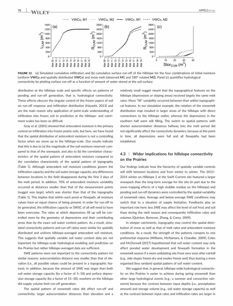
FIGURE 12 (a) Simulated cumulative infiltration and (b) cumulative surface run‐off of the hillslope for the four combinations of initial moisture(uniform VWCu and spatially distributed VWCv) and snow melt (observed M1 and 180° rotated M2). Panel (c) quantifies hydrologicalconnectivity by plotting surface run‐off as a function of amount of water stored at the soil surface

76 APPELS ET AL.

distribution at the hillslope scale and specific effects on patterns of

ponding and run‐off generation, that is, hydrological connectivity.

These effects obscure the singular control of the frozen aspect of soil

on run‐off response and infiltration distribution (Hayashi, 2013) and

are the main reason why application of point‐scale understanding of

infiltration into frozen soil to prediction at the hillslope‐ and catch-

ment‐scales has been so difficult.

Gray et al. (2001) showed that antecedent moisture is the primary

control on infiltration into frozen prairie soils, but here, we have found

that the spatial distribution of antecedent moisture is not a controlling

factor when we move up to the hillslope‐scale. Our results indicate

that this is due to (a) the magnitude of the soil moisture reservoir com-

pared to that of the snowpack, and also to (b) the correlation charac-

teristics of the spatial pattern of antecedent moisture compared to

the correlation characteristic of the spatial pattern of topography

(Table 1). Although antecedent soil moisture conditions govern the

infiltration capacity and the soil water storage capacity, any differences

between locations in the field disappeared during the first 3 days of

the melt period. In addition, 70% of antecedent moisture variability

occurred at distances smaller than that of the measurement points

(nugget was large), which was shorter than that of the topography

(Table 1). This implies that within each pond or flowpath, all moisture

values have an equal chance of being present; in order for run‐off to

be generated, the infiltration capacity or SWSC of all will need to have

been overcome. The rates at which depressions fill up will be con-

trolled more by the geometry of depressions and their contributing

areas than by the exact soil water content pattern. As a result, simu-

lated connectivity patterns and run‐off ratios were similar for spatially

distributed and uniform hillslope‐averaged antecedent soil moisture.

This suggests that spatially variable soil water content data are not

important for hillslope‐scale hydrological modeling and prediction on

the Prairies but rather hillslope‐averaged data are sufficient.

SWE patterns were not important to the connectivity pattern for

similar reasons: autocorrelation distance was smaller than that of ele-

vation (i.e., all possible values could be present in a topographic fea-

ture). In addition, because the amount of SWE was larger than both

soil water storage capacity (by a factor of 5–10) and surface depres-

sion storage capacity (by a factor of 15–30), nowhere on the hillslope

did supply volume limit run‐off generation.

The spatial pattern of snowmelt rates did affect run‐off and

connectivity: larger autocorrelation distances than elevation and a

relatively small nugget meant that the topographical features on the

hillslope (depressions or sloping areas) received largely the same melt

rates. More “fill” variability occurred between than within topographi-

cal features. In our simulation example, the rotation of the snowmelt

distribution map resulted in larger areas of the hillslope with direct

connections to the hillslope outlet, whereas the depressions in the

southern half were still filling. The switch to spatial patterns with

shorter autocorrelation distances halfway into the melt period did

not significantly affect the connectivity dynamics, because at this point

in time, all depressions were full and all flowpaths had been

established.

4.3 | Wider implications for hillslope connectivityon the Prairies

Our findings indicate how the hierarchy of spatially variable controls

will shift between locations and from winter to winter. The 2013–

2014 winter on Hillslope 2 at the Swift Current site featured a larger

snowpack than the long‐term average for the site (in part due to the

snow trapping effects of a high stubble residue on the hillslope) and

ponding and run‐off dynamics were controlled by the spatial variability

of snowmelt rates. Average and below‐average SWE conditions may

switch that to a situation of supply limitation. Feedbacks play an

important role here: less SWE may affect the level of soil frost and soil

thaw during the melt season and consequently infiltration rates and

volumes (Quinton, Bemrose, Zhang, & Carey, 2009).

In steeper catchments, topography may control the spatial distri-

bution of snow as well as that of melt rates and antecedent moisture

conditions. As a result, the strength of the patterns conspire to one

preferential response (Williams, McNamara, & Chandler, 2009). Coles

and McDonnell (2017) hypothesized that soil water content may only

affect ponded water development and flowpath formation in the

snowmelt season if a more undulating site froze very soon after rainfall

(e.g., side slopes freeze dry and swales freeze wet) thus leaving a more

organised (less random) spatial pattern of soil water content.

We suggest that, in general, hillslope‐wide hydrological connectiv-

ity on the Prairies is easier to achieve during spring snowmelt than

other large hydrological events (e.g., a summer and convective rain-

storm) because the contrast between input depths (i.e., precipitation

amount) and storage volume (e.g., soil water storage capacity) as well

as the contrast between input rates and infiltration rates are larger in

APPELS ET AL. 77

spring than in summer. Small snowpacks and/or slow melt rates would

be limits to hillslope‐wide connectivity within spring snowmelt events.

Such conditions are not uncommon. Over the 1962–2013 period,

annual snowpack SWE at the Swift Current site varied between 0

(nonexistent) and 121 mm, with a long‐term mean of 33 mm (Coles,

2017). In winters with small snowpacks, the effects of SWE and soil

water content distribution on ponding and connectivity dynamics will

become more pronounced. In addition, if soil thaw were to coincide

with the snow melt period, as it currently does occur further south in

the Prairie region, distributions of soil water content may gain a new

importance.

5 | CONCLUSIONS

We combined core‐scale laboratory experiments and field observa-

tions into model simulations to investigate the controls on infiltra-

tion‐run‐off partitioning and hydrological connectivity during

snowmelt on a frozen prairie hillslope. Our 4‐day laboratory experi-

ments showed that infiltration and refreezing of infiltrating melt water

occurred within a shallow (c. 0–0.10 m) layer. Antecedent moisture

conditions of the frozen soil affected the infiltration rates by, in the

case of wetter soils, limiting the initial soil storage capacity and infiltra-

tion front penetration depth. However, the shallow refreezing created

saturated conditions at the surface in both the dry and wet soil core

experiments, which meant that by 56 hr into both experiments, infiltra-

tion was occurring at similar rates (0.3 mm hr−1) despite differing ante-

cedent moisture conditions.

At the hillslope‐scale, infiltration‐run‐off partitioning would likely

have varied, depending on antecedent moisture conditions, in the first

2 days of the melt period. Following this, infiltration rates would have

been limited throughout the hillslope due to shallow refreezing of infil-

trated water. We showed that the development of hydrological con-

nectivity at the hillslope‐scale during the 2014 spring melt was

controlled by the spatial variability of snowmelt rates and then routed

by the topographic controls as shown previously by Coles and

McDonnell (2017). The spatial patterns of snowpack SWE and ante-

cedent soil moisture were unimportant. This is because antecedent

moisture variability and SWE variability occurred at distances shorter

than that of the topographic variability. In addition, SWE was much

larger than both soil water storage capacity (by a factor of 5–10) and

surface depression storage capacity (by a factor of 15–30), so nowhere

on the hillslope did supply volume limit run‐off generation. We

hypothesise that during the melt of small snowpacks, the effects of

SWE and antecedent soil moisture distribution on ponding and con-

nectivity will become more pronounced.

Our findings extend Coles and McDonnell's (2017) description of

the fill and spill mechanism of run‐off generation at this site during

spring snowmelt 2014—which showed that surface microdepression

and mesodepression must fill with ponded water before they can spill

and connect. However, their work was not able to resolve the effects

of antecedent soil moisture and melt rates on spatial variation of infil-

tration and the ponding of water (a previous step to the fill and spill of

surface depressions in the generation of run‐off at this site), which we

have been able to explore here. Therefore, although the fill and spill of

surface depressions remains fundamental to the generation of run‐off

at the hillslope outlet, we have shown that there is an earlier “fill” step

(but importantly no accompanying “spill” step): that the thin surface soil

layer first wets‐up, refreezes, and pseudo‐saturates (i.e., “fills”), and only

then does ponded water generate above the frozen soil layer, and filling

and spilling of microscale andmesoscale topographic depressions occur.

The model simulations presented in this paper were simple and

empirical, powered with our laboratory findings. The conceptual nature

of the model prevents it from being used for the investigation of alter-

native soil freeze–thaw dynamics or predictions of response under cli-

mate change. A more physically realistic model (e.g., HydroGeoSphere

or SUTRA) would have to be used to explore a mechanistic explanation

of the infiltration‐run‐off partitioning into frozen ground under such

conditions. Finally, here, we explained the hierarchy of spatial controls

on snowmelt‐run‐off connectivity using geostatistical properties (i.e.,

autocorrelation lengths). With the increasing popularity of unmanned

aerial vehicles, such patterns could be investigated in more detail in

the future.

ACKNOWLEDGMENTS

We thank Marijn Piet for her work during an earlier set of infiltration

experiments that formed the basis of the laboratory experiments

described in this paper. We also thank Evan Powell for his assistance

with extracting the soil cores.

ORCID

Willemijn M. Appels http://orcid.org/0000-0001-9140-1122

Anna E. Coles http://orcid.org/0000-0001-8353-9332

REFERENCES

Allen, R. G., Pereira, L. S., Raes, D., & Smith, M. (1998). Crop evapotranspi-ration ‐ Guidelines for computing crop water requirements (FAOIrrigation and drainage paper No. 56). Rome: FAO ‐ Food and Agricul-ture Organization of the United Nations.

Antoine, M., Javaux, M., & Bielders, C. (2009). What indicators can capturerunoff‐relevant connectivity properties of the micro‐topography at theplot scale? Advances in Water Resources, 32(8), 1297–1310.

Appels, W. M., Bogaart, P. W., & van der Zee, S. E. A. T. M. (2011). Influenceof spatial variations of microtopography and infiltration on surfacerunoff and field scale hydrological connectivity. Advances in WaterResources, 34(2), 303–313.

Appels, W. M., Bogaart, P. W., & van der Zee, S. E. A. T. M. (2016). Surfacerunoff in flat terrain: How field topography and runoff generatingprocesses control hydrological connectivity. Journal of Hydrology, 534,493–504. https://doi.org/10.1016/j.jhydrol.2016.01.021

Appels, W. M., Graham, C. B., Freer, J. E., & McDonnell, J. J. (2015). Factorsaffecting the spatial pattern of bedrock groundwater recharge at thehillslope scale. Hydrological Processes, 29(21), 4594–4610. https://doi.org/10.1002/hyp.10481

Baker, J. M. (2006). Water Relations in Frozen Soil. In R Lal. (Ed.),Encyclopedia of Soil Science (Volume 2) (pp. 1858‐1859). New York:Taylor & Francis.

Bayard, D., Stähli, M., Parriaux, A., & Flühler, H. (2005). The influence ofseasonally frozen soil on the snowmelt runoff at two Alpine sites insouthern Switzerland. Journal of Hydrology, 309, 66–84.

Berthold, S., Bentley, L. R., & Hayashi, M. (2004). Integratedhydrogeological and geophysical study of depression‐focused ground-water recharge in the Canadian Prairies. Water Resources Research, 40,W06505. https://doi.org/10.1029/2003WR002982

78 APPELS ET AL.

Birchak, J. R., Gardner, C. G., Hipp, J. E., & Victor, J. M. (1974). High dielec-tric constant microwave probes for sensing soil moisture. Proceedings ofthe IEEE, 62(1), 93–98.

Coles, A. E. (2017). Runoff generation over seasonally‐frozen ground:Trends, patterns, and processes. Ph.D. Thesis. Saskatoon: Universityof Saskatchewan.

Coles, A. E., McConkey, B. G., & McDonnell, J. J. (2017). Climate changeimpacts on hillslope runoff on the northern Great Plains, 1962‐2013.Journal of Hydrology. https://doi.org/10.1016/j.jhydrol.2017.05.023

Coles, A. E. & McDonnell, J. J. (2017). Fill and spill drives runoff connectiv-ity over frozen ground, Manuscript under review with Journal ofHydrology.

Fang, X., & Pomeroy, J. W. (2007). Snowmelt runoff sensitivity analysisto drought on the Canadian prairies. Hydrological Processes, 21,2594–2609. https://doi.org/10.1002/hyp.6796

Flury, M., Flühler, H., Jury, W. A., & Leuenberger, J. (1994). Susceptibility ofsoils to preferential flow of water: A field study. Water ResourcesResearch, 30(7), 1945–1954.

Fourie, W. J., Barnes, D. L., & Shur, Y. (2007). The formation of ice from theinfiltration of water into a frozen coarse grained soil. Cold RegionsScience and Technology, 48(2), 118–128. https://doi.org/10.1016/j.coldregions.2006.09.004

Gräler, B., Pebesma, E., & Heuvelink, G. (2016). Spatio‐temporal Interpola-tion using gstat. The R Journal, 8(1), 204–218.

Granger, R., Gray, D., & Dyck, G. E. (1984). Snowmelt infiltration to frozenprairie soils. Canadian Journal of Earth Sciences, 21(6), 669–677.

Gray, D. M., Landine, P. G., & Granger, R. J. (1985). Simulating infiltrationinto frozen Prairie soils in streamflow models. Canadian Journal of EarthSciences, 22(3), 464–472.

Gray, D. M., Norum, D. I., & Granger, R. J. (1984). The prairie soil moistureregime: fall to seeding. Presented at: Optimum Tillage ChallengeWorkshop, p17899.

Gray, D. M., Toth, B., Zhao, L., Pomeroy, J. W., & Granger, R. J. (2001).Estimating areal snowmelt infiltration into frozen soils. Hydrological Pro-cesses, 15, 3095–3111.

Gupta, H. V. & Sorooshian, S. (1997). The challenges we face: panel discus-sion on snow. In S. Sorooshian, H. V. Gupta, & J. C. Rodda (Eds.) LandSurface Processes in Hydrology: Trials and Tribulations of Modeling andMeasuring. NATO ASI Series (Vol. I 46) (pp. 183‐187). Verlag BerlinHeidelberg New York: Springer.

Hansson, K., Šimůnek, J., Mizoguchi, M., Lundin, L., & van Genuchten, M. T.(2004). Water flow and heat transport in frozen soil: numerical solutionand freeze‐thaw applications. Vadose Zone Journal, 3, 693–704. https://doi.org/10.2136/vzj2004.0693.

Hayashi, M. (2013). The Cold Vadose Zone: Hydrological and EcologicalSignificance of Frozen‐Soil Processes. Vadose Zone Journal, 12(4).https://doi.org/10.2136/vzj2013.03.0064.

Hayashi, M., van der Kamp, G., & Schmidt, R. (2003). Focused infiltration ofsnowmelt water in partially frozen soil under small depressions. Journalof Hydrology, 270(3–4), 214–229. https://doi.org/10.1016/S0022‐1694(02)00287‐1

Ireson, A. M., van der Kamp, G., Ferguson, G. A. G., Nachson, U., &Wheater, H. S. (2013). Hydrogeological processes in seasonally frozennorthern latitudes: Understanding, gaps and challenges. HydrogeologyJournal, 21, 53–66. https://doi.org/10.1007/s10040‐012‐0916‐5

Ishikawa, M., Zhang, Y., Kadota, T., & Ohata, T. (2006). Hydrothermalregimes of the dry active layer.Water Resources Research, 42, W04401.

Iwata, Y., Hayashi, M., Suzuki, S., Hirota, T., & Hasegawa, S. (2010). Effectsof snow cover on soil freezing, water movement, and snowmelt infiltra-tion: A paired plot experiment. Water Resources Research, 46, W09504.

Jansson, P.‐E., & Karlberg, L. (2001). Coupled heat and mass transfer modelfor soil‐plant‐atmosphere systems. Stockholm: Royal Institute of Tech-nology, Department of Civil and Environmental Engineering.

Kane, D. L. (1980). Snowmelt infiltration into seasonally frozen soils. ColdRegions Science and Technology, 3, 153–161. https://doi.org/10.1016/0165‐232X(80)90020‐8

Kane, D. L., & Chacho, E. F. (1990). Frozen ground effects on infiltrationand runoff. In W. L. Ryan, & R. D. Crissman (Eds.), Cold regions hydrologyand hydraulics (pp. 259–300). New York: American Society of CivilEngineers.

Kane, D. L., Hinkel, K. M., Goering, D. J., Hinzman, L. D., & Outcalt, S. I.(2001). Non‐conductive heat transfer associated with frozen soils.Global and Planetary Change, 29, 275–292.

Kane, D. L., & Stein, J. (1983). Water movement into seasonally frozen soils.Water Resources Research, 19(6), 1547–1557.

Kane, D. L., & Stein, J. (1984). Plot measurements of snowmelt runoff forvarying soil conditions. Geophysica, 20(2), 123–135.

Kitterød, N. O. (2008). Focused flow in the unsaturated zone after surfaceponding of snowmelt. Cold Regions Science and Technology, 53(1),42–55.

Li, L., & Simonovic, S. P. (2002). System dynamics model for predictingfloods from snowmelt in North American prairie watersheds. Hydrolog-ical Processes, 16, 2645–2666.

Lilbæk, G., & Pomeroy, J. W. (2010). Laboratory evidence for enhancedinfiltration of ion load during snowmelt. Hydrology and Earth SystemSciences, 14, 1365–1374.

Ling, F., & Zhang, T. (2004). A numerical model for surface energy balanceand thermal regime of the active layer and permafrost containing unfro-zen water. Cold Regions Science and Technology, 38(1), 1–15.

McCauley, C. A., White, D. M., Lilly, M. R., & Nyman, D. M. (2002). A com-parison of hydraulic conductivities, permeabilities and infiltration ratesin frozen and unfrozen soils. Cold Regions Science and Technology,34(2), 117–125. https://doi.org/10.1016/S0165‐232X(01)00064‐7

McConkey, B. G., Ulrich, D. J., & Dyck, F. B. (1997). Slope position andsubsoiling effects on soil water and spring wheat yield. Canadian Journalof Soil Science, 77, 83–90.

Moghadas, S., Gustafsson, A.‐M., Viklander, P., Marsalek, J., & Viklander, M.(2016). Laboratory study of infiltration into two frozen engineered(sandy) soils recommended for bioretention. Hydrological Processes,30, 1251–1264. https://doi.org/10.1002/hyp.10711

Motovilov, Y. G. (1978). Mathematical model of water infiltration intofrozen soils. Soviet Hydrology, 17(2), 62–66.

Motovilov, Y. G. (1979). Simulation of meltwater losses through infiltrationinto soil. Soviet Hydrology, 18(3), 217–221.

Painter, S. (2011). Three‐phase numerical model of water migration inpartially frozen geological media: Model formulation, validation, andapplications. Computational Geosciences, 15(1), 69–85.

Pebesma, E. J. (2004). Multivariable geostatistics in S: The gstat package.Computers & Geosciences, 30, 683–691.

Philip, J. R. (1957a). The theory of infiltration: 1. The infiltration equationand its solution. Soil Science, 83(5), 345–358.

Philip, J. R. (1957b). The theory of infiltration: 4. Sorptivity and algebraicinfiltration equations. Soil Science, 84(3), 257–264.

Pomeroy, J. W., Gray, D. M., Brown, T., Hedstrom, N. R., Quinton, W. L.,Granger, R. J., & Carey, S. K. (2007). The cold regions hydrologicalmodel: A platform for basing process representation and model struc-ture on physical evidence. Hydrological Processes, 21, 2650–2667.

Quinton, W. L., Bemrose, R. K., Zhang, Y., & Carey, S. K. (2009). The influ-ence of spatial variability in snowmelt and active layer thaw onhillslope drainage for an alpine tundra hillslope. Hydrological Processes,23, 2628–2639. https://doi.org/10.1002/hyp.7327

R CoreTeam (2016). R: A language and environment for statistical comput-ing. R Foundation for Statistical Computing, Vienna, Austria. URLhttps://www.r-project.org/

Romanovsky, V., & Osterkamp, T. (2000). Effects of unfrozen water on heatand mass transport processes in the active layer and permafrost. Perma-frost and Periglacial Processes, 11, 219–239.

APPELS ET AL. 79

Roth, K., Schulin, R., Flühler, H., & Attinger, W. (1990). Calibration of timedomain reflectometry for water content measurement using a compos-ite dielectric approach. Water Resources Research, 26, 2267–2273.

Scherler, M., Hauck, C., Hoelzle, M., Stähli, M., & Völksch, I. (2011). Meltwa-ter infiltration into the frozen active layer at an alpine permafrost site.Permafrost and Periglacial Processes, 2(4), 325–334.

Seyfried, M. S., & Murdock, M. D. (1996). Calibration of time domain reflec-tometry of measurement of liquid water in frozen soils. Soil Science,161, 87–98.

Spaans, E. J. A., & Baker, J. M. (1995). Examining the use of time domainreflectometry for measuring liquid water content in frozen soil. WaterResources Research, 31, 2917–2925. https://doi.org/10.1029/95WR02769

Stähli, M., Jansson, P.‐E., & Lundin, L.‐C. (1996). Preferential water flow in afrozen soil—A two‐domain model approach. Hydrological Processes, 10,1305–1316.

Stähli, M., Jansson, P.‐E., & Lundin, L.‐C. (1999). Soil moisture redistributionand infiltration in frozen sandy soils. Water Resources Research, 35(1),95–103. https://doi.org/10.1029/1998WR900045.

Su, J. J., van Bochove, E., Thériault, G., Novotna, B., Khaldoune, J., Denault,J. T., … Chow, T. L. (2011). Effects of snowmelt on phosphorus andsediment losses from agricultural watersheds in eastern Canada. Agri-cultural Water Management, 98(5), 867–876. https://doi.org/10.1016/j.agwat.2010.12.013

Therrien, R., McLaren, R. G., Sudicky, E. A., & Panday, S. M. (2010).HydroGeoSphere: A three‐dimensional numerical model describing fully‐integrated subsurface and surface flow and solute transport. Waterloo,ON: Groundwater Simulations Group, University of Waterloo.

Tindall, J. A., Hemmen, K., & Dowd, J. F. (1992). An improved method forfield extraction and laboratory analysis of large, intact soil cores. Journalof Environmental Quality, 21, 259–263.

van der Kamp, G., Hayashi, M., & Gallén, D. (2003). Comparing the hydrol-ogy of grassed and cultivated catchments in the semi‐arid Canadianprairies. Hydrological Processes, 17(3), 559–575.

Watanabe, K., Kito, T., Dun, S.,Wu, J. Q., Greer, R. C., & Flury,M. (2012).Waterinfiltration into a frozen soil with simultaneous melting of the frozen layer.Vadose Zone Journal, 12(1), 0. https://doi.org/10.2136/vzj2011.0188

Watanabe, K., & Kugisaki, Y. (2017). Effect of macropores on soil freezingand thawing with infiltration. Hydrological Processes, 31(2), 270.

Watanabe, K., & Wake, T. (2009). Measurement of unfrozen water contentand relative permittivity of frozen unsaturated soil using NMR andTDR. Cold Regions Science and Technology, 59(1), 34–41. https://doi.org/10.1016/j.coldregions.2009.05.011

Weiler, M., & Flühler, H. (2004). Inferring flow types from dye patterns inmacroporous soils. Geoderma, 120, 137–153.

Williams, C. J., McNamara, J. P., & Chandler, D. G. (2009). Controls on thetemporal and spatial variability of soil moisture in a mountainous land-scape: The signature of snow and complex terrain. Hydrology andEarth System Sciences, 13, 1325–1336.

Zhao, L., & Gray, D. M. (1997). A parametric expression for estimating infil-tration into frozen soils. Hydrological Processes, 11, 1761–1775.

Zhao, L., Gray, D. M., & Male, D. (1997). Numerical analysis of simultaneousheat and mass transfer during infiltration into frozen ground. Journal ofHydrology, 200, 345–363.

How to cite this article: Appels WM, Coles AE, McDonnell JJ.

Infiltration into frozen soil: From core‐scale dynamics to

hillslope‐scale connectivity. Hydrological Processes. 2018;32:

66–79. https://doi.org/10.1002/hyp.11399