72 • J. Nat. Resour. Life Sci. Educ., Vol. 34, 2005

ABSTRACT

One of the largest challenges in teaching introductory soil science is explaining the dynamics of soil infiltration. To aid stu-dents in understanding the concept and to further engage them in active learning in the soils laboratory course, we developed an exercise using Decagon Mini-Disk Infiltrometers with a tension head (ho) of 2 cm. Groups of up to four students measured cu-mulative infiltration for up to 5 minutes and plotted their results vs. time (t). Curves for each group were plotted using SigmaPlot through a computer-projection system so that students could observe infiltration differences between different soils. With the help of their lab instructors, regression analyses were completed to obtain curve-fitting parameters needed to calculate hydraulic conductivity (K). Upon completion of data analyses, the students worked cooperatively to answer several questions concerning infiltration physics. Based on student comments, we believe that we successfully engaged the students and increased their expo-sure and understanding of infiltration dynamics.

Because of the quantitative nature of teaching soil–water dynam-ics in introductory soil science courses, tools that allow students

to observe physical phenomenon usually aid the instructor in teach-ing these concepts. Thien (1973) placed enough importance on infil-tration and runoff that he developed it as 1 of 30 mini-courses used to supplement introductory soil science lectures. Helsel and Hughes (1984) found that 1 of 36 areas where urban students felt less com-petent than rural students was the ability to “explain the importance of soil physical properties on infiltration, percolation and runoff.” Their solution to building the urban student’s confidence was the production of 7- to 8-minute videotapes on each topic.

The specific physics and math required to quantify infiltration or hydraulic conductivity are beyond the capability of most introduc-tory soil science students. The use of Decagon Mini-Disk Infiltrom-eters (cost ~$50 each; Pullman, WA), however, allows students to observe and graph infiltration dynamics for different soil textures, statistically determine empirical parameters, and calculate hydraulic conductivity.

Decagon Devices (1998) recommends utilizing the approach of Zhang (1997) to determine hydraulic conductivity from the cumu-lative infiltration measured with one of their infiltrometers. Zhang (1997) used a truncated Philip-type expression (Philip, 1957) to quantify cumulative infiltration as follows:

I = C1t 0.5 + C

2t [1]

where I is the cumulative infiltration (cm), t is time (seconds), C1 and

C2 are adjustable parameters related to sorptivity (S) and hydraulic

conductivity (K), respectively, at the pressure head ho maintained by

the infiltrometer. Considering here only K(ho), Zhang (1997) showed

that the conductivity could be simply estimated as follows:

K(ho) = C

2/A [2]

where A is a soil texture dependent dimensionless coefficient deter-mined empirically. Values of A have been tabulated for a wide range of soil textures (Table 1) assuming the van Genuchten type moisture retention function (van Genuchten, 1980) with texture class param-eters according to Carsel and Parrish (1988). The values in Table 1 correct those provided by Decagon that used the tension head (e.g., 2 cm) instead of the pressure head (e.g., −2 cm) as required in Eq. [21] and [22] of Zhang (1997). A pressure head of −2 cm is close enough to saturation (h

o = 0 cm) that we would still have rapid flow

while preventing the need for a retaining ring to contain surface ponding at h

o = 0 cm.

An illustration of the anticipated infiltration characteristics is helpful in introducing the laboratory exercise. Figure 1 shows a two-dimensional representation of the soil wetting after 5 minutes of infiltration (Fig. 1A) and the corresponding experimental results the students can expect (Fig. 1B). Noting that at any time the slope of the I vs. t graph is the infiltration rate, students are instructed to expect higher rates in the coarser-textured soil. By the combination of matric and gravitational forces, the water movement is outward and downward from the infiltrometer with the greatest depth of wet-ting in the coarsest (highest K) soil (Fig. 1A). Students should be encouraged to verify this with a visual inspection of the wetted soil volume at the conclusion of the data collection.

MATERIALS AND METHODS

Properties of the four soils used in our exercise are listed in Ta-ble 2. We prepared air-dried soils by crushing them to pass a 2-mm sieve. We then added each soil to separate 5.3-L (30 cm long by 19 cm wide by 9.3 cm tall) Rubbermaid Plastic Clear tubs to approxi-mately 75% of the tubs’ capacity. The students then completed the exercise provided in Table 3.

We used a small, slotted scoop to remove the wetted Terry very fine sandy loam soil (coarse-loamy, mixed, superactive, mesic Ustic

An Infiltration Exercise for Introductory Soil Science

K. A. Barbarick,* J. A. Ippolito, G. Butters, and G. M. Sorge

Department of Soil and Crop Sciences, 200 W. Lake Street, Colorado State Univ., Fort Collins, CO 80523-1170. Received 25 Mar. 2005. *Correspond-ing author (ken.barbarick@colostate.edu).

Published in J. Nat. Resour. Life Sci. Educ. 34:72-76 (2005).http://www.JNRLSE.org© American Society of Agronomy677 S. Segoe Rd., Madison, WI 53711 USA

Table 1. Texture dependent dimensionless coefficient in Eq. [2] accord-ing to Zhang (1997).

Soil textureA parameter (Eq. [2])

(ho = −2 cm)

infiltrometer radius = 1.59 cm

Sand 2.37Loamy sand 3.33Sandy loam 5.36Loam 8.60Silt 11.95Silt loam 10.88Sandy clay loam 5.82Clay loam 9.11Silty clay loam 11.67Sandy clay 5.61Silty clay 8.72Clay 5.90

J. Nat. Resour. Life Sci. Educ., Vol. 34 2005 • 73

Table 2. Soil characteristics for infiltration exercise in Introductory Soil Science (SC240).

Mapping unitor soil name Soil taxonomy A

(Table 1) C

2 (from regression

analysis of Eq. [1]; see Fig. 6)

z, hydraulic conductivity(cm sec−1; estimated from

Eq. [2])

“Play” sand unclassified 2.37 0.17 5.5 × 10−2

Terry very fine sandy loam

coarse-loamy, mixed, superactive, mesic Ustic Haplargids 10.88 0.038 3.4 × 10−3

Bresser sandy loam fine-loamy, mixed, superactive, mesic Aridic Argiustolls 5.36 0.012 2.3 × 10−3

Nunn clay loam fine, smectitic, mesic Aridic Argi-ustolls 9.11 0.0030 3.3 × 10−4

Table 3. Infiltration exercise completed by Introductory Soil Science students working in groups of three or four.

Infiltration and hydraulic conductivity experimental procedure

Objective is to measure cumulative infiltration and estimate hydraulic conductivity using a Decagon Disk Infiltrometer.

1. Each group of students will measure cumulative infiltration in a soil using a 2.0-cm tension head Decagon Mini-Disk Infiltrometer at 15-second inter-vals for 5 minutes (300 seconds).

2. Fill the disk Infiltrometer by complete submergence in tap water and inserting the stopper while the infiltrometer is under water. Then set the infil-trometer to the 0 mL mark by placing the porous plate on a paper towel.

3. Select individuals to complete the following tasks: (i) observe the water level in the infiltrometers for each 15-second interval, (ii) record the water level for each time interval on Data Sheet 1, (iii) time each 15-second increment.

4. Secure the infiltrometers in the clamp attached to a ring stand (Fig. 2).

5. Lower the clamp plus infiltrometer to the surface of the soil (Fig. 3) and immediately begin timing.

6. Record the milliliters of water indicated in the infiltrometers for each 15-second increment on Data Sheet 1.

7. Complete the calculations for the table on Data Sheet 1.

8. Plot the centimeters of cumulative infiltration (y axis) vs. time in seconds (x axis) on the graph provided on Data Sheet 2.

9. Working with your lab instructor, complete a regression analysis of your cumulative infiltration data to fit the following statistical model. Cumulative cm = C

1(time)0.5 + C

2(time)

where C1 and C

2 are curve-fitting parameters.

10. Calculate the hydraulic conductivity using the following relationship: K = C

2/A

where K = hydraulic conductivity in cm/sec; C2 = curve-fitting parameter from regression analysis in Step 9; A = van Genuchten parameter (based

on soil texture). Your lab instructor will provide the A value. Record your result on Data Sheet 1.

11. Answer the questions on Data Sheet 3.

Fig. 1. (A) Two-dimensional numerical simulation of infiltration wetting front in contrasting soil textures. (B) Corresponding cumulative infiltration with time for contrasting soil textures.

74 • J. Nat. Resour. Life Sci. Educ., Vol. 34, 2005

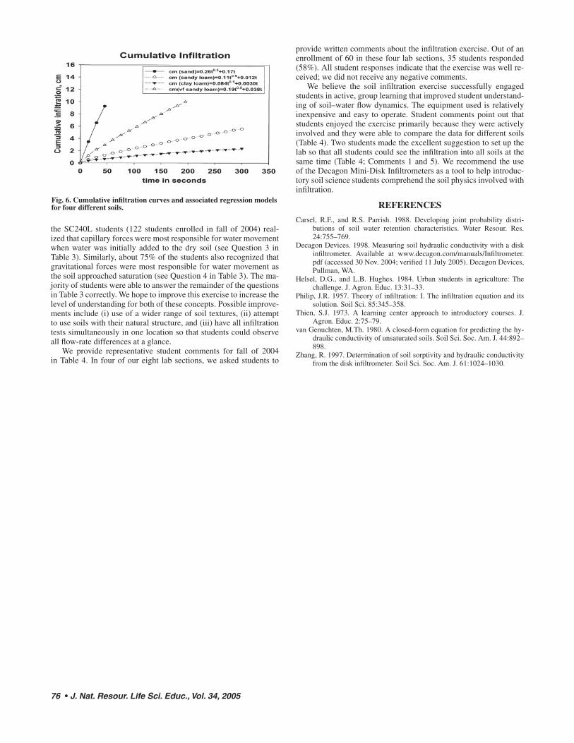
tion system onto a screen. We then discussed the resulting differenc-es for the soils. For example, we prompted the students to discuss what may have caused the Terry very fine sandy loam to have larger cumulative infiltration than the Bresser sandy loam (fine-loamy, mixed, superactive, mesic Aridic Argiustolls). We believed showing the results for all soils on the same graph allowed students to under-stand some of the infiltration physics.

After extracting the wetted soil in the Terry very fine sandy loam container, we had each student group observe the three-dimensional pattern of soil wetting. We pointed out the water movement was equidistant in every radial direction from the water source. We cued them to think of what forces would pull the water equally in all directions.

Even after showing the three-dimensional nature of wetting front and emphasizing the importance of capillary forces, about 75% of

Haplargids) (Table 2) after students completed the infiltration exer-cise. The Terry soil was the only soil in which we could remove the wetted soil intact. This showed the three-dimensional wetting and how the water had moved through the dry soil (see Fig. 4 and 5).

On the formal course evaluation for Introductory Soil Science Laboratory (SC240L) at the end of the Fall 2004 semester, we asked students in four out of eight lab sections (60 students) to provide anonymous written comments on the soil infiltration exercise. We plan to use this information to improve the exercise.

RESULTS AND DISCUSSION

After each student group finished the infiltration exercise, we projected one graph containing all SigmaPlot infiltration curves and associated regression analyses (Fig. 6) through a computer projec-

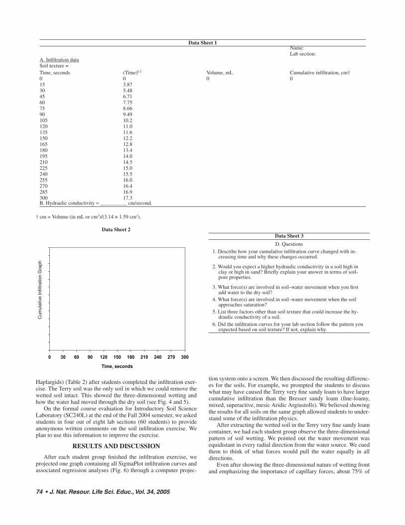
Data Sheet 1Name:Lab section:

A. Infiltration dataSoil texture = Time, seconds (Time)0.5 Volume, mL Cumulative infiltration, cm†0 0 0 015 3.8730 5.4845 6.7160 7.7575 8.6690 9.49105 10.2120 11.0135 11.6150 12.2165 12.8180 13.4195 14.0210 14.5225 15.0240 15.5255 16.0270 16.4285 16.9300 17.3B. Hydraulic conductivity = __________ cm/second.

C. Cumulative Infiltration Graph

Time, seconds

0 30 60 90 120 150 180 210 240 270 300

Cum

ulative Infiltration, cm

Data Sheet 2

Cum

ulat

ive

Infil

trat

ion

Gra

ph

† cm = Volume (in mL or cm3)/(3.14 × 1.59 cm2).

Data Sheet 3

D. Questions1. Describe how your cumulative infiltration curve changed with in-

creasing time and why these changes occurred.

2. Would you expect a higher hydraulic conductivity in a soil high in clay or high in sand? Briefly explain your answer in terms of soil-pore properties.

3. What force(s) are involved in soil–water movement when you first add water to the dry soil?

4. What force(s) are involved in soil–water movement when the soil approaches saturation?

5. List three factors other than soil texture that could increase the hy-draulic conductivity of a soil.

6. Did the infiltration curves for your lab section follow the pattern you expected based on soil texture? If not, explain why.

J. Nat. Resour. Life Sci. Educ., Vol. 34 2005 • 75

Table 4. Selected direct quotes, with original punctuation and spelling, from Introductory Soil Science Laboratory (SC240L) students from the fall of 2004 regarding the soil infiltration exercise.

1. I liked the infiltration lab, but it would have been nice to have been able to watch all the samples to be able to compare them.

2. The infiltration was good; it was good to actually see how different soils have different infiltration rates.

3. The infiltration was probably the best, because we learned the most from what we were doing.

4. I enjoyed the infiltration project. It was very interesting to see the differences between the different soils.

5. Infiltration lab was really good. It would have been nice to see the infiltration of water into other soils, but it was good to see the numbers.

6. I found that the infiltration exercise was fun and educational, and tied in to the lecture well. You should keep it in this course.

7. As for the new labs, infiltration was cool and it is good to know.

8. The infiltration lab was pretty fun. It was neat to dig out the infiltration front with the poop scoop and see its shape.

9. The infiltration lab was a very fun lab to do. It was my favorite lab that I did.

10. The new lab is very good; it is one of the most memorable.

11. Thought the lab with soil permeability was interesting and should be repeated.

12. The lab with perculations was very informative and fun.

13. The infiltration exercise was awesome. I did enjoy it.

14. The infiltration exercise I thought was a very good lab procedure and I feel that I learned a lot from it. You should use this lab procedure in the future.

15. I really liked the infiltration lab, it made a good point about how pore size affects H2O movement—it showed that what we learned in class really

does happen!!

16. The infiltration exercise seemed to be the most hands on and most involved in lab. Fun to put the information to good use.

Fig. 2. Securing the infiltrometer to pinch clamp and positioning it above the soil surface.

Fig. 3. Contacting the porous plate to the soil surface and initiating in-filtration

Fig. 5. Side view of the Terry very fine sandy loam wetting front after wetted soil is removed from the plastic container.

Fig. 4. Top view of the Terry very fine sandy loam wetting front after wetted soil is removed from the plastic container.

76 • J. Nat. Resour. Life Sci. Educ., Vol. 34, 2005

the SC240L students (122 students enrolled in fall of 2004) real-ized that capillary forces were most responsible for water movement when water was initially added to the dry soil (see Question 3 in Table 3). Similarly, about 75% of the students also recognized that gravitational forces were most responsible for water movement as the soil approached saturation (see Question 4 in Table 3). The ma-jority of students were able to answer the remainder of the questions in Table 3 correctly. We hope to improve this exercise to increase the level of understanding for both of these concepts. Possible improve-ments include (i) use of a wider range of soil textures, (ii) attempt to use soils with their natural structure, and (iii) have all infiltration tests simultaneously in one location so that students could observe all flow-rate differences at a glance.

We provide representative student comments for fall of 2004 in Table 4. In four of our eight lab sections, we asked students to

provide written comments about the infiltration exercise. Out of an enrollment of 60 in these four lab sections, 35 students responded (58%). All student responses indicate that the exercise was well re-ceived; we did not receive any negative comments.

We believe the soil infiltration exercise successfully engaged students in active, group learning that improved student understand-ing of soil–water flow dynamics. The equipment used is relatively inexpensive and easy to operate. Student comments point out that students enjoyed the exercise primarily because they were actively involved and they were able to compare the data for different soils (Table 4). Two students made the excellent suggestion to set up the lab so that all students could see the infiltration into all soils at the same time (Table 4; Comments 1 and 5). We recommend the use of the Decagon Mini-Disk Infiltrometers as a tool to help introduc-tory soil science students comprehend the soil physics involved with infiltration.

REFERENCES

Carsel, R.F., and R.S. Parrish. 1988. Developing joint probability distri-butions of soil water retention characteristics. Water Resour. Res. 24:755–769.

Decagon Devices. 1998. Measuring soil hydraulic conductivity with a disk infiltrometer. Available at www.decagon.com/manuals/Infiltrometer.pdf (accessed 30 Nov. 2004; verified 11 July 2005). Decagon Devices, Pullman, WA.

Helsel, D.G., and L.B. Hughes. 1984. Urban students in agriculture: The challenge. J. Agron. Educ. 13:31–33.

Philip, J.R. 1957. Theory of infiltration: I. The infiltration equation and its solution. Soil Sci. 85:345–358.

Thien, S.J. 1973. A learning center approach to introductory courses. J. Agron. Educ. 2:75–79.

van Genuchten, M.Th. 1980. A closed-form equation for predicting the hy-draulic conductivity of unsaturated soils. Soil Sci. Soc. Am. J. 44:892–898.

Zhang, R. 1997. Determination of soil sorptivity and hydraulic conductivity from the disk infiltrometer. Soil Sci. Soc. Am. J. 61:1024–1030.

Fig. 6. Cumulative infiltration curves and associated regression models for four different soils.