1

InfiltrationInfiltration

2

Purpose of infiltration modelsPurpose of infiltration models Irrigation planningIrrigation planning Drainage calculationsDrainage calculations Hydrological modelsHydrological models Soil erosion modelsSoil erosion models

3

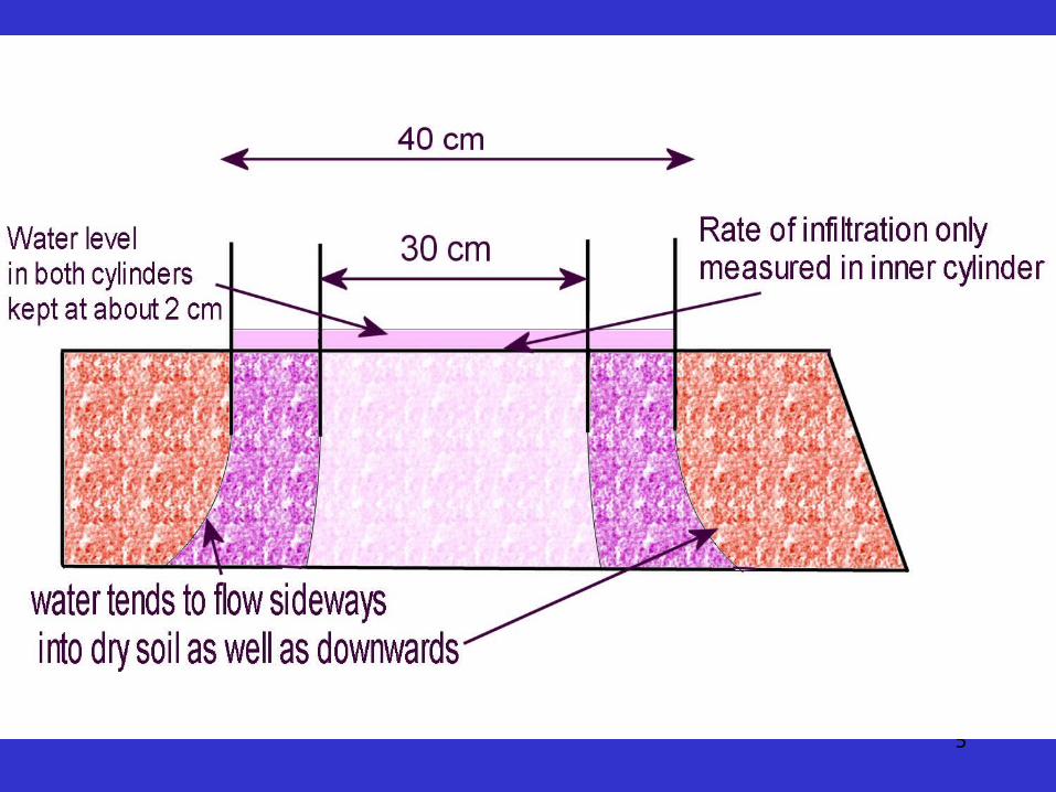
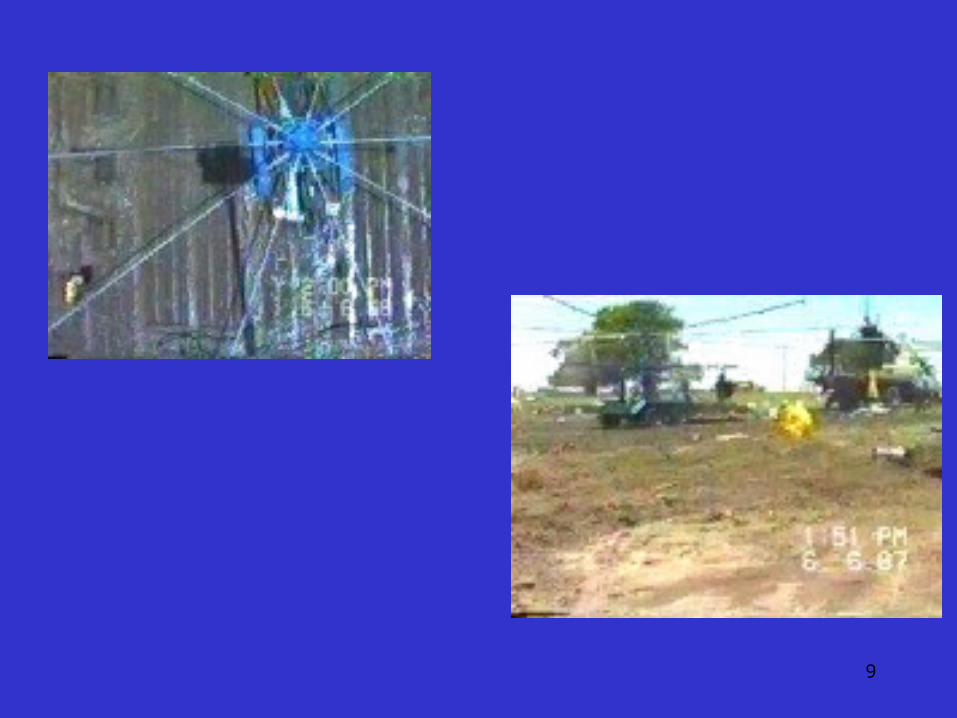
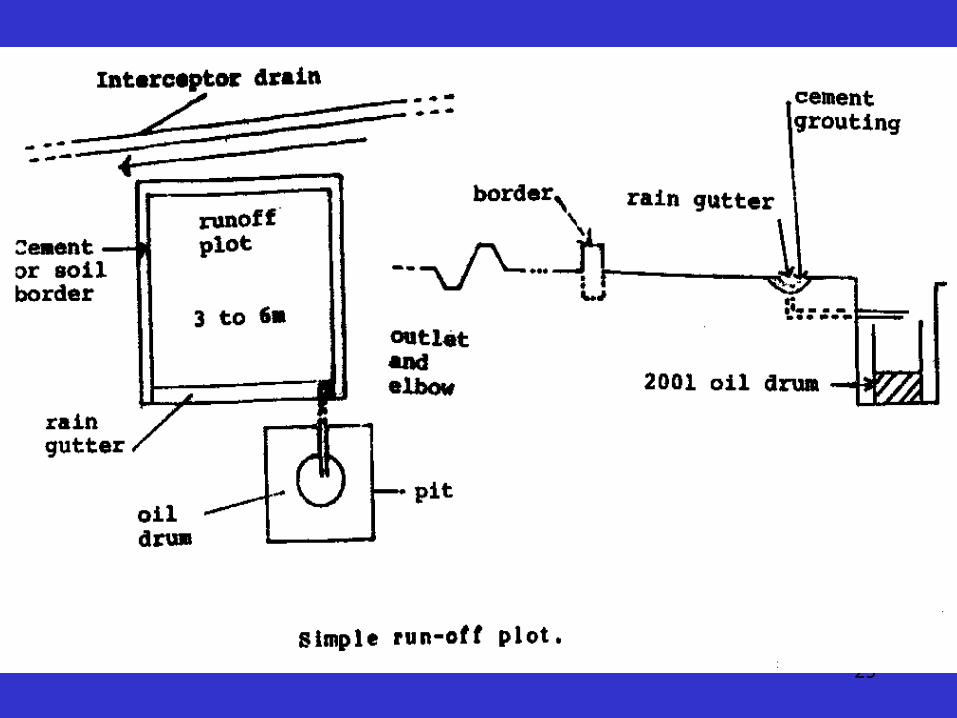
Measurement Measurement double ring method - gives values which are double ring method - gives values which are too high for soil erosion studies, so best usetoo high for soil erosion studies, so best use rainfall simulators for this purpose - but rainfall simulators for this purpose - but method is fine for surface irrigation designmethod is fine for surface irrigation design

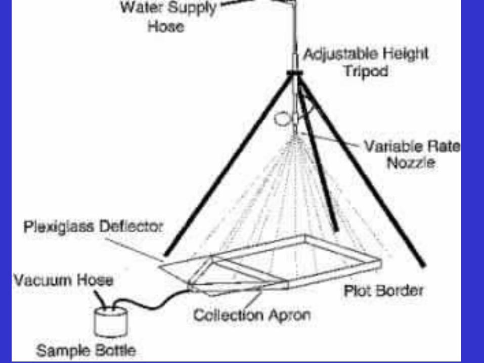
rainfall simulator (best for sprinkler irrigationrainfall simulator (best for sprinkler irrigation design and hydrological modelling)design and hydrological modelling)

4

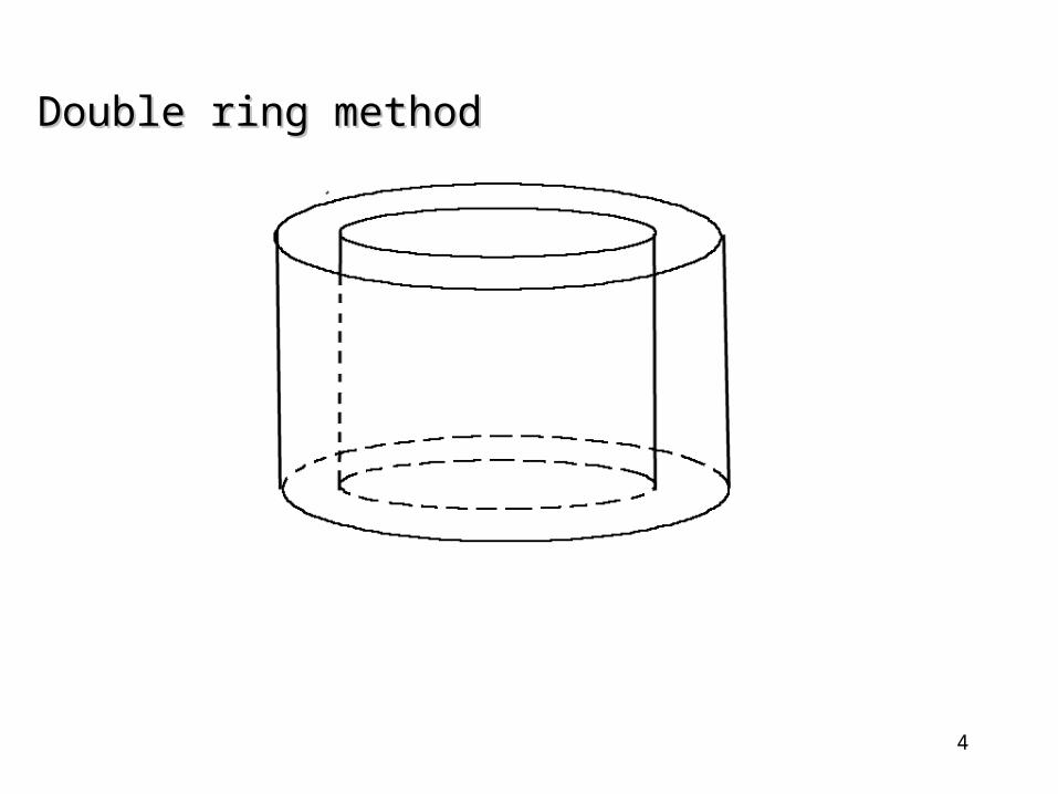
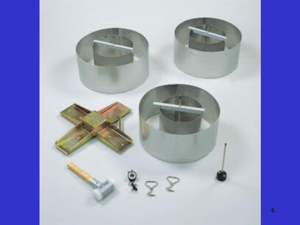
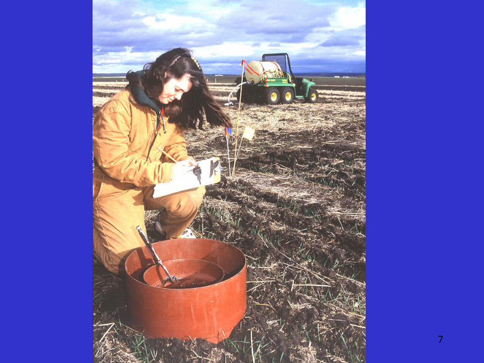
Double ring methodDouble ring method

5

6

7

8

9

10

ModelingModeling

Some workers have used texture, bulk density Some workers have used texture, bulk density (e.g.)(e.g.) to predict infiltration but reality is to predict infiltration but reality is complicated by complicated by e.g.e.g. roots, fauna, tillage roots, fauna, tillage system, system, etcetc. so be cautious with equations. so be cautious with equations

11

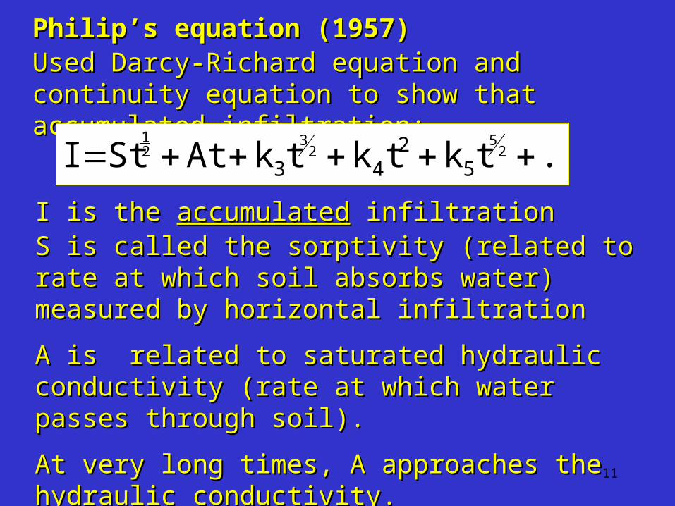
I is the I is the accumulatedaccumulated infiltration infiltrationS is called the sorptivity (related to rate at S is called the sorptivity (related to rate at which soil absorbs water) measured by which soil absorbs water) measured by horizontal infiltration horizontal infiltration

A is related to saturated hydraulic A is related to saturated hydraulic conductivity (rate at which water passes conductivity (rate at which water passes through soil).through soil).

At very long times, A approaches the At very long times, A approaches the hydraulic conductivity.hydraulic conductivity.

Philip’s equation (1957)Philip’s equation (1957)Used Darcy-Richard equation and continuity Used Darcy-Richard equation and continuity equation to show that accumulated infiltration:equation to show that accumulated infiltration:

...tktktkAtStI 25

23

21

52

43

12

ASt 21

21

dtdI

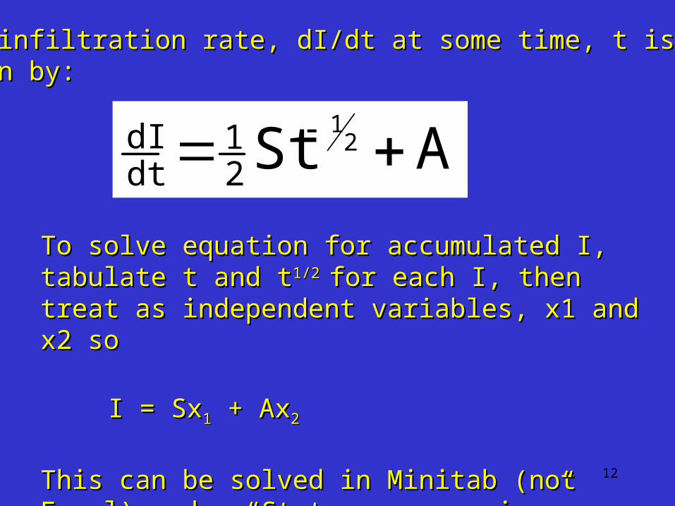
The infiltration rate, dI/dt at some time, t is The infiltration rate, dI/dt at some time, t is given by:given by:

To solve equation for accumulated I, tabulate To solve equation for accumulated I, tabulate t and tt and t1/2 1/2 for each I, then treat as independent for each I, then treat as independent variables, x1 and x2 sovariables, x1 and x2 so

I = SxI = Sx11 + Ax + Ax22

This can be solved in Minitab (not Excel) This can be solved in Minitab (not Excel) under “Stats - regression” (untick intercept under “Stats - regression” (untick intercept box)box)

13

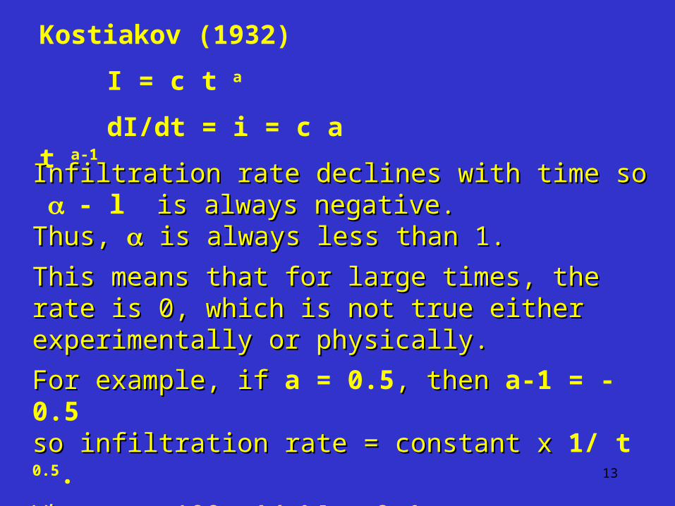
Kostiakov (1932)

I = c t a

dI/dt = i = c a t a-1

Infiltration rate declines with time soInfiltration rate declines with time so - l is is always negative.always negative.Thus, Thus, is always less than 1. is always less than 1.

This means that for large times, the rate is 0, This means that for large times, the rate is 0, which is not true either experimentally or which is not true either experimentally or physically. physically.

For example, if For example, if a = 0.5, , thenthen a-1 = - 0.5 so infiltration rate = constant xso infiltration rate = constant x 1/ t 0.5.

When t = 100,When t = 100, 1/t0.5 = 0.1. . When t=10000,When t=10000, 1/t 0.5 = = 0.01 0.01, , and so onand so on

14

To find To find aa and c, tabulate logarithms of I and t and c, tabulate logarithms of I and t in Excel. in Excel.

If y = log I and x = log t, and k=log c thenIf y = log I and x = log t, and k=log c theny = k + y = k + aax so plot y against x and plot the x so plot y against x and plot the curves and “Add Trendline” using the curves and “Add Trendline” using the “include equation” option. “include equation” option.

The slope of the line is The slope of the line is a a and the intercept is and the intercept is k from which you can calculate ck from which you can calculate c

15

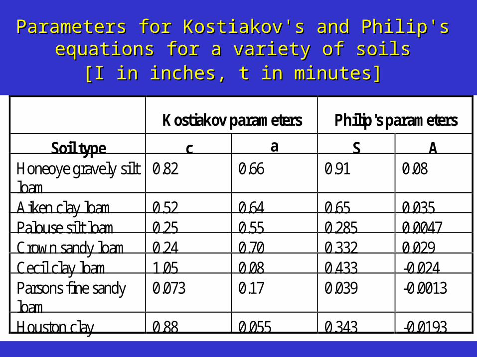
Kostiakov parameters Philip's parameters

Soil type c a S A Honeoye gravely siltloam

0.82 0.66 0.91 0.08

Aiken clay loam 0.52 0.64 0.65 0.035 Palouse silt loam 0.25 0.55 0.285 0.0047 Crown sandy loam 0.24 0.70 0.332 0.029 Cecil clay loam 1.05 0.08 0.433 -0.024 Parsons fine sandyloam

0.073 0.17 0.039 -0.0013

Houston clay 0.88 0.055 0.343 -0.0193

Parameters for Kostiakov's and Philip's Parameters for Kostiakov's and Philip's equations for a variety of soilsequations for a variety of soils

[I in inches, t in minutes][I in inches, t in minutes]

16

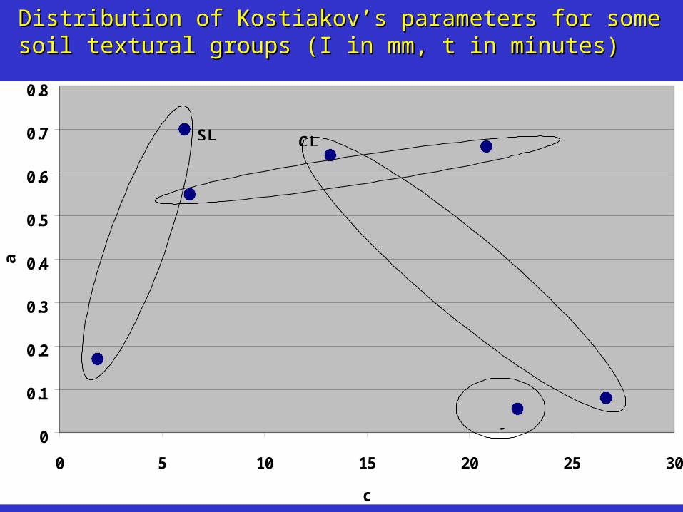
Distribution of Kostiakov’s parameters for some soil Distribution of Kostiakov’s parameters for some soil textural groups (I in mm, t in minutes)textural groups (I in mm, t in minutes)

0

0.1

0.2

0.3

0.4

0.5

0.6

0.7

0.8

0 5 10 15 20 25 30

c

a

ZL

ZL

CL

CL

Clay

SL

fSL

17

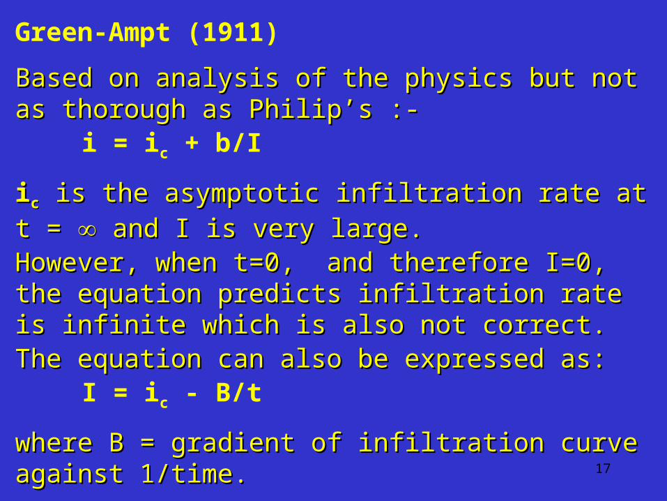
Green-Ampt (1911)

Based on analysis of the physics but not as Based on analysis of the physics but not as thorough as Philip’s :-thorough as Philip’s :-

i = ic + b/I

iicc is the asymptotic infiltration rate at t = is the asymptotic infiltration rate at t = and I and I is very large.is very large.However, when t=0, and therefore I=0, the However, when t=0, and therefore I=0, the equation predicts infiltration rate is infinite equation predicts infiltration rate is infinite which is also not correct. which is also not correct. The equation can also be expressed as:The equation can also be expressed as:

I = ic - B/t

where B = gradient of infiltration curve against where B = gradient of infiltration curve against 1/time.1/time.

18

To solve, plot I against 1/t and find the To solve, plot I against 1/t and find the slope and the interceptslope and the intercept

19

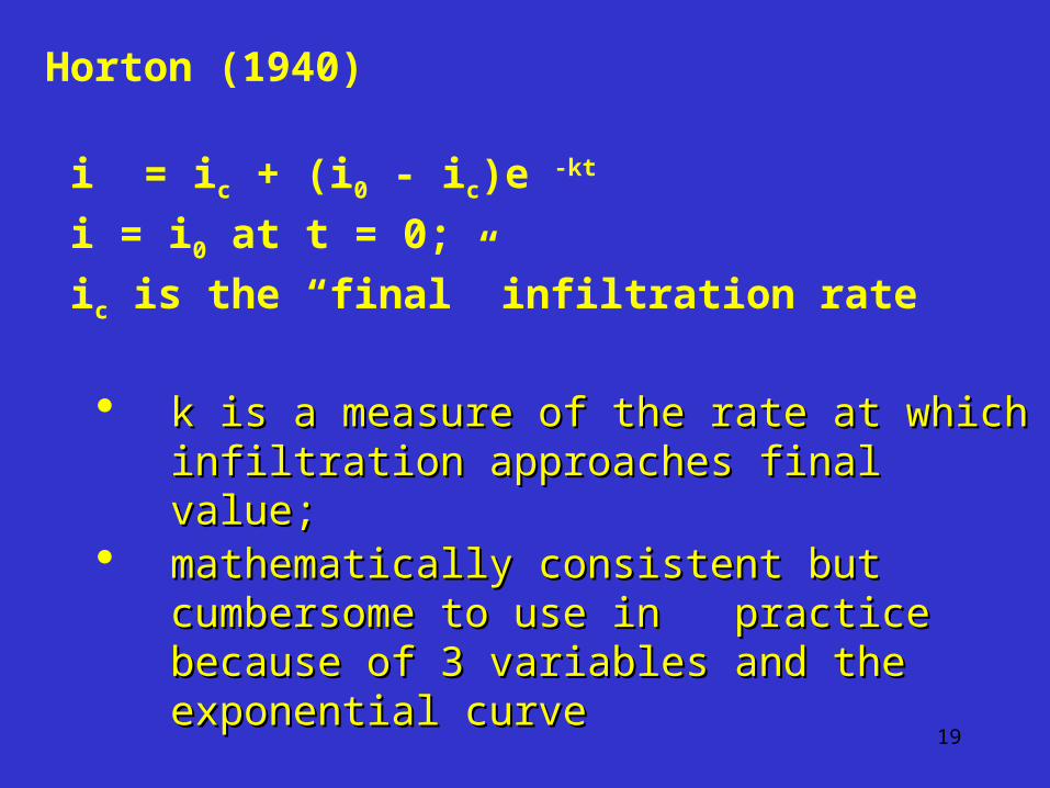
Horton (1940)

i = ic + (i0 - ic)e -kt

i = i0 at t = 0;

ic is the “final” infiltration rate

k is a measure of the rate at which k is a measure of the rate at which infiltration approaches final value;infiltration approaches final value;

mathematically consistent but mathematically consistent but cumbersome to use in practice because cumbersome to use in practice because of 3 variables and the exponential curveof 3 variables and the exponential curve

20

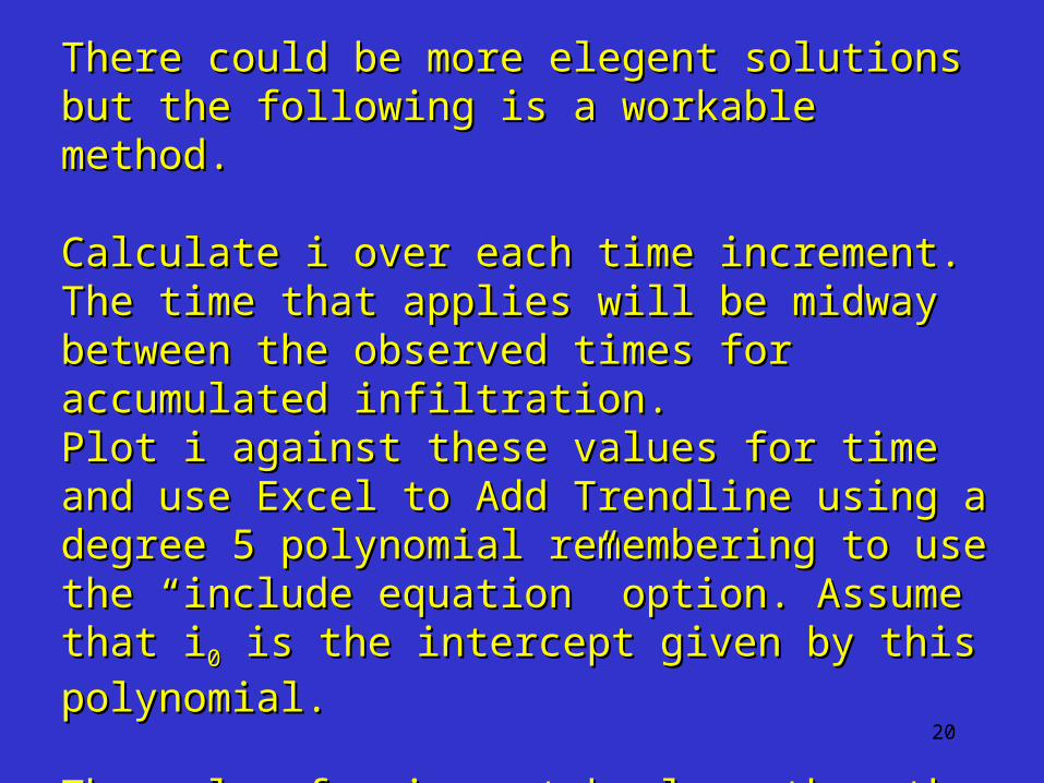
There could be more elegent solutions but There could be more elegent solutions but the following is a workable method.the following is a workable method.

Calculate i over each time increment. The Calculate i over each time increment. The time that applies will be midway between the time that applies will be midway between the observed times for accumulated infiltration. observed times for accumulated infiltration. Plot i against these values for time and use Plot i against these values for time and use Excel to Add Trendline using a degree 5 Excel to Add Trendline using a degree 5 polynomial remembering to use the “include polynomial remembering to use the “include equation” option. Assume that iequation” option. Assume that i00 is the is the intercept given by this polynomial.intercept given by this polynomial.

The value for iThe value for icc must be less than the final must be less than the final observed value. Set up a range of possible observed value. Set up a range of possible values from 0.5 x final value to 1.0 x final values from 0.5 x final value to 1.0 x final value.value.

21

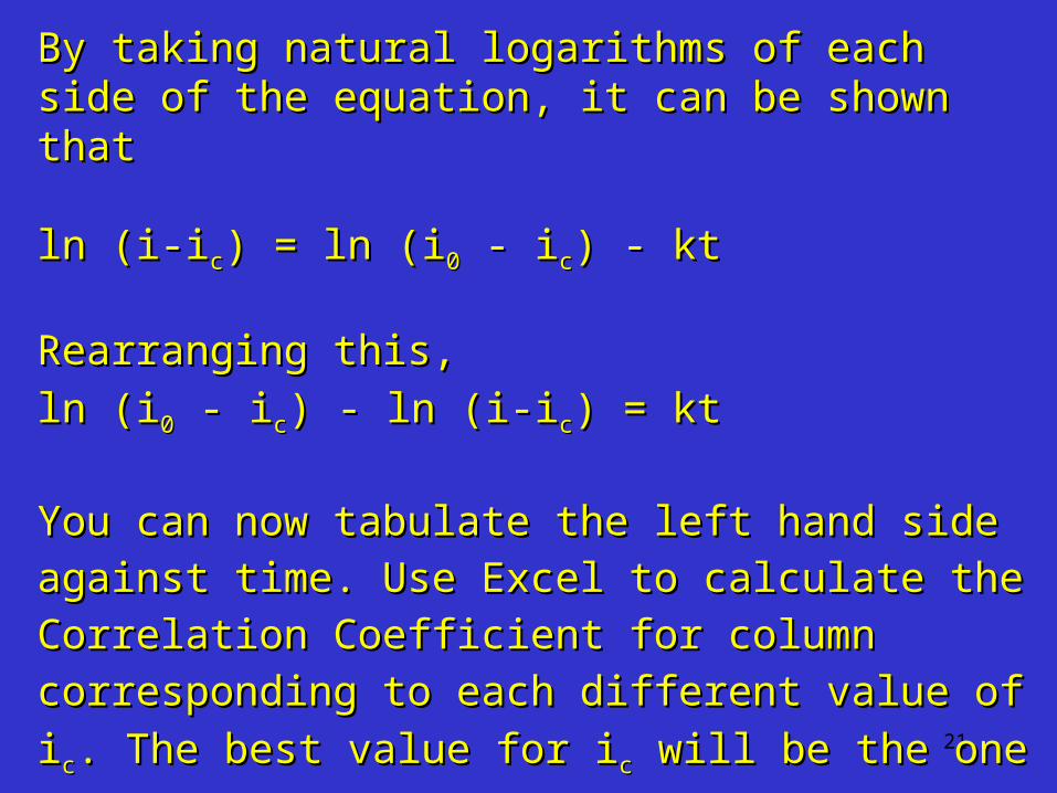
By taking natural logarithms of each side of the By taking natural logarithms of each side of the equation, it can be shown thatequation, it can be shown that

ln (i-iln (i-icc) = ln (i) = ln (i00 - i - icc) - kt) - kt

Rearranging this, Rearranging this, ln (iln (i00 - i - icc) - ln (i-i) - ln (i-icc) = kt) = kt

You can now tabulate the left hand side against You can now tabulate the left hand side against time. Use Excel to calculate the Correlation time. Use Excel to calculate the Correlation Coefficient for column corresponding to each Coefficient for column corresponding to each different value of idifferent value of icc. The best value for i. The best value for icc will be will be

the one with the highest correlation coefficient. the one with the highest correlation coefficient. Otherwise use programmes like SASOtherwise use programmes like SAS

22

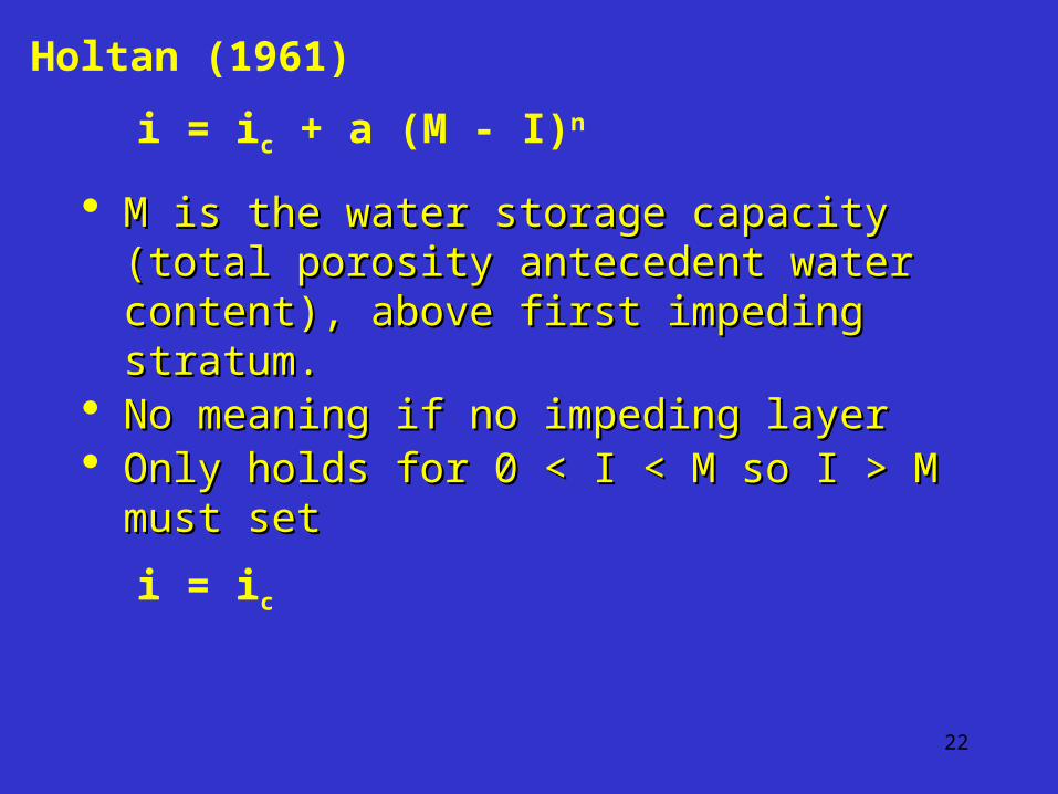
Holtan (1961)

i = ic + a (M - I)n

M is the water storage capacity (total M is the water storage capacity (total porosity antecedent water content), above porosity antecedent water content), above first impeding stratum. first impeding stratum.

No meaning if no impeding layerNo meaning if no impeding layer Only holds for 0 < I < M so I > M must set Only holds for 0 < I < M so I > M must set

i = ic

23

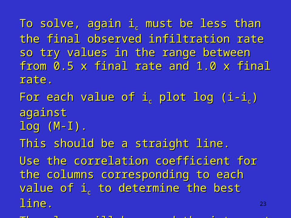
To solve, again iTo solve, again icc must be less than the final must be less than the final observed infiltration rate so try values in the observed infiltration rate so try values in the range between from 0.5 x final rate and 1.0 x range between from 0.5 x final rate and 1.0 x final rate.final rate.

For each value of iFor each value of icc plot log (i-i plot log (i-icc) against ) against log (M-I). log (M-I).

This should be a straight line. This should be a straight line.

Use the correlation coefficient for the Use the correlation coefficient for the columns corresponding to each value of icolumns corresponding to each value of icc to to determine the best line. determine the best line.

The slope will be n and the intercept will be The slope will be n and the intercept will be log a.log a.

24

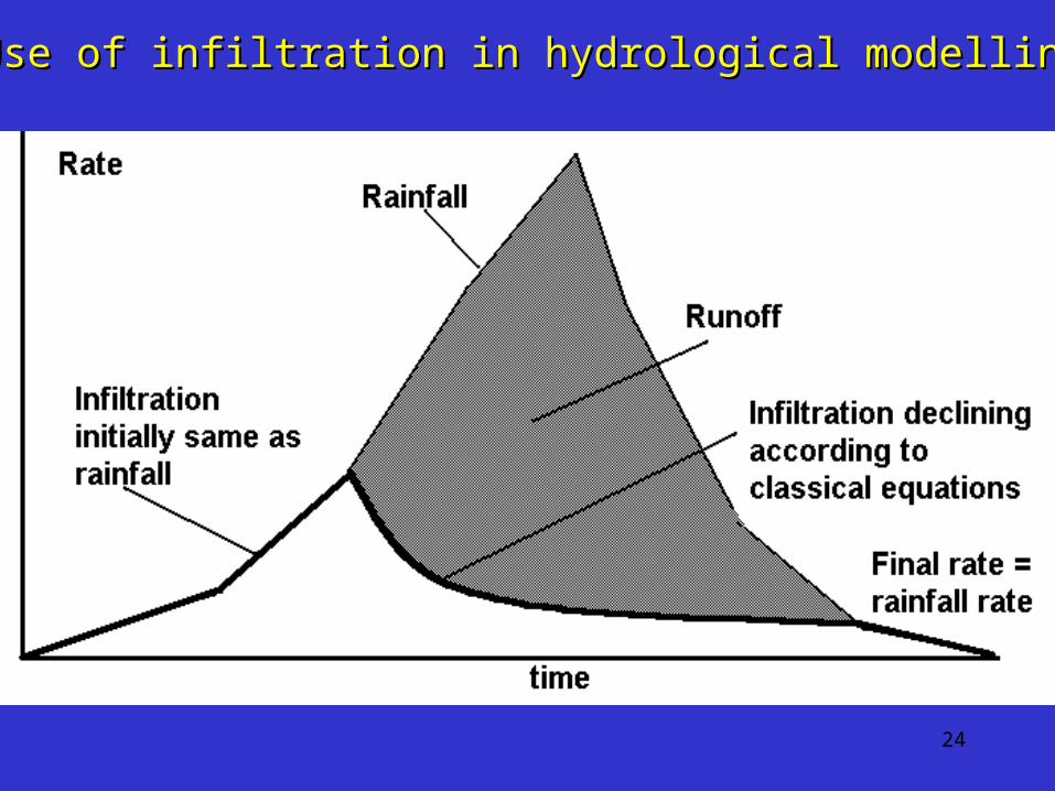
Use of infiltration in hydrological modellingUse of infiltration in hydrological modelling

25

26

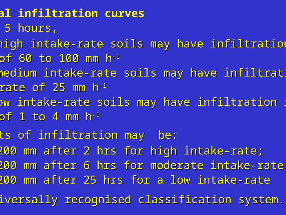
Typical infiltration curvesAfter 5 hours,After 5 hours,

high intake-rate soils may have infiltration ratehigh intake-rate soils may have infiltration rate of 60 to 100 mm hof 60 to 100 mm h-1-1

medium intake-rate soils may have infiltration medium intake-rate soils may have infiltration rate of 25 mm hrate of 25 mm h-1-1

low intake-rate soils may have infiltration ratelow intake-rate soils may have infiltration rate of 1 to 4 mm hof 1 to 4 mm h-1-1

Amounts of infiltration may be:Amounts of infiltration may be: 200 mm after 2 hrs for high intake-rate;200 mm after 2 hrs for high intake-rate; 200 mm after 6 hrs for moderate intake-rate;200 mm after 6 hrs for moderate intake-rate; 200 mm after 25 hrs for a low intake-rate 200 mm after 25 hrs for a low intake-rate

No universally recognised classification system.No universally recognised classification system.

27

0

10

20

30

40

50

60

70

80

90

1000 5

10 15 20 25 30 35 40 45 50 55 60 65 70 75 80 85 90 95

100

105

110

time (mins)

Infi

ltra

tion

(m

m)

1

2

3

4

5

6

7

8

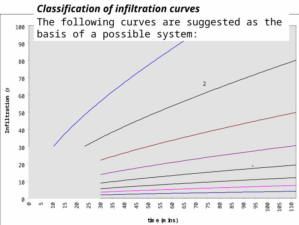
Classification of infiltration curvesThe following curves are suggested as the basis of a possible system:

28

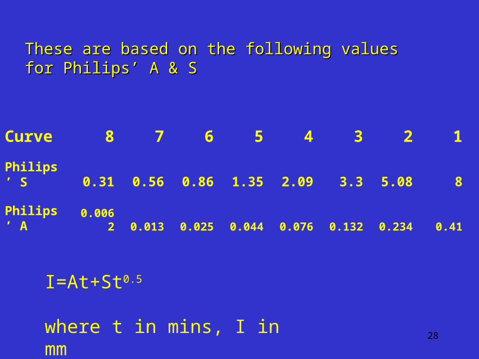
I=At+St0.5

where t in mins, I in mm

Curve 8 7 6 5 4 3 2 1

Philips’ S 0.31 0.56 0.86 1.35 2.09 3.3 5.08 8

Philips’ A

0.0062 0.013 0.025 0.044 0.076 0.132 0.234 0.41

These are based on the following values for These are based on the following values for Philips’ A & S Philips’ A & S

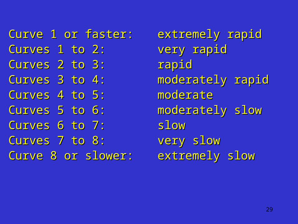
29

Curve 1 or faster: Curve 1 or faster: extremely rapidextremely rapidCurves 1 to 2: Curves 1 to 2: very rapidvery rapidCurves 2 to 3: Curves 2 to 3: rapidrapidCurves 3 to 4: Curves 3 to 4: moderately rapidmoderately rapidCurves 4 to 5: Curves 4 to 5: moderatemoderateCurves 5 to 6: Curves 5 to 6: moderately slowmoderately slowCurves 6 to 7: Curves 6 to 7: slowslowCurves 7 to 8: Curves 7 to 8: very slowvery slowCurve 8 or slower: Curve 8 or slower: extremely slowextremely slow

30

Infiltration rate

0

1

2

3

4

5

6

1 11 21 31 41 51 61

time (mins)

Infil

trat

ion

rate

(mm

/min

)

1

23

45

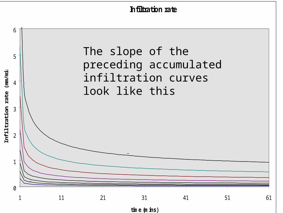
The slope of the preceding accumulated infiltration curves look like this

31

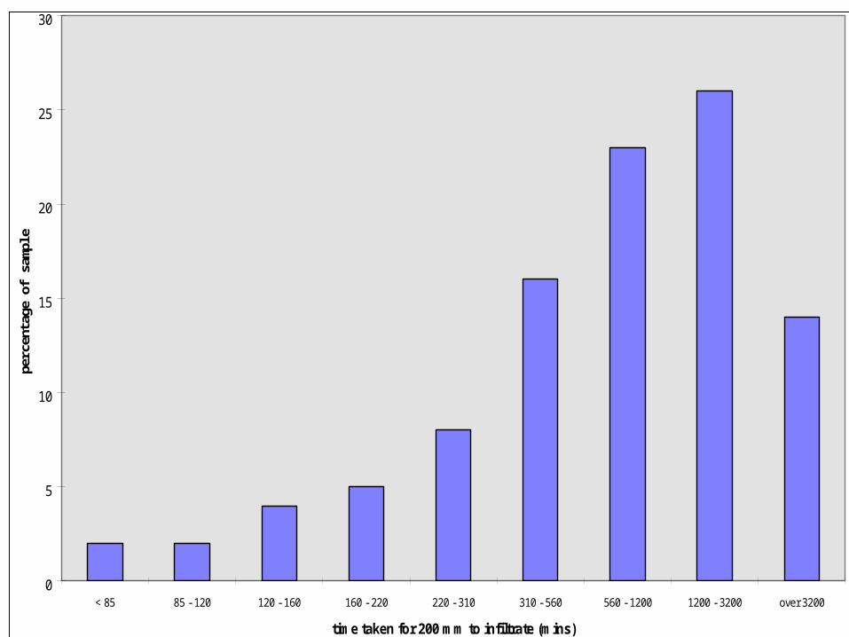
It should be noted that the distribution of It should be noted that the distribution of infiltration rates is log-normal and skewed. infiltration rates is log-normal and skewed.

The results of one experiment at a single site The results of one experiment at a single site are shown in the following diagram.are shown in the following diagram.

320

5

10

15

20

25

30

< 85 85 - 120 120 - 160 160 - 220 220 - 310 310 - 560 560 - 1200 1200 - 3200 over 3200

time taken for 200 mm to infiltrate (mins)

perc

enta

ge o

f sam

ple

33

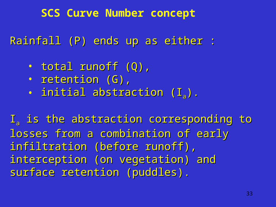
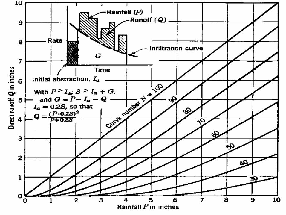
Rainfall (P) ends up as either :Rainfall (P) ends up as either :

• total runoff (Q), total runoff (Q), • retention (G), retention (G), • initial abstraction (Iinitial abstraction (Iaa). ).

SCS Curve Number concept

IIaa is the abstraction corresponding to losses is the abstraction corresponding to losses from a combination of early infiltration (before from a combination of early infiltration (before runoff), runoff), interception (on vegetation) and surface interception (on vegetation) and surface retention (puddles).retention (puddles).

34

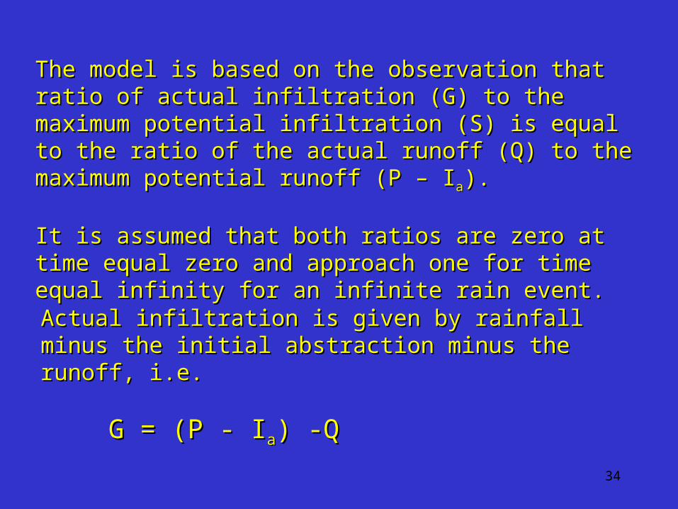
The model is based on the observation that ratio of The model is based on the observation that ratio of actual infiltration (G) to the maximum potential actual infiltration (G) to the maximum potential infiltration (S) is equal to the ratio of the actual infiltration (S) is equal to the ratio of the actual runoff (Q) to the maximum potential runoff (P – Irunoff (Q) to the maximum potential runoff (P – Iaa).).

It is assumed that both ratios are zero at time equal It is assumed that both ratios are zero at time equal zero and approach one for time equal infinity for an zero and approach one for time equal infinity for an infinite rain event. infinite rain event.

Actual infiltration is given by rainfall minus the initial Actual infiltration is given by rainfall minus the initial abstraction minus the runoff, i.e.abstraction minus the runoff, i.e.

G = (P - IG = (P - Iaa) -Q) -Q

35

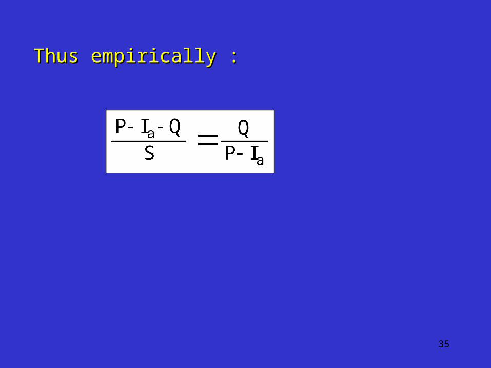
Thus empirically : Thus empirically :

36

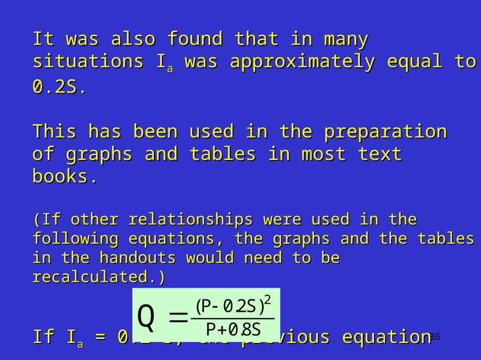
It was also found that in many situations IIt was also found that in many situations Iaa was was approximately equal to 0.2S. approximately equal to 0.2S.

This has been used in the preparation of This has been used in the preparation of graphs and tables in most text books. graphs and tables in most text books.

(If other relationships were used in the following (If other relationships were used in the following equations, the graphs and the tables in the handouts equations, the graphs and the tables in the handouts would need to be recalculated.)would need to be recalculated.)

If IIf Iaa = 0.2 S, the previous equation becomes :- = 0.2 S, the previous equation becomes :-

S8.0P)S2.0P( 2

Q

37

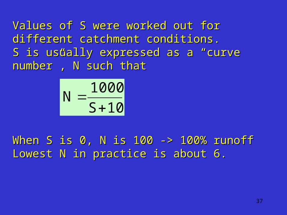
Values of S were worked out for different Values of S were worked out for different catchment conditions. catchment conditions. S is usually expressed as a “curve S is usually expressed as a “curve number”, N such thatnumber”, N such that

10S

1000N

When S is 0, N is 100 -> 100% runoffWhen S is 0, N is 100 -> 100% runoffLowest N in practice is about 6.Lowest N in practice is about 6.

38

39

see handout for tables to calculate Nsee handout for tables to calculate N

40

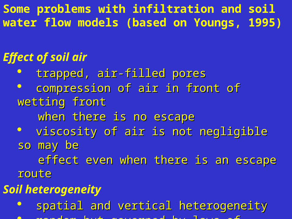
Some problems with infiltration and soil water flow models (based on Youngs, 1995)

Effect of soil air trapped, air-filled pores trapped, air-filled pores compression of air in front of wetting frontcompression of air in front of wetting front when there is no escape when there is no escape viscosity of air is not negligible so may beviscosity of air is not negligible so may be effect even when there is an escape route effect even when there is an escape route

Soil heterogeneity spatial and vertical heterogeneity spatial and vertical heterogeneity random but governed by laws of probabilityrandom but governed by laws of probability fingering/instability when less permeable > fingering/instability when less permeable > more permeable more permeable

41

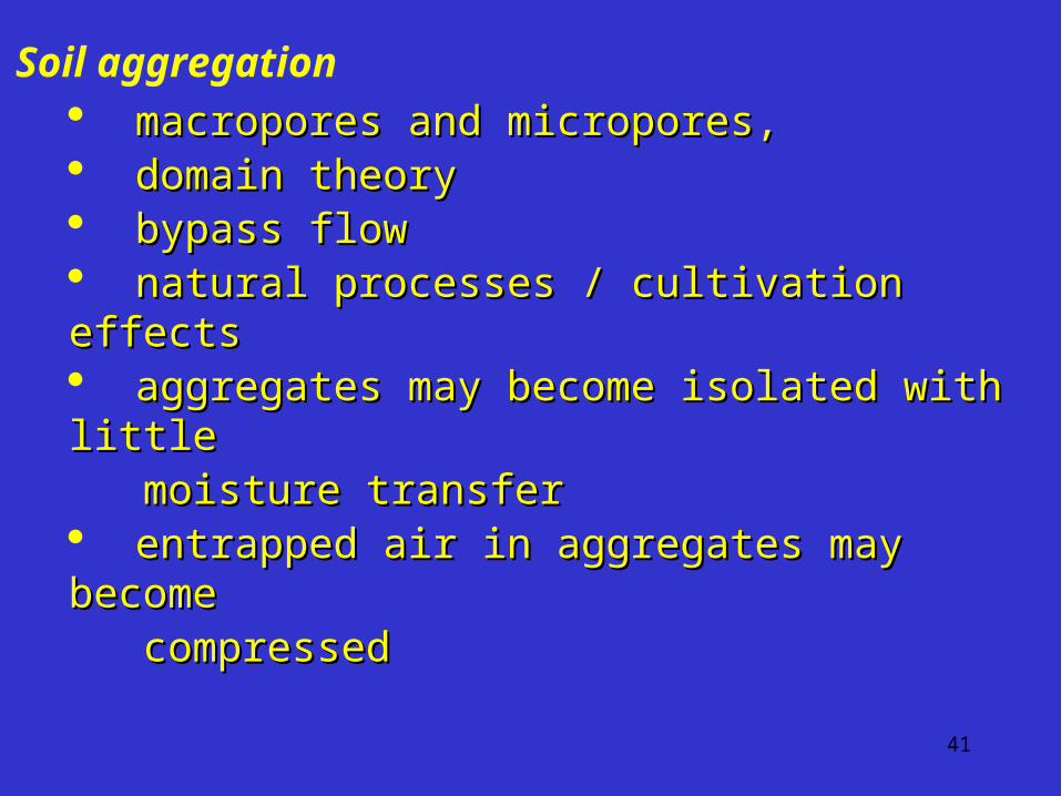
Soil aggregation macropores and micropores, macropores and micropores, domain theory domain theory bypass flow bypass flow natural processes / cultivation effects natural processes / cultivation effects aggregates may become isolated with littleaggregates may become isolated with little moisture transfer moisture transfer entrapped air in aggregates may becomeentrapped air in aggregates may become compressed compressed

42

Soil instabilityStructural breakdown and shrinking/swelling cause Structural breakdown and shrinking/swelling cause time dependent soil physical properties time dependent soil physical properties

43

Non-Darcian flow Soil water may not behave as classical fluid, Soil water may not behave as classical fluid, especially where there are electricallyespecially where there are electrically charged soil colloids;charged soil colloids;

Reynolds's number is used to predict type of Reynolds's number is used to predict type of flowflow

(turbulent, laminar). R is a function of (turbulent, laminar). R is a function of dimensions dimensions

of flow channel/pipe, viscosity, velocity. of flow channel/pipe, viscosity, velocity. Darcy's law fails at R>1, which it is duringDarcy's law fails at R>1, which it is during infiltration;infiltration;

Swelling / shrinking means that the frame ofSwelling / shrinking means that the frame of reference is moving! Geometry (shape) of reference is moving! Geometry (shape) of

structure is not constant swelling is not uniform structure is not constant swelling is not uniform in all directionsin all directions

44

Clay particles in suspension also move

In clay soils, part of the overburden is transmitted to the soil water- has to be allowed for in equations, proportion depends on the moisture content

45

Non-isothermal flow Theory assumes isothermal conditions but Theory assumes isothermal conditions but there there are thermal gradients near the surface and the are thermal gradients near the surface and the heat of wetting generated at the wetting front.heat of wetting generated at the wetting front.

Hysteresis• Hysteresis can be incorporated but diffusivity Hysteresis can be incorporated but diffusivity becomes discontinuous which makes analysis becomes discontinuous which makes analysis more more difficult.difficult.

46

Anisotropy

Solutions assume isotropic media - not true in Solutions assume isotropic media - not true in real soilsreal soils

Conductivity in horizontal direction may be Conductivity in horizontal direction may be different (usually slower) from the verticaldifferent (usually slower) from the vertical directiondirection

Anisotropic because of cracks, worm holes, etc.Anisotropic because of cracks, worm holes, etc.

47

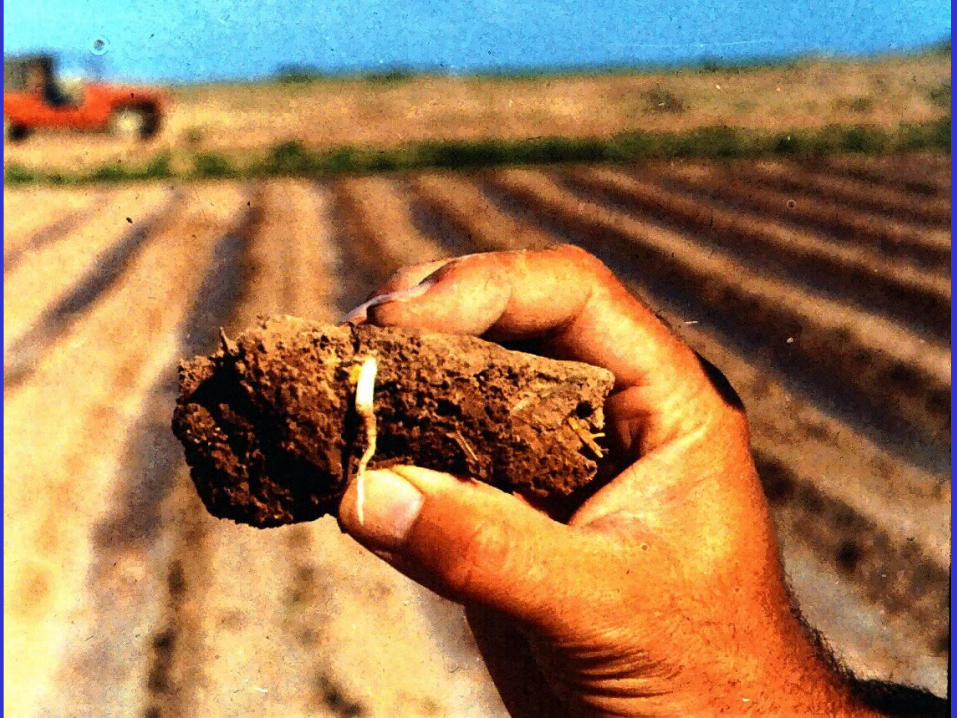
Effects of structureStructure has a great effect on infiltration. Structure has a great effect on infiltration.

For loam, range can be from 1.5 mm hFor loam, range can be from 1.5 mm h-1-1 for for massive structure to 150 mm hmassive structure to 150 mm h-1-1.for well .for well structured. structured.

Improved structure e.g. by roots and Improved structure e.g. by roots and infiltration will increase, runoff will decrease, infiltration will increase, runoff will decrease, erosion will decrease.erosion will decrease.

48

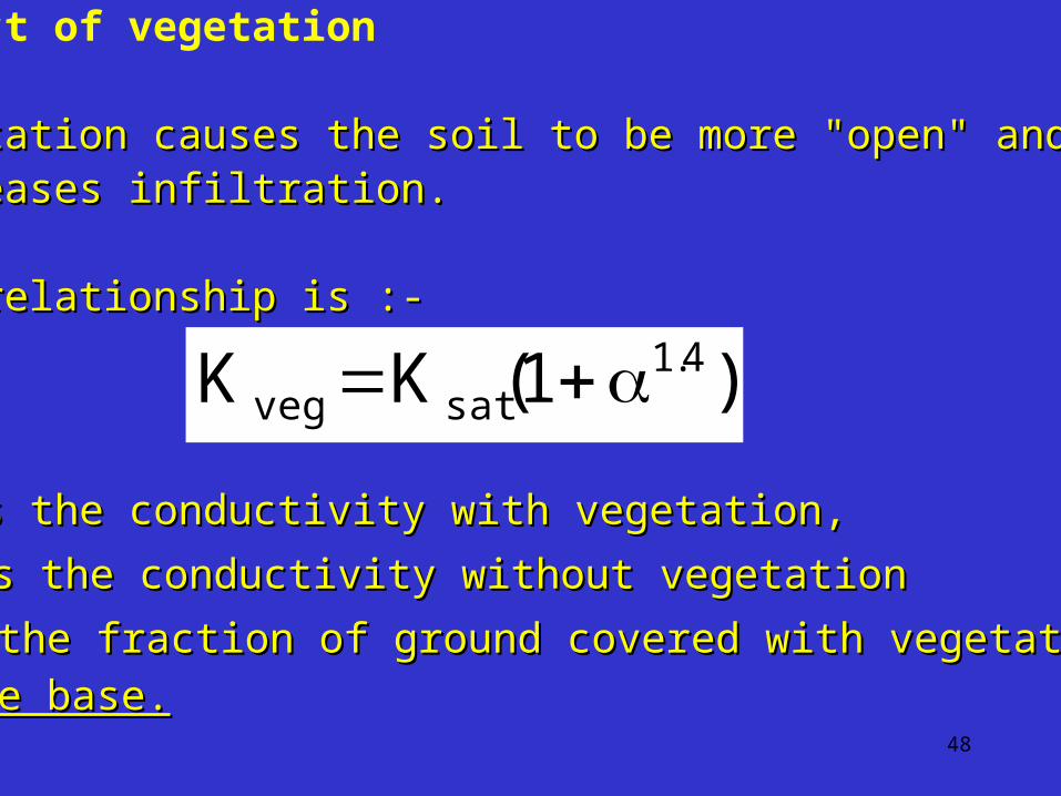
Effect of vegetation

Vegetation causes the soil to be more "open" and Vegetation causes the soil to be more "open" and increases infiltration. increases infiltration.

One relationship is :-One relationship is :-

)1(KK 4.1satveg

Kveg is the conductivity with vegetation, is the conductivity with vegetation,

Ksat is the conductivity without vegetationis the conductivity without vegetation

a is the fraction of ground covered with vegetation is the fraction of ground covered with vegetation at the base.at the base.

49

Alteration

For water harvesting, sometimes infiltration needs to be reduced (covered in 556 - Water Harvesting and Use of Chemicals)

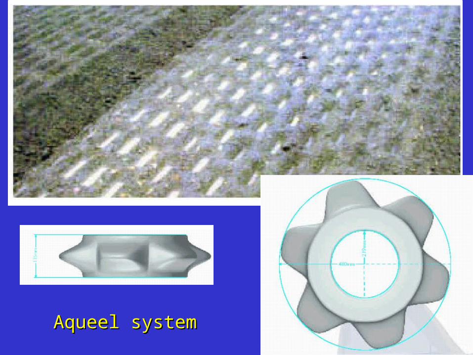
50Aqueel systemAqueel system

51

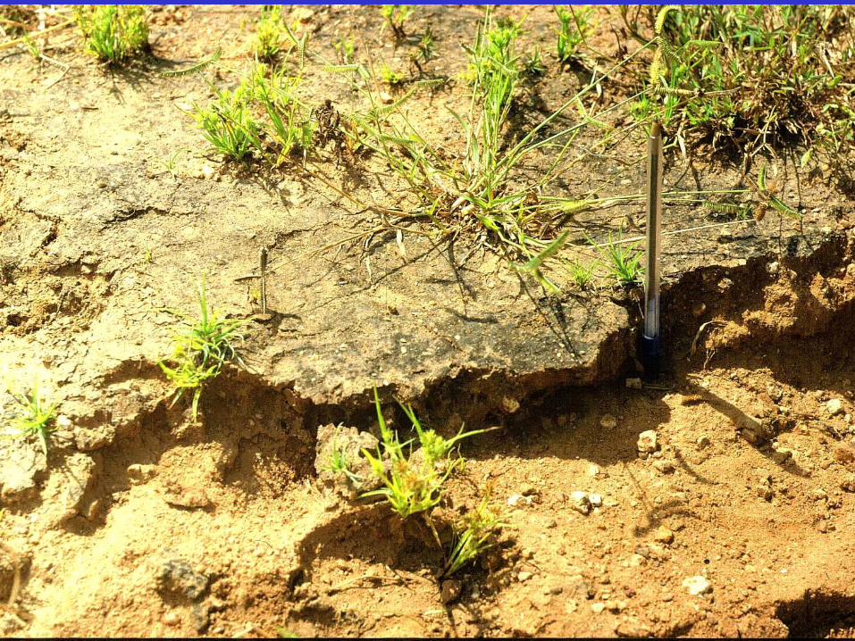
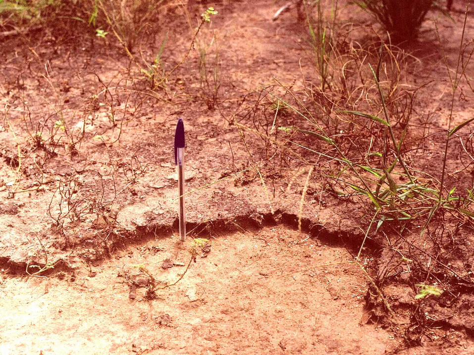
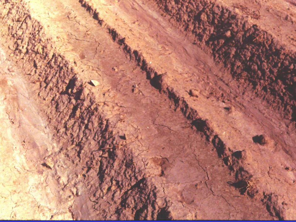
Crusts and capping

Caps caused by intense rain on bare soil, especially if low OM and/or high silt content.

Crustability decreases with increasing contents of clay and OM.

Crusts can reduce infiltration by a factor of 10.

Tall vegetation with no ground cover not only increases detachment because of drop sizes but alsosurface sealing.

52

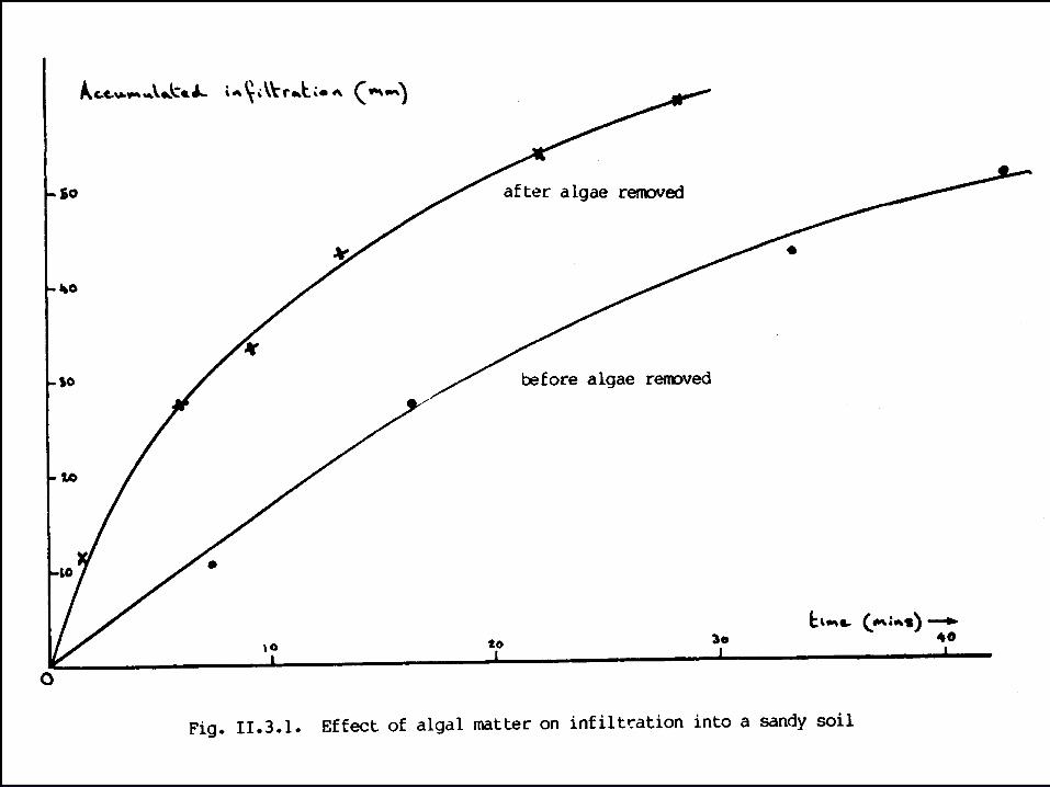
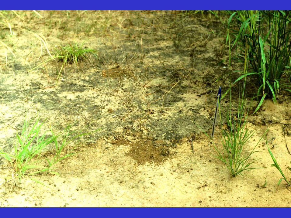
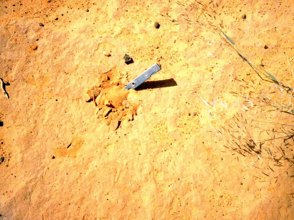
Algaemats of intertwined filamentous blue-green mats of intertwined filamentous blue-green algae can also reduce infiltration and hence algae can also reduce infiltration and hence contribute to soil erosioncontribute to soil erosion

algae samples taken from near Dilling in South algae samples taken from near Dilling in South Kordofan were predominantly Kordofan were predominantly Lyngbya Lyngbya spp. spp. and and MicrocoleusMicrocoleus spp spp

53

54

55

56

57

58

59