inferring interwell connectivity in a reservoir from

20 PETROVIETNAM - JOURNAL VOL 10/2020

PETROLEUM EXPLORATION & PRODUCTION

1. Introduction

Numerous studies on inferring interwell connectiv-ity in a waterflood have been carried out. Some of these studies used statistical techniques that are very different

INFERRING INTERWELL CONNECTIVITY IN A RESERVOIR FROM BOTTOMHOLE PRESSURE FLUCTUATIONS OF HYDRAULICALLY FRACTURED VERTICAL WELLS, HORIZONTAL WELLS, AND MIXED WELLBORE CONDITIONSDinh Viet Anh1, Djebbar Tiab2

1PetroVietnam Exploration Production Corporation2University of OklahomaEmail: [email protected]; [email protected]://doi.org/10.47800/PVJ.2020.10-03

from the approach used in this study. Albertoni and Lake developed a technique that calculates the fraction of flow caused by each of the injectors in a producer [1, 2]. This method uses a constrained Multivariate Linear Regression (MLR) model similar to the model proposed by Refunjol [3]. The model introduced by Albertoni and Lake, however, considered only the effect of injectors on producers, not producers on producers. Albertoni and Lake also intro-

Summary

A technique using interwell connectivity is proposed to characterise complex reservoir systems and provide highly detailed information about permeability trends, channels, and barriers in a reservoir. The technique, which uses constrained multivariate linear regression analysis and pseudosteady state solutions of pressure distribution in a closed system, requires a system of signal (or active) wells and response (or observation) wells. Signal wells and response wells can be either producers or injectors. The response well can also be either flowing or shut in. In this study, for consistency, waterflood systems are used where the signal wells are injectors, and the response wells are producers. Different borehole conditions, such as hydraulically fractured vertical wells, horizontal wells, and mixed borehole conditions, are considered in this paper.

Multivariate linear regression analysis was used to determine interwell connectivity coefficients from bottomhole pressure data. Pseudosteady state solutions for a vertical well, a well with fully penetrating vertical fractures, and a horizontal well in a closed rectangular reservoir were used to calculate the relative interwell permeability. The results were then used to obtain information on reservoir anisotropy, high-permeability channels, and transmissibility barriers. The cases of hydraulically fractured wells with different fracture half-lengths, horizontal wells with different lateral section lengths, and different lateral directions are also considered. Different synthetic reservoir simulation models are analysed, including homogeneous reservoirs, anisotropic reservoirs, high-permeability-channel reservoirs, partially sealing barriers, and sealing barriers.

The main conclusions drawn from this study include: (a) The interwell connectivity determination technique using bottomhole pressure fluctuations can be applied to waterflooded reservoirs that are being depleted by a combination of wells (e.g. hydraulically fractured vertical wells and horizontal wells); (b) Wellbore conditions at the observations wells do not affect interwell connectivity results; and (c) The complex pressure distribution caused by a horizontal well or a hydraulically fractured vertical well can be diagnosed using the pseudosteady state solution and, thus, its connectivity with other wells can be interpreted.

Key words: Interwell connectivity, bottomhole pressure fluctuations, waterflooding, vertical wells, horizontal wells, hydraulically fractured wells.

Date of receipt: 12/10/2020. Date of review and editing: 12 - 14/10/2020. Date of approval: 15/10/2020.

PETROVIETNAM JOURNALVolume 10/2020, p. 20 - 40ISSN 2615-9902

This article was presented at SPE Production and Operations Symposium and licensed by SPE (License ID: 1068761-1) to republish full paper in Petrovietnam Journal

21PETROVIETNAM - JOURNAL VOL 10/2020

PETROVIETNAM

duced the concepts and uses of diffusivity filters to account for the time lag and attenuation that occur between the stimulus (injection) and the response (production). The procedures were proven effective for synthetic reservoir models, as well as real water flood fields. Yousef et al. introduced a capacitance model in which a nonlinear signal processing model was used [4, 5]. Compared to Albertoni and Lake’s model which was a steady-state (purely resistive) one, the capacitance model included both capaci-tance (compressibility) and resistivity (transmissibil-ity) effects. The model used flow rate data and could include shut-in periods and bottom hole pressures (if available).

Dinh and Tiab [6 - 9] used a similar approach as Albertoni and Lake [1, 2], however, bottom hole pressure data were used instead of flow rate data. Some constraints were applied to the flow rates such as constant production rate at every producer and constant total injection rate. Using bottom hole pressure data offers several advantages: (a) diffusiv-ity filters are not needed, (b) minimal data is required and (c) flexible plan to collect data. All of the stud-ies above only considered fully penetrating vertical wells. Dinh and Tiab only considered reservoirs with vertical wells without any hydraulic fractures or hori-zontal wells [6 - 9].

In this study, bottomhole pressure fluctua-tions were used to determine the interwell con-nectivity in a waterflood where horizontal wells, hydraulically fractured vertical wells or both are present. MLR model was used to determine the interwell connectivity coefficients from bottom-hole pressure data. For the case of hydraulically fractured vertical wells, a late time solution for a well with a fully penetrating vertical fracture in a closed rectangular reservoir was used to calculate the influence functions and the relative interwell permeabilities. The case where the fractures are of different fracture half-lengths is also consid-ered. Similarly, for the horizontal well cases, the late time solution for a horizontal well in a closed rectangular reservoir was used to calculate the in-fluence functions and the relative interwell perme-abilities. The cases in which the reservoir contains horizontal wells of different lengths and different directions were also considered. In order to quan-tify the effect of observation wells on the interwell

connectivity coefficients, the case of different injector well lengths and unchanged producer well lengths was analysed. Results for different cases such as all wells are horizontal along the x-direction, along both x- and y-directions and different horizontal well lengths are provided.

This study also provides the results for different cases where mixed wellbore conditions are present. 5 injector and 4 pro-ducer synthetic reservoirs containing hydraulic fractures and vertical wells, horizontal and vertical wells or all three types of wellbore conditions are used in the analysis. The results were then used to obtain information on reservoir anisotropy, high permeability channels and transmissibility barriers. Different synthetic reservoir models were analysed including homoge-neous, anisotropic reservoirs, reservoirs with high permeability channel, partially sealing barrier and sealing barrier.

2. Analytical model and calculation approach

Previous studies have developed a novel technique to determine interwell connectivity from bottom hole pressure fluctuation data. This study extends the application of the tech-nique to hydraulically fractured, horizontal wells and mixed wellbore conditions. The technique was described in detail by Dinh and Tiab [6 - 9]. Key equations and definitions of dimen-sionless variables below are used throughout this study.

2.1. Dimensionless variable

Considering a multi-well system with producers or injectors and initial pressure pi, the solution for pressure distribution due to a fully penetrated vertical well in a close rectangular reservoir is as follows [10, 11]:

Where the dimensionless variables are defined in field units as follows:

ai is the influence function equivalent to the dimensionless pressure for the case of a single well in a bounded reservoir pro-duced at a constant rate. Assuming tsDA = 0, the influence func-tion is given as:

(1)

(2)

(3)

(4)

(5)

[ ]( )∑=

−=welln

isDADAeDeDiwDiwDDDiiDDADDD ttyxyxyxaqtyxp

1,,, ,,,,,,),,(

AxxD =

AyyD =

AxxD =

AyyD =

( )( )tyxppBq

khp iniref

D ,,2.141

−=µ

Ackttt

DAµφ

0002637.0=

( )( )tyxppBq

khp iniref

D ,,2.141

−=µ

Ackttt

DAµφ

0002637.0=



Equation 6 is valid for pseudosteady state flow and can be rewritten as below:

Equation 7 is the pressure response at point (xD, yD) due to a well n at (xwDn, ywDn) in a homogeneous closed rectangular reservoir. The influence function (an) can be different for different wellbore conditions as well as flow regimes (horizontal well, partial penetrating verti-cal well, fractured vertical well, etc.).

2.2. Shape factor calculation

Shape factors are used to calculate pressure at wells at different locations in a reservoir of a certain shape. Letting CA denote the shape factor, we have the well known shape factor equation:

with L = rw, Lxf and Lh/2 for vertical well, vertically fractured well and horizontal well respectively and γ is Euler’s constant (γ = 0.5772…)

Thus, the shape factor can be calculated using Equation 9 [12]:

Where the L term in the definitions of dimension-less quantities is L = Lxf which is the fracture half-length.

2.3. Influence function

2.3.1. Hydraulically fractured well

For a hydraulically fractured well, for simplicity, the late time solution for a uniform flux fracture in

a closed rectangular reservoir provided by Ozkan was used [13]. The influence function for hydraulically fractured well becomes:

Where the G-function is:

For the case of infinite conductivity fractures, the dimen-sionless pressure can be obtained by evaluating the above equation at xD = 0.732 [14].

2.3.2. Horizontal wells

The pressure distribution equation for a horizontal well in a closed rectangular reservoir is [13]:

pDh = ah = pDf + F1

Where

Where 222222/ eDD xkLnb ππ += and the L term in the dimen-

sionless definition is the horizontal well half-length L = Lh/2, and zD = z/h and LD = 1/hD = L/2h. xwD and ywD are at the mid-point of the well length for the uniform flux horizontal well case. For the infinite conductivity horizontal well case, Ozkan showed that the point xD = 0.732 used to calculate pressure distribution for an infinite conductivity fracture can also be used for an infinite conductivity horizontal well [13]. The term F1 can be rewritten as follows:

(6)

(7)

(8)

(9)

( )( ) ( )

( ) ( )

( ) ( )

( ) ( )��

�

��

� +−++−+

��

�

��

� +−++++

��

�

��

� ++++−+

��

�

��

� +++++= ∑ ∑

∞

−∞=

∞

−∞=

DA

eDiwDDeDiwDD

DA

eDiwDDeDiwDD

DA

eDiwDDeDiwDD

m n DA

eDiwDDeDiwDD

DAeDeDiwDiwDDDi

tmyyynxxx

E

tmyyynxxx

E

tmyyynxxx

E

tmyyynxxx

E

tyxyxyxa

422

422

422

422

21

,,,,,,

2,

2,

1

2,

2,

1

2,

2,

1

2

,

2

,1

,,

( ) [ ]∑=

=−welln

inADeDeDwDnwDnDDnini qtyxyxyxa

khByxpp

1,,,,,,2., µ

2

4ln5.02LCe

AtpA

DAwD γπ +=

( ) ��

�� +−=

γπ

eLALogptExpC wDDAA 2

424

( )kyyyxGxx

kxx

kx

kk

x

yyy

yy

xy

tp

DwDeDeDk eD

D

eD

wD

eD

eD

eD

wDD

eD

D

eD

eDDADf

,,,,coscos1sin12

23122

12

2

22

∑∞

=��

��

��

��

��

��

�+

��

��

� ++−+=

ππππ

ππ

( )

��

��

�

��

��

� +−+��

��

� −−

=

eD

eD

eD

wDDeD

eD

wDDeD

DwDeDeD

xyk

xyyyk

xyyy

k

kyyyxG

π

ππ

sinh

coshcosh

),,,,(

( ) ( )

( )

( ) ( )

( ) ( )( )( )eD

wDDeDwDDeD

k

eD

D

eD

wD

eDwD

nD

eD

eD

eD

wDDeD

eD

wDDeD

wDn

DDeD

yb

yyybyyyb

b

xx

kxx

kx

k

kznzn

xy

n

xyyy

nx

yyyn

znznnLx

F

sinh

coshcosh

coscos1sin1coscos4

sinh

coshcosh

coscos12

11

11

+−+−−

��

��

��

��

��

��

�

+

��

��

�

��

��

� +−+�

��

��

� −−

=

∑∑

∑

∞

=

∞

=

∞

=

πππ

ππ

π

ππ

ππ

×

(10)

(11)

(13)

(12)


PETROVIETNAM

Where:

To calculate F1 as suggested by Ozkan [13]:

Where

For the case of yD = ywD, if aX ≤

( ) ( ) ( )( )( )

��

�

��

�+=��

�� − ∫ ∫∫

+ −+

−

Xab Xaba

a

duuKduuKb

dXbK0 0

002

01

αα

If aX ≥

then

Where a = 1, b = nπLD

Table 1 presents the dimensionless coor-dinates for all the vertically fractured wells in the 5 × 4 synthetic field (5 injectors: I1, I2, I3, I4 and I5 and 4 producers: P1, P2, P3 and P4 as shown on Figure 1). All wells have the same fracture half-length of 145 ft. Other data in-clude xeD = yeD = 21.38 and rwD = 0.0049. Table 2 shows the shape factors for all the wells in the 5 × 4 synthetic field calculated using PwD results (influence functions) from the differ-ent calculation techniques and Equation 9. As shown in Table 2, the shape factors are in good agreement. These shape factors can be used to calculate the influence functions us-ing Equation 8.

Table 3 presents the dimensionless coor-dinates for all the wells in the 5 × 4 homoge-neous synthetic field. Other data include xeD = yeD = 20.67 and rwD = 0.004733. Table 4 shows the shape factors for the horizontal wells in the 5 × 4 synthetic field calculated using PwD results (influence functions) from Equations 9 and 12.

( ) ( ) ( )

( ) ( )

( )byyyGHxx

k

xx

kx

kk

znzn

nyyyxGznznnLx

F

DwDeD

k

eD

D

eD

wD

eDwD

nD

DwDeDeDwDn

DDeD

,,,

cos1sin1coscos4

,,,,coscos12

11

11

∑∑

∑∞

=

∞

=

∞

=

��

��

�

��

��

��

��

�+

=

π

ππππ

πππ

cos

aX ≤

( ) ( ) ( )( )( )

��

�

��

�+=��

�� − ∫ ∫∫

+ −+

−

Xab Xaba

a

duuKduuKb

dXbK0 0

002

01

αα

If aX ≥

( ) ( ) ( )( )( )

��

�

��

�−=��

�� − ∫ ∫∫

+ −+

−

aXb aXba

a

duuKduuKb

dXbK0 0

002

01

αα

If aX =

( ) ( )∫∫ =��

�� −

+

−

aba

a

duuKb

dXbK2

00

20

1αα

2

22222

eDD x

kLnb ππ +=

( ) ( )b

byyyGbyyyGH DwDeD

DwDeD

,,,,1,,, =

3211 bbb FFFFF +++=

( ) ( ) ( ) ( )∫∑

+

−

∞

=��

�� -+--=

1

1

220

1

coscos ααπππ dyyxxLnKznznF wDDwDDDn

wDD

( ) ( )

( ) ( ) ( )( )[ ]��

��

�

��

��

�

+��

��

� +

++

=

∑∑

∑

∞

=

−−−∞

=

−

+−−−−−+−

∞

=

1

2

1

2

22

11

1

coscos12

m

yLmnyyLn

m

yLmn

yyyLnyyyLnyyLn

nwDD

DeDb

eDDwDDDeDD

wDDeDDwDDeDDwDDD

eee

eee

znznnLx

F

πππ

πππ

ππ

( ) ( )

( ) ( )( ) ( )

��

��

+��

�

��

�+×

��

�++

��

��

��

�×

+

��

��

��

��

��

��

=

∑∑

∑∑

∞

=

+−−+−∞

=

+−

−−+−+−+−++−

∞

=

∞

=

1

2

1

2

22

2

222211

2

2

22222

2

22222

2

22222

2

22222

2

22222

2

22222

1

coscos1sin1coscos4

m

yx

kLnmyyx

kLn

m

yx

kLnm

yyyx

kLnyyyx

kLnyyx

kLn

eDD

eD

wD

eD

D

eD

knwDDb

eDeD

DwDDeD

DeDeD

D

wDDeDeD

DwDDeDeD

DwDDeD

D

eee

eee

xkLn

xxk

xxk

xk

kznznF

ππ

ππ

ππ

ππ

ππ

ππ

ππ

ππ

ππ

( ) ( )

( ) ( )

( ) ( )

( ) ( )

( ) ( )

( ) ( ) ��

�

��

�

�

��

�

��

�

�

��

�

��

�

�

��

�

��

�

�

��

��

��

��

��

��

��

��

��

��

∑∞

=∫

+

−

−+−+++

−+−+−+

−+−−++

−+−−−

+

∫+

−+−+−+

∑∞

==

1

1

1

2220

2220

2220

2220

1

1

22

0

1coscos

3

kd

wDyDyeDkxwDxDxDLnK

wDyDyeDkxwDxDxDLnK

wDyDyeDkxwDxDxDLnK

wDyDyeDkxwDxDxDLnK

dwDyDywDxDxDLnK

n wDznDznb

F

α

απ

απ

απ

απ

ααπ

ππ

(14)

(20)

(21)

(22)

(15)

(16)

(17)

(18)

(19)

Table 1. Dimensionless coordinates of the fractured wells in the 5 × 4 synthetic field

Wells xwDf ywDf I01 3.7931 17.5862 I02 17.5862 17.5862 I03 10.6897 10.6897 I04 3.7931 3.7931 I05 17.5862 3.7931 P01 10.6897 17.5862 P02 3.7931 10.6897 P03 17.5862 10.6897 P04 10.6897 3.7931

then

then



3. Simulation results for hydraulically fractured wells

3.1. Model descriptions for hydraulically fractured wells

The grids in the small areas containing the wells were refined using the Local Grid Refinement (LGR) options. Thus, there are nine LGRs in this model [15]. Figure 1 shows the top view of the permeability distribution for this case. The LGRs can be seen at each well. Figure 2 is a permeability distribution plot showing the cross-sectional view through three wells. The hydraulic fractures are rep-resented in red indicating high permeability. The LGR ar-eas are 300 ft × 20 ft each with a global grid configuration of 13 × 1 which is refined to a grid configuration of 65 × 25.

No refinement in the vertical direction was applied. Thus, the number of layers in the LGRs stayed at five layers.

Figure 3 presents a zoom-in top view of a LGR con-taining a high permeability strip representing a hydraulic fracture. Notice that the permeability of the cell at the tips of the fracture was set to zero following the assumption that there was no flow through the tips of the fracture. The permeability of the fractures was set to 8,000 Dar-cys. The width of the fractures was 0.8 ft, and the fracture half-lengths were the same at 145 ft. Thus, the dimen-sionless fracture conductivity for every fracture, which is the product of fracture permeability and fracture width divided by the product of formation permeability and fracture half-length, is equal to 441. Thus, according to previous studies [16, 17], the fractures can be considered as infinite conductivity fractures (dimensionless fracture conductivity is larger than 300). The porosity of the frac-ture was input as 0.6 which is higher than the porosity of the formation of 0.3.

Figure 2. Cross sectional view showing three wells and the hydraulic fractures in the 5 × 4 homogeneous synthetic reservoir.

Figure 1. Top view of the simulation model showing the LGRs at the fractured wells in the 5 × 4 homogeneous synthetic field.

Wells CAf

Uniform Flux In�nite Conductivity I01 0.1144 0.2665 I02 0.1140 0.1606 I03 4.1698 7.5580 I04 0.1144 0.2665 I05 0.1140 0.1606 P01 0.9083 1.6560 P02 0.9026 1.9678 P03 0.9003 1.3396 P04 0.9083 1.6560

Table 2. Shape factors for the fractured wells in the 5 × 4 synthetic field calculated for different fracture types

Wells xwDh ywDh I01 3.6667 17.0000 I02 17.0000 17.0000 I03 10.3333 10.3333 I04 3.6667 3.6667 I05 17.0000 3.6667 P01 10.3333 17.0000 P02 3.6667 10.3333 P03 17.0000 10.3333 P04 10.3333 3.6667

Table 3. Dimensionless coordinates of the horizontal wells in the 5 × 4 synthetic field

Wells CAh

Uniform Flux In�nite Conductivity I01 0.0404 0.0950 I02 0.0403 0.0563

I03 1.4741 2.6713 I04 0.0404 0.0950

I05 0.0403 0.0563 P01 0.3212 0.5857

P02 0.3190 0.6997

P03 0.3182 0.4699

P04 0.3212 0.5857

Table 4. Shape factors for uniform flux and infinite conductivity horizontal wells in 5 × 4 synthetic reservoir


PETROVIETNAM

3.2. Homogeneous reservoir with hydraulic fractures

Table 5 and Figure 4 show the results for the interwell connectivity coefficients. Similar to previous cases, the re-sults are as good as the results obtained in the case of ho-mogeneous reservoir with vertical wells only with asym-metry coefficient of 0.0048. Table 6 and Figure 5 present the corresponding relative interwell permeabilities with the equivalent time of 5.66 days, and the reference per-meability of 100 mD. The difference between the high and low interwell connectivity coefficients is more significant than in the case of vertical wells suggesting an observa-tion well is less affected by a far away active fractured well than by a vertical unfractured well of the same distance away. This is reasonable because with the same flow rate, the pressure drop in a fractured well is less than its unfrac-tured counterpart.

3.3. Anisotropic reservoir with hydraulic fractures

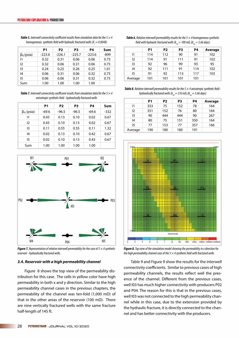
Similar to the anisotropic case in the previous chapter, the effective permeability in the x direction is tenfold the fracture permeability in the y direction. Table 7 and Fig-ure 6 show the results for the interwell connectivity coef-ficients. As expected, the results are good indications of the anisotropy with large coefficients for well pairs in the direction of high permeability. Table 8 and Figure 7 pres-ent the corresponding relative interwell permeabilities with the equivalent time of 5.66 days, and the reference permeability of 316 mD.

Figure 4. Representation of the interwell connectivity coefficients for the 5 × 4 homoge-neous system with hydraulically fractured wells.

Figure 5. Representation of the relative interwell permeability for the 5 × 4 homoge-neous reservoir with hydraulically fractured wells.

Figure 6. Representation of the connectivity coefficients for the case of 5 × 4 anisotropic reservoir - hydraulically fractured wells.

Figure 3. A zoom-in view of a LGR showing a high permeability strip representing a hydraulic fracture - 5 × 4 homogeneous system.

P03P02

P04

P01I01 I02

I04

I03

I05

P03P02

P04

P01I01 I02

I04

I03

I05

P03P02

P04

P01I01 I02

I04

I03

I05

P03P02

P04

P01I01 I02

I04

I03

I05

P03P02

P04

P01I01 I02

I04

I03

I05



3.4. Reservoir with a high permeability channel

Figure 8 shows the top view of the permeability dis-tribution for this case. The cells in yellow color have high permeability in both x and y direction. Similar to the high permeability channel cases in the previous chapters, the permeability of the channel was ten-fold (1,000 mD) of that in the other areas of the reservoir (100 mD). There are nine vertically fractured wells with the same fracture half-length of 145 ft.

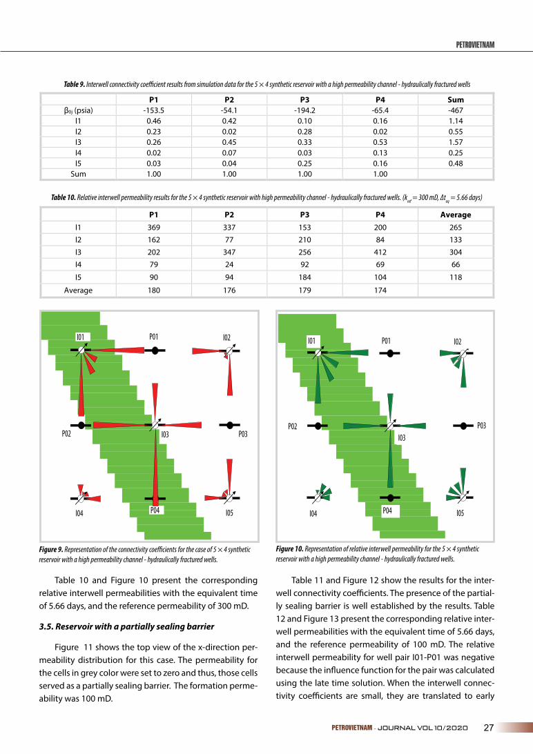
Table 9 and Figure 9 show the results for the interwell connectivity coefficients. Similar to previous cases of high permeability channels, the results reflect well the pres-ence of the channel. Different from the previous cases, well I03 has much higher connectivity with producers P02 and P04. The reason for this is that in the previous cases, well I03 was not connected to the high permeability chan-nel while in this case, due to the extension provided by the hydraulic fracture, it is directly connected to the chan-nel and has better connectivity with the producers.

Figure 8. Top view of the simulation model showing the permeability in x direction for the high permeability channel case of the 5 × 4 synthetic field with fractured wells.

Figure 7. Representation of relative interwell permeability for the case of 5 × 4 synthetic reservoir - hydraulically fractured wells.

Table 5. Interwell connectivity coefficient results from simulation data for the 5 × 4 homogeneous synthetic field with hydraulic fractured wells (As = 0.0048)

Table 6. Relative interwell permeability results for the 5 × 4 homogeneous synthetic field with hydraulic fractured wells (kref = 100 mD, Δteq = 5.66 days)

Table 7. Interwell connectivity coefficient results from simulation data for the 5 × 4 anisotropic synthetic field - hydraulically fractured wells

Table 8. Relative interwell permeability results for the 5 × 4 anisotropic synthetic field - hydraulically fractured wells (kref = 316 mD, Δteq = 5.66 days)

P1 P2 P3 P4 Sum β0j (psia) -223.6 -226.1 -225.7 -223.6 -899 I1 0.32 0.31 0.06 0.06 0.75 I2 0.32 0.06 0.31 0.06 0.75 I3 0.24 0.25 0.26 0.25 1.01 I4 0.06 0.31 0.06 0.32 0.75 I5 0.06 0.06 0.31 0.32 0.75 Sum 1.00 1.00 1.00 1.00

P1 P2 P3 P4 Average I1 114 112 90 91 102 I2 114 91 111 91 102 I3 92 96 99 93 95 I4 92 111 91 114 102 I5 91 92 113 117 103

Average 101 101 101 101

P1 P2 P3 P4 Sum β0j (psia) -69.6 -96.5 -96.5 -69.6 -332

I1 0.43 0.13 0.10 0.02 0.67

I2 0.43 0.10 0.13 0.02 0.67 I3 0.11 0.55 0.55 0.11 1.32

I4 0.02 0.13 0.10 0.42 0.67

I5 0.02 0.10 0.13 0.43 0.67

Sum 1.00 1.00 1.00 1.00


Average 190 180 180 191

P03P02

P04

P01I01 I02

I04

I03

I05


PETROVIETNAM

Table 10 and Figure 10 present the corresponding relative interwell permeabilities with the equivalent time of 5.66 days, and the reference permeability of 300 mD.

3.5. Reservoir with a partially sealing barrier

Figure 11 shows the top view of the x-direction per-meability distribution for this case. The permeability for the cells in grey color were set to zero and thus, those cells served as a partially sealing barrier. The formation perme-ability was 100 mD.

Table 11 and Figure 12 show the results for the inter-well connectivity coefficients. The presence of the partial-ly sealing barrier is well established by the results. Table 12 and Figure 13 present the corresponding relative inter-well permeabilities with the equivalent time of 5.66 days, and the reference permeability of 100 mD. The relative interwell permeability for well pair I01-P01 was negative because the influence function for the pair was calculated using the late time solution. When the interwell connec-tivity coefficients are small, they are translated to early

Figure 9. Representation of the connectivity coefficients for the case of 5 × 4 synthetic reservoir with a high permeability channel - hydraulically fractured wells.

Figure 10. Representation of relative interwell permeability for the 5 × 4 synthetic reservoir with a high permeability channel - hydraulically fractured wells.

P1 P2 P3 P4 Sum β0j (psia) -153.5 -54.1 -194.2 -65.4 -467

I1 0.46 0.42 0.10 0.16 1.14 I2 0.23 0.02 0.28 0.02 0.55 I3 0.26 0.45 0.33 0.53 1.57 I4 0.02 0.07 0.03 0.13 0.25 I5 0.03 0.04 0.25 0.16 0.48

Sum 1.00 1.00 1.00 1.00

Table 9. Interwell connectivity coefficient results from simulation data for the 5 × 4 synthetic reservoir with a high permeability channel - hydraulically fractured wells

P1 P2 P3 P4 Average I1 369 337 153 200 265 I2 162 77 210 84 133

I3 202 347 256 412 304 I4 79 24 92 69 66

I5 90 94 184 104 118

Average 180 176 179 174

Table 10. Relative interwell permeability results for the 5 × 4 synthetic reservoir with high permeability channel - hydraulically fractured wells. (kref = 300 mD, Δteq = 5.66 days)

P02

I01 I02

I04

I03

I05

P03

P04

P01

P02

I01 I02

I04

I03

I05

P03

P04

P01



time periods and thus the late time solution becomes in-accurate. Solutions that are good for both early time and late time should be used for better results.

3.6. Reservoir with a sealing barrier

Figure 14 shows the top view of the x-direction per-meability distribution with a sealing barrier case. The permeability of the cells in grey color was set to zero and thus, those cells served as a sealing barrier. As seen in the figure, the barrier completely divides the reservoir into

two compartments. Based on the change in average res-ervoir pressure calculated from each producer, this com-partmentalisation can be inferred.

Table 13 and Figure 15 show the results for the inter-well connectivity coefficients. Similar to previous cases, the results clearly reflect the presence of the sealing bar-rier. Some connectivity coefficients are very small and even negative. They indicate poor connectivity or no con-nectivity at all. Small connectivities were still observed for some pairs of wells on different sides of the sealing barrier.

Figure 11. Top view of the simulation model showing the permeability distribution in x direction for the case of 5 × 4 synthetic field with a partially sealing barrier - hydraulically fractured wells.

Figure 12. Representation of the connectivity coefficients for the case of 5 × 4 dual-porosity reservoir with a partially sealing barrier - hydraulically fractured wells.

P03P02

P04

P01I01 I02

I04

I03

I05

P1 P2 P3 P4 Sum β0j (psia) -440.1 -204.0 -306.9 -226.1 -1177

I1 0.01 0.34 0.01 0.06 0.42 I2 0.79 0.02 0.49 0.06 1.36 I3 0.06 0.25 0.08 0.22 0.61 I4 0.04 0.32 0.05 0.33 0.73 I5 0.11 0.07 0.37 0.33 0.87

Sum 1.00 1.00 1.00 1.00

P1 P2 P3 P4 Average I1 -40 127 68 90 62 I2 347 71 199 92 177 I3 23 95 29 83 58 I4 80 114 88 119 100 I5 115 95 141 125 119

Average 105 101 105 102

Table 11. Interwell connectivity coefficient results from simulation data for the 5 × 4 synthetic field with partially sealing barrier - hydraulically fractured wells

Table 12. Relative interwell permeability results for the 5 × 4 synthetic field with partially sealing barrier - hydraulically fractured wells (kref = 100 mD, Δteq = 5.66 days)


PETROVIETNAM

As explained before, these non-zero connectivity coeffi-cients are due to the noises in the data as the injection rates were generated randomly. This problem can be re-solved by increasing the number of data points. For this case, the interwell connectivity coefficients should be analysed with the average reservoir pressure change re-sults. If the pressure changes indicate reservoir compart-mentalisation, then the small interwell connectivity coef-ficients can be evaluated to decide whether the injectors and producers are on different side of the barrier.

Table 14 and Figure 16 present the corresponding relative interwell permeabilities with the equivalent time of 5.66 days, and the reference permeability of 100 mD. A cut-off coefficient of 0.06 was applied to eliminate the low connectivity coefficients. Thus, the relative interwell permeability corresponding to the coefficients lower than 0.06 were set to zeros. The resulting relative interwell per-meabilities show a clear presence of the sealing barrier.

Table 15 shows the results for the average reservoir pressure change for all producers in each case described

Figure 13. Representation of relative interwell permeability for the case of 5 × 4 dual-porosity reservoir with a partially sealing barrier - hydraulically fractured wells.

Figure 14. Top view of the simulation model showing the permeability in x direction for the case of 5 × 4 synthetic field with a sealing barrier - hydraulically fractured wells.

P02

I01 I02

I04

I03

I05

P03

P04

P01

Table 13. Interwell connectivity coefficient results from simulation data for the 5 × 4 synthetic field with a sealing barrier - hydraulically fractured wells

P1 P2 P3 P4 Sum β0j (psia) -336.6 -266.0 -225.4 -365.7 -1194

I1 0.00 0.35 0.00 0.10 0.45 I2 0.87 -0.01 0.60 -0.01 1.44 I3 0.05 0.27 0.05 0.35 0.73 I4 -0.02 0.36 -0.02 0.53 0.84 I5 0.07 0.04 0.35 0.05 0.51

Sum 0.97 1.01 0.97 1.02

Table 14. Relative interwell permeability results for the 5 × 4 synthetic field with a sealing barrier - hydraulically fractured wells (kref = 100 mD, Δteq = 5.66 days)

P1 P2 P3 P4 Average I1 0.00 131.5 0.00 112.5 61.01 I2 385.6 0.00 253.1 0.00 159.7 I3 0.00 101.7 0.00 132.6 58.6 I4 0.00 137.4 0.00 216.6 88.5 I5 98.2 0.00 132.6 0.00 57.7

Average 97 74 77 92



above. Similar to the results obtained from the previous systems, except for the case of sealing barrier, the changes in average reservoir pressure for all the cases are consis-tent and close to the pressure changes obtained from the simulation results. For the case with the presence of seal-ing barrier, the calculated pressure changes for wells P01 and P03 (about 181 psi) are different from those for wells P02 and P04 (about 390 psi) indicating two different pore volumes and thus, two different reservoir compartments.

4. Simulation results for horizontal wells

4.1. Model description for horizontal wells

Figure 17 shows the top view of the permeability distribution of the 5 × 4 homogeneous synthetic field with horizontal wells. All the wells were horizontal wells with their centres at the cell where the vertical wells were completed as described in the previous section (Table 3). Figure 18 shows the permeability distribution cross section cutting through three representative horizontal wells. Thus, all the wells were completed in the centre

Figure 15. Representation of the connectivity coefficients for the 5 × 4 synthetic field with a sealing barrier - hydraulically fractured wells.

Figure 16. Representation of relative interwell permeability for the 5 × 4 synthetic field with a sealing barrier - hydraulically fractured wells.

Figure 17. Top view of the simulation model showing the horizontal wells of the 5 × 4 homogeneous synthetic field.

P03P02

P04

P01I01 I02

I04

I03

I05

P02

I01 I02

I04

I03

I05

P03

P04

P01

Table 15. Average pressure change (ΔPave) after each time interval for different cases of 5 × 4 synthetic field - hydraulically fractured wells

Cases P1 P2 P3 P4 Homogeneous eservoir 285.93 285.93 285.74 285.74 Anisotropic reservoir 285.83 285.82 285.82 285.77 Channel 285.82 285.82 285.81 285.82 Partially sealing barrier 295.33 300.01 296.38 298.84 Sealing barrier 180.93 390.14 180.77 390.18


PETROVIETNAM

layer of the reservoir so that their distances to the top and bottom boundaries of the reservoir were equal. The for-mation permeability was set to 100 mD in the x, y and z directions. All wells are at the same length of 300 ft and completed along the x-direction. The wells were assumed to be infinite conductivity horizontal wells. Thus, the influ-ence functions were calculated using the pressure distri-bution equation (Equation 12) evaluated at the point xD = 0.732 and yD = ywD.

4.2. Homogeneous reservoir

Table 16 and Figure 19 show the results for the inter-well connectivity coefficients obtained from the simula-tion data for this case. Similar to the same cases in the previous section, the results are very close to the results obtained for the homogeneous reservoir with vertical wells. Small value of the asymmetry coefficient for this case (As = 0.00445) indicates good results for the interwell connectivity coefficients. Table 17 and Figure 20 present the corresponding relative interwell permeabilities with the equivalent time of 6.59 days, and the reference per-

Figure 19. Representation of the connectivity coefficients for the case of 5 × 4 homoge-neous reservoir with horizontal wells.

Figure 20. Representation of the relative interwell permeability for the case of 5 × 4 homogeneous reservoir with horizontal wells.

Figure 18. Cross sectional view showing three horizontal wells and their completions in the 5 × 4 homogeneous synthetic reservoir.

P03P02

P04

P01I01 I02

I04

I03

I05

P03P02

P04

P01I01 I02

I04

I03

I05

P1 P2 P3 P4 Sum β0j (psia) -291.9 -293.7 -294.0 -292.1 -1172

I1 0.29 0.30 0.08 0.09 0.76 I2 0.29 0.08 0.30 0.09 0.76 I3 0.24 0.24 0.25 0.23 0.96 I4 0.09 0.29 0.09 0.29 0.76 I5 0.09 0.09 0.29 0.30 0.76

Sum 1.00 1.00 1.00 1.00


Average 100 101 100 100

Table 16. Interwell connectivity coefficient results from simulation data for the 5 × 4 homogeneous synthetic field with horizontal wells (A = 0.00445)

Table 17. Relative interwell permeability results for the 5 × 4 homogeneous synthetic field with horizontal wells (kref = 100 mD, Δteq = 6.59 days)



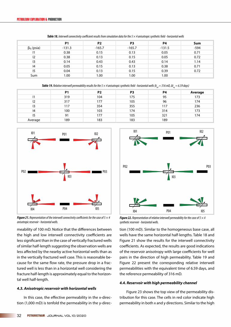
meability of 100 mD. Notice that the differences between the high and low interwell connectivity coefficients are less significant than in the case of vertically fractured wells of similar half-length suggesting the observation wells are less affected by the nearby active horizontal wells than as in the vertically fractured well case. This is reasonable be-cause for the same flow rate, the pressure drop in a frac-tured well is less than in a horizontal well considering the fracture half-length is approximately equal to the horizon-tal well half-length.

4.3. Anisotropic reservoir with horizontal wells

In this case, the effective permeability in the x-direc-tion (1,000 mD) is tenfold the permeability in the y-direc-

tion (100 mD). Similar to the homogeneous base case, all wells have the same horizontal half-lengths. Table 18 and Figure 21 show the results for the interwell connectivity coefficients. As expected, the results are good indications of the reservoir anisotropy with large coefficients for well pairs in the direction of high permeability. Table 19 and Figure 22 present the corresponding relative interwell permeabilities with the equivalent time of 6.59 days, and the reference permeability of 316 mD.

4.4. Reservoir with high permeability channel

Figure 23 shows the top view of the permeability dis-tribution for this case. The cells in red color indicate high permeability in both x and y directions. Similar to the high

P1 P2 P3 P4 Sum β0j (psia) -131.3 -165.7 -165.7 -131.5 -594

I1 0.38 0.15 0.13 0.05 0.71 I2 0.38 0.13 0.15 0.05 0.72 I3 0.14 0.43 0.43 0.14 1.14 I4 0.05 0.15 0.13 0.38 0.71 I5 0.04 0.13 0.15 0.39 0.72

Sum 1.00 1.00 1.00 1.00

Table 18. Interwell connectivity coefficient results from simulation data for the 5 × 4 anisotropic synthetic field - horizontal wells


Average 189 183 183 189

Table 19. Relative interwell permeability results for the 5 × 4 anisotropic synthetic field - horizontal wells (kref = 316 mD, Δteq = 6.59 days)

Figure 21. Representation of the interwell connectivity coefficients for the case of 5 × 4 anisotropic reservoir - horizontal wells.

Figure 22. Representation of relative interwell permeability for the case of 5 × 4 synthetic reservoir - horizontal wells.

P03P02

P04

P01I01 I02

I04

I03

I05

P03P02

P04

P01I01 I02

I04

I03

I05


PETROVIETNAM

permeability channel cases in the previous chapters, the permeability of the channel was ten-fold (1,000 mD) of that in the other areas of the reservoir (100 mD). There are nine horizontal wells with the same horizontal well half-length of 150 ft.

Table 20 and Figure 24 show the results for the inter-well connectivity coefficients. Similar to the fractured well case of a reservoir with high permeability channel, the re-sults reflect accurately the presence of the channel. Table 21 and Figure 25 present the corresponding relative inter-well permeabilities with the equivalent time of 6.59 days, and the reference permeability of 300 mD.

4.5. Reservoir with a partially sealing barrier

Figure 26 shows the top view of the x-direction per-meability distribution for this case. The cells in white color were inactive and thus, served as a partially sealing bar-rier. The formation permeability was 100 mD. Table 22 and Figure 26 show the results for the interwell connectivity coefficients. The presence of the partially sealing barrier is well established based on the results. Table 23 and Fig-ure 28 present the corresponding relative interwell per-meabilities with the equivalent time of 6.59 days, and the reference permeability of 100 mD. Similar to the same case for fractured wells, the relative interwell permeability

Figure 23. Top view of the simulation model showing the permeability in x-direction for the high permeability channel case of the 5 × 4 synthetic field - horizontal wells.

Figure 24. Representation of the connectivity coefficients for the high permeability channel case of the 5 × 4 synthetic field - horizontal wells.

P03P02

P04

P01I01 I02

I04

I03

I05

P1 P2 P3 P4 Sum β0j (psia) -197.5 -73.2 -241.7 -83.5 -596

I1 0.46 0.45 0.14 0.22 1.27 I2 0.20 0.03 0.25 0.04 0.51 I3 0.26 0.41 0.34 0.48 1.50 I4 0.03 0.07 0.05 0.12 0.27 I5 0.04 0.04 0.21 0.15 0.45

Sum 1.00 1.00 1.00 1.00

Table 20. Interwell connectivity coefficient results from simulation data for the high permeability channel case of the 5 × 4 synthetic field - horizontal wells

Table 21. Relative interwell permeability results for the high permeability channel case of the 5 × 4 synthetic field - horizontal wells (kref = 300 mD, Δteq = 6.59 days)


Average 180 177 178 175



for well pair I01-P01 was negative because the influence function for the pair was calculated using the late time solution. When the interwell connectivity coefficients are small, they are translated to early time-periods and, thus, the late time solution becomes inaccurate. Thus, the negative value was set to zero due to small connectivity coefficient.

4.6. Reservoir with a sealing barrier

Figure 29 shows the top view of the x-direction per-meability distribution for the sealing barrier case. The cells in white colour were inactive and thus, served as a seal-

ing barrier. As seen on the figure, the barrier completely divides the reservoir into two compartments. Based on the change in average reservoir pressure calculated from each producer, the compartmentalisation can be inferred.

Table 24 and Figure 30 show the results for the in-terwell connectivity coefficients. Similar to the previous cases, the results clearly reflect the presence of the seal-ing barrier. Some connectivity coefficients are very small and even negative. They indicate poor connectivity or no connectivity at all.

Table 25 and Figure 31 present the corresponding

Figure 25. Representation of relative interwell permeability for the high permeability channel case of the 5 × 4 synthetic field - horizontal wells.

Figure 26. Top view of the simulation model showing the permeability distribution in x direction for the 5 × 4 synthetic field with partially sealing barrier - horizontal wells.

P03P02

P04

P01I01 I02

I04

I03

I05

P1 P2 P3 P4 Sum β0j (psia) -540.6 -260.1 -391.4 -291.3 -1483

I1 0.01 0.34 0.02 0.09 0.46 I2 0.73 0.03 0.47 0.09 1.31 I3 0.07 0.24 0.10 0.22 0.63 I4 0.05 0.30 0.07 0.30 0.73 I5 0.13 0.09 0.34 0.31 0.87

Sum 1.00 1.00 1.00 1.00

P1 P2 P3 P4 Average I1 -32 130 64 97 65 I2 321 67 195 96 170 I3 30 93 38 85 62 I4 80 114 89 111 98 I5 119 98 130 115 116

Average 104 101 103 101

Table 22. Interwell connectivity coefficient results from simulation data for the 5 × 4 synthetic field with partially sealing barrier - horizontal wells

Table 23. Relative interwell permeability results for the 5 × 4 synthetic field with partially sealing barrier - horizontal wells (kref = 100 mD, Δteq = 6.59 days)


PETROVIETNAM

relative interwell permeabilities with the equivalent time of 6.59 days, and the reference permeability of 100 mD. A cut-off coefficient of 0.06 was applied to eliminate the low connectivity coefficients. Thus, the relative interwell permeability corresponding to the coefficients lower than 0.06 were set to zeros. The resulting relative interwell per-meabilities show a clear presence of the sealing barrier (Figure 31).

Table 26 shows the results for the average reservoir pressure change for all producers in each representative case described in this section. Similar to the previous sec-tion, the changes in average reservoir pressure for all the cases are about the same and close to the simulated pres-sure changes. For the case with the presence of a sealing barrier, the resulting pressure changes for wells P01 and

Figure 27. Representation of the connectivity coefficients for the case of 5 × 4 dual-porosity reservoir with a partially sealing barrier - horizontal wells.

Figure 29. Top view of the simulation model showing the permeability in x direction for the case of 5 × 4 synthetic field with a sealing barrier - horizontal wells.

Figure 28. Representation of relative interwell permeability for the case of 5 × 4 dual-porosity reservoir with a partially sealing barrier - horizontal wells.

Figure 30. Representation of the connectivity coefficients for the 5 × 4 synthetic field with a sealing barrier - horizontal wells.

P03P02

P04

P01I01 I02

I04

I03

I05

P03P02

P04

P01I01 I02

I04

I03

I05

P03P02

P04

P01I01 I02

I04

I03

I05



P03 (about 181 psi) are different from those for wells P02 and P04 (390 psi) indicating two different reservoir com-partments. Thus, the reservoir pressure change results are consistent.

5. Results for mixed wellbore conditions

5.1. Mixed case of fully penetrating vertical wells and fully penetrating hydraulic fractures

Figure 32 shows the top view of the permeability dis-

P1 P2 P3 P4 Sum β0j (psia) -336.6 -266.0 -225.4 -365.7 -1194

I1 0.00 0.35 0.00 0.10 0.45 I2 0.87 -0.01 0.60 -0.01 1.44 I3 0.05 0.27 0.05 0.35 0.73 I4 -0.02 0.36 -0.02 0.53 0.84 I5 0.07 0.04 0.35 0.05 0.51

Sum 0.97 1.01 0.97 1.02

Table 24. Interwell connectivity coefficient results from simulation data for the 5 × 4 synthetic field with a sealing barrier - horizontal wells


Average 96 77 79 93

Table 25. Relative interwell permeability results for the 5 × 4 synthetic field with a sealing barrier - horizontal wells (kref = 100 mD, Δteq = 6.59 days)

Figure 31. Representation of relative interwell permeability for the 5 × 4 synthetic field with a sealing barrier - horizontal wells.

Figure 32. Top view of the simulation model showing the x-direction permeability for the 5 × 4 homogeneous synthetic field - mixed hydraulically fractured and vertical wells.

P03P02

P04

P01I01 I02

I04

I03

I05

Cases P1 P2 P3 P4 Homogeneous reservoir 285.98 286.04 285.79 285.84 Anisotropic reservoir 285.93 285.92 285.92 285.79 Channel 285.90 285.94 285.82 285.91 Partially sealing barrier 294.99 300.45 296.10 298.96 Sealing barrier 180.93 390.14 180.77 390.18

Table 26. Average pressure change (ΔPave) after each time interval for different cases of 5 × 4 synthetic field - horizontal wells


PETROVIETNAM

tribution for this case. As shown on the figure, wells I01, P01, I03, P03 and I05 are hydraulically fractured wells and all the other wells are fully penetrating vertical wells. Table 27 and Figure 33 present the interwell connectivity coef-ficient results for this case. It is obvious that hydraulically fractured injectors have better connectivity with the pro-ducers than the vertical injectors.

Table 28 and Figure 34 show the corresponding rela-tive interwell permeability results for this reservoir. The relative permeabilities for the well pairs of vertical injec-tors are slightly lower than those of hydraulic fractures. However, the calculated relative interwell permeability

is in good agreement with the input permeability for the model of 100 mD.

Figure 35 shows the comparison of the interwell con-nectivity coefficients results obtained from simulation data and calculations using influence functions. The coef-ficients are in good agreement with R2 = 0.9875.

5.2. Mixed case of fully penetrating vertical wells and horizontal wells

Figure 36 shows the top view of the permeability dis-tribution for this case. As shown on the figure, wells I01, P01, I03, P03 and I05 are horizontal wells and all the other

Figure 33. Representation of the connectivity coefficients for the 5 × 4 homogeneous synthetic field - mixed hydraulically fractured and vertical wells.

Figure 34. Representation of relative interwell permeability for the 5 × 4 homogeneous synthetic field - mixed hydraulically fractured and vertical wells.

P03P02

P04

P01I01 I02

I04

I03

I05

P03P02

P04

P01I01 I02

I04

I03

I05

P1 P2 P3 P4 Sum β0j (psia) -281.1 -502.1 -282.1 -501.9 -1567

I1 0.37 0.36 0.10 0.11 0.94 I2 0.16 0.04 0.16 0.04 0.41 I3 0.32 0.33 0.34 0.33 1.32 I4 0.04 0.16 0.04 0.16 0.41 I5 0.11 0.11 0.35 0.36 0.93

Sum 1.00 1.00 1.00 1.00


Average 96 96 96 97

Table 27. Interwell connectivity coefficient results from simulation data for the 5 × 4 homogeneous synthetic field - mixed hydraulically fractured and vertical wells

Table 28. Relative interwell permeability results for the 5 × 4 homogeneous synthetic field - mixed hydraulically fractured and vertical wells (kref = 100 mD, Δteq = 7.33 days)



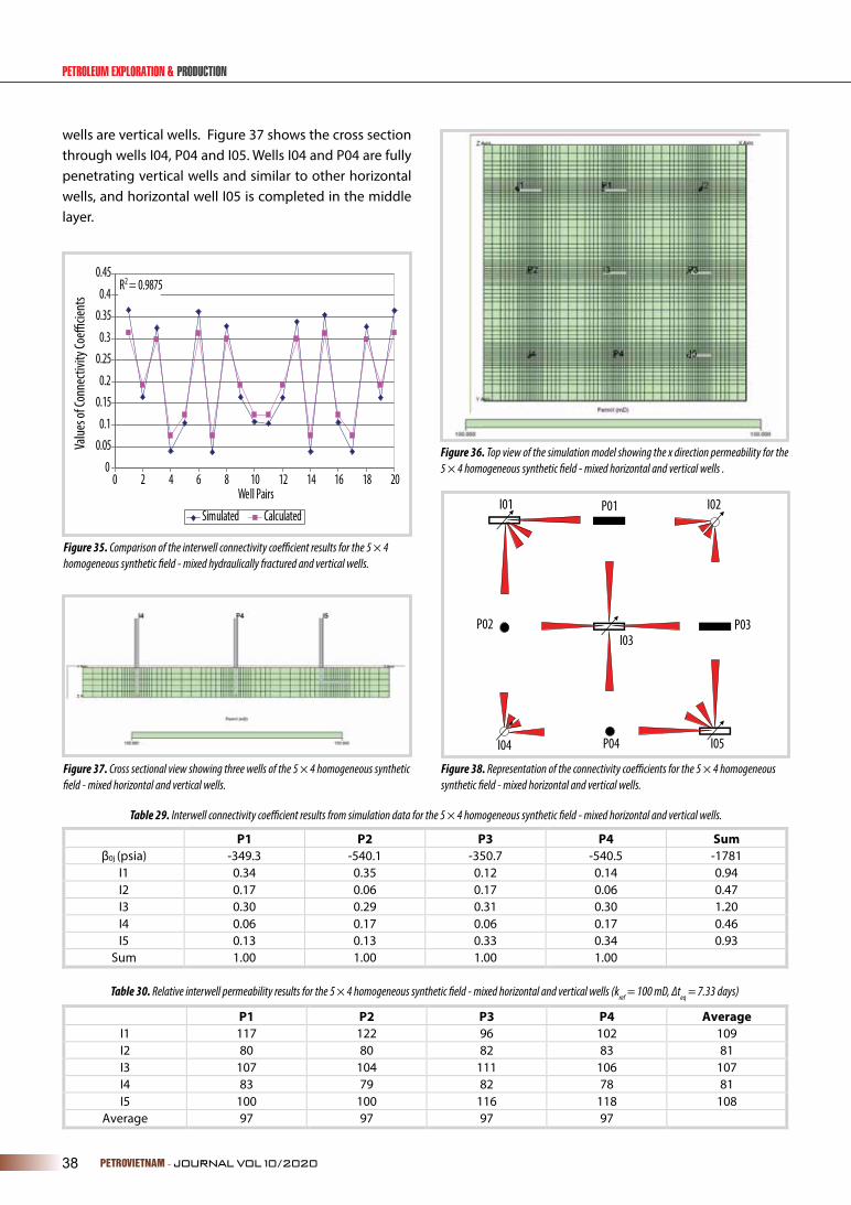
wells are vertical wells. Figure 37 shows the cross section through wells I04, P04 and I05. Wells I04 and P04 are fully penetrating vertical wells and similar to other horizontal wells, and horizontal well I05 is completed in the middle layer.

Figure 35. Comparison of the interwell connectivity coefficient results for the 5 × 4 homogeneous synthetic field - mixed hydraulically fractured and vertical wells.

Figure 36. Top view of the simulation model showing the x direction permeability for the 5 × 4 homogeneous synthetic field - mixed horizontal and vertical wells .

Figure 37. Cross sectional view showing three wells of the 5 × 4 homogeneous synthetic field - mixed horizontal and vertical wells.

Figure 38. Representation of the connectivity coefficients for the 5 × 4 homogeneous synthetic field - mixed horizontal and vertical wells.

0

0.050.1

0.150.2

0.250.3

0.350.4

0.45

0 2 4 6 8 10 12 14 16 18 20Well Pairs

Simulated Calculated

R2 = 0.9875

Value

s of C

onne

ctivit

y Coe

�cie

nts

P03P02

P04

P01I01 I02

I04

I03

I05

P1 P2 P3 P4 Sum β0j (psia) -349.3 -540.1 -350.7 -540.5 -1781

I1 0.34 0.35 0.12 0.14 0.94 I2 0.17 0.06 0.17 0.06 0.47 I3 0.30 0.29 0.31 0.30 1.20 I4 0.06 0.17 0.06 0.17 0.46 I5 0.13 0.13 0.33 0.34 0.93

Sum 1.00 1.00 1.00 1.00

Table 29. Interwell connectivity coefficient results from simulation data for the 5 × 4 homogeneous synthetic field - mixed horizontal and vertical wells.


Average 97 97 97 97

Table 30. Relative interwell permeability results for the 5 × 4 homogeneous synthetic field - mixed horizontal and vertical wells (kref = 100 mD, Δteq = 7.33 days)


PETROVIETNAM

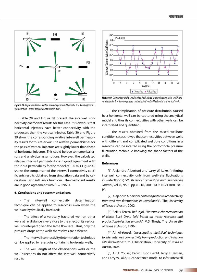
Table 29 and Figure 38 present the interwell con-nectivity coefficient results for this case. It is obvious that horizontal injectors have better connectivity with the producers than the vertical injector. Table 30 and Figure 39 show the corresponding relative interwell permeabil-ity results for this reservoir. The relative permeabilities for the pairs of vertical injectors are slightly lower than those of horizontal injectors. This could be due to numerical er-rors and analytical assumptions. However, the calculated relative interwell permeability is in good agreement with the input permeability for the model of 100 mD. Figure 40 shows the comparison of the interwell connectivity coef-ficients results obtained from simulation data and by cal-culation using influence functions. The coefficient results are in good agreement with R2 = 0.9681.

6. Conclusions and recommendations

- The interwell connectivity determination technique can be applied to reservoirs even when the wells are hydraulically fractured;

- The effect of a vertically fractured well on other wells at far distance is very close to the effect of its vertical well counterpart given the same flow rate. Thus, only the pressure drops at the wells themselves are different;

- The interwell connectivity determination technique can be applied to reservoirs containing horizontal wells;

- The well length at the observations wells or the well directions do not affect the interwell connectivity results;

- The complication of pressure distribution caused by a horizontal well can be captured using the analytical model and thus its connectivities with other wells can be interpreted and quantified.

- The results obtained from the mixed wellbore condition cases showed that connectivities between wells with different and complicated wellbore conditions in a reservoir can be inferred using the bottomhole pressure fluctuation technique knowing the shape factors of the wells.

References

[1] Alejandro Albertoni and Larry W. Lake, “Inferring interwell connectivity only from well-rate fluctuations in waterfloods”, SPE Reservoir Evaluation and Engineering Journal, Vol. 6, No. 1, pp. 6 - 16, 2003. DOI: 10.2118/83381-PA.

[2] Alejandro Albertoni, “Inferring interwell connectivity from well-rate fluctuations in waterfloods”, The University of Texas at Austin, 2002.

[3] Belkis Teresa Refunjol, “Reservoir characterization of North Buck Draw field based on tracer response and production/injection analysis”, M.S. Thesis, The University of Texas at Austin, 1996.

[4] Ali Al-Yousef, “Investigating statistical techniques to infer interwell connectivity from production and injection rate fluctuations”, PhD Dissertation. University of Texas at Austin, 2006.

[5] Ali A. Yousef, Pablo Hugo Gentil, Jerry L. Jensen, and Larry W.Lake, “A capacitance model to infer interwell

Figure 39. Representation of relative interwell permeability for the 5 × 4 homogeneous synthetic field - mixed horizontal and vertical wells.

Figure 40. Comparison of the simulated and calculated interwell connectivity coefficient results for the 5 × 4 homogeneous synthetic field - mixed horizontal and vertical wells.

P03P02

P04

P01I01 I02

I04

I03

I05

00.050.1

0.150.2

0.250.3

0.350.4

0.45

0 2 4 6 8 10 12 14 16 18 20Well Pairs

Simulated Calculated

R2 = 0.9681

Value

s of C

onne

ctivit

y Coe

�cie

nts



connectivity from production and injection rate fluctuations”, SPE Reservoir Evaluation & Engineering, Vol. 9, No. 6, pp. 630 - 646, 2006. DOI: 10.2118/95322-PA.

[6] Djebbar Tiab, "Inferring interwell connectivity from well bottom hole pressure fluctuations in waterfloods", SPE Production and Operations Symposium, Oklahoma, USA, 31 March - 3 April 2007. DOI: 10.2118/106881-MS.

[7] Djebbar Tiab and Dinh Viet Anh, “Inferring interwell connectivity from well bottom hole pressure fluctuations in waterfloods”, SPE Reservoir Evaluation & Engineering, Vol. 11, No. 5, pp. 874 - 881. DOI: 10.2118/106881-PA.

[8] Dinh Viet Anh and Djebbar Tiab, “Interpretation of interwell connectivity tests in a waterflood system”, SPE Annual Technical Conference and Exhibition, Denver, Colorado, USA, 21 - 24 September, 2008.

[9] Dinh Viet Anh, “Interwell connectivity tests in waterflood systems”, PhD Dissertation, University of Oklahoma, 2009.

[10] Taufan Marhaendrajana, “Modeling and analysis of flow behavior in single and multiwell bounded reservoirs”, PhD Dissertation, Texas A&M University, 1999.

[11] T. Marhaendrajana, N.J. Kaczorowski, and T.A. Blasingame, “Analysis and interpretation of well test

performance at Arun field, Indonesia”, SPE Annual Technical Conference and Exhibition, Houston, Texas, 3 - 6 October, 1999. DOI: 10.2118/56487-MS.

[12] D.N. Dietz, “Determination of average reservoir pressure from build-up survey”, JPT, Vol. 17, No. 8, pp. 955 - 959, 1965. DOI: 10.2118/1156-PA.

[13] E. Ozkan, “Performance of horizontal wells”, PhD Dissertation, University of Tulsa, 1988.

[14] Alain C. Gringarten, Henry J. Ramey Jr., and R. Raghavan, “Unsteady-state pressure distributions created by a well with a single infinite-conductivity vertical fracture”, Society of Petroleum Engineers Journal, Vol. 14, No. 4, pp. 347 - 360, 1974. DOI: 10.2118/4051-PA.

[15] Schlumberger, “ECLIPSE 100 black oil simulator” (version 2006.1), 2006.

[16] Heber Cinco-Ley and Fernando Samaniego-V, “Transient pressure analysis for fractured wells”, JPT, Vol. 33, No. 9, pp. 1749 - 1766, 1981. DOI: 10.2118/7490-PA.

[17] Djebbar Tiab, “Analysis of pressure derivative without type-curve matching: Vertically fractured wells in closed systems”, Journal of Petroleum Science and Engineering, Vol. 11, No. 4, pp. 323 - 333, 1994. DOI: 10.1016/0920-4105(94)90050-7.

inferring interwell connectivity in a reservoir from

Documents