individual motion of a charged particle in electric and magnetic fields
TRANSCRIPT

Chapter 2
Individual Motion of a ChargedParticle in Electric and MagneticFields
There are three distinct levels of modelling of the action of E and B fieldson the charged particles in a plasma. Starting with the simplest and movingto the most complicated, we have:
The single trajectory model
In this description, the fields E and B are given, imposed from the exte-rior: no account is taken of the fields created by the motion of the particles.Further, collisions are completely neglected, including Coulomb interactions:this model only describes the motion of an isolated particle.
The hydrodynamic model
In this case, the plasma consists either of two fluids (that of the electrons andthat of the ions), or of a single fluid (for instance, that of the electrons, the ionsremaining at rest and forming a continuous background, providing an effectiveviscosity to the electron motion). The motion of each fluid is characterisedlocally by an average velocity v whose value results from an integration ofthe velocity distribution of the particles contained in the volume elementconsidered (Sect. 3.3). The motion of the charged particles creates the fieldsE and B (for which the average local value is retained (macroscopic fields))which are included in a self-consistent manner in the equations of motion50.In addition, the model includes collisions, which modify the pre-determinedmotion defined by the superposition of the external and induced fields.
In order to establish self-consistency between the charged particle motionand the fields they produce, we need to consider first the velocity of the
50 The coupling of the E and B fields with the charged particles is said to be self-consistent
because the motion of the particles creating the fields E and B is itself influenced by thefields that it produces.
M. Moisan, J. Pelletier, Physics of Collisional Plasmas,DOI 10.1007/978-94-007-4558-2 2,© Springer Science+Business Media Dordrecht 2012
101

102 2 Motion of a charged particle in E and B fields
fluid elements. This is obtained from the equation of motion, in which theLorentz’ force (Sect. 2.1) is included, assuming values for the E and B fieldsfor the first iteration. Once v has been determined, we can calculate the totalcurrent density J from the component fluids involved (J =
∑α nαqαvα). We
can then complete the loop in two ways to obtain iterated values forE and B:
- from J , recover E from the electromagnetic relation:
J = σE , (2.1)
where σ is the electrical conductivity from the fluids involved, and from theknown value of E, calculate B by one or other of Maxwell’s curl equations:
∇ ∧E = −∂B
∂t, (2.2)
∇ ∧B = μ0ε0∂E
∂t+ μ0J , (2.3)
- from the density J , calculate the charge density ρ from the continuityequation (for example ∂ρ/∂t + ∇ · J = 0) and obtain E from Poisson’sequation:
∇ ·E = ρ/ε0 , (1.1)
then, determine B through (2.2) or (2.3).
Remark: Note that the conductivity σ, which relates J and E, plays a keyrole in obtaining field-particle self-consistence: we shall calculate the expres-sion for σ in the framework of various models.
The kinetic or microscopic model
This is the description with the highest resolution. It uses the individual ve-locity distributions of the particles: this allows us to include certain phenom-ena that escape the hydrodynamic model, such as, for example, the Landaudamping (resonance effect between a wave propagating in the plasma and par-ticles with velocities within a certain interval). This model includes the fieldsand collisions self consistently, this time on the microscopic scale (individualparticles), a more refined approach than that provided by the macroscopicvalues (average values over the velocity distribution of the particles).
The present chapter is devoted to the study of the individual motion ofa charged particle in given E and B fields. This model gives a first glimpseof the complex phenomena taking place at the heart of a plasma, with theassumption that there are no collisions in the body of the plasma or at thewalls. In the first place, we will examine the solution of the equation of

2.1 Equation of motion in E and B fields 103
motion through a series of particular cases, to finally determine the generalsolution51.
2.1 The general equation of motion of a charged particlein E and B fields and properties of that equation
Suppose qa is the charge of a particle of mass ma, moving with a velocity w =dr/dt and suppose E(r, t) and B(r, t) are the external fields: the particle issubject to the action of the Lorentz’ force that, in the non-relativistic case,takes the form52:
F ≡ qa [E(r, t) +w ∧B(r, t)] . (2.4)
This equation is the result of observation. It is valid if the particle is suffi-ciently small to be taken as a point (this therefore avoids the need to considerthe problem of repartition of charges in the particle volume).
2.1.1 The equation of motion
From (2.4), we can write:
mαd2r
dt2= qα
[
E(r, t) +dr
dt∧B(r, t)
]
. (2.5)
This equation leads to a second order differential equation for each axialcomponent of the coordinate system. For example, in Cartesian coordinates:
mαd2x
dt2= qα
[
Ex +
(
Bzdy
dt−By
dz
dt
)]
, (2.6)
mαd2y
dt2= qα
[
Ey +
(
Bxdz
dt−Bz
dx
dt
)]
, (2.7)
mαd2z
dt2= qα
[
Ez +
(
Bydx
dt−Bx
dy
dt
)]
. (2.8)
51 The principal reference for this section is Electrodynamics of Plasmas by Jancel andKahan, Chap. 4. See also Delcroix, Physique des plasmas, Vol. I, Sect. 12.3, Delcroix and
Bers, Physique des plasmas, Vol. I, Sect. 2.3, and Allis, Motions of Ions and Electrons [2].52 The relativistic equation is:
madw
dt= qa
(1− w2
c2
) 12[E(r, t) +w ∧B(r, t)− w2
c2(w ·E)
],
where c is the speed of light in vacuum.

104 2 Motion of a charged particle in E and B fields
2.1.2 The kinetic energy equation
Taking the scalar product of (2.5) with w = dr/dt, we obtain the kineticenergy equation:
mα
2
d
dt
∣∣∣∣dr
dt
∣∣∣∣
2
= qαE(r, t) · drdt
+ qα
(dr
dt∧B(r, t)
)
· drdt
, (2.9)
where the second term on the RHS vanishes, since (A ∧ B) · A = 0: theresulting equation is in scalar form and constitutes an invariant in any frameof reference. After integration of the equation over time t from t0 to t (inposition, from r0 to r), we have:
mα
2
[∣∣∣∣dr
dt
∣∣∣∣
2
r
−∣∣∣∣dr
dt
∣∣∣∣
2
r0
]
= qα
t∫
t0
E · dr , (2.10)
where the RHS of the equation represents the work done on the particle bythe electric field. From this, we can draw the following important conclusions:
1. The magnetic field does “no work” because the force it exerts on the par-ticle is perpendicular to its velocity53. It follows that the magnitude of thevelocity of a charged particle is not affected by the presence of a magneticfield. However, the magnitudes of the velocity components perpendicularto B can vary, as we will show for the cyclotron motion (Sect. 2.2.2).Supposing that B is directed along Ox, this implies that:
w2⊥ = w2
y0 + w2z0 = w2
y(t) + w2z(t) , (2.11)
where the subscript 0 denotes the velocity at t = 0: in other words, a mag-netic field can only change the direction of the velocity, not its magnitude.However, the application of a magnetic field to a plasma makes it possi-ble, among other things, to conserve the energy of the system by reducingthe diffusion losses of the charged particles to the walls, as we shall see(Sect. 3.8).
2. Only the electric field can “heat” the charged particles, i.e., give themenergy.
2.2 Analysis of particular cases of E and B
We will successively treat the following cases: only an electric field actingon the particle (Sect. 2.2.1); the particle is subjected to a constant, uniform
53 Heating by magnetic pumping, where B varies periodically, can be considered as result-ing from the action of the E field through the Maxwell equation ∇∧E = −∂B/∂t.

2.2 Analysis of particular cases of E and B 105
magnetic field, with or without an electric field E (Sect. 2.2.2); and finally,the most complex situation, the particle moves in a magnetic field that is(slightly) non uniform or (slowly) varying in time (Sect. 2.2.3). We will seethat the different solutions obtained for the particular cases can be includedin a general equation describing the particle motion in such E and B fields.
2.2.1 Electric field only (B = 0)
From (2.6), (2.7) and (2.8), we obtain:
d2x
dt2=
qama
Ex(r, t) ,d2y
dt2=
qama
Ey(r, t) ,d2z
dt2=
qama
Ez(r, t) . (2.12)
We can now treat the following cases.
Constant and uniform electric field E
By direct integration of (2.12) in vectorial form, we deduce:
w =qαmα
Et+w0 , (2.13)
r =qαmα
Et2
2+w0t+ r0 , (2.14)
which describe uniformly accelerated motion.
Remarks:
1. From (2.13), one can see that the component of motion along a directionperpendicular to E is not affected by the presence of this field; this can beshown by decomposing w in directions parallel and perpendicular to E.The situation is completely different with B, because the correspondingforce acts perpendicularly to B (and to w) (2.4).
2. Since the field E selectively accelerates the component of velocity parallelto it, we could say that it tends, if not to confine, at least to orient theparticle in this direction.
3. From (2.13) and (2.14), we can conclude that the velocity, as well as thedistance travelled by an ion of mass mi under the effect of a field E duringa given time is me/mi times smaller than that of an electron of mass me
in the same field, which justifies the commonly used assumption that theion is at rest with respect to the electron.

106 2 Motion of a charged particle in E and B fields
Conservative field E(r, t)
Since the electric field is conservative, we can write:
E = −∇φ(r, t) , (2.15)
where φ is the potential acting on the particle. The vectorial equation ofmotion:
mαd2r
dt2= −qα∇φ , (2.16)
scalar multiplied by dr/dt shows, after integration over time t, that the vari-ation of kinetic energy is equal to the (negative) variation of the potentialenergy, such that the total energy is, of course, conserved:
mα
2
[∣∣∣∣dr
dt
∣∣∣∣
2
r
−∣∣∣∣dr
dt
∣∣∣∣
2
r0
]
= −qα[φ(r, t)− φ(r0, t0)] . (2.17)
Equation (2.17) is a variant of (2.10).
Application to the case where φ is time independent
The motion of an electron in an electrostatic potential is similar to the prop-agation of a luminous wave in a medium of refractive index nr, as shownbelow.
Consider the case of two media where φ, moreover, does not depend on r,thus E is zero (2.15). The crossing of a discontinuity in potential (φ1 �= φ2,Fig. 2.1) determines the existence of a field E (at the interface only) and, asa result, the particle experiences an instantaneous acceleration (or decelera-tion), the velocity thus changing from w1 to w2.
However, the components of the velocities parallel to the interface betweenthe two media remain the same from one side to the other, because the electricfieldE is perpendicular to this interface (Remark 1 above) from which, notingp = mew:
|p1| sin θ1 = |p2| sin θ2 , (2.18)
which, when written in the form:
|p1||p2|
=sin θ2sin θ1
, (2.19)
appears as the well known geometrical optics law of Descartes, if θ1 andθ2 are considered as the angle of incidence and refraction respectively, andwhere the momentum pi of the particle is proportional to the index of themedium54.
54 Doing this, one finds that nr = A√E − qαφ, where A is a constant and E the total
energy of the particle.

2.2 Analysis of particular cases of E and B 107
Fig. 2.1 Description of the
refraction path in opticalelectronics.
The field E is uniform, but oscillates periodicallyas a function of time
This case corresponds to that in which the charged particles are present eitherin a plasma created by a high frequency field (HF), or in a plasma producedby other means (for example, a continuous current discharge) onto which asignificant HF field has been superimposed.
The equation of motion is, in this case:
d2r
dt2=
qαmα
E0eiωt (2.20)
and, after successive integrations from t = 0 to t, and supposing that theinitial velocity of the particle is w0 (taking w0 �= 0, to remain completelygeneral), we obtain:
w =dr
dt=
1
iω
[qαE0
mαeiωt − qαE0
mα
]
+w0 , (2.21)
or:
w =qαE0
imαωeiωt +
(
w0 −qαE0
iωmα
)
, (2.22)
and:
r = − qαE0
mαω2eiωt +
(
w0 −qαE0
iωmα
)
t+ rc , (2.23)
where rc is a constant of integration, the initial position of the particle being
r0 = − qαE0
mαω2+ rc . (2.24)
Examination of the relative phases of E, w and r
We consider a charged particle (taken to be a positive ion), with zero initialvelocity, in an electric field E0 cosωt of period T , and examine the detailed

108 2 Motion of a charged particle in E and B fields
behaviour of its velocity and trajectory55 as a function of time, with the aidof Fig. 2.2. To simplify this presentation, we ignore the non-periodic term invelocity in (2.22).
Fig. 2.2 Velocity and trajectory of a positive ion (full curve) and of an electron (dotted)
in an alternating electric field of period T .
1. Velocity: the velocity of the charged particle is in phase with the field E.From t = 0 to t = T /4, the positive ion is accelerated in the positivedirection of the field: its velocity increases during the entire quarter periodand reaches its maximum value at t = T /4, when the electric field passesthrough zero.Between t = T /4 and T /2, the field E is in the opposite direction to thevelocity of the positive ion, so it can only be retarded. The velocity passesthrough zero at the same time as the electric field reaches its maximum,the situation being symmetric to t = 0: in order to return to zero velocity,a field of the same amplitude but in the opposite direction is required.Between t = T /2 and 3T /4, by symmetry, the velocity of the particlereaches its maximum opposite to its initial direction at the same time as
55 By convention, the electric field existing between a positive charge and a negative charge
is directed towards the negative charge. As a result, a positive ion is accelerated in thedirection of the field (see Fig. 2.2).

2.2 Analysis of particular cases of E and B 109
the electric field passes through zero, just before changing sign, and soon. The velocity of the ion is then π/2 behind the phase of the field E.This de-phasing with respect to the field E, as we shall see, is such thatthe transfer of energy from the field to the charged particle is zero over acomplete period.
2. Trajectory: in the case of a positive ion, the phase of the trajectory lagsby π behind that of the electric field (in opposite phase), while an electronis in phase with the field. The amplitude of motion of a charged particlein a HF field E is referred to as the extension of the periodic motion anddenoted by xE .For a positive ion (initial position xE(0) in Fig. 2.2), since the initialvelocity is assumed to be zero, the direction of motion, according to ourconvention, is in the direction of the field and only changes direction whenthe velocity wE passes through zero (at t = T /2): at this time, the fieldhas its maximum in the opposite direction: there is clearly a lag in phaseof π in the motion of the ion in the field.In contrast, the spatial oscillation of the electron motion is in phase withthe HF field (following the convention of the direction of the field that wehave adopted).
Transfer of energy from an oscillating electric field Eto a charged particle
The kinetic energy resulting from the work done by an electric field E on thecharge, in the time interval t0 to t can be written (see (2.10)):
W ≡ mα
2w2
∣∣∣r
r0= qα
r∫
r0
E · dr = qα
t∫
t0
E ·wdt , (2.25)
and, following (2.22):
W = �
⎡
⎣qα
t∫
t0
E0eiωt ·
(qαE0
mαiωeiωt +w0 −
qαE20
iωmα
)
dt
⎤
⎦ ,
= �
⎡
⎣ q2αE20
imαω
t∫
t0
ei2ωtdt+
(
qαE0 ·w0 −q2αE
20
imαω
) t∫
t0
eiωtdt
⎤
⎦ ,
= �[
− q2αE20
2mαω2ei2ωt
∣∣∣∣
t
t0
+
(qαE0 ·w0
iω+
q2αE20
mαω2
)
eiωt
∣∣∣∣
t
t0
]
,
= − q2αE20
2mαω2cos 2ωt
∣∣∣∣
t
t0
+q2αE
20
mαω2cosωt
∣∣∣∣
t
t0
+qαE0 ·w0
ωsinωt
∣∣∣∣
t
t0
, (2.26)

110 2 Motion of a charged particle in E and B fields
where �(A) denotes the real part of a complex quantity A. In the scalarproduct under the integral, w reduces to wE (2.22), the component of thevelocity parallel to E (there is no work done in the direction perpendicularto E).
The value of the integral (2.26) over a period T = 2π/ω, i.e. between thetimes t0 and t0 + 2π/ω, is zero. The total kinetic energy acquired during aperiod is actually zero, because during the first half-period the work is donein one direction and in the opposite direction during the second half-period.
However, if the oscillatory motion of the particle is interrupted by a colli-sion before the repetition of a complete period starting from t0, when the fieldhas been applied, the integral (2.26) is non-zero and the corresponding energytaken from the field will be acquired by the particle56. In order to demon-strate this, we must leave the very simplified model of individual trajectories(collisionless plasma model) for a moment and consider the hydrodynamicmodel including collisions.
Transfer of energy from an oscillating field E to electrons viacollisions: power absorbed by the electrons and plasmapermittivity (a digression from individual trajectories)
Consider an electron fluid, coupled to ions and neutrals via collisions. As-suming that the thermal motion of electrons is negligible compared to theirmotion resulting from the field E (vth � vE , cold plasma approximation), thecorresponding hydrodynamic equation for momentum transport (Sect. 3.7)can then be written:
medv
dt= −eE0e
iωt −meνv , (2.27)
where v is the (macroscopic) velocity of electrons and ν the average electron-neutral momentum transfer collision frequency. The physical meaning of thisequation has already been discussed (1.147).
In fact, we are not very far from the context of individual trajectories inthe sense that we can consider that (2.27) describes the motion of a singleparticle in a medium where it is subject to a friction force.
In the cold plasma approximation, the electron velocity is purely periodic,such that:
v = v0eiωt , (2.28)
and, substituting v in (2.27), we obtain:
56 The particle “acquires” this energy at the moment of collision, this energy being totallyor partially shared with the particle with which it interacts. Recall that in the case of an
electron-neutral collision, the electron only partially transfers its energy; more exactly, afraction of the order of me/M of that energy (Sect. 1.7.2).

2.2 Analysis of particular cases of E and B 111
v = − eE(t)
me(ν + iω), (2.29)
which determines v0.Since dr/dt ≡ v, again neglecting thermal motion, we have:
r =v
iω, (2.30)
that is:
r =eE(t)
meω(ω − iν). (2.31)
- Average HF power absorbed per electronThe work per unit time and per electron in the field E can be written:
− eE · v , (2.32)
which thus represents the instantaneous power taken from the field. Theaverage value of the product of two complex variables A and B over aperiod, each varying sinusoidally with the same frequency, is �(AB∗)/2(B∗ is the complex conjugate of B). The power taken from the field overa period, or the average power, per electron, is then:
θa ≡ �(−eE · v∗
2
)
= �[e2E2
0
2me
1
(ν − iω)
]
=e2
me
ν
ν2 + ω2E2 , (2.33)
where√E2 = E0/
√2 is the mean squared value of the electric field.
If ν/ω � 1 (HF discharge approximation), we have (2.33):
θa ≈ e2
me
ν
ω2E2 , (2.34)
and we can verify that, for ν = 0, the transfer of energy from the field Eis zero, θa = 0, conforming to the result we have already obtained abovein the case of individual trajectories.In the opposite case of ν/ω 1 (low-frequency discharge approximation),we obtain:
θa ≈ e2
me
E2
ν. (2.35)
Expressions (2.34) and (2.35) are essential to the understanding of HFplasmas (Sect. 4.2).
- Electrical conductivity and permittivity in the presence of collisionsThe motion of charged particles in the field E creates a current, called theconduction current. For an electron density ne, the current density can bewritten:
J = −neev (2.36)

112 2 Motion of a charged particle in E and B fields
and in complex notation, following (2.29):
J =nee
2
me(ν + iω)E(t) . (2.37)
Since from electromagnetism:
J = σE , (2.38)
where σ is the (scalar) electrical conductivity of electrons, we find byidentification from (2.37) and (2.38):
σ =nee
2
me(ν + iω). (2.39)
Note that in the case where there are no collisions (ν = 0), σ is purelyimaginary and the plasma then behaves as a perfect dielectric.The permittivity εp of the plasma relative to vacuum in a field E0e
iωt isrelated to the conductivity σ (demonstrated in Remark 2 below):
εp = 1 +σ
iωε0, (2.40)
where ε0 is the permittivity of vacuum. Substituting σ from (2.39), wefind:
εp = 1−ω2pe
ω(ω − iν), (2.41)
which, in the absence of collisions, reduces to:
εp = 1−ω2pe
ω2, (2.42)
an expression which shows that the exact case where ω = ωpe representsa singular value for the propagation of a wave, since εp = 0.
Remarks:
1. Note that the value of θa (2.33) is inversely proportional to the mass of theparticles, which means that we can usually neglect the power transferredto the ions in assessing the HF-particle power balance. We can also verifythat for constant ω, θa passes through a maximum when ν = ω57; this isthe case in which the transfer of energy is the most efficient.
2. The use of the conductivity σ in the preceding pages corresponds to therepresentation of charges in vacuum, as distinct from the dielectric descrip-tion expressed by εp where, from the beginning, we prefer to consider the
57 Recall that the collision frequency ν depends on the average energy of the electrons(and on the energy distribution function) and gas pressure (Sect. 1.7.8).

2.2 Analysis of particular cases of E and B 113
displacement current rather than the conduction current to describe themotion of charged particles in a HF field.
In effect, in the case of a purely dielectric description of the plasma, (2.3) canbe expressed in the form:
∇ ∧B = μ0∂D
∂t≡ μ0ε0εp
∂E
∂t. (2.43)
Assuming a periodic variation eiωt in the electromagnetic field with angularfrequency ω, we obtain the terms on the RHS of (2.3) and (2.43) respectively:
μ0ε0∂E
∂t+ μ0J = μ0ε0iωE0e
iωt + μ0σE0eiωt , (2.44)
μ0ε0εp∂E
∂t= μ0ε0εpiωE0e
iωt , (2.45)
which, by identification, leads to:
iωε0εp = iωε0 + σ , (2.46)
from which we obtain the complex relative permittivity of the plasma givenby (2.40).
2.2.2 Uniform static magnetic field
MAGNETIC FIELD ONLY (E = 0)
The study of this simple case will allow us to introduce the concepts ofcyclotron gyration and helical motion. Cyclotron motion of particles producesa magnetic field B′, in the opposite direction to the externally applied fieldB, giving the plasma a diamagnetic character.
We will use Cartesian coordinates, such that Ox is oriented in the di-rection of B. From the general equations of motion (2.6) and (2.8), settingE = (0, 0, 0) and B = (B, 0, 0), we obtain:
d2x
dt2= 0 , (2.47)
d2y
dt2=
qαB
mα
dz
dt, (2.48)
d2z
dt2= −qαB
mα
dy
dt. (2.49)

114 2 Motion of a charged particle in E and B fields
These equations can be rewritten by introducing the cyclotron (angular)frequency :
ωcα = −qαB
mα, (2.50)
the sign convention being such that ωcα is positive for electrons58.Ignoring the subscript α for simplicity, (2.47) to (2.49) take the form:
x = 0 , (2.51)
y = −ωcz , (2.52)
z = ωcy . (2.53)
We will solve these equations, using the initial conditions (t = 0): x =y = z = 0 (the particle is initially at the origin of the coordinate system),x = wx0 = w‖0, y = wy0 and z = wz0: for complete generality, the compo-nents of the initial velocity parallel and perpendicular to B are non zero.Integrating (2.53), we obtain:
z = ωcy + C1 = ωcy + wz0 , (2.54)
where the constant of integration C1, in view of our initial conditions, is equalto wz0. Introducing this value of z into (2.52) for y;
y = −ω2cy − ωcwz0 . (2.55)
This equation can be rearranged such that the LHS is homogeneous in y:
y + ω2cy = −ωcwz0 , (2.56)
which has the form of a “forced” harmonic oscillator. The solution to thisequation is given by the sum of the general solution without the RHS, and aparticular solution of the differential equation including the RHS, thus:
y = A1 cosωct+A2 sinωct−wz0
ωc. (2.57)
We will now determine the constants A1 and A2 in (2.57):
y(t = 0) ≡ A1 −wz0
ωc= 0 from which A1 =
wz0
ωc, (2.58)
y(t = 0) ≡ wy0 = A2ωc from which A2 =wy0
ωc. (2.59)
We now need to calculate z(t): from (2.54) with (2.57)–(2.59),
58 Some authors prefer to write ωcα = |qα|B/mα, but it is still necessary to define the
direction in which the respective positively and negatively charged particles rotate arounda line of force of the field B.

2.2 Analysis of particular cases of E and B 115
z = ωc
[wz0
ωccosωct+
wy0
ωcsinωct−
wz0
ωc
]
+ wz0 , (2.60)
and, after integrating over t:
z =wz0
ωcsinωct−
wy0
ωccosωct+ C2 , (2.61)
and since z(t = 0) = 0, we find C2 = wy0/ωc.The three equations describing the orbit of a charged particle can finally bewritten:
x = wx0t = w‖0t , (2.62)
y =wz0
ωccosωct+
wy0
ωcsinωct−
wz0
ωc, (2.63)
z =wz0
ωcsinωct−
wy0
ωccosωct+
wy0
ωc. (2.64)
In the yOz plane, the particle motion describes a circle59, for which the centreis fixed by the constants of integration, in this case Y, Z = −wz0/ωc,−wy0/ωc.To demonstrate this, we will write the equation of the corresponding circulartrajectory:
(y − Y )2 + (z − Z)2 ≡(
y +wz0
ωc
)2
+
(
z − wy0
ωc
)2
=w2
z0
ω2c
cos2 ωct+w2
y0
ω2c
sin2 ωct+2wz0wy0
ω2c
cosωct sinωct
+w2
z0
ω2c
sin2 ωct+w2
y0
ω2c
cos2 ωct−2wz0wy0
ω2c
cosωct sinωct
=w2
z0 + w2y0
ω2c
≡ w2⊥0
ω2c
= r2B , (2.65)
from which we can define a radius whose value is:
rB =w⊥0
ωc=
me
eBw⊥0 . (2.66)
In summary, in the plane perpendicular to B, we observe a periodic cir-cular motion with an angular frequency ωc, the cyclotron frequency60, whose
59 The relations (2.63) and (2.64) which describe a periodic motion have the same ampli-tude and the same frequency, with a difference of phase π/2. In the framework of Lissajous
curves, this gives rise to a circle. Note that, in English, the distinction between frequencyand angular frequency is often ignored.60 Equivalently, the gyro-frequency of particles α (α = e, i).

116 2 Motion of a charged particle in E and B fields
radius rB is called the Larmor radius61, w⊥0 being the initial speed of theparticle in the yOz plane. To determine the direction of rotation of particlesof mass mα and of charge qα, we ignore the constant, initial velocity of theparticle in the yOz plane. For the electron, since by convention ωce > 0, wesee from (2.63) and (2.64) that for ωct = 0, y = wz0/ωc and z = −wy0/ωc,while for ωct = π/2 (t = Tc/4, where Tc is the cyclotron period), y = wy0/ωc
and z = wz0/ωc. It follows that, for a field B away from the reader, thegyration of the electron is in the clockwise direction (towards the right), as isshown in Fig. 2.3a, while the positive ion rotates in the anti-clockwise direc-tion (towards the left). In the direction parallel to B, the velocity is constant,equal to w‖0, and the motion is uniform, since this velocity is not modifiedby B. The combination of the cyclotron motion and uniform motion givesrise to a trajectory in the form of a helix (Fig. 2.3b), which rotates aroundthe magnetic field line (referred to as the guiding centre).
Fig. 2.3 a Cyclotron motion of an electron in the plane perpendicular to B, the fielddirected along the Ox axis, away from the reader. The points on the circle show the
position of the electron at t = 0 and t = Tc/4. b Helical motion of the electron along theB field.
Interesting particular cases:
- If w‖0 = 0, the helical trajectory degenerates into a circular orbit. Theradius of the orbit is then dependent on the total velocity w0 of the particle,and rB = w0me/eB.
- If w⊥0 = 0, the trajectory is rectilinear and parallel to B.
Remarks:
1. The decrease in the diameter of the helix with increasing B results in aconfinement of charged particles in the direction perpendicular to B. Infact, as B tends to infinity, rB → 0, such that transverse motion is not
61 Equivalently, the cyclotron radius or radius of gyration.

2.2 Analysis of particular cases of E and B 117
possible: we will see in Sect. 3.8 that this effect reduces the particle diffu-sion perpendicular to B, towards the walls.
2. A uniform fieldB cannot affect w‖ so w‖(t) = w‖0 where the subscript zerocorresponds to the time t = 0: this is a property of the Lorentz force in thecase E = 0. If E = 0, from conservation of kinetic energy: w2
⊥(t)+w2‖(t) ≡
w2(t) = w20. Since we have just seen that w‖ = w‖0, then w2
⊥ = w2⊥0 and,
thus w2⊥(t) ≡ w2
y(t)+w2z(t) = w2
⊥0. Thus, in a field B, the components wy
and wz can vary, as was mentioned in Sect. 2.1 (Remark 1).3. The pitch of the helix is obtained by calculating the axial distance travelled
during one revolution. If this pitch is ph, and Tc is the cyclotron period,then ph = w‖0Tc = w‖0/fc = 2πw‖0/ωc, and we obtain:
ph = 2π
(w‖0
w⊥0
)
rB . (2.67)
4. A useful way to represent the helical motion is:
w = w‖0 + ωc ∧ rB , (2.68)
where w‖0 describes the motion of the guiding centre and the second term,the circular cyclotron motion of the particle; the vector ωc is directed alongB and defines the axis of rotation and its direction; the vector rB , the orbitradius, has its origin at the guiding centre.
5. Since the Larmor radius is proportional to the mass of the particles, (see(2.66)), it follows that for ions of massmi, rBi = rBemi/me, i.e. rBi rBe.
6. The cyclotron frequency (2.50) or gyration frequency does not dependon the velocity of the particles, but only on their mass and charge. Thisproperty allows energy to be given uniquely to particles of a given mass andcharge by means of an electric field oscillating at ω = ωcα, independentlyof their velocity distribution: we can therefore obtain a form of selectiveheating by means of cyclotron resonance, which will be treated in detaillater (2.146).
7. A usefull numerical relation to calculate the cyclotron frequency for elec-trons is:
fce(Hz) = 2.799× 10¹⁰B (tesla) . (2.69)
Thus for B = 0.1T (103 gauss), fce = 2.8GHz. The corresponding fre-quency for ions of mass mi is mi/me times smaller.
8. The diamagnetic field created by the circulating cyclotron current is givenby the Biot-Savart Law (Lorrain et al):
B′ =μ0
4π
∫
V
J ∧ r
r3dV . (2.70)
In this expression, r points from the source (charge) towards the guidingcentre axis (Fig. 2.4). Note that B and B′ are calculated at the same r

118 2 Motion of a charged particle in E and B fields
position for comparison purposes. The diamagnetic field B′ points in thesame direction for electrons and ions: particles of opposite charge revolvein opposite directions around B, such that their respective currents rotatein the same direction, as is shown in Fig. 2.4. The vectorial product J ∧r from (2.70) indicates that B′ is in the opposite direction to the fieldB responsible for the cyclotron motion (this cannot be otherwise!). Themagnetic field in the plasma is given by the vectorial sum of B and B′
(see exercise 2.2).
Fig. 2.4 Determining the orientation of the diamagnetic field B′ created by the cy-
clotron motion in a field B imposed into the page: B′ comes out of the page towardsthe reader.
STATIC UNIFORM ELECTRIC AND MAGNETIC FIELDS
In this section, we will show that the effect of uniform, constant fields E andB leads to a motion, called the electric field drift (also known as the E ∧Bdrift), of ions and electrons in the plasma, perpendicular to both E and B.After this, we will derive an equation that incorporates all the fundamentalmotions studied to date. As a further application, we will calculate the electricconductivity, for the same E and B fields, and show that it is a tensor.
In the first case, the superposition of electric and magnetic fields modifiesthe magnitude of the velocity, such that the part of the Lorentz force tiedto the magnetic field, qαw ∧ B, is continuously varying. It is noteworthythat, since the two fields are uniform and constant in time, the orbits can becalculated analytically and are easily represented graphically.

2.2 Analysis of particular cases of E and B 119
The case where E and B are arbitrarily oriented (with w0 = 0)
The Cartesian frame is once again constructed such that B is directed alongthe Ox axis. Since the orientation of E in this frame is independent of B, theE field has a component along each of the axes. We suppose that the chargedparticle, at t = 0, is situated at the origin of the frame x = y = z = 0, and,in contrast to the previous case (B only), at rest x = y = z = 0. This lastcondition implies that w⊥0 = 0, removing the contribution of the cyclotronmotion to the particle trajectory entirely, allowing us to examine the effect ofthe electric field drift alone (the case w⊥0 �= 0 is treated further in the text,for E perpendicular and parallel to B.)
1. The equations of motionFrom (2.6)–(2.8), we obtain:
x =qαmα
Ex , (2.71)
y =qαmα
Ey − ωcz , (2.72)
z =qαmα
Ez + ωcy . (2.73)
2. Calculation of the trajectoriesThe equations of motion are integrated analogously to the previous case.Calculation of y: Integration of (2.73) gives:
z =qαmα
Ezt+ ωcy . (2.74)
Substituting z in (2.72):
y =qαmα
Ey − ωc
[qαmα
Ezt+ ωcy
]
. (2.75)
This equation can be rearranged such that the LHS is homogeneous:
y + ω2cy = −ωcqα
mαEzt+
qαmα
Ey , (2.76)
for which the solution is:
y = A1 cosωct+A2 sinωct−qα
mαωcEzt+
qαmαω2
c
Ey . (2.77)
The constants A1 and A2 are fixed by the initial conditions.Since y(t = 0) = 0, (2.77) yields:
A1 +qα
mαω2c
Ey = 0 , (2.78)
120 2 Motion of a charged particle in E and B fields
from which:A1 = − qα
mαω2c
Ey (2.79)
and since y(t = 0) = 0, A2ωc − (qα/mαωc)Ez = 0, such that:
A2 =qα
mαω2c
Ez . (2.80)
Calculation of z. Substituting the value of y obtained from (2.77), togetherwith (2.79) and (2.80), in (2.74):
z =qαEzt
mα+ ωc
[
− qαEy
mαω2c
cosωct+qαEz
mαω2c
sinωct−qαEzt
mαωc+
qαEy
mαω2c
]
,
(2.81)and, after integrating:
z = − qαEy
ω2cmα
sinωct−qαEz
ω2cmα
cosωct+qαEyt
ωcmα+ C3 . (2.82)
Since z(t = 0) = 0 = −(qα/ω2cmα)Ez + C3:
C3 =qαEz
mαω2c
. (2.83)
Calculation of x. Two successive integrations of (2.71) lead to:
x =qαmα
Ext2
2. (2.84)
Finally, the equations for the trajectory as a function of time (for B ‖ ex)can be written:
x =qαmα
Ext2
2, (2.85)
y = − qαω2cmα
Ey cosωct+qα
ω2cmα
Ez sinωct−qα
ωcmαEzt+
qαω2cmα
Ey ,
(2.86)
z = − qαω2cmα
Ey sinωct−qα
ω2cmα
Ez cosωct+qα
ωcmαEyt+
qαω2cmα
Ez .
(2.87)
3. Study of the motion described by (2.85) to (2.87)The presence of the uniform and constant fields E and B results in a driftmotion (called the electric field drift) of the charged particle perpendicularto B and E⊥, the component of E perpendicular to B. In fact, if w0 = 0,as is the case here, the non-periodic part of the motion in the plane yOz isas follows: the particle initially moves in the direction of E⊥ (for a positive

2.2 Analysis of particular cases of E and B 121
ion, Fig. 2.5) or in the opposite direction (electron). Due to the velocityw⊥ thus acquired, the magnetic part of the Lorentz’ force FLm producesa motion perpendicular to E⊥ and B, precisely in the direction of thedrift motion, since FLm = qαw⊥ ∧B.
Fig. 2.5 Cycloidal motion
of the drift for a positiveion (the field B is out of the
page). The ion is initially(t = 0) at the origin of the
frame and at rest, then itmoves, on average, along
the drift axis representedby the dotted line.
The projection of the motion in the yOz plane (the plane perpendicularto B) is thus a cycloidal trajectory, as is shown in Fig. 2.5: the non-periodic terms (qα/mαωc)Eit [i = y, z] push the particle in a directionperpendicular to E⊥ and B along a virtual straight line, whose parametricequation is given by:
yd = − qαmαωc
Ezt , (2.88)
and:zd =
qαmαωc
Eyt . (2.89)
These relations can be combined to give:
zd = −Ey
Ezyd . (2.90)
The average velocity of this shifting motion, called the electric field driftvelocity, taken from (2.88) and (2.89), is:
wde =
√(qαEz
mαωc
)2
+
(qαEy
mαωc
)2
=E⊥B
. (2.91)

122 2 Motion of a charged particle in E and B fields
This velocity is independent of the mass of the particle, and of its charge.Further, because the motion is directed perpendicular62 to E (to both E⊥and E‖ components, see Fig. 2.5), the particle in its drift motion does nowork in the field E: the drift velocity thus remains constant.A uniformly accelerated motion in the direction perpendicular to the yOz,plane, following the Ex component of the electric field, must be added tothe motion in the yOz plane.
4. Comparative study of the cycloidal motion of electrons and ions.We will ignore the motion due to E‖. Recall the convention: the motion ofpositive ions is in the direction of the electric field. At t = 0, the electronand the ion are at the origin of the frame, with zero velocity. Immediatelyafterwards, the ion starts to move in the direction of E⊥ but its trajectoryis instantly curved, by the magnetic component of the Lorentz force, fol-lowing wde (Fig. 2.5). The electron is initially accelerated in the oppositedirection, but the Lorentz force leads it to follow the same drift directionas the ion because of the opposite sign of its charge (F Lm = −ewe ∧B):the two trajectories (if we ignore the influence of E‖) are confined in theplane (wde,E⊥), as is shown in Fig. 2.6.In (2.86) where y = −(qαEy/ω
2cαmα) cosωcαt+ · · · , the amplitude of the
periodic motion of the particle is proportional to mα (ω2cαmα ∝ m−1
α ):the electrons describe much smaller arcs than those of the ions but theirnumber per second is much larger (Fig. 2.6) since the ratio of the massesmi/me 1 leads to ωce/ωci 1.
Fig. 2.6 Schematic repre-sentation of the motion of
electrons and ions in theelectric field drift, showing
that the arcs described bythe electrons have much
smaller amplitudes but aremore numerous.
62 To see that wde is perpendicular to E, note that the slope of the trajectory describing
the particle motion z = f(y) is given by Δx/Δy = −Ey/Ez (2.90) while the orientation ofE⊥ in the same frame (y, z) is expressed by Ez/Ey : these slopes are therefore orthogonal.
To distinguish it from the present drift velocity, the drift in a field E including collisions(Sect. 3.8.2) will be called the collisional drift velocity.

2.2 Analysis of particular cases of E and B 123
Remarks:
1. E⊥/B has the units of velocity (the proof is left to the reader)2. The maximum amplitude ρα of the cycloid of a particle of type α with re-
spect to the drift axis is proportional to E⊥/B2 (Fig. 2.5). The calculation
of this expression is also left to the reader.
The preceding discussion can be treated in a more complete manner byconsidering more generally that w0 �= 0: then the influence of the cyclotrongyration is superimposed on the drift velocity in the total motion of theparticle. Nonetheless to simplify the calculation, we will assume E ⊥ B.
Perpendicular E and B fields with w0 �= 0: combined drift andcyclotron motion
The B field is still along Ox but this time E is entirely along Oz. This leadsto the following equations for the trajectory of the charged particle:
x = w‖0t , (2.92)
y =wz0
ωccosωct+
(wy0
ωc+
qαE
mαω2c
)
sinωct−qαE
mαωct− wz0
ωc, (2.93)
z =wz0
ωcsinωct−
(wy0
ωc+
qαE
mαω2c
)
cosωct+
(wy0
ωc+
qαE
mαω2c
)
. (2.94)
To illustrate the various forms of the trajectories, one needs to consider theratio wy0/wde, where wde = E⊥/B (we will assume wy0 = wz0) and distin-guish three particular cases.To do this, consider the term:
wy0
ωc+
qαE
mαω2c
appearing in the expressions (2.93) and (2.94) for y and z. Taking into accountthe convention on the sign of ωcα (2.50), this term can be transformed interms of the ratio wy0/wde such that:
1
ωc
[
wy0 −qαE
mα
mα
qαB
]
=1
ωc
[
wy0 −E
B
]
=1
ωc[wy0 − wde] . (2.95)
If wde wy0, then wy0 � 0 and wz0 � 0 (no cyclotron motion becausew⊥0 � 0) and Eq. (2.93) for y reduces to:
y = − qαE
mαω2c
(ωct− sinωct) , (2.96)

124 2 Motion of a charged particle in E and B fields
which obviously leads to (2.86) in the case where Ey = 0.For the same approximation (wy0 � 0 and wz0 � 0), Eq. (2.94) for z becomes:
z =qαE
mαω2c
(1− cosωct) , (2.97)
the expression obtained when Ey = 0 in (2.87).We will now consider the three following typical cases:
- wy0/wde = 100 (Fig. 2.7a)- wy0/wde = 2 (Fig. 2.7b)- wy0/wde ≤ 1 (Fig. 2.7c)
Fig. 2.7 Trajectory of a positive ion in uniform static E and B fields, with the respectivecomponents Ez and Bx, for different values of the ratio wy0/wde where wz0 = wy0 (theB field is directed towards the reader).
Figure 2.7a shows that the cyclotron motion is hardly affected by a weak Efield, the guiding centre being slightly displaced in the direction of the electricfield drift. Figure 2.7b describes what happens to the cyclotron motion whenit is strongly modified by the drag along y due to the electric field drift.Finally, Fig. 2.7c shows that all traces of cyclotron motion disappear whenwde ≥ wy0.
To obtain a simple analytic form for the resulting trajectories, supposewz0 = 0 (in Fig. 2.7, note that wz0 = wy0 �= 0). The resultant trajectoryfor wy0/wde = 2 is that of a quasi trochoid63, for which the mathematicalexpression is:
y = aτ − b sin τ z = b(cos τ − 1) (2.98)
with, following (2.93) and (2.94) and assuming wz0 = 0:
a =E
Bωc, b = − 1
ωc
[
wy0 −E
B
]
and τ = ωct .
63 A true trochoid requires y = aτ − b sin τ and z = a− b cos τ .

2.2 Analysis of particular cases of E and B 125
In the case wy0/wde < 1 (a � b), the trajectory is that of a cycloid (with asign inversion):
y = a(τ − sin τ) z = a(cos τ − 1) with a =E
Bωc. (2.99)
Note that setting wz0 = 0 while wy0/wde = 1 (Eqs. (2.93) and (2.94)) sup-presses all periodic motion in the y and z (b = 0) directions: all that remainsis a rectilinear trajectory along y due to the electric field drift.
Remark: In the case wde � w⊥0 = ωcrB (weak E⊥ field), as shown inFig. 2.7a, the trajectories are quasi cyclotronic, with a weak drift velocityof their guiding centres in the direction perpendicular to B and E⊥. Theguiding centre of the cyclotron trajectory of a positive ion moves slowly inthe direction of the drift, because the cyclotron curvature is smaller whenthe ion moves in the direction of E⊥ (w⊥ increases, as does rB) than whenit moves in the opposite direction to E⊥. This deformation of the cyclotronmotion leads to a shift of the guiding centre and, accordingly, to the particledrift.
Parallel E and B fields: no drift motion
Assume the Ox axis is in the direction of the fields: It is then useful todistinguish two cases:
- The initial velocity is zero.From (2.85) to (2.87), we find:
x(t) =qαmα
Ext2
2, (2.100)
y(t) = 0 , (2.101)
z(t) = 0 . (2.102)
The motion is only along Ox and uniformly accelerated: since theB field isin the direction of motion, it plays no role on the trajectory of the particle(FLm ≡ qαw ∧B = 0 since w ‖ B).
- The initial velocity normal to B is non zero (wy0 �= 0, wz0 �= 0).Under these conditions, we can resume the development from (2.71)–(2.73).We then obtain a helical trajectory, as in the previous case of a magneticfield only, but the pitch of the helix increases (or decreases) because theEx field gives rise to a velocity component wx:
ph = w‖Tc =2π
|ωc|w‖ =
2π
qαBmαw‖ =
2πmα
qαB
(qαmα
Ext
)
=2π
BExt .
(2.103)
126 2 Motion of a charged particle in E and B fields
The general solution
By combining the results of the preceding cases, it is possible to obtain thegeneral characteristics of the motion of a charged particle in uniform, staticfields, E and B. The charged particle describes a trajectory which, in themost general form, consists of:
1. A cyclotron gyration in the plane perpendicular to B, provided thatw⊥0 �= 0. If in addition w‖0 �= 0, the particle motion develops in threedimensions, leading to a helical motion, with constant pitch if E = 0 orincreasing (decreasing) pitch if the E field has a component parallel to theB field.
2. A net motion perpendicular to both E and B, referred to as the electricfield drift trajectory, which is independent of both mα and qα, and has aconstant velocity wde = E⊥/B.
Examination of the general equation of motion (2.5) will enable us torecover these results. For that purpose, we regroup the terms homogenous inw on the LHS:
w − qαmα
w ∧B =qαmα
E , (2.104)
The solution of this differential equation consists of the general solution w1
of the homogeneous equation without the RHS (helical motion with constantpitch) to which is added a particular solution w2 that includes the RHS. Wewant to determine w such that:
w = w1 +w2 . (2.105)
- General solution without the RHS (E = 0)The value of w1 has already been obtained (2.68) in the form:
w1 = w‖0 + ωc ∧ rB , (2.106)
describing a helical motion, where w‖0 is the initial velocity parallel to B.Therefore, we only need to calculate w2.
- Particular solution including the RHS: the expression for w2
We can construct this solution in a completely arbitrary way, provided thatthe result obtained is a true solution. To guide us in this process, we knowthat this particular solution must reproduce the drift motion. Because ofthis, we express w2 in a trihedral coordinate system, whose Cartesian axesare defined (Fig. 2.8) such that:
ez ‖ B , ey ‖ E⊥ , ex ‖ (E⊥ ∧B) .
This method was proposed by J.L. Delcroix.

2.2 Analysis of particular cases of E and B 127
Fig. 2.8 Trihedral coordi-nate system used to calcu-
late the particular solution(after J.L. Delcroix).
We are thus looking for a solution of the form:
w2 = aE‖ + bE⊥ + c(E⊥ ∧B) , (2.107)
w2 = aE‖ + bE⊥ + c(E⊥ ∧B) , (2.108)
which we can substitute in the equation of motion (2.5) including the RHS:
aE‖ + bE⊥ + c(E⊥ ∧B) =qαmα
[aE‖ + bE⊥ + c(E⊥ ∧B)
]∧B
=qαmα
(E‖ +E⊥) . (2.109)
Noting that64 (E⊥ ∧B) ∧B = −E⊥B2 and regrouping the terms along
the different axes:(
a− qαmα
)
E‖ +
(
b+qαcB
2
mα− qα
mα
)
E⊥ +
(
c− bqαmα
)
E⊥ ∧B = 0 ,
(2.110)we obtain:
a =qαmα
, b =qαmα
− qαcB2
mα, c =
qαmα
b , (2.111)
for which a particular solution is obviously a = qα/mα and b = c = 0 suchthat:
a =qαt
mα, b = 0 , c =
1
B2. (2.112)
This shows that we have actually chosen as particular solution that forwhich the initial velocity of the particle in the plane (B, E⊥) is zero. Wethen have:
w2 =qαt
mαE‖ +
E⊥ ∧B
B2, (2.113)
where the first term on the RHS is a uniformly accelerated motion alongB,the second term represents the electric drift in the direction perpendicularto both E⊥ and B, for which the modulus of the velocity is E⊥/B.
64 Double vectorial product rule: A ∧ (B ∧C) = B(C ·A)−C(A ·B).
128 2 Motion of a charged particle in E and B fields
- Solution of the general equation of motionBy adding w1 (2.106) (noting that ωc ∧ rB = −(qα/mα)B ∧ rB and w2
(2.113), we obtain the full general solution:
w = w‖0 +qαmα
rB ∧B
︸ ︷︷ ︸Helical motion
+qαt
mαE‖
︸ ︷︷ ︸↑
Uniformlyaccelerated motion
along E‖
+E⊥ ∧B
B2︸ ︷︷ ︸Electric drift
. (2.114)
Electrical conductivity in the presence of a magnetic field:the need for a tensor representation (a digression fromindividual trajectories)
In Sect. 2.2.1, we calculated the electrical conductivity of charged particlesin a periodic electric field (B = 0). We now want to obtain an expression forthe conductivity when the particles are subjected to uniform, static magneticand electric fields.
In order to calculate the current created by the charged particles in the Ean B fields, we will move from the trajectory of one particle to an ensemble ofindividual particle trajectories per unit volume. For this ensemble of particles,we will again make the assumption that their initial velocities are isotropic,such that on average, at t = 0, there is no directed motion: 〈w⊥0〉 = 0,〈w‖0〉 = 0. In (2.114), it follows that w‖0 = 0 and rB∧B = 0, (rB ∝ w⊥0)
65.The current density Jα of charged particles of type α then reduces to:
Jα ≡ nαqαwα =nαq
2αt
mαE‖ +
nαqαB2
(E⊥ ∧B) . (2.115)
In the following discussion, until equation (2.121), we shall omit the index αin J and σ.
Conductivity is now a tensor quantity: we will show that, if it is consid-ered a priori as a scalar, it cannot satisfy (2.115). In fact, in the case whereJ = σE, we would have the following components:
J = σExex + σEyey + σEz ez , (2.116)
but in developing (2.115), and since E⊥ = Exex + Eyey (B is taken to bealong z)66, we obtain:
65 The value of rB , initially fixed by w⊥0 in the case of the solution to (2.104) without theRHS (E = 0), is not affected by the inclusion of the particular solution (E �= 0) because
w2⊥ = 0 (b = 0 in (2.112)).66 We have not decomposed equation (2.115) following the trihedral coordinate system ofFig. 2.8 because this, being vectorial, can be developed in any chosen coordinate system.
2.2 Analysis of particular cases of E and B 129
J =nαqαB2
(B) Eyex − nαqαB2
(B) Exey +nαq
2α
mαt Ezez , (2.117)
because:
E⊥ ∧B =
∣∣∣∣∣∣∣
ex ey ez
Ex Ey 0
0 0 B
∣∣∣∣∣∣∣
. (2.118)
Note that in (2.117) there is no Ex component along ex and no Ey componentalong ey, as is required by (2.116). In fact, in (2.117), for example Jx has theform:
Jx =(nαqα
B
)Ey , (2.119)
from which we can conclude that σ cannot be a scalar in the presence of B.We will now seek to write the components of a tensor σ explicitly, suppos-
ing it to be of order 2 (see Appendix VII for a brief introduction to tensorsand Appendix VIII for tensor operations), defined by the relation:
J = σ ·E , (2.120)
which can be written explicitly as:
J i = σijEj , (2.121)
where σij is a tensor element with two (order 2) superscript (contravariant)indices. Note that the vector J is also contravariant but that E is (by nature)covariant: by convention, there is a summation over the same index when itappears in both the covariant and contravariant positions, and this index issaid to be mute. In the following, however, we will not distinguish betweenthe variance of the quantities. Expanding (2.121), we find:
J = (σxxEx + σxyEy + σxzEz)ex + (σyxEx + σyyEy + σyzEz)ey
+(σzxEx + σzyEy + σzzEz)ez . (2.122)
By identification of (2.122) with (2.117),
σxy =nαqαB
, σyx = −nαqαB
, σzz =nαq
2αt
mα, (2.123)
such that the tensor can be represented by the matrix:
σ = nαqα
⎛
⎜⎜⎝
0 1/B 0
−1/B 0 0
0 0 qαt/mα
⎞
⎟⎟⎠ . (2.124)

130 2 Motion of a charged particle in E and B fields
In the present case, and assuming a macroscopically neutral plasma(ne = ni), the total electric current due to the positive ions and the elec-trons (subscripts i and e respectively) is such that only its componentalong the direction of the B field is non zero, because along x and y,σixy+σe
xy = (eni/B)−(ene/B) = 0, etc. In fact, the electric field drift motioncannot give rise to a net current because the drift of the ions and electronstakes place in the same direction, so that the net transport of charge is zero67.
Remarks:
1. In (2.121), the element σij of the tensor σ expresses the fact that thecomponent Ej of the electric field (a force) in a given direction induces acurrent J i (an action) in another direction.
2. The reader can calculate the corresponding relative permittivity tensorcorresponding to σ and introduce therein the electron plasma frequency,by generalising (2.40):
εp = I +σ
iωε0, (2.125)
where I is the unit tensor (represented by the unit matrix).
UNIFORM STATIC MAGNETIC FIELD AND UNIFORMPERIODIC ELECTRIC FIELD
The problem to be resolved is not very different from that of Eq. (2.104),which led to the general solution of the preceding case (E constant) becausenow:
w − qαmα
(w ∧B) =qαmα
E0eiωt . (2.126)
We are left to find a particular solution including the RHS68, still with thetrihedral coordinate system of Fig. 2.8, but this time setting:
w2 = aE0‖eiωt + bE0⊥e
iωt + c(E0⊥ ∧B)eiωt . (2.127)
Substituting this expression into (2.126), we obtain:
[aE0‖ + bE0⊥ + c(E0⊥ ∧B)
]eiωt
+iω[aE0‖ + bE0⊥ + c(E0⊥ ∧B)
]eiωt
− qαmα
[(aE0‖ + bE0⊥ + c(E0⊥ ∧B)
)∧B
]eiωt =
qαmα
[E0‖ +E0⊥
]eiωt .
(2.128)
67 It constitutes a neutral beam of charged particles!68 Remember that this solution w2 is related to the drift motion in E⊥ and B.

2.2 Analysis of particular cases of E and B 131
Noting that E0‖ ∧B = 0, we obtain, along the different base vectors of thetrihedral coordinate system, by identification:
E0‖
(
a+ iωa− qαmα
)
= 0 → a+ iωa =qαmα
, (2.129)
E0⊥
(
b+ iωb+qαcB
2
mα− qα
mα
)
= 0 → b+ iωb = −qαB2
mαc+
qαmα
, (2.130)
E0⊥ ∧B
(
c+ iωc− qαb
mα
)
= 0 → c+ iωc =qαb
mα. (2.131)
To find the solution, we must distinguish two situations:
1. Off-resonance case (ω �= ωc)
- Solution of (2.129)–(2.131)A simple particular solution is then a = b = c = 0; the value of thecoefficients in this case are:
a =qα
iωmα, b =
qαiωmα
(1−B2c) and c =qαb
iωmα, (2.132)
such that:
b =qα
iωmα
(
1− B2qαb
iωmα
)
, i.e. b
(
1− q2αB2
m2αω
2
)
=qα
iωmα, (2.133)
where again:
b = − iqαωmα
1(
1− ω2c
ω2
) . (2.134)
Note that the coefficient b is finite on condition that ω �= ωc. Finally:
a = − iqαωmα
, b =iqαmα
ω
(ω2c − ω2)
and c =q2αm2
α
1
(ω2c − ω2)
, (2.135)
such that the general motion, off cyclotron resonance, can be written:
w = w1 +
(
− iqαωmα
E0‖ +iωqα
mα(ω2c − ω2)
E0⊥
↑ ↑ ↑Helical motion+ all initialconditions
(−i) (+i)
(+1)
↓
+q2α
m2α(ω
2c − ω2)
(︷ ︸︸ ︷E0⊥ ∧B)
)
eiωt .
(2.136)

132 2 Motion of a charged particle in E and B fields
Because this describes a periodic motion with the same frequency alongthe 3 axes and because of the particular phase relations between thethree components of w2, namely (for a positive ion) −π/2 for E0‖and π/2 for E0⊥ with respect to the axis (E0⊥ ∧B) in the case whereωc > ω, the trajectory obtained from (2.136) is closed on itself, corre-sponding to a helical motion, depending on the initial conditions super-imposed on a three dimensional elliptical motion (which is difficult torepresent graphically!).In the particular case where ω = 0 (constant field E), we have seen thatthe velocity w2 describes the motion (axial and lateral) of the guidingcentre69. In the presence of a harmonically varying E field, the driftmotion does not occur: the term containing E0⊥ ∧B in (2.136) is notconstant and when integrated, cannot yield a linear dependence on t,as is the case in (2.86) and (2.87) where E is constant. This drift isin fact “annihilated”, because the E0⊥ component and, as a result thedrift velocity, oscillate periodically. On the other hand, if ω tends tozero, the term E0⊥ in (2.136) disappears and the term in E0‖ reducesto (qα/mα)E0‖t because sinωt → ωt, in complete agreement with theexpression (2.113) for w2 obtained for constant E.
Fig. 2.9 Orientation of w2⊥ with respect to the reference frame (E0⊥ ∧B, E0⊥,B) for the case of a non-resonant electron cyclotron frequency. See Appendix IX
for details.
- Representation of the w2⊥ component of the particular solution of(2.136)Returning to the coordinate frame in Fig. 2.8, we find, in the planeperpendicular to B, an ellipse whose major axis varies according toE0⊥ or E0⊥ ∧B, depending on whether ω > ωc or ω < ωc (Fig. 2.9).To show this, we rewrite the two corresponding components of w2 in(2.136) in the form:
69 In fact, for constant E, w2 (2.114) includes the drift motion (perpendicular to E⊥ and
B) and the uniformly accelerated motion along B, which together describe the cyclotronmotion around the guiding centre.

2.2 Analysis of particular cases of E and B 133
qαmα(ω2
c − ω2)
{
iωE0⊥ − ωc(E0⊥ ∧B)
B
}
eiωt , (2.137)
noting that the term E0⊥ ∧ B/B has the same modulus as E0⊥. Wecan then conclude that for ω > ωc, the velocity w2⊥ is mainly70 inphase quadrature (in advance for electrons because qα = −e) with thefield E⊥ while for ω < ωc, w2⊥ is principally in phase: this leads to therepresentation in Fig. 2.9.
2. Resonant case (ω = ωc)The particular solution can no longer have b = c = 0 because, follow-ing (2.135), the coefficients b and c would then tend to infinity. We can,however, retain the solution that corresponds to a = 0, from (2.132):
a =qα
iωmα. (2.138)
To find the value of the coefficient c, we substitute the value of b given by(2.130) in (2.131) and obtain:
c+ iωc =qαmα
[
−qαB2c
mα+
qαmα
− b
]1
iω(2.139)
and, to eliminate b, we differentiate (2.131), and rearrange the result towrite b in the form:
b = (c+ iωc)mα
qα, (2.140)
which, substituted into (2.139), gives:
iω(c+ iωc) =qαmα
[
−qαB2c
mα+
qαmα
− (c+ iωc)mα
qα
]
. (2.141)
By regrouping the terms in (2.141), we obtain:
c+ 2iωc =q2αm2
α
− ω2cc+ ω2c , (2.142)
such that for resonance (ω = ωc):
c+ 2iωc =q2αm2
α
. (2.143)
A valid particular solution for (2.143) is c = 0, which leads to c =q2α/2iωm
2α, from which finally:
70 The adverb mainly is used to emphasise that the weakest amplitude in (2.137) is notcompletely negligible, depending on the ratio ω/ωc.

134 2 Motion of a charged particle in E and B fields
c =q2αt
2iωm2α
. (2.144)
The expression (2.144) for c substituted into (2.131) gives for b:
b =mα
qα
[q2α
2iωm2α
+q2αt
2m2α
]
=qα
2mαω[ωt− i] . (2.145)
Ultimately, the particular solution can be written:
w2 =
[
− iqαmαω
E0‖ +qα
2mαω(ωt− i)E0⊥ − iq2αt
2ωm2α
(E0⊥ ∧B)
]
eiωt .
(2.146)Discussion of the solution
- the motion parallel to B is the same as that for non-resonance (and itis obviously independent of B).
- the motion in the plane perpendicular to B is completely different. Theterms involving E0⊥ and (E0⊥∧B) increase indefinitely with time, andthis motion tends towards an infinite amplitude: this is the phenomenonof gyro-magnetic resonance or cyclotron resonance.
The motion in the plane perpendicular to B can, in fact, be decomposedinto 2 parts:
- a motion along E0⊥, purely oscillatory, with limited amplitude;- a motion along E0⊥ and a motion along E0⊥ ∧ B, π/2 out of phase
with respect to each other and with increasing amplitude: the resultis a spiral of increasing radius rB, as can readily be verified, but withconstant rotation frequency (because ωcα = −qαB/mα is independentof the particle velocities).
Remarks:
1. If the E⊥ component of the electric field rotates in the opposite directionto the particle cyclotron motion, and at the same frequency, i.e. ω = −ωc,there can be no resonance (see exercise 2.7).
2. It is obvious that the amplitude of the cyclotron motion cannot increaseindefinitely because:
- collisions can interrupt the electron (ion) motion, limiting the gain inenergy,
- in any case, the increase of the electron (ion) gyro-radius is limited bythe dimensions of the vessel.

2.2 Analysis of particular cases of E and B 135
2.2.3 Magnetic field either (slightly) non uniform or(slightly) varying in time
The treatment of the equations of motion until now has been purely analyti-cal, with no approximation. To deal with cases where particles are subjectedto magnetic fields which are no longer uniform or no longer static, we mustlimit ourselves to B fields which are only slightly spatially non uniform, orslowly varying in time. This restriction allows us to consider a helical tra-jectory about an initial line of force, which imperceptibly modifies the orbitduring a cyclotron rotation: in other words, a number of complete gyrationsare required before the axial velocity of the guiding centre or its initial posi-tion in the direction perpendicular to B is significantly modified71. This slowvariation of the guiding centre motion allows us to introduce the guiding cen-tre approximation, also called the adiabatic approximation (in the sense thatthe particle energy varies very slowly), this concept being developed using aperturbation method.
Characteristics of the guiding centre approximation
- To zeroth order in this approximation, the trajectory in the plane perpen-dicular to B is circular. At a given point on the line of the field B definingthe guiding centre axis, the field B is assumed to be uniform both inthe plane containing the cyclotron trajectory and axially: this is the localuniformity approximation. At another point on this field line, the field Bcan be different, but it is once again assumed to be uniform transverselyand axially. In the absence of an applied electric field, the motion in thedirection of B is uniform. The complete trajectory is helical.
- To first order, the “inhomogeneties” (spatial or temporal) introduce vari-ations in the guiding centre motion in both the direction of B (we arelooking in particular for the axial velocity) and that perpendicular to B(of particular interest is the lateral position). These inhomogeneities oc-cur locally, transversally as well as axially, as perturbations in the B field,assumed to be uniform to zeroth order.
The orbital magnetic moment associated with the cyclotronmotion as a constant of motion defining the guiding centreapproximation
The local uniformity approximation method that we have just introduced canbe justified physically, and developed using a simple mathematical method,
71 Recall that the guiding centre axis is defined instantaneously by the line of force of thefield B around which the cyclotron motion occurs.

136 2 Motion of a charged particle in E and B fields
making use of the orbital magnetic moment , an invariant associated with thecyclotron component of the helical motion of the charged particles.
Definition: The magnetic moment μ of a current loop of intensity I boundinga surface S is equal to SI. In the context of our approximation, to orderzero, we have S = πr2B and I = qαNTc , where NTc is the number of turnsper second which are effected by the charged particle on its cyclotron orbit.Since NTc ≡ fc = ωc/2π, the modulus of μ is given by:
|μ| = πr2Bqα|ωc|2π
(2.147)
and:
|μ| = π
(w2
⊥ω2c
)qα|ωc|2π
=w2
⊥qα2|ωc|
=1
2
mαw2⊥
B=
Ekin⊥B
, (2.148)
where Ekin⊥ is the kinetic energy of the particle in the plane perpendicu-lar to B. Since the magnetic field created by the cyclotron motion of theparticle tends to oppose the applied field B (see p. 117, and the remark ondiamagnetism), μ is a vector anti-parallel to B.
The magnetic moment is a constant of motion (to order zero)
Consider the case where the variation in B is simply a function of time72.From Maxwell’s equations, this leads to the appearance of an electric field:
∇ ∧E = −∂B
∂t, (2.149)
which can accelerate (decelerate) the particles (without modifying the totalkinetic energy). Thus, in the direction perpendicular toB, we can write (2.10)such that:
d
dt
(1
2mαw
2⊥
)
≡ qαE ·w⊥ , (2.150)
where E is the field induced by the variation of B with time (∂B/∂t). Inthis case, the variation in kinetic energy over a period 2π/ωc is given by:
δ
(1
2mαw
2⊥
)
=
2π/ωc∫
0
qαE · d�dt
dt , (2.151)
72 We could equally define the adiabaticity of μ considering a spatial inhomogeneity: this
is a question of reference frame. If B is inhomogeneous in the laboratory frame, in theframe of the particle, B varies with time.

2.2 Analysis of particular cases of E and B 137
where d�/dt is the instantaneous curvilinear velocity vector, tangent to thetrajectory at each point. If we now suppose that the velocity parallel toB is not very large and that the guiding centre is only slightly displacedperpendicular to B, notably because the field B does not greatly vary (thebasic assumption for this calculation method), we can replace the integralover the helical trajectory by a line integral along the circular orbit (notperturbed by the inhomogeneity). Then, calling on Stokes theorem, whichstates that “the line integral of a vector along a closed contour is equal to therotational flux of this vector traversing any surface bounded by this contour”,we obtain:
δ
(1
2mαw
2⊥
)
=
∮
qαE · d� = qα
∫∫
S
(∇ ∧E) · dS (2.152)
and:
δ
(1
2mαw
2⊥
)
= −qα
∫∫
S
∂B
∂t· dS = ±qα
∂B
∂tπr2B , (2.153)
since ∂B/∂t is a flux perpendicular to the plane of the cyclotron motion (adi-abatic approximation) and therefore to the surface element dS. The sign ofthe cosine of the angle between the direction of the normal to the elementarysurface and the vector ∂B/∂t determines the sign of the integrand.
The variation of the kinetic energy per unit time then takes the form(Tc being the period of gyration):
d
dt
(1
2mαw
2⊥
)
= ±qα∂B
∂t
πr2BTc
≡ ∂B
∂t
πr2Bqα|ωc|2π
(2.154)
and from (2.49), by definition, we find simply that:
d
dt
(1
2mαw
2⊥
)
= μ∂B
∂t. (2.155)
Also, following (2.148), it is equally possible to write:
d
dt
(1
2mαw
2⊥
)
=d
dt(μB) ≡ ∂μ
∂tB + μ
∂B
∂t, (2.156)
such that, by comparing (2.155) and (2.156), it is obvious that ∂μ/∂t = 0,which shows that the moment μ is a constant in time.
This constant of motion is called the first adiabatic invariant . Rememberthat the magnetic moment is strictly constant only if B is completely uniformand w0‖ = 0; it is constant, to a first approximation, if the change in B isslow, that is to say adiabatic.

138 2 Motion of a charged particle in E and B fields
Remark: In so far as one can consider the moment μ to be constant, thecorresponding ratio Ekin⊥/B also remains constant and therefore wheneverB varies, Ekin⊥ should also vary in the same way and proportionally. Sincethe total kinetic energy is conserved (in the absence of an applied field E),the values of w‖ and w⊥ will be modified in such a way that w⊥ decreasesand w‖ increases and vice versa.
Static magnetic field, but non uniformin the direction parallel to B (E = 0)
We will continue to suppose that there is no applied field E 73. A priori, weare led to represent the magnetic field as being purely axial:
B = B(z)ez , (2.157)
which will be proved to be incorrect: the gradient in B along z necessarilyrequires the existence of a component Br. To see this, we assume a field Bwhich is axially symmetric, as is shown, as an example, in Fig. 2.10.
Fig. 2.10 Approximate representation of the lines of force in the case where the field B is
axially symmetric and axially non uniform. The contraction of the lines of force indicatesan increase in the intensity of B.
We need simply to consider the Maxwell equation:
∇ ·B = 0 (2.158)
(which signifies that the magnetic field lines should close) and to expand itin cylindrical coordinates as suggested by the symmetry of the problem. Theunits of local length are e1 = 1, e2 = 1 et e3 = r, for the coordinates z, r, ϕrespectively74. We then obtain:
73 Since B is constant in the laboratory frame, ∇ ∧E = −∂B/∂t is zero and there is no
electric field, which is not the case in the frame of the particle!74 Quite generally, the divergence of a vector can be expressed as (see Appendix XX):
∇ ·B =1
e1e2e3[∂1(e2e3B1) + ∂2(e1e3B2) + ∂3(e1e2B3)] ,
where ∇ ·B is in fact a pseudo-scalar (see Appendix VII).

2.2 Analysis of particular cases of E and B 139
∇ ·B =∂
∂zBz +
1
r
∂
∂r(rBr) +
1
r
∂
∂ϕBϕ = 0. (2.159)
By construction, Fig. 2.10 shows an axial symmetry of the B field, that is tosay ∂Bϕ/∂ϕ = 0, such that‘:
1
r
∂
∂r(rBr) = − ∂
∂zBz , (2.160)
which implies that the inhomogeneity of the field B in its own directioncannot exist without the presence of a transverse component, which is Br inthe present case.
1. The expression for B in the neighbourhood of its axis of symmetry, for aweakly non-uniform fieldAssume that we know a priori the expression for Bz(z) and its gradient(∂Bz/∂z)r=0 at r = 0. In addition, we can use Fig. 2.10 to see that Bz
passes radially through a maximum on the axis of symmetry and that atr = 0, ∂Bz/∂r = 0. Based on this, we assume that in the region close to theaxis, (∂B/∂z)r�0 � constant, such that the Bz component is independentof r to second order. Under these conditions, by integration of (2.160) overr in the neighbourhood of the axis:
rBr ≈ −r∫
0
r′(∂Bz
∂z
)
r′=0
dr′ = −1
2r2
(∂Bz
∂z
)
r=0
. (2.161)
The complete and correct expression for the field B when it is non uniformin its own direction, and with the assumption of axial symmetry, is not(2.157), but rather:
B = ezBz(z)− err
2
(∂Bz
∂z
)
r=0
. (2.162)
Note that the correction introduced by the Br component becomes moreimportant when the axial gradient is large, and as we move away from theaxis. Under the basic assumptions of our calculation, this correction is offirst order, and is in fact linear in r in the vicinity of the axis.Because the Bϕ component is zero, and therefore B = erBr + ezBz, wecan express B in Cartesian coordinates in the following way:
B = −1
2x
(∂Bz
∂z
)
x=y=0
ex − 1
2y
(∂Bz
∂z
)
0,0
ey +Bzez . (2.163)
2. The trajectory of a charged particle in the calculated field BWe must solve:
mαw = qα(w ∧B) . (2.164)
140 2 Motion of a charged particle in E and B fields
From our assumptions, the component of velocity perpendicular to B canbe obtained, to first approximation, by supposing that the cyclotron mo-tion takes place in a locally uniform field. All that remains is to calcu-late w‖.
3. The equation of motion in the direction of Bz
Since the field B is not completely uniform along z, the velocity of theguiding centre in the same direction does not remain constant.To calculate this, set w = wxex + wyey + wz ez, and consider (2.164):
mαw‖ = ezqα[Bywx −Bxwy] . (2.165)
The variation of the guiding centre axial velocity described by (2.165)stems from the first order of our calculation method. It is therefore correctto use the zero order velocities in the plane perpendicular to the z axis todevelop (2.165):
mαw‖ ≈ ezqα
[
−1
2y
(∂Bz
∂z
)
0,0
wx +1
2x
(∂Bz
∂z
)
0,0
wy
]
, (2.166)
where the term (∂Bz/∂z)0,0 is, by assumption, of first order while x, y,wx and wy are of order zero; the term on the RHS of (2.166) is thus offirst order.
4. Solution of the equation of motionThe expressions for the position and velocity in the plane perpendicular toB are, from the assumptions of the approximation method, those alreadyobtained in a uniform field B (Sect. 2.2.2, E = 0). They can be writtenmore succinctly:
wx = A sin(ωct− ϕ) , x = − A
ωccos(ωct− ϕ) , (2.167)
wy = A cos(ωct− ϕ) , y =A
ωcsin(ωct− ϕ) . (2.168)
Setting wx(0) = 0 and wy(0) = wy0, which leads to ϕ = 0 and A = wy0,respectively, we obtain:
wx = wy0 sinωct , x = −wy0
ωccosωct , (2.169)
wy = wy0 cosωct , y =wy0
ωcsinωct . (2.170)
This solution is such that, with ωc > 0 and B entering the page, theelectrons are seen to rotate in the anti-clockwise direction; to check it,consider the values of x and y at t = 0 and t = π/2ωc. There is thus achange in convention, and to re-establish the motion in the true direction,we need to set ωce = −eB/m instead of ωce = eB/m.
2.2 Analysis of particular cases of E and B 141
In order to come back to our initial conventions (Sect. 2.2.2, E = 0), wemust take wx = A cos(ωct − ϕ) and wy = A sin(ωct − ϕ) with wy(0) = 0and wx(0) = wx0 at t = 0. This yields:
wx = wx0 cosωct , x =wx0
ωcsinωct , (2.171)
wy = wx0 sinωct , y = −wx0
ωccosωct . (2.172)
We can easily verify that (2.169) and (2.170) lead to x2+y2 = (wy0/ωc)2 =
r2B . Thus, by substituting (2.169) and (2.170) into (2.166):
mαw‖ = ezqα2
(∂Bz
∂z
)
0,0
[
−w2
y0
ωcsin2 ωct−
w2y0
ωccos2 ωct
]
, (2.173)
mαw‖ = −qα2
(∂Bz
∂z
)
0,0
(w2
y0
ωc
)
= −qα2
(∂Bz
∂z
)
0,0
(r2Bω
2cmα
qαB‖
)
, (2.174)
where, to allow for the sign of ωc, we have chosen, exceptionally, ωc =(qα/mα)B‖
75. Simplifying:
w‖ = −1
2
r2Bω2c
B‖
(∂Bz
∂z
)
0,0
(2.175)
from which, finally, after integration:
w‖(t) = w‖(0)−ez2r2Bω
2c
1
B‖
(∂Bz
∂z
)
0,0
t . (2.176)
This is the velocity, entirely parallel to B, of the guiding centre in the casewhere the gradient in B is principally in the direction of the field.From (2.174), we can also derive an expression that will be useful later:
Fz = mαw‖ = −1
2mαw
2⊥0
1
B‖
(∂Bz
∂z
)
0,0
≡ −μ
(∂Bz
∂z
)
0,0
. (2.177)
Appendix X suggests another demonstration of expression (2.177). In ad-dition, Appendix XI uses (2.177) to show, with a different method thanthat developed from (2.149) to (2.156), that μ is a constant of motion inthe guiding centre approximation.
75 B‖ represents the value of Bz(z) along z = 0 (region of uniform B).

142 2 Motion of a charged particle in E and B fields
5. Analysis of the motion w‖: retardation or acceleration of charged particlesalong an axial gradient in BFollowing (2.176), the gradient ∂Bz/∂z subjects the charged particles to:
- either a retardation if ∂Bz/∂z > 0 because in this case w‖(t) slowsdown as a function of time, and finally changes the sign of the RHSof (2.176) with respect to the LHS. If B0 is the value in the uniformB region and Bmax the maximum value of B (Fig. 2.11), the regionB0 < B < Bmax where the particles are subject to reflection is calleda magnetic mirror.
- or an acceleration if ∂Bz/∂z < 0, as is the case after reflection by amirror, for example.
Fig. 2.11 a Magnetic
field for the confinement ofcharged particles showing
the mirror zone where theyare reflected. b The value
of B increases as the linesof force (figure a) get closer
together.
The type of action exercised by ∂Bz/∂z on the velocity depends neitheron the charge of the particle or its mass, because from (2.176):
w‖ = w‖0 −ez2
w2⊥
B‖
(∂Bz
∂z
)
0,0
t , (2.178)
and there is thus the possibility of confining all the charged particles. Theefficiency of the confinement depends, finally, on the ratio w‖(0)/w⊥(0): ifit is too large, the mirror cannot play its role, as we will show below.
Remark: The role of the magnetic mirror (Fig. 2.11) can also be understoodfrom the fact that, in the absence of an applied E field and within ourguiding centre approximation, the total kinetic energy of the particle isconserved:
W⊥ +W‖ = constant (2.179)

2.2 Analysis of particular cases of E and B 143
and only the ratio W‖/W⊥ can vary, thus:
dW‖ = −dW⊥ . (2.180)
In addition, from (2.177), we can write the infinitesimal element of workeffected by the particle on the fieldB in terms of the kinetic energy parallelto B76:
Fdz ≡ dW‖ = −μdB‖ . (2.181)
Inserting (2.180) in (2.181) and because μ = W⊥/B (2.148), we have:
dW⊥ = μdB‖ =W⊥B‖
dB‖ (2.182)
or also:dW⊥dB‖
=W⊥B‖
≡ μ . (2.183)
This result signifies that if B‖ increases, W⊥ must increase, such that theratio W⊥/B‖ remains constant. When the particle enters into the mirrorzone, its energy W‖ will decrease, if need be to zero, after which it willincrease again after being “reflected”. Since W⊥ increases in the mirrorneck (Fig. 2.11a), and because rB = W⊥/B, the question is whether thevalue of rB could become so large that the particle reaches the wall. Infact, the value of rB in the mirror zone decreases because the value of Bincreases more rapidly77 than W⊥.
6. The loss cone in the magnetic mirror of a linear machineConsider the typical configuration of a linear magnetic confinement ma-chine, with a mirror at each extremity such as that shown in Fig. 2.12. Weare looking for the conditions such that the incident particles “cross themirror”, i.e. are lost.Consider a particle traversing the uniform zone with a velocityw0 (makingan angle α0 with B), as is shown in Fig. 2.13a. Let us now separate thevelocity of this particle into parallel and perpendicular components withrespect to the field B. Thus in the region of uniform field (Fig. 2.13b),w0 = w0‖ + w0⊥ (the subscript 0 indicates that the particle is in thehomogeneous field region of the machine) where:
76 In (2.177), we found F = −μ∂Bz/∂z, from which Fdz � −μdB‖.77 To verify this assertion, it is sufficient to differentiate r2B = w2
⊥/ω2c . Taking (2.182) into
account, we find
drB = − mαW⊥rBq2αB
2‖
(dB‖
B‖
).
In consequence, if the gradient of B‖ is positive (mirror zone), the Larmor radius effectivelydecreases when B‖ increases (drB is negative).

144 2 Motion of a charged particle in E and B fields
w0‖ = w0 cosα0 , (2.184)
w0⊥ = w0 sinα0 , (2.185)
with w0 =√w2
0‖ + w20⊥.
Fig. 2.12 Typical configuration of the confining magnetic field of a linear dischargein which each extremity is closed by a magnetic mirror (a configuration referred to as
“minimum B”).
Fig. 2.13 a Orientation
of the velocity vector withrespect to the z axis in thezone of uniform B (α0)
and the mirror zone (α).b Decomposition of the
velocity w0 along the z axis(w0‖) and perpendicular to
it (w0⊥).
In the absence of an applied E field and with the assumption that B variesslowly along z, we know that mαw
20/2 = constant (where only the ratio
w⊥/w‖ can vary) and that the magnetic moment μ is constant to firstorder.

2.2 Analysis of particular cases of E and B 145
We can thus establish a relation between the velocity in the uniform fieldregion and that in the mirror, noting that from (2.168):
μ =12mαw
20 sin
2 α0
B0=
12mαw
20 sin
2 α
B, (2.186)
where w⊥ = w0 sinα in the mirror region, such that:
sinα = sinα0
√B
B0. (2.187)
There is a reflection of the particle in the case when α > π/2. Equation(2.187) shows that if α0 is sufficiently small (corresponding to a largeenough “parallel” component of velocity of the particle in the homogeneousfield region), the value of B/B0 cannot be large enough to reach at leastα = π/2 (sinα = 1); it is certainly true for α0 = 0! When this is the case,the particle will cross the mirror and be neutralised on the end walls, andit will be “lost” for the plasma. We will denote α0m as the minimum angleof α0 for which there is still a reflection of particles at the maximum ofthe field Bmax. If we define the mirror ratio by:
R ≡ Bmax/B0 , (2.188)
the value α0m is obtained for sinα = 1 in (2.187):
1 = sinα0m
√Bmax
B0(2.189)
and finally: sinα0m =1√R
. (2.190)
The angle α0m defines a cone, in the interior of which the particles leave theplasma at the end of the machine. Note that the efficiency of a magneticmirror to reflect charged particles is independent of the modulus of thevelocity of the particles (w0) as well as their charge and mass.
7. The percentage of incident particles reflected by a magnetic mirrorWe will consider the preceding magnetic field configuration (Fig. 2.13a)and suppose that the angular distribution of the particle velocities isisotropic in the uniform region: in other words, the density n(α0) of parti-cles with an angle α0 is the same for each value of α0. We wish to calculateCr = Γr/Γinc, the fraction of incident flux Γinc reflected by the mirror,knowing that there is a reflection if α0 > α0m.To do this, we must calculate the number of particles per second that aredirected towards the mirror, Γinc, and then subtract the number of themfor which α0 < α0m (and which are not reflected), which will lead us toΓr. It is sufficient to establish such a balance for each value of α0 on anelementary solid angle dΩ, independently of the value of the azimuthal

146 2 Motion of a charged particle in E and B fields
angle ϕ owing to axial symmetry. We therefore consider the solid angledΩ(α0, ϕ) in which the particles enter (Fig. 2.14). To this angle dΩ(α0, ϕ),there corresponds an elementary surface dσ(α0) directed along α0, whoseprojection perpendicular to the mirror axis, dσ(α0) cosα0
78, constitutesthe effective surface traversed by the incident flux in the direction of themirror.
Fig. 2.14 Elementary
surface dσ(α0) collectingparticles of velocity w0
directed along α0 andentering the solid angle dΩ.
We then have:Γinc(α0) = nw0 dσ(α0) cosα0 , (2.191)
where, as we have seen, n does not depend on α0.By definition dσ = r2dΩ where dΩ can be expressed in spherical coordi-nates (r, cα0, ϕ) as:
dΩ = sinα0 dα0 dϕ . (2.192)
The axial symmetry implies that the integration over ϕ yields 2π. We canthen write:
Cr ≡ Γr
Γinc=
nw0r2(2π)
∫ π/2
α0mcosα0 sinα0dα0
nw0r2(2π)∫ π/2
0cosα0 sinα0dα0
. (2.193)
The result is independent of the magnitude of the velocity, thus it is validfor all particle energy distributions.Simplifying, and after a trigonometric transformation:
Cr ≡∫ π/2
α0msin 2α0dα0
∫ π/2
0sin 2α0dα0
=−cos 2α0
∣∣∣π/2
α0m
−cos 2α0
∣∣∣π/2
0
, (2.194)
which gives:
Cr =1 + cos 2α0m
2=
[1 + (1− 2 sin2 α0m)
]
2= 1− sin2 α0m
= 1− B0
Bmax, (2.195)
78 Recall that a flux is by definition always evaluated normal to the surface that it traverses.

2.2 Analysis of particular cases of E and B 147
from which, finally:
Cr = 1− 1
R . (2.196)
Remarks:
1. The fraction of reflected particles becomes larger as R increases, that isto say as Bmax becomes more important relative to B0.
2. Satellite measurements have provided evidence for the existence of belts(layers) of high energy charged particles surrounding the earth. Theseparticles, essentially electrons and protons from the solar wind, are trappedin the earth magnetic field and reflected at the poles: the lines of force ofthe B field become tighter at the poles, forming a mirror.
3. The particles confined in a system with a mirror at each extremity willoscillate between the two mirrors (see exercises 2.15 and 2.16).
Constant magnetic field, but non uniform in the directionperpendicular to B
The following section is divided into two parts: 1) the field lines are assumedrectilinear; 2) the curvature of the field lines is taken into account.
1. Field lines assumed rectilinearWe consider B entirely directed along the z axis and uniform along thisaxis. The gradient which affects it is, by hypothesis, perpendicular to it anduniquely directed along the y axis:∇B = (∂B/∂y)ey and thus ∂B/∂x = 0.In this case, we will assume that B increases slowly with y such that Bcan be expressed by:
B(y) = ezB0(1 + βy) , 0 < β � 1 . (2.197)
Fig. 2.15 (Trochoidal)
trajectory of an electron inthe plane perpendicular to
the field Bez , which is nonuniform in the direction Oy
(2.197). There is a magneticfield drift along x.
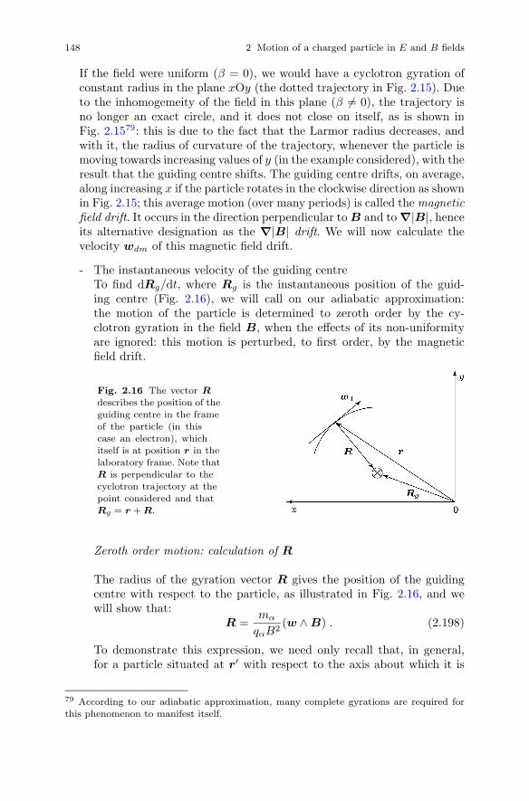
148 2 Motion of a charged particle in E and B fields
If the field were uniform (β = 0), we would have a cyclotron gyration ofconstant radius in the plane xOy (the dotted trajectory in Fig. 2.15). Dueto the inhomogemeity of the field in this plane (β �= 0), the trajectory isno longer an exact circle, and it does not close on itself, as is shown inFig. 2.1579: this is due to the fact that the Larmor radius decreases, andwith it, the radius of curvature of the trajectory, whenever the particle ismoving towards increasing values of y (in the example considered), with theresult that the guiding centre shifts. The guiding centre drifts, on average,along increasing x if the particle rotates in the clockwise direction as shownin Fig. 2.15; this average motion (over many periods) is called the magneticfield drift. It occurs in the direction perpendicular toB and to∇|B|, henceits alternative designation as the ∇|B| drift. We will now calculate thevelocity wdm of this magnetic field drift.
- The instantaneous velocity of the guiding centreTo find dRg/dt, where Rg is the instantaneous position of the guid-ing centre (Fig. 2.16), we will call on our adiabatic approximation:the motion of the particle is determined to zeroth order by the cy-clotron gyration in the field B, when the effects of its non-uniformityare ignored: this motion is perturbed, to first order, by the magneticfield drift.
Fig. 2.16 The vector R
describes the position of theguiding centre in the frame
of the particle (in thiscase an electron), which
itself is at position r in thelaboratory frame. Note that
R is perpendicular to thecyclotron trajectory at the
point considered and thatRg = r +R.
Zeroth order motion: calculation of R
The radius of the gyration vector R gives the position of the guidingcentre with respect to the particle, as illustrated in Fig. 2.16, and wewill show that:
R =mα
qαB2(w ∧B) . (2.198)
To demonstrate this expression, we need only recall that, in general,for a particle situated at r′ with respect to the axis about which it is
79 According to our adiabatic approximation, many complete gyrations are required forthis phenomenon to manifest itself.

2.2 Analysis of particular cases of E and B 149
rotating with a frequency ω, the tangential velocity obeys w = ω ∧ r′.In the present case, this translates into:
w = +qαB
mα∧R . (2.199)
Multiplying this expression vectorially on the right by B, yields:
w ∧B =qαmα
(B ∧R) ∧B . (2.200)
Recalling that the double vectorial product obeys the following rule:
P ∧ (Q ∧ T ) = Q(T · P )− T (P ·Q) , (2.201)
hence:(Q ∧ T ) ∧ P = T (P ·Q)−Q(T · P ) , (2.202)
we find that:
w ∧B =qαmα
[R(B ·B)−B(R ·B)] , (2.203)
where the term R ·B is zero, because to zeroth order the vector radiusof gyration R is necessarily perpendicular to the guiding axis. Then(2.203) leads to (2.198)80:
R =mα
qαB2(w ∧B) . (2.198)
First order motion: calculation of Rg
We have assumed till now that the lines of force are rectilinear. In orderto avoid repeating the calculation when tackling point 2) where the linesare curvilinear, we set B = BeB rather than B = Bez, where eB isthe unit vector tangent to the field line, which takes into account thepossible curvature of these lines.Following Fig. 2.16:
Rg = r +R , (2.204)
where R describes the guiding centre motion in the frame of the parti-cle, which is itself at position r in the laboratory frame. We can thenrewrite R (2.198) in the form:
R =mα
qαB(w ∧ eB) . (2.205)
80 In fact, it is sufficient to note that |R| = mαw⊥/qαB (|R| = rB) and that R isperpendicular to w and B.

150 2 Motion of a charged particle in E and B fields
The derivative of (2.204), taking (2.205) into account, gives81:
dRg
dt=
dr
dt+
dR
dt= w − mα
qαB2
dB
dt(w ∧ eB)
+mα
qαB
(dw
dt∧ eB
)
+mα
qαB
(
w ∧ deBdt
)
,
(2.206)
where deB/dt = 0 when we assume that B is directed parallel to thez axis (case 1). In the context of point 2) which follows, where wemake the assumption of a weak field curvature, we will neglect the termcomprising deB/dt
82. We can therefore take B = ezB and (2.206)reduces to:
dRg
dt= w − mα
qαB3
dB
dt(w ∧B) +
mα
qαB2
(dw
dt∧B
)
. (2.207)
In order to modify the third term on the RHS, we will take the equa-tion of motion mαdw/dt = qα(w ∧ B) and multiply it on the rightvectorially by B:
mαdw
dt∧B = qα(w ∧B) ∧B . (2.208)
Owing to the properties of the double vectorial product (2.199):
(w ∧B) ∧B = B(B ·w)−w(B ·B) ≡ B(Bw‖)−wB2 , (2.209)
we obtain:
mαdw
dt∧B = qα(w‖ −w)B2 . (2.210)
This expression can be substituted in the third term on the RHS of(2.207), which after some reorganisation, becomes:
dRg
dt= w +
1
qαB2
[qα(−w +w‖)B
2]− mα
qαB3
dB
dt(w ∧B) . (2.211)
After simplification, we find an expression for the (instantaneous) ve-locity of the guiding centre in the laboratory frame:
dRg
dt= w‖ −
mα
qαB3
dB
dt(w⊥ ∧B) , (2.212)
81 If B is spatially non-uniform in the laboratory frame, it varies with time in the frame
of the particle, as already mentioned.82 If we include the term deB/dt, its contribution will be of second order in an expressionwhich is of first order. In effect, deB/dt = (∂eB/∂y)∂y/∂t is a second order term.

2.2 Analysis of particular cases of E and B 151
where the first term represents the guiding centre velocity along thelines of force of the field B (zeroth order expression) and the secondterm is that in the direction perpendicular to w⊥ and B (first orderexpression), a motion that varies with time as a result of the cyclotrontrajectory of the particle.
- The average velocity of the guiding centre in the plane perpendicularto w⊥ and to B: the gradient of the magnetic field drift velocityIn order to calculate the temporal average of the second term on theRHS of (2.212), we rearrange it in the following form:
−mα
qαB3
dB
dt(w ∧B) =
−mα
qαB3
∂B
∂ywy (wxex + wyey + wzez) ∧Bzez
=−mα
qαB3
∂B
∂ywy(exwyBz − eywxBz) , (2.213)
where the RHS is now expressed in the laboratory frame. Since thetemporal average of wxwy is zero83 and that:
w2y =
1
2w2
⊥ , (w2⊥ ≡ w2
x + w2y) , (2.214)
the velocity associated with the average motion of the magnetic fielddrift finally reduces to:
wdm =−mα
qαB2
∂B
∂y
w2⊥2
ex . (2.215)
This expression can be transformed, since in a direct trihedral coordi-nate system (contrary to a indirect one) −ex = ez ∧ ey, into:
wdm = mαw2
⊥2
1
qαB3(B ∧∇B) (2.216)
or, equivalently:
wdm =μ
qα
(B ∧∇B)
B2, (2.217)
which is the magnetic field drift velocity of a particle in the presenceof a gradient in the field perpendicular to B and assumed to have nocurvature84.The relation (2.217) could have been obtained directly from the gen-eral expression giving the drift velocity of charged particles subjectedto a magnetic field in the presence of a given force, as is shown in Ap-
83 Larmor motion: if wx is proportional to sinωct and wy is proportional to cosωct, sincethese two functions are orthogonal, the time integral of wxwy over a period is zero.84 In fact, this gradient is related to the lines of force because β � 1/ρ (XIII.18).

152 2 Motion of a charged particle in E and B fields
pendix XII. Appendix XIII allows us, in addition, to write (2.217) inthe form:
wdm = − 1
ωcB
w2⊥2
(ρ
ρ2∧B
)
, (2.218)
where ρ is the radius of curvature (see Fig. XIII.1). It will be useful tocompare this expression with that of the curvature drift velocity, whichwe will now calculate.
2. Accounting for the curvature of the field linesThe magnetic field drift, for which we have just established the equationsof motion, cannot exist alone, because the lines of force of B which wehave supposed to be rectilinear by setting:
B = ezB0(1 + βy) , (2.219)
where β � 1, are not really so! In fact, although Maxwell’s equation forthe divergence of B:
∇ ·B ≡ ∂Bx
∂x+
∂By
∂y+
∂Bz
∂z= 0 (2.220)
can be trivially verified, in contrast to Maxwell’s equation ∇ ∧B = 085,since the curl operates on (2.219). It requires that the field B be in theform:
B = ey(βB0z) + ez[B0(1 + βy)] , (2.221)
as is shown in (XIII.7). Note that the component along y is of first order(β � 1). These field lines, which we find in a toroidal configuration, areschematically drawn in Fig. 2.17: the greater the distance from the originof the frame, the more the contribution from By becomes important.
Fig. 2.17 Lines of forcey(z) in the presence of a
gradient in B in the direc-tion perpendicular to B.
85 In general ∇∧H = J + ε0∂E/∂t: however, in the context of the individual trajectoriesmodel, we neglect the current associated with the charged particle motion, J = 0, as well
as the corresponding displacement current ε0∂E/∂t. This last term is non zero in the caseof a variable electric field E applied from outside.

2.2 Analysis of particular cases of E and B 153
The expression (2.221) represents a fieldB with lines of force characterisedby a local curvature ρ. Recalling that the radius of curvature at a givenpoint A of a curve is the distance between that point and the point ofintersection of two normal vectors to the curve situated immediately oneither side of A (Fig. XIII.1 of Appendix XIII), one can show that ρ isapproximately 1/β (XIII.18).
- Magnetic curvature drift velocityThis field curvature is associated with a particular drift motion, per-pendicular to the lines of force (hence a velocity perpendicular to B,as with the other drift velocities already defined). We will determinethe average temporal velocity of this drift called the magnetic cur-vature drift , by resorting to the general expression for the drift of acharged particle subject to a given force FD in a magnetic field B(Appendix XII).For this, we need to know the expression for the force exerted on theparticle by the curvature of the lines: during its helical motion aroundthe lines of force, the particle experiences a centrifugal force, for whichthe corresponding inertia term is of the classical form:
F cd = −mαw
2‖
ρey , (2.222)
where w‖ is the velocity parallel to the line of B at a given point andey is the base vector linked to the coordinate system of the particle anddirected towards the “instantaneous centre of rotation”: we then haveρ = −ρ ey. Following (XII.2), the drift velocity in the curved magneticfield is then:
wdc =mαw
2‖
qαρ2B2ρ ∧B (2.223)
or equivalently:
wdc = −w2
‖
ωc
ρ ∧B
ρ2B. (2.224)
- Total drift velocity due to the presence of a gradient in B in the directionperpendicular to BFrom (2.218) and (2.224), we obtain finally:
wdm +wdc = − ρ ∧B
Bωcρ2
[1
2w2
⊥ + w2‖
]
.
↑ ↑ ↑Chargesign
Magneticfield drift
Magneticcurvature drift
(2.225)
Remark: These two contributions to the drift motion are in the samedirection, defined by the vector −ρ ∧ B, but whose sense depends
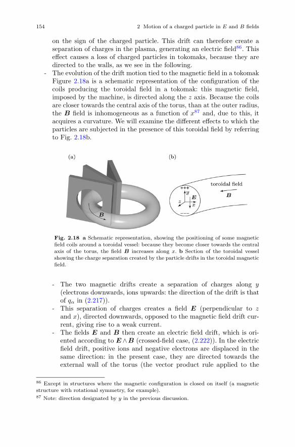
154 2 Motion of a charged particle in E and B fields
on the sign of the charged particle. This drift can therefore create aseparation of charges in the plasma, generating an electric field86. Thiseffect causes a loss of charged particles in tokomaks, because they aredirected to the walls, as we see in the following.
- The evolution of the drift motion tied to the magnetic field in a tokomakFigure 2.18a is a schematic representation of the configuration of thecoils producing the toroidal field in a tokomak: this magnetic field,imposed by the machine, is directed along the z axis. Because the coilsare closer towards the central axis of the torus, than at the outer radius,the B field is inhomogeneous as a function of x87 and, due to this, itacquires a curvature. We will examine the different effects to which theparticles are subjected in the presence of this toroidal field by referringto Fig. 2.18b.
Fig. 2.18 a Schematic representation, showing the positioning of some magnetic
field coils around a toroidal vessel: because they become closer towards the centralaxis of the torus, the field B increases along x. b Section of the toroidal vessel
showing the charge separation created by the particle drifts in the toroidal magneticfield.
- The two magnetic drifts create a separation of charges along y(electrons downwards, ions upwards: the direction of the drift is thatof qα in (2.217)).
- This separation of charges creates a field E (perpendicular to zand x), directed downwards, opposed to the magnetic field drift cur-rent, giving rise to a weak current.
- The fields E and B then create an electric field drift, which is ori-ented according to E ∧B (crossed-field case, (2.222)). In the electricfield drift, positive ions and negative electrons are displaced in thesame direction: in the present case, they are directed towards theexternal wall of the torus (the vector product rule applied to the
86 Except in structures where the magnetic configuration is closed on itself (a magneticstructure with rotational symmetry, for example).87 Note: direction designated by y in the previous discussion.
Problems 155
right trihedral coordinate system yields −ey ∧ ez = −ex). Thesecharged particles are then “lost” to the fusion plasma: they recom-bine at the wall losing their energy, additionally inflicting damageon the wall.
Remark: The plasma particles subjected to a simple toroidal magneticfield do not remain confined, as we have just seen, and a supplemen-tary magnetic field, called a “poloidal” field, is used to reduce the drifteffects. This second magnetic field provides a slight azimuthal variationto the toroidal magnetic field line configuration, forming a helix aroundthe minor axis of the torus, in order to prevent particles from travelingto the walls.
Problems
2.1. Consider electrons and ions, of mass me and mi respectively, subjectto a constant electric field. Assuming that the average time τ between twocollisions is the same for electrons and ions, show that the (average) kineticenergy acquired by an electron in the time τ is mi/me times greater thanthat acquired by an ion in the same time.
Answer
We know that:
F ≡ |q|E = medwe
dt= mi
dwi
dt. (2.226)
The same force, with opposite sign, acts on the ion and the electron. Fromthis, for a time τ between two collisions:
τ∫
0
F dt = me[we(τ)− we(0)] , (2.227)
= mi[wi(τ)− wi(0)] , (2.228)
and, to simplify the problem, setting we(0) = wi(0) = 0, we obtain:
we =mi
mewi . (2.229)
The ratio of the kinetic energy of the electron to that of the ion is then:

156 2 Motion of a charged particle in E and B fields
EceEci
=mew
2e/2
miw2i /2
=
me
(mi
me
)2
w2i
miw2i
=mi
me! (2.230)
2.2. Consider the motion of an electron (α = e) or that of an ion (α = i) inthe plane perpendicular to a magnetic field B = Bez present in the plasma,as shown in Fig. 2.4.
a) Calculate the direction and amplitude of the magnetic moment μα of anelectron and an ion in cyclotron rotation about B.
b) Calculate the macroscopic magnetisation Mα (magnetic moment per unitvolume, expressed in A/m) induced by the electron (α = e) and ion (α = i)populations rotating in the field B:
Mzα =
∫
μzαfα(w) dw . (2.231)
Assume that the velocity distributions fα(w) for the electrons and ionsare Maxwellian, with temperatures Te and Ti, respectively.
c) Calculate the total macroscopic magnetisation M and discuss the respec-tive contributions of the electron and ion populations to the plasma dia-magnetism.
d) Assuming that ne = ni = n and Te = Ti = T , deduce the magnetic in-duction B resulting from both the applied magnetic induction B0 = B0ezand the component μ0M due to the diamagnetism of the plasma. Writethe condition for which the intensity of the field B in the plasma becomesequal to half B0.
Numerical application: B0 = 2× 10⁻² tesla (200 gauss), Te = Ti = 35000K.
Answer
a) The cyclotron motion of an electron and an ion in the plane perpendicularto the magnetic induction B can be described by equation (2.68):
wα = ωcα ∧ rBα (2.232)
where:
ωcα = −qαB
mα. (2.233)
For the electrons, ωce and B are collinear with the same sign, i.e. thesame direction, while for the ions, ωci and B have opposite sign. On theother hand, the currents ie and ii associated with the cyclotron motionof electrons and ions are in the same direction, because of their oppositecharge, as shown in the Fig. 2.4. They induce a magnetic field B′ in the

Problems 157
Fig. 2.19 Characteristic parameters of the cyclotron motion of an electron (left) and
an ion (right) in a magnetic field.
direction opposite to B (Biot-Savart Law (2.70)); for the same reasons, μi
and μe are anti-parallell to B, as shown in Fig. 2.19.The modulus of the magnetic moment μ is defined as the product of acurrent density i circulating in a closed loop with surface S. In the case ofa cyclotron gyration:
μzα = πr2Bαiα . (2.234)
The current induced by the rotational motion is then:
iα =qαωcα
2π, (2.235)
such that (2.148):
μzα =mαw
2⊥α
2B. (2.236)
b) For an ensemble of particles of type α, the average value Mz of the macro-scopic magnetisation (in the hydrodynamic sense) is given by (3.39):
Mzα =
∫
w
μzfα(w) dw , (2.231)
i.e. (neglecting the subscript α):
Mz =1
B
∫
w
mw2⊥
2n
(m
2πkBT
) 32
exp
(
− mw2
2kBT
)
dw , (2.237)
which can be expanded:

158 2 Motion of a charged particle in E and B fields
Mz =nm
2B
(m
2πkBT
) 32
⎡
⎣
∞∫
−∞
w2x exp
(
− mw2x
2kBT
)
dwx
×∞∫
−∞
exp
(
−mw2
y
2kBT
)
dwy
∞∫
−∞
exp
(
− mw2z
2kBT
)
dwz
+
∞∫
−∞
exp
(
− mw2x
2kBT
)
dwx
∞∫
−∞
w2y exp
(
−mw2
y
2kBT
)
dwy
×∞∫
−∞
exp
(
− mw2z
2kBT
)
dwz
⎤
⎦ (2.238)
and this reduces to:
Mzα =nαkBTα
B. (2.239)
In vector form, taking account of the sense of the induced magnetisationMα with respect to B:
Mα = −nαkBTα
B2B . (2.240)
c) The total magnetisation is the sum of those induced by the ions and theelectrons, i.e.:
M = − B
B2(nekBTe + nikBTi) . (2.241)
If Ti � Te, M is induced solely by the electrons.If Ti = Te, the contribution from the ions is equal to that from the elec-trons.
d) For ne = ni = n and Te = Ti = T , we have from (2.241):
M = −2nkBT
B2B = − 2p
B2B , (2.242)
where p is the pressure exerted by the charged particles, referred to as the(scalar) kinetic pressure (p. 205).B is the magnetic induction in the plasma and results from the vectoraddition of the applied field B0 (which exists in the absence of the plasma)and the field created by the motion of charged particles, i.e. μ0M (themagnetisation M giving the magnetic field, the corresponding magneticinduction is thus obtained by multiplying the field M by μ0, the vacuummagnetic permeability). We then have:

Problems 159
B = B0 + μ0M =B0 −p
B2/2μ0B , (2.243)
B
(
1 +p
B2/2μ0
)
=B0 . (2.244)
The diamagnetism of the plasma causes a reduction of the applied mag-netic field, due to the motion of the charged particles in the same field.The diamagnetism can be neglected (B � B0) if:
p � B2
2μ0, (2.245)
i.e. the kinetic pressure p remains much smaller than themagnetic pressureB2/2μ0.The magnetic induction in the plasma is half the applied magnetic field(B = B0/2) if:
p =B2
2μ0, (2.246)
that is:
n =B2
2μ0kBT. (2.247)
Numerical application
From (2.247), we obtain:
n =10−4
2× 4π × 10−7 × 1.38× 10−23 × 35000= 8.24× 10¹⁹ m−3 ,
= 8.24× 1013 cm−3 . (2.248)
Remark: Maxwell’s Law for the curl of H applied to the field M leads toJM = ∇ ∧M. Since M is uniform in the plasma:
∇ ∧M = 0 , (2.249)
thus JM = 0: no macroscopic current is induced. On the other hand, inregions with gradients in M (boundaries of enclosed plasmas), the diamag-netism of the plasma actually induces magnetisation currents (JM �= 0).
2.3. Consider a particle of charge q subject to uniform, static magnetic andelectric fields which are perpendicular to each other. The particle velocity wcan be decomposed according to w = wD+w′, where wD is the electric fielddrift. From the equation of motion, show analytically that w′ represents themotion the particle would have in the magnetic field alone.

160 2 Motion of a charged particle in E and B fields
Answer
The equation of motion can be written (2.5):
mdw
dt= q [E⊥ +w ∧B] (2.250)
in which we substitute wD +w′ for w knowing that:
wD =E⊥ ∧B
B2, (IX.2)
noting that dwD/dt = 0 because E and B are constant in time. We find:
mdw′
dt= q
[
E⊥ +
(E⊥ ∧B
B2
)
∧B +w′ ∧B
]
. (2.251)
From the double vector product:
(Q ∧ T ) ∧ P = T (P ·Q)−Q(T · P ) , (2.252)
this becomes:(E ∧B
B2
)
∧B =B(B ·E)−E(B2)
B2= −E
B2
B2(2.253)
from the assumption that E is perpendicular to B.Finally:
dw′
dt= q(w′ ∧B) , (2.254)
which is precisely the motion of a particle in a magnetic field alone.
2.4. Consider the motion of a charged particle in a uniform and static mag-netic field B, and a uniform electric field E, directed perpendicular to B andslowly varying in time. The velocity of the particle is denoted by w.
a) Show, by expressing the velocity w in terms of the following three velocitycomponents:
w = wD +w′ +wp , (2.255)
where wD is the electric field drift velocity and:
wp =m
qB2
∂E
∂t, (2.256)
that w′ and wp then obey the equation of motion:
mw′ +mwp = q(w′ ∧B) , (2.257)
where m is the mass of the particle and q its charge.

Problems 161
b) Consider a periodically varying field E(t), with an angular frequency ω.Show that if the frequency of the field oscillation is small compared to ωc
for the cyclotron gyration, then the w′ component describes the cyclotronmotion of the particle in the B field alone.
c) Show that there is no net current (ions and electrons) associated with wD
while, on the other hand, wp leads to a current which is referred to as thepolarisation current:
Jp =ρmB2
E , (2.258)
where ρm = (me +mi)n is the mass density of the electrons and ions (ofmasses me and mi respectively) and n, the charged particle density. Thevelocity wp is called the polarisation drift velocity.
d) By considering the total charge current (the conduction current and thedisplacement current ∂D/∂t), show that the relative permittivity of themedium with respect to vacuum is given by:
εp = 1 +ρmε0B2
. (2.259)
To do this, recall from (2.45) that:
JT =∂D
∂t+ Jc =
∂D′
∂t, (2.260)
where D′ = ε0εpE is the displacement current in the dielectric description(see (2.43)).
Answer
a) Equation (2.257) signifies that the presence of the field E does not quali-tatively modify the helical motion (described by w′: to be shown in b) ofthe particle.We know that the equation of motion is linked to the Lorentz force by:
mw = q[E +w ∧B] , (2.261)
independent of the form of E and B.In the present case, we make the assumption that the total velocity canbe expressed in terms of the three vectors given by (2.255). Developing(2.261) in terms of these different velocities, we obtain:
mwD +mw′ +mwp = q[E + (wD ∧B) + (w′ ∧B) + (wp ∧B)] (2.262)
and, replacing wp on the RHS by equation (2.256) and wD by its vectorform:
wD =E ∧B
B2, (2.263)

162 2 Motion of a charged particle in E and B fields
we obtain:
mwD +mw′ +mwp = q
⎧⎨
⎩E +
⎡
⎣(E ∧B
B2
)
∧B
︸ ︷︷ ︸
⎤
⎦+ (w′ ∧B)
double vector product−E
+m
q
d
dt
(E ∧B
B2
)
︸ ︷︷ ︸
⎫⎬
⎭. (2.264)
= mwD
From the double vector product (see problem 2.3), this becomes:
mwD +mw′ +mwp = q {E −E + (w′ ∧B)}+mwD (2.265)
and finally:
mw′ +mwp = q(w′ ∧B) . (2.257)
b) We need to show, starting from (2.256) and (2.257), that∣∣wp/w
′∣∣ � 1.Setting E = E0e
iωt, we can write:
∣∣∣∣
mwp
mw′ +mwp
∣∣∣∣ =
∣∣∣∣m2ω2
qB2E0
∣∣∣∣
∣∣∣∣
1
qw′B
∣∣∣∣
=
∣∣∣∣ω2
ω2c
∣∣∣∣
∣∣∣∣E0
Bw′
∣∣∣∣ =
∣∣∣∣ω2
ω2c
∣∣∣∣
∣∣∣wD
w′
∣∣∣ , (2.266)
which indicates that we require not only ω/ωc ≤ 1 but also, preferably,wD � w′, which is an acceptable hypothesis.
c) Since the velocity wD does not depend on the charge of the particles, thecorresponding conduction current density is zero, because:
JD =∑
α
nαqαwD = nwD(e− e) = 0 . (2.267)
For the conduction current referred to as the polarisation current, we have:
Jp ≡∑
α
nαqαwpα =E
B2
[ne(−e)me
−e+
ni(e)mi
e
]
=E
B2n(mi +me) , (2.268)
=E
B2ρm . (2.269)

Problems 163
d) The conduction current Jc reduces to Jp, as we have just shown. In addi-tion, because quite generally:
JT ≡ ∂D
∂t+ Jc =
∂D′
∂t, (2.260)
in the present case this reduces to:
JT ≡ ε0E + Jp = εpε0E (2.270)
and from (2.269):
JT ≡ ε0E +E
B2ρm = εpε0E , (2.271)
such that we obtain, as required:
εp = 1 +ρmB2ε0
. (2.259)
2.5. Consider a plasma subject to a high frequency electric field E0eiωt, di-
rected arbitrarily with respect to a static magnetic field of intensity B, bothfields being spatially uniform. In the framework of the “individual motionof charged particles” description, calculate the conductivity and permittivitytensors for electrons whose motion is associated with the particular solutionof the non-resonant equation of motion. Assume B is directed along the Ozaxis and express E⊥ in terms of the Cartesian coordinates x and y. The mul-tiplying factor for the tensor σ should be such that it reduces to a unitarymatrix for B = 0.
Answer
In order to obtain w2, the particular solution to this problem (see Sect. 2.2.2,p. 123), we used the frame of Fig. 2.10, which led us to the expression:
w2 =[aE0‖ + bE0⊥ + c(E0⊥ ∧B)
]eiωt . (2.127)
To transpose this result into Cartesian coordinates (x, y, z), as posed by thequestion, we write:
w2 = ez(aE0‖) + ex(bE0x) + ey(bE0y) + c(exE0x + eyE0y) ∧ ezB , (2.272)
where we have set E0⊥ = exE0x+eyE0y and have canceled, for simplicity, thedependence on eiωt. After regrouping the terms along the three base vectors,we find:
w2 = ex[bE0x + cE0yB] + ey[bE0y − cE0xB] + ez[aEz] . (2.273)
Including the coefficients a, b and c for the non-resonance solution fromSect. 2.2.2 (Eq. (2.135)), we obtain:

164 2 Motion of a charged particle in E and B fields
w2 = ex
[iq
mα
ω
ω2c − ω2
E0x +q2
m2α
B
ω2c − ω2
E0y
]
+ ey
[iq
mα
ω
ω2c − ω2
E0y −q2
m2α
B
ω2c − ω2
E0x
]
+ ez
[
− iq
ωmαEz
]
. (2.274)
To develop the electrical conductivity tensor, recall that J i = σijEj
(2.121). By definition, the current density J i = nqwi and we have, afterintroducing the factor −inq2/mαω:
J = − inq2
mαω
{
ex
[(
− ω2
ω2c − ω2
E0x
)
+iq
mα
ωB
ω2c − ω2
E0y
]
+ ey
[
− ω2
ω2c − ω2
E0y −iqBω
mα(ω2c − ω2)
E0x
]
+ ezEz
}
. (2.275)
There are two components of σ along ex, and recalling that qB/mα = −ωc,we find:
σxx =ω2
ω2 − ω2c
, σxy =iωcω
ω2 − ω2c
, (2.276)
then, along ey:
σyy =ω2
ω2 − ω2c
, σyx = − iωcω
ω2 − ω2c
, (2.277)
and, finally, along ez:σzz = 1 . (2.278)
The tensor σ, represented as a 3× 3 matrix, has the value:
σ = − inq2
mαω
⎛
⎜⎜⎜⎜⎜⎜⎝
ω2
ω2 − ω2c
iωcω
ω2 − ω2c
0
− iωcω
ω2 − ω2c
ω2
ω2 − ω2c
0
0 0 1
⎞
⎟⎟⎟⎟⎟⎟⎠
(2.279)
and we can verify that if B = 0 (ωc = 0), the matrix becomes unitary: theplasma is no longer anisotropic.
For the relative permittivity tensor εp, we have for E0eiωt:
εp = I +σ
iωε0, (2.125)
such that:

Problems 165
εp =
⎛
⎜⎜⎜⎜⎜⎜⎜⎜⎝
1− nq2
mε0ω2
ω2
ω2 − ω2c
− nq2
mε0ω2
iωcω
ω2 − ω2c
0
nq2
mε0ω2
iωcω
ω2 − ω2c
1− nq2
mε0ω2
ω2
ω2 − ω2c
0
0 0 1− nq2
mε0ω2
⎞
⎟⎟⎟⎟⎟⎟⎟⎟⎠
, (2.280)
from which, finally:
εp =
⎛
⎜⎜⎜⎜⎜⎜⎜⎜⎝
1−ω2pe
ω2 − ω2c
−iω2
pe
ω2 − ω2c
ωc
ω0
iω2pe
ω2 − ω2c
ωc
ω1−
ω2pe
ω2 − ω2c
0
0 0 1−ω2pe
ω2
⎞
⎟⎟⎟⎟⎟⎟⎟⎟⎠
. (2.281)
2.6. Consider a uniform, alternating electric field of the form E0e−iωt, to-
gether with a uniform, static magnetic field B along the z axis (entering intothe page). We wish to study the phenomenon of cyclotron resonance usingthe coordinate frame rotating in the plane perpendicular to B. Expressingthe field E in the laboratory Cartesian frame in the form:
E = exEx + eyEy + ezEz , (2.282)
the same field in the rotating coordinates frame is written:
E =e+E+ + e−E− + ezEz
=(ex + iey)√
2E+ +
(ex − iey)√2
E− + ezEz . (2.283)
a) Express the components E+ and E− in terms of the components Ex andEy. Determine which of the two unit vectors, e+ or e−, rotate in the samedirection as the electrons during their cyclotron motion around B.
b) The conductivity tensor, expressed in the laboratory frame, for ω �= ωc,and E0e
−iωt, has the following elements (exercise 2.5):
σ = σ0
⎛
⎜⎜⎜⎜⎜⎝
ω2
ω2 − ω2c
−iωωc
ω2 − ω2c
0
iωωc
ω2 − ω2c
ω2
ω2 − ω2c
0
0 0 1
⎞
⎟⎟⎟⎟⎟⎠
. (2.284)
166 2 Motion of a charged particle in E and B fields
Show, by calculating the corresponding terms σ+ and σ−, that this tensoris diagonalised in the rotating frame.
c) Show that electron cyclotron resonance leads to an increase in velocity ofthe particles as a function of time, according to the relation:
w2 =q
mE+t . (2.285)
In other words, the electrons in their own frame “see” a continuous electricfield (ω = 0) which accelerates them continuously between two collisions.For this, develop the relation (2.146) in the laboratory frame.
Answer
a) We can develop (2.283) by regrouping the terms along the unit vectors inthe laboratory frame:
E =1√2ex[E+ + E−] +
i√2ey[E+ − E−] + ezEz , (2.286)
which must be equal to the same vector E expressed in the laboratoryframe:
E = exEx + eyEy + ezEz , (2.287)
from which:
Ex =1√2[E+ + E−] , (2.288)
Ey =i√2[E+ − E−] . (2.289)
By combining (2.288) and (2.289), we obtain the components of the fieldE in the rotating frame:
E+ =Ex − iEy√
2(2.290)
and, similarly:
E− =Ex + iEy√
2. (2.291)
The components E+ and E−, in terms of the components Ex and Ey,thus correspond to the concept of a rotating field: the superposition of twooscillating fields with the same frequency, perpendicular to each other andin phase quadrature.Since the rotating field E+ can be written:
E+ =ex + iey√
2E+e
−iωt , (2.292)

Problems 167
taking the real part, we obtain:
E+ =E+√2(ex cosωt+ ey sinωt) , (2.293)
from which it is easy to verify, in the xOy plane, that the vector e+ (andthus the field E+) rotates in the clockwise direction, thus, according to ourconvention (field B entering the page and ωc > 0), in the same direction asthe electrons, as shown in the figure. Note that the intensity in expression(2.293) originating from (2.290), is constant in the rotating frame.Make sure that the orientation of the axes x and y is such that the fieldalong z enters into the page (right-handed frame).
b) Equation (2.284) gives us the components of the tensor in the laboratoryframe. Note that σxx = σyy and σxy = −σyx. Thus, by expanding thecurrent density J = σ ·E in the laboratory frame, we can write:
σ ·E = σxxexEx + σxyexEy − σxyeyEx + σxxeyEy + σzz ezEz . (2.294)
Replacing the components of the fields in the laboratory frame with thoseof the rotating frame ((2.288) and (2.289)), we have:
σ ·E = σxxex1√2[E+ + E−] + σxyex
i√2[E+ − E−] (2.295)
− σxyey1√2[E+ + E−] + σxxey
i√2[E+ − E−] + σzz ezEz .
Regrouping the terms in E+ and those in E−:
E+√2[ex σxx + iex σxy − ey σxy + iey σxx] , (2.296)
E−√2[ex σxx − iex σxy − ey σxy − iey σxx] , (2.297)
and introducing the base vectors e+ and e−, we find:
E+
[ex + iey√
2σxx + i
ex + iey√2
σxy
]
+
E−
[ex − iey√
2σxx − i
ex − iey√2
σxy
]
. (2.298)
Finally, we obtain:
σ ·E = E+e+σxx+iE+e+σxy+E−e−σxx−iE−e−σxy+σzz ezEz . (2.299)
We can now introduce the elements of the tensor σ in the rotating frame:
168 2 Motion of a charged particle in E and B fields
σ ·E =[E+e+(σxx + iσxy
︸ ︷︷ ︸σ+
) + E−e−(σxx − iσxy︸ ︷︷ ︸
σ−
)]+ σzz ezEz , (2.300)
which is an expression showing that, in the rotating frame, the tensor hasbeen diagonalised (there are no mixed components E+e− or E−e+). Thematrix can now be represented by:
σ = σ0
⎛
⎜⎜⎝
ω
ω − ωc0 0
0ω
ω + ωc0
0 0 1
⎞
⎟⎟⎠ , (2.301)
where the base vectors are e+, e− and ez, respectively.We can thus verify that the electron resonance is indeed directed along e+(ω = ωc).
c) Consider (2.146):
w2 =
[
− iqαmαω
E0‖ +qα
2mαω(ωt− i)E0⊥ − iq2αt
2ωm2α
(E0⊥ ∧B)
]
eiωt ,
(2.302)where we have replaced the dependence eiωt of the field E by e−iωt, asindicated in the introduction.We will replace i by −i in (2.302). Since we are only interested in theresonance phenomenon, we will ignore the term in the ez direction and thesecond term in E0⊥, which is time independent (which rapidly becomesnegligible). Writing this in Cartesian coordinates:
E0⊥ = exE0x + eyE0y , (2.303)
this becomes:
w20⊥ =qt
2m(exE0x + eyE0y) +
iq2Bt
2ωm2(exE0y − eyE0x) . (2.304)
Knowing that at resonance, −qB/m = ωc and ω = ωc, from (2.304):
w20⊥ =qt
2m[(exE0x + eyE0y)− i(exE0y − eyE0x)] , (2.305)
w20⊥ =qt
2m[ex(E0x − iE0y) + ey(E0y + iE0x)] , (2.306)
w20⊥ =qt
m
[(ex + iey
2
)
(E0x − iE0y)
]
, (2.307)
such that, from (2.283) and (2.290), and multiplying by e−iωt:
w2⊥ =qt
mE+
(ex + iey√
2
)
e−iωt =qt
me+E+e
−iωt =qt
mE+ . (2.308)

Problems 169
2.7. Consider a homogeneous, static magnetic field B = ezB0 and a homo-geneous alternating electric field E = exE0 cosωt (ex, ey and ez are the unitvectors along the Cartesian axes x, y and z).
a) Show that at cyclotron resonance, the contribution of this effect to thevelocity of particles of mass m is given by:
w =q
2mE0t [cos(ωt)ex + sin(ωt)ey] +
q
2mωE0 sin(ωt)ex . (2.309)
b) Write the form of this motion at resonance explicitly. What does it repre-sent?
c) In an alternating electric field E directed instead along ey:
E = E0 sin(ωt)ey , (2.310)
show that the contribution to the particle velocity at cyclotron resonancecan be written in the form:
w′ =q
2mE0
(t− π
2ω
)[sin(ωt)ey + cos(ωt)ex]−
q
2mωE0 cos(ωt)ey .
(2.311)d) A rotating electric field is applied in the xOy plane with an amplitude such
that Ex = Ey = E0. Following the chosen direction of rotation, we have:
E+ = E0 [cos(ωt)ex + sin(ωt)ey] (2.312)
or:E− = E0 [cos(ωt)ex − sin(ωt)ey] . (2.313)
Based on the expressions for w and w′, calculate the resultant velocityfor a particle at cyclotron resonance ωc > 0 in a field rotating to the right(E+) and then a field rotating to the left (E−). What can you conclude?
Answer
a) In the presence of a magnetic field:
B = B0ez (2.314)
and in a periodic electric field perpendicular to it:
E = E0eiωtey , (2.315)
the particular solution (2.146) of the equation of motion at ω = ωc repre-sents the effect of the cyclotron resonance on the particle velocity. We willignore the contribution to the velocity in the direction parallel to the fieldB, since it is not affected by the field E, because it is perpendicular to B.

170 2 Motion of a charged particle in E and B fields
In the xOy plane (2.142) we have:
w2 =
[q
2mω(ωt− i)E0ex − iq2t
2ωm2(E0ex ∧B0ez)
]
eiωt . (2.316)
We can then take the real part of this expression (knowing that eiωt =cos(ωt) + i sin(ωt)), from which:
w2 =q
2mωωtE0 cos(ωt)ex +
q
2mωE0 sin(ωt)ex
+q2t
2ωm2E0 sin(ωt)(ex ∧ ez)B0 . (2.317)
Since ex ∧ ez = −ey (right-handed frame) and ω = ωc ≡ −qB0/m, thisbecomes:
w2 =q
2mE0t
[
cos(ωt)ex − qm
(−1)qB0msin(ωt)B0ey
]
+q
2mωE0 sin(ωt)ex . (2.318)
By setting w2 = w, we obtain the relation from statement a):
w =q
2mE0t[cos(ωt)ex + sin(ωt)ey] +
q
2mωE0 sin(ωt)ex . (2.309)
b) The third term on the RHS of (2.309) describes a periodic motion in thedirection of the field E (this is normal: it would also exist in the absenceof B) while the first and the second conjugate terms represent a periodicrotational motion, of frequency ωc, whose amplitude continuously increaseswith time: in other words, the particle describes a spiral. The modulus ofthe corresponding velocity of this motion is w0 = qE0t/2m, because thecontribution to the periodic motion along ex rapidly becomes negligible.This increase in amplitude comes precisely from the resonance between ωand ωc, called cyclotron resonance.
c) We use equation (2.317), in which the direction of the field E is along eyrather than ex. Since ey ∧ ez = ex, we have:
w′ =qt
2mE0 cos(ωt)ey +
q
2mωE0 sin(ωt)ey +
q2t
2ωm2E0B0 sin(ωt)ex
=q
2mE0t [cos(ωt)ey − sin(ωt)ex] +
q
2ωmE0 sin(ωt)ey . (2.319)
We now change the time origin by replacing t by t−π/2ω: as cos (ωt− π/2)= sin(ωt) and sin (ωt− π/2) = − cos(ωt), we obtain from (2.319):

Problems 171
w′ =q
2mE0
(t− π
2ω
)[sin(ωt)ey + cos(ωt)ex]
− q
2mωE0 cos(ωt)ey . (2.311)
d) To get the resulting particle velocity in the field E+ (defined by (2.312)),we simply add the velocities w +w′ from equations (2.309) and (2.311):
wTOT+ =q
2mE0t[2 cos(ωt)ex + 2 sin(ωt)ey] (2.320)
−qE0π
4mω[sin(ωt)ey + cos(ωt)ex] +
qE0
2mω[sin(ωt)ex − cos(ωt)ey] .
To obtain the resulting particle velocity in the field E−, we add the velocityw with w′′, where w′′ = −w, since then E = −E0 sin(ωt)ey. This yields:
wTOT– ≡ w −w′
=q
2mE0t [
= 0︷ ︸︸ ︷cos(ωt)ex + sin(ωt)ey − sin(ωt)ey − cos(ωt)ex ]
+q
4m
π
ωE0[sin(ωt)ey + cos(ωt)ex]
+q
2mωE0[sin(ωt)ex + cos(ωt)ey] . (2.321)
We can conclude that if the field turns in the positive direction of ωc (i.e.if the particle velocity is not in the direction of the rotating field), thevelocity of the particle does not increase linearly in time and, therefore,there is no cyclotron resonance.
2.8. Consider a magnetic field of the form:
B = B0(1− ε cos kx)ex , (2.322)
where ε is a parameter smaller than unity and k is a constant. This fieldis used to axially confine charged particles at each end of a linear machinewhose centre is at x = 0.
a) Find the expression for w‖ as a function of w‖(0), w⊥(0), ε and k.b) Show that particles will be effectively trapped if:
w2‖(0) ≤ w2
⊥(0)2ε
1− ε. (2.323)
c) Assuming an isotropic velocity distribution at x = 0, calculate the numberof trapped particles as a fraction of the total number of particles.

172 2 Motion of a charged particle in E and B fields
Answer
a) This is a case in which the magnetic field has a (weak) non uniformity inits own direction, which corresponds to the situation treated in Sect. 2.2.3(page 138); note that we are using here the x axis as the direction of Brather than z. We know that the expression:
B = B0(1− ε cos kx)ex (2.324)
is not complete, because the component of B (of order 1), required to sat-isfy Maxwell’s equation ∇ ·B = 0, is missing. Nevertheless, this correctiondoes not appear in the calculation of the w‖ component. Finally, note thatthe minimum value of |B|, |B| = B0(1 − ε) is found at x = 0 and thuscorresponds to the region situated between the mirrors: correctly speak-ing, there is no region of uniform field in this machine, only two mirrorsat each end with a minimum in the magnetic field in between.By transposing equation (2.176) along ex and setting B‖ = B(x = 0),we have:
w‖(t) = w‖(0)−ex2r2Bω
2c
1
B(x = 0)
(∂Bx
∂x
)
y=z=0
t , (2.325)
where ωc corresponds to the value at B(x = 0). Since ∂Bx/∂x =B0εk sin kx and r2Bω
2c = w2
⊥(0), we find:
w‖(t) = w‖(0)−ex2w2
⊥(0)εk sin kx
1− εt (2.326)
(we could neglect the parameter ε compared to 1 in the denominator).b) We have shown in Sect. 2.2.3 (p. 138) that the particles coming from
the central region of the machine (x = 0) are reflected by the magneticmirror if the angle α0 of their vector velocity with respect to the axis(of components w0‖ = w0 cosα0 and w0⊥ = w0 sinα0) in the section ofuniform field (the region of the weakest field between the two mirrors) hasa value greater than α0m, defined by (2.189):
sinα0m =
√B(x = 0)
Bmax. (2.327)
Bmax is reached for cos kx = −1, from which Bmax = 1 + ε and B(x =0) = 1− ε, such that (2.327) gives:
sin2 α0m =1− ε
1 + ε. (2.328)
Noting that the ratio of the velocities w⊥(x = 0)/w(x = 0) corresponds tosinα0m, we have:

Problems 173
w2⊥(0)
w2(0)=
1− ε
1 + ε, (2.329)
such that:w2
⊥(0)(1 + ε) = (w2⊥(0) + w2
‖(0))(1− ε) , (2.330)
w2⊥(0)[(1 + ε) + (ε− 1)] = w2
‖(0)(1− ε) , (2.331)
and finally:
w2‖(0) = w2
⊥(0)2ε
1− ε. (2.332)
The condition for reflection is defined by the inequality:
w2‖(0) ≤ w2
⊥(0)2ε
1− ε. (2.333)
c) The reflection coefficient Cr of particles in a magnetic mirror (2.196)leads us to:
Cr ≡ Γr
Γinc= 1− 1
R = 1− 1
Bmax/B(x = 0)= 1− 1− ε
1 + ε=
2ε
1 + ε. (2.334)
2.9. Consider a magnetic field directed principally along z but subject to aslight curvature, represented by the term ∂Bx/∂z (we suppose that the cur-vature is in two dimensions only, in the plane xz). The origin of the Cartesianframe is chosen such that the field B is directed along the z axis while, oneach side of the origin, there is a contribution from the x and z componentsof the field, as shown in the figure. The radius of curvature ρ of this field lineis assumed to be much greater than the particle Larmor radius (of charge qand mass m).
a) Show that, in the immediate region of theorigin, B is described by:
B = B0
(
exz
ρ+ ez
)
, (2.335)
where B0 is the intensity of the field at z =0 and ex, ez are the unit base vectors in theCartesian frame (x, y, z); ρ−1 = d2x/dz2 inthe case that dx/dz is not too large.
b) Assume w is the particle velocity. Using the field given by (2.335), expressthe components of w to first order, in Cartesian coordinates.
c) Determine, to order zero, the three components of velocity and position,using the following initial conditions:
x0 = y0 = z0 = 0 , (2.336)
w0 = w⊥0ex + wz0ez , (2.337)

174 2 Motion of a charged particle in E and B fields
(the zero superscript in A0 signifies that the quantity A is expressed toorder zero).
d) Show that the calculation to first order leads to:
wx =
(w2
z0
ρ
)
t+ w⊥0 cosωct , (2.338)
wy = −(w2
z0
ρωc
)
+ w⊥0 sinωct , (2.339)
where the constants of integration are fixed such that if we set ρ−1 = 0,we will recover the zeroth order solution. In this first order calculation,we have replaced the values of wz and z, which appear in the expressionsobtained for wx and wy in b), by their values approaching z = 0, i.e. toorder zero, namely wz0 and wz0t respectively.
e) Finally, show that the position of the guiding centre satisfies the expres-sion:
x =
(1
2ρ
)
z2 . (2.340)
Answer
a) The magnetic field is directed, at the origin of the system, along the z axisand is affected by a (symmetric) curvature of the lines of force in the xOzplane. Equation (2.335) in the terms of the problem suggests that the Bx
component is a correction term for Bz in the neighbourhood of z = 0. Asimilar question was treated in Sect. 2.2.3, p. 147 and p. 152 (2.221) withthe inhomogeneity along ey instead of ex. Achieving this transpositionyields:
B = ex(βB0z) + ez[B0(1 + βx)] . (2.341)
The principal component Bz is subject to a first order correction, whichwe can neglect in comparison to B0, of order zero; the correction alongthe x axis introduces a (small) term β, where β � ρ−1 (XIII.18): equation(2.335) of the question is therefore demonstrated.We can also treat the problem from the beginning, without recourse tothe results of Sect. 2.2.3 as we have just done. Since Bx is a first ordercorrection, a development in series, limited to first order, is justified:
Bx = Bx(z = 0)︸ ︷︷ ︸
=0
+∂Bx
∂xx+
∂Bx
∂yy +
∂Bx
∂zz � ∂Bx
∂zz , (2.342)
the Bx component depending only on z (see figure). Since B = exBx +ezBz and Bz = B0, we obtain:

Problems 175
B = ex∂Bx
∂zz + ezB0 . (2.343)
To calculate ∂Bx/∂z, we consider a magnetic field line whose slope dx/dzis, as a general rule, equal to the ratio Bx/Bz of the local magnetic fieldcomponents:
dx
dz=
Bx
Bz. (2.344)
From (2.344), we have:
d2x
dz2=
∂Bx
∂z
1
Bz− ∂Bz
∂z
Bx
B2z
, (2.345)
where the second term on the RHS is negligible compared to the first termbecause it is of order 2: from (2.341) and (2.342), ∂Bx/∂z and Bx are bothnon zero only to order 1.By assumption, dx/dz is not too large in the neighbourhood of the origin,then (XIII.2):
d2x
dz2� 1
ρ. (2.346)
Finally, from (2.345) and (2.346):
∂Bx
∂z=
B0
ρ, (2.347)
from which, following (2.343), we have thus demonstrated the validityof (2.335).
b) We simply return to the general equations shown in Sect. 2.1, which wecan write, taking −qB0/m = ωc and setting E = 0 (Eqs. (2.6)–(2.8)) inthe form:
wx =q
m[Bzwy −Bywz] =
q
m[B0wy] = −ωcwy , (2.348)
wy =q
m[Bxwz −Bzwx] =
q
m
[B0z
ρwz −B0wx
]
= −ωc
[z
ρwz − wx
]
, (2.349)
wz =q
m[Bywx −Bxwy] = − q
m
[B0z
ρwy
]
= ωc
[z
ρwy
]
, (2.350)
where the underlined terms are of first order, because they tend to zero ifthe radius of curvature tends to infinity (rectilinear lines of force).
c) To obtain the expression for the components of w to order zero, we onlyneed to set ρ → ∞ in (2.348)–(2.350). We then get:

176 2 Motion of a charged particle in E and B fields
wx = −ωcwy , (2.351)
wy = ωcwx , (2.352)
wz = 0 . (2.353)
We can start by calculating the expressions for wx and x. To do this, wedifferentiate (2.351):
wx = −ωcwy (2.354)
and substituting wy from (2.352) gives:
wx = −ωc(ωcwx) , (2.355)
from which:wx + ω2
cwx = 0 , (2.356)
for which the solution is clearly:
wx = A1 cosωct+A2 sinωct , (2.357)
where A1 and A2 are constants, depending on the initial conditions (equa-tions (2.336) and (2.337)). This leads to:
wx = w⊥0 cosωct (2.358)
and:x =
w⊥0
ωcsinωct . (2.359)
To calculate the expressions for wy and y, we will take (2.352) and substi-tute therein the value of wx from (2.358). After integration, and applicationof initial conditions, we obtain:
wy = w⊥0 sinωct (2.360)
and:y =
w⊥0
ωc(1− cosωct) . (2.361)
As for wz and z, we deduce from (2.353):
wz = wz0 and z = wz0t . (2.362)
d) The system (2.348)–(2.350) can be resolved quite easily provided that, inthe terms in 1/ρ (terms of first order), the expressions for velocity andposition along ez are those of (2.362), which are of order zero. Note that,as a result, these terms remain of order one. Then from (2.349), we writedown:
wy = −ωc
[w2
z0t
ρ− wx
]
. (2.363)
Problems 177
To obtain wx, we start by differentiating (2.348):
wx = −ωcwy , (2.364)
which we can render homogeneous in wx by substituting the expressionfor wy from (2.363):
wx = ω2c
[w2
z0t
ρ− wx
]
, (2.365)
from which:
wx + ω2cwx =
ω2cw
2z0t
ρ. (2.366)
The solution is the general solution with no RHS, namely (2.358), to which
must be added a particular solution (of first order): w(1)x = w2
z0t/ρ (fol-lowing (2.366)), from which, in total:
wx = w⊥0 cosωct+w2
z0t
ρ. (2.367)
For wy, differentiate (2.363) and we have:
wy = −ωc
[w2
z0
ρ− wx
]
, (2.368)
an expression in which we can replace wx by its expression in (2.348), suchthat:
wy = −ωc
[w2
z0
ρ+ ωcwy
]
, (2.369)
from which:wy + ω2
cwy = −ωc
ρw2
z0 , (2.370)
whose solution, following the method of (2.367), is:
wy = w⊥0 sinωct−1
ρωcw2
z0 . (2.371)
e) To calculate the guiding centre velocity, we simply ignore the sinusoidalterms in (2.367) and (2.371), such that:
wx =w2
z0t
ρ, (2.372)
wy = −w2z0
ρωc, (2.373)
and, clearly (E = 0):wz = wz0 . (2.374)

178 2 Motion of a charged particle in E and B fields
The position of the guiding centre is then described by:
x =w2
z0t2
2ρ, (2.375)
y = −w2z0t
ρωc, (2.376)
z = wz0t . (2.377)
Combining (2.375) and (2.377) for x and z, we obtain:
x =z2
2ρ. (2.378)
This guiding centre motion is due to the magnetic curvature drift (Sect.2.2.3, p. 147). To obtain the contribution from the magnetic drift, as wasshown in that section, we need to include the correction terms (to firstorder) inBz, which we have neglected in our calculation so far (see (2.363)).
Remark: We can also obtain (2.378) by recalling that the motion of theguiding centre due to the curvature drift is effected along the lines of forceB. It is sufficient to use the parameterisation of the lines of force calculatedin Appendix XIII. From equation (XIII.7), we have dy/dz = z/ρ which,adapted to the direction of curvature in the present exercise, becomesdx/dz = z/ρ, from which x = z2/2ρ, since the constant of integration iszero, because at z = 0, Bx = 0.
2.10. Consider an axial, linear magnetic confinement machine whose mag-netic field in the homogeneous region has a magnitude B0. This machine isfitted with a magnetic mirror situated at z ≥ 0 such that the value of themagnetic field is:
B = ezB0
[
1 +(z
a
)2]
, (2.379)
where a is a constant. Find an expression giving the position z, in the mirrorzone, at which a particle is reflected if its vector velocity makes an angle α0
with the direction of the magnetic field in the homogeneous region.
Answer
The position at which a particle is reflected in the mirror zone is indepen-dent of the magnitude of the velocity, but depends on the angle α0 (in thehomogeneous field region) of its vector velocity with respect to the axis ofthe machine. More exactly, we have seen that:

Problems 179
sinα = sinα0
√B(z)
B0, (2.187)
where the angle α is the angle of its vector velocity with respect to the axisof the machine in the mirror region at the position z, where the magneticfield is B(z) (see Fig. 2.15). The value of z at which the particle is reflectedis simply obtained by setting sinα = 1 in the preceding equation. Since:
B(z) = B0
[
1 +(z
a
)2]
, (2.379)
we then obtain:
1 = sinα0
√√√√√
B0
[
1 +(z
a
)2]
B0(2.380)
from which: (1
sinα0
)2
= 1 +(z
a
)2
, (2.381)
i.e.:
z = a
[(1
sinα0
)2
− 1
] 12
= ±a cotα0 . (2.382)
Remark: Although the field B has components Bx and By, which are nec-essary to satisfy ∇ ·B = 0, the important component for the mirror effect isBz (remember that in the adiabatic approximation, only Fz enters into theconservation of μz).
2.11. Consider the motion of an electron in a uniform magnetic field B di-rected along the z axis and symmetric about this axis. This magnetic fieldvaries slowly as a function of time, such that Bz = B0(1 − αt), where theintensity B0 is constant and α is a very small parameter.
a) Verify that the field B satisfies Maxwell’s equationsb) Show that, in a Cartesian frame, the equation of motion of the electron
can be written in the form:
wx = −ωce
[wy(1− αt)− αy
2
], (2.383)
wy = ωce
[wx(1− αt)− αx
2
], (2.384)
wz = 0 , (2.385)
wherew = (wx, wy, wz) is the velocity of the electron, and ωce its cyclotronfrequency in the field B0.In this calculation, why is it important that α be small?

180 2 Motion of a charged particle in E and B fields
Answer
a) Conformity of the field B with Maxwell’s equations.Due to the fact that the magnetic field varies with time, it creates anassociated electric field E, described by Maxwell’s equation:
∇ ∧E = −∂B
∂t, (2.386)
and this field E is perpendicular to B. Since B = ezB0(1−αt), expandingequation (2.386) gives:
ex
(
−∂Ey
∂z
)
+ ey
(∂Ex
∂z
)
+ ez
(∂Ey
∂x− ∂Ex
∂y
)
= αB0ez . (2.387)
This requires that ∂Ey/∂z = ∂Ex/∂z = 0 and ∂Ey/∂x− ∂Ex/∂y = αB0,i.e. that Ex and Ey are independent of z. Under these conditions, due tothe axial symmetry with respect to z, we can infer that the rotational termalong the z axis can be written:
Ex = −y
2(αB0) , (2.388)
Ey =x
2(αB0) . (2.389)
In fact, the vector E describes a circle in the xOy plane.For the equation ∇ ·D = ρ, where ρ = 0 in the framework of individualtrajectories, following (2.388) and (2.389), we have ∂Ex/∂x+∂Ey/∂y = 0,and this equation is verified.The verification of ∇ ·B = 0 is trivial, since B is independent of position.Finally, for ∇ ∧ H = J + ∂D/∂t, where J = 0 (individual trajectory),∇ ∧H = 0 because H is uniform, and the term ∂D/∂t = ε0∂E/∂t = 0.
b) Equation of motion. Following (2.6)–(2.8), we have:
med2x
dt2= qe
[
Ex +Bzdy
dt
]
= −qeαB0
2y + qeB0(1− αt)y , (2.390)
med2y
dt2= qe
[
Ey −Bzdx
dt
]
= qeαB0
2x− qeB0(1− αt)x , (2.391)
med2z
dt2= 0 . (2.392)
Since the motion is uniform along z, setting ωce = −qeB/m and wx ≡dx/dt, wy ≡ dy/dt, we have then verified (2.383) and (2.384):

Problems 181
wx = −ωce
[(1− αt)wy −
αy
2
], (2.393)
wy = ωce
[(1− αt)wx − αx
2
], (2.394)
wz = 0 . (2.395)
The parameter α must be chosen to be small in order to keep a positiveintensity of B with time (αt < 1).
2.12. Consider the motion of an electron near the origin of a given frame.The electron is subject to a magnetic field which is constant in time, butslightly inhomogeneous along the field lines. Its equation is given by:
B = ezB0(1 + αz) , (2.396)
where α is sufficiently small, such that αz � 1. Assume that the field isaxially symmetric about the z axis. The initial conditions are as follows:x(0) = −x0, y(0) = 0, z(0) = 0, wx(0) = 0, wy(0) = w⊥0, wz(0) = wz0.
a) Show that the x, y and z components of the equation of motion due tothe Lorentz force are described by the following equations:
x = −ωce
[
y + α
(
zy +1
2yz
)]
, (2.397)
y = ωce
[
x+ α
(
zx+1
2xz
)]
, (2.398)
z = −ωce
(α
2
)[xy − yx] . (2.399)
b) Supposing that the initial velocity is given by:
w0 = w⊥0ey + wz0ez , (2.400)
show that:
z ≡ wz = −1
2αw2
⊥0t+ wz0 . (2.401)
Answer
a) The field we are considering has a slight inhomogeneity in its own direction.Under these conditions, and due to the axial symmetry of B, we know(Sect. 2.2.3, p. 138) there is, in fact, a component Br (of order 1 withrespect to the component Bz, of order zero) which has been ignored in(2.396).Including an expression for this in Cartesian coordinates (2.163), the com-plete expression for the field B is now:

182 2 Motion of a charged particle in E and B fields
B = −1
2x
(∂Bz
∂z
)
x=y=0
ex − 1
2y
(∂Bz
∂z
)
0,0
ey +B0(1 + αz)ez , (2.402)
where ∂Bz/∂z is calculated from (2.396), and finally:
B = −1
2xB0 αex − 1
2yB0 αey +B0(1 + αz)ez . (2.403)
Developing the equation of motion along the three axes of the Cartesianframe, and setting E = 0, we have:
along x: x =qeme
(Bz y −By z) =qeme
[
B0(1 + αz)y +B0
2αyz
]
= −ωce
[
y + α
(
zy +yz
2
)]
, (2.404)
along y: y = ωce
[
x+ α
(
zx+xz
2
)]
, (2.405)
and along z: z = −ωceα
2(xy − yx) . (2.406)
b) To calculate the velocity along the guiding axis, we can observe, following(2.406), that it is of order 1, due to the presence of the small parameter α(assuming αz � 1), which agrees with the assumption of the guiding cen-tre approximation. We therefore simply need to replace the positions andvelocities of the cyclotron motion appearing in (2.406) by their expansion,limited to order zero.The equations describing the zeroth order motion in the perpendicularplane are obtained by setting α = 0 in (2.404) and (2.405):
x = −ωcey , (2.407)
y = ωcex . (2.408)
Now we must resolve the system of 2 equation in 2 unknowns.To calculate the motion along y, we perform a first integration of (2.407)over time:
x = −ωcey + C1 , (2.409)
where the constant C = 0, because x(0) = 0 and y(0) = 0, such that:
x = −ωcey . (2.410)
Substituting this equation in (2.408), we obtain:
y + ω2cey = 0 , (2.411)
for which the solution is:

Problems 183
y = A1 cosωcet+A2 sinωcet . (2.412)
To determine the constants A1 and A2, we note that:
y(0) ≡ 0 = A1 , (2.413)
such that:wy = A2ωce cosωcet , (2.414)
with the initial condition wy(0) = w⊥0.Finally:
wy = w⊥0 cosωcet (2.415)
and:y =
w⊥0
ωcesinωcet . (2.416)
To calculate the motion along the x axis, we continue in an analogousfashion. Integrating (2.408), we obtain:
y = ωcex+ C2 , (2.417)
where, because of the initial conditions, the constant of integration C2 =w⊥0 − ωcex0 .Substituting (2.417) in (2.407):
x+ ω2cex = −ωcew⊥0 + ω2
cex0 , (2.418)
whose complete solution has the form:
x = A1 cosωcet+A2 sinωcet−w⊥0
ωce− x0 . (2.419)
Using the initial conditions x(0) = −x0 and wx(0) = 0, we find successivelyA1 = w⊥0/ωce, from which:
x =w⊥0
ωcecosωcet (2.420)
and A2 = 0, from which:
wx = −w⊥0 sinωcet . (2.421)
To calculate the motion along z, we substitute the values for the motionalong x and y in (2.406):
z = −ωceα
2
[w2
⊥0
ωcecos2 ωcet+
w2⊥0
ωcesin2 ωcet
]
= −α
2w2
⊥0 , (2.422)
which, on integration gives:
184 2 Motion of a charged particle in E and B fields
z = −α
2w2
⊥0t+ C3 , (2.423)
where z(0) ≡ wz0 = C3, which indeed leads us to (2.401):
z = −α
2w2
⊥0t+ wz0 .
Remark: The choice of x(0) = −x0 rather than x(0) = 0 as initial condi-tion enables us to obtain simpler expressions for the components of velocityand position!
2.13. In the context of the individual trajectories model, consider an appliedmagnetic field:
B = B0h(t)ez , (2.424)
where B0 is a constant and h(t) is a slowly varying function of time.
a) Verify that Maxwell’s equations are satisfied if the field E induced bydB/dt is expressed by:
E =1
2B0h(yex − xey) , (2.425)
where h = dh(t)/dt. Specify the restrictions, if necessary.b) Using the values of the fields E and B, show that:
d
dt
(1
2mw2
⊥
)
= −1
2mωch(ywx − xwy) , (2.426)
where w⊥ = wxex+wyey, and ωc is the cyclotron frequency of the chargedparticle.
c) Find the solutions for x, y, wx, wy, to zeroth order (initial conditionsx = y = z = 0; wx(0) = wx0, wy(0) = wy0, wz(0) = wz0).
d) Show that the quantity mw2⊥/2B remains constant to order zero in h.
Answer
a) We want to check whether the field E induced by the time variation of Band the field B itself obey Maxwell’s four equations:
1. ∇ ∧E = −∂B
∂t. (2.427)
The calculation of the LHS gives:

Problems 185
∇ ∧E ≡ ∇ ∧[1
2B0h(yex − xey)
]
=1
2B0h
∣∣∣∣∣∣∣∣
ex ey ez∂
∂x
∂
∂y
∂
∂zy −x 0
∣∣∣∣∣∣∣∣
,
≡ 1
2B0hez(−1− 1) = −B0hez , (2.428)
but:
−B0hez ≡ −∂B
∂t, (2.429)
which corresponds to the RHS of (2.427): this equation is thereforesatisfied.
2. ∇ · ε0E = 0 . (2.430)
From Poisson’s equation ∇ ·D ≡ ∇ · ε0E = ρ, where ρ = 0 in the indi-vidual trajectories model; in effect, the assumption in this descriptionis that there are no charges to induce the field E. Equation (2.430) iseffectively verified since:
∇ · ε0E ≡ ∇ ·[ε0B0h(yex − xey)
](2.431)
= ε0B0h
[∂
∂x(y) +
∂
∂y(−x) +
∂
∂z(0)
]
≡ 0 .
3. ∇ ∧B = ε0μ0∂E
∂t+ μ0J .
(2.432)where J , the conduction current, is zero in the framework of individualtrajectories. Expanding the LHS of this equation gives:
∇ ∧B ≡
∣∣∣∣∣∣∣∣∣
ex ey ez
∂
∂x
∂
∂y
∂
∂z
0 0 B0h(t)
∣∣∣∣∣∣∣∣∣
(2.433)
≡ ∂
∂y(B0h(t))ex − ∂
∂x(B0h(t))ey ≡ 0 ,
since B0h(t) is independent of position.It remains to show that the RHS, ∂E/∂t, is also zero. From (2.425), wehave:

186 2 Motion of a charged particle in E and B fields
∂E
∂t=
∂
∂t
[1
2B0h(yex − xey)
]
=B0
2
[h(wyex − wxey) + h(yex − xey)
]. (2.434)
This expression is zero to zeroth order (h � h � 0), but not to firstorder.
Remark: We cannot set a priori, ∂E/∂t = 0 because this requires us,in the present case, to neglect the field E induced by ∂B/∂t. On theother hand, the field E induced by the particle motion (J = σE) iseffectively zero in the framework of individual particles since J = 0.
4. ∇ ·B = 0 . (2.435)
This equation is trivially verified because B0 and h(t) are independentof position. In effect:
∂
∂x(0) +
∂
∂y(0) +
∂
∂z(B0h(t)) = 0 . (2.436)
The four Maxwell equations are satisfied, but only to order zero(h = h = 0) for ∇ ∧B = ∂D/∂t.
b) We know that only the electric field affects the work done (Sect. 2.1); inthe present case, the actual electric field is that induced by the variationof B. The component of the kinetic energy perpendicular to the field B isgiven by:
d
dt
(1
2mw2
⊥
)
= qE ·w⊥ , (2.437)
but this is also the total work effected because E is entirely in the planeperpendicular to B.We then have:
d
dt
(1
2mw2
⊥
)
= q1
2B0h(yex − xey) · (wxex + wyey) ,
=
(qB0
m
)mh
2(ywx − xwy) (2.438)
and, noting ωc = −qB0/m, we then retrieve:
d
dt
(1
2mw2
⊥
)
= −1
2mωch(ywx − xwy) . (2.426)
c) The equations of motion in Cartesian coordinates (Sect. 2.1) are:

Problems 187
wx =q
m
[1
2B0hy +B0h(t)wy
]
, (2.439)
wy =q
m
[
−1
2B0hx−B0h(t)wx
]
, (2.440)
wz =q
m[0] . (2.441)
To integrate these equations, we will use the guiding centre approximation,and consider that there are two timescales, that of the cyclotron motion,and that of the much slower motion due to h(t): thus h(t) will be a constantto zeroth order and we will then put h = 0 in Eqs. (2.439) and (2.440).Setting −qB0h/m = Ω, we can, by identification, use the solutions for aconstant field B, taken from Sect. 2.2.2, p. 113.However, in this case, B is along ex while here it needs to be along ez:exchanging x ↔ z and recalling that, to maintain a right-handed frame,we must have ex ∧ ey = ez, it is necessary to replace z by −x in such apermutation.Finally:
x = −wx0
ΩsinΩt+
wy0
ΩcosΩt− wy0
Ω, (2.442)
y =wx0
ΩcosΩt+
wy0
ΩsinΩt− wx0
Ω, (2.443)
z = wz0t , (2.444)
wx = −wx0 cosΩt− wy0 sinΩt , (2.445)
wy = −wx0 sinΩt+ wy0 cosΩt , (2.446)
wz = wz0 . (2.447)
We can easily verify that the initial conditions are respected: we recoverx = y = z = 0 at t = 0 and wx(0) = wx0, wy(0) = wy0, wz(0) = wz0.
Another solution
The initial conditions are the same except for wx(0) = 0. The expressionsare then much simpler:
x =wy0
ΩcosΩt− wy0
Ω, (2.448)
y =wy0
ΩsinΩt , (2.449)
z = wz0t , (2.450)

188 2 Motion of a charged particle in E and B fields
wx = −wy0 sinΩt , (2.451)
wy = wy0 cosΩt , (2.452)
wz = wz0 . (2.453)
d) We need to verify that the first adiabatic invariant is, in effect, constantto zeroth order, in the present configuration.We will consider the temporal variation of the magnetic moment:
d
dtμ ≡ d
dt
(mw2
⊥2B
)
=1
B
d
dt
(mw2
⊥2
)
− 1
B2
(dB
dt
)(mw2
⊥2
)
. (2.454)
The derivative appearing in the first term on the RHS is given by (2.426),while the second term is calculated by making use of the zeroth ordervelocities ((2.445) and (2.446)), conforming to the concept of adiabaticinvariance:
d
dtμ =
1
B
d
dt
[
−1
2mωch(ywx − xwy)
]
− 1
B20h
2B0h
[1
2m(w2
x0 + w2y0)
]
. (2.455)
It is clear that the RHS, due to the presence of h, is of first order, thereforezero to zeroth order, which leads to the fact that μ is indeed a constant toorder zero.
2.14. Consider a static magnetic field (toroidal field):
B = exB0αz + ezB0(1 + αx) , (2.456)
where α is a constant much less than unity.
a) Express the equation of motion of an individual particle in Cartesian co-ordinates. Underline the terms which are linked to the curvature of thelines of force of the magnetic field B.
b) Find the solutions of the motion to zeroth order, knowing that the initialconditions are:
wx(0) = 0 x(0) = rB
wy(0) = wy0 y(0) = 0 (2.457)
wz(0) = wz0 z(0) = 0
with rB = wy0/ωc, where ωc is the cyclotron frequency and rB , the cy-clotron gyro-radius.
c) Then show that to order one, the following equation is obtained for wx.

Problems 189
wx + ω2cwx � αω2
c
(3
2rBwy0 sin 2ωct+ w2
z0t
)
. (2.458)
d) Find the solution for wx from (2.458).
Answer
a) This problem corresponds to the case studied in Sect. 2.2.3, p. 152. Thecomponent of B in the direction of ex is that responsible for the curvatureof the field lines of B. The field already satisfies Maxwell’s equations, since∇ ·B = 0 (Sect. 2.2.3, p. 138) and clearly from (2.457), ∇ ∧B = 0.The equation of motion in Cartesian coordinates, with E = 0, By = 0 andωc = −qB/m, is obtained from (2.6)–(2.8):
wx =q
m[Bzwy] =
q
m[B0(1 + αx)wy] = −ωcwy(1 + αx) , (2.459)
wy =q
m[Bxwz −Bzwx] =
q
m[B0αzwz −B0(1 + αx)wx]
= ωc
[wx + α(xwx − zwz)
], (2.460)
wz =q
m[−Bxwy] = − q
m[B0αzwy] = ωcαzwy , (2.461)
where the first order quantities underlined are related to the curvature ofthe field (contribution from the Bx component).
b) In order to reduce (2.459)–(2.461) to order zero, we only need to set α = 0:
wx = −ωcwy , (2.462)
wy = ωcwx , (2.463)
wz = 0 . (2.464)
To calculate the wx component, we start by differentiating equation (7),to introduce wy:
wx = −ωcwy , (2.465)
then use (2.463) to obtain:
wx + ω2cwx = 0 , (2.466)
which has the (harmonic oscillator) solution:
wx = A1 sinωct+A2 cosωct , (2.467)
where the constants A1 and A2 must be determined from the initial con-ditions. Since wx(0) = 0, A2 = 0. For A1, we have, by integrating (2.467):

190 2 Motion of a charged particle in E and B fields
x = −A1
ωccosωct (2.468)
and since x(0) = rB , A1 = −rBωc:
wx = −rBωc sinωct , (2.469)
x = rB cosωct . (2.470)
wy, it is found by the same method:
wy = A1 sinωct+A2 cosωct , (2.471)
which leads to:wy = wy0 cosωct (2.472)
and:y = rB sinωct . (2.473)
Finally, for the wz component, since wz = 0 (2.461), we obtain:
wz = wz0 (2.474)
and:z = wz0t . (2.475)
c) By substituting the values of the zero order components of w and r in theterms involving α ((2.459)–(2.461)), we find:
wx = −ωc
[wy + αwy0rB cos2 ωct
], (2.476)
wy = ωc
[wx + α(−r2Bωc sinωct cosωct− w2
z0t)], (2.477)
wz = αωcwy0wz0t cosωct . (2.478)
To obtain an homogeneous equation for wx, we proceed in the same fashionas b), differentiating (2.476) with respect to time t, then replacing wy byits value taken from (2.477):
wx = −ωc [wy − 2αwy0rBωc cosωct sinωct] ,
wx = −ωc
{ωc
[wx + α
(−rBwy0
2sin 2ωct− w2
z0t)]}
+ω2cαwy0rB sin 2ωct ,
i.e.:
wx + ω2cwx = αω2
c
[3
2rBwy0 sin 2ωct+ w2
z0t
]
. (2.479)

Problems 191
d) The solution of the differential equation (2.479) is the sum of the generalsolution without the RHS:
wx = A1 cosωct+A2 sinωct (2.480)
and a particular solution with the RHS (not obvious!):
wx = −1
2αrBwy0 sin 2ωct+ αw2
z0t . (2.481)
We can verify that (2.481) is indeed a particular solution of (2.479). From(2.479) and (2.480),
wx + ω2cwx ≡ 2αω2
crBwy0 sin 2ωct−ω2c
2αrBwy0 sin 2ωct+ ω2
cαw2z0t
≡ 3
2αω2
crBwy0 sin 2ωct+ ω2cαw
2z0t ,
which corresponds exactly to the RHS of (2.479).We can fix the constants A1 and A2 in (2.480) by the values they haveat t = 0. Since wx(0) = 0, then A1 = 0. To obtain A2, we integrate thecomplete solution to obtain x:
x = −A2
ωccosωct+
1
2
αrBwy0
2ωccos 2ωct+
αw2z0t
2
2, (2.482)
from which:
x(0) = −A2
ωc+
1
4
αrBwy0
ωc= rB (2.483)
and, thus, since rB =w0⊥ωc
=w0y
ωc:
A2 =
(1
4
αrBwy0
ωc− rB
)
ωc =1
4αrBwy0 − wy0 = wy0
(αrB4
− 1)
,
(2.484)i.e.:
wx = wy0
(αrB4
− 1)sinωct−
1
2αrBwy0 sin 2ωct+ αw2
z0t . (2.485)
2.15. Consider a linear magnetic confinement machine, limited at each endby magnetic mirrors. We can arrange for the two mirrors to be displaced withrespect to each other, each being given a velocity vM in the laboratory frame.We will consider a particle of charge q and massm which, in the homogeneousmagnetic field region of the machine, is characterised initially by a velocityw0, such that w0⊥ = w0‖, and by its kinetic energy Ei.

192 2 Motion of a charged particle in E and B fields
a) Show that at each reflection by the mirrors, the magnitude of the parallelvelocity of the particle is increased by 2vM .
b) Explain why the particle will eventually leave the mirror.c) Calculate the energy Ep of the particle when it leaves the mirror: express
Ep as a function of the initial energy Ei and the mirror ratio R = Bmax/B0.d) Find the expression giving the number of reflections n that the particle
experiences before leaving the system, as a function of vM , Ei, R, and m.
Answer
a) In the laboratory frame, the particle withvelocity w0‖ is directed towards the mirrorM, which is itself in motion, with a velocityvM , in the direction of the incident parti-cle, as illustrated in the figure. The veloc-ity of the particle along the z axis, in thisframe, is:
wz = w0‖ , (2.486)
taking the positive sign as the direction to the mirror.An observer tied to the mirror sees the particle coming towards him withan increased velocity:
wzM = w0‖ − vM , (2.487)
since vM is negative.In the same frame, after reflection, the particle returns with the oppositevelocity:
w′zM = −(w0‖ − vM ) . (2.488)
Returning to the laboratory frame, we must, this time, add vM to theparticle velocity (inverse operation as for (2.487):
w′z = −(w0‖ − vM ) + vM = −(w0‖ − 2vM ) . (2.489)
The speed of the particle after reflection is thus augmented by |2vM | (com-pare (2.486) and (2.489)).

Problems 193
Another solution for a)
We can consider the reflection of the particle on the mirror as a head-onelastic collision between a light particle of mass m and a moving wall, i.e.a heavy particle with a quasi-infinite mass M (m � M).The relative velocity wmM of the two particles, independent of the frame,is expressed by:
wmM = w‖0 − vM . (1.70)
After reflection, considering an elastic collision, the relative velocity isopposite and with the same modulus (after (1.79)):
w′mM = −wmM = −(w‖0 − vM ) . (2.490)
In the laboratory frame, the velocity w′‖0 of the light particle after reflec-
tion becomes (1.74):
w′‖0 = w′
CM +
(M
m+M
)
w′mM , (2.491)
where w′CM is the velocity of the center of mass after reflection. Then,
from (1.69) and (1.70):
w′CM = wCM =
mw‖0 +MvM
m+M. (2.492)
From (2.491) and (2.492), we obtain:
w′‖0 =
mw‖0 +MvM +MvM −Mw‖0
m+M, (2.493)
which, assuming M m, gives:
w′‖0 = −w‖0 + 2vM . (2.494)
b) We have just shown in a) that w‖, the component of the particle velocityparallel to the field B, is increased at each reflection, while the component
w⊥ remains unchanged, with w(n)⊥ = w
(0)⊥ after a number of reflections n.
As a result, assuming that in the uniform region before the first reflectionwe have:
w(0)0⊥ = w0 sinα0 , (2.495)
then after the first reflection, this becomes:
w(1)0⊥ ≡ w
(1)0 sinα
(1)0 = w
(0)0 sinα
(0)0 . (2.496)
Since w0, the modulus of w, increases, the angle α(1)0 must decrease, for
w0⊥ to remain constant: after n reflections, the angle α(n)0 will be smaller
than α0m and, following (2.189), the particle will find itself in the loss cone.

194 2 Motion of a charged particle in E and B fields
c) By assumption, initially:
Ei =1
2m(w2
0⊥ + w20‖) = mw2
0‖ (2.497)
and, as discussed in b), the particle will leave the machine when α0 issufficiently small, i.e. when:
w0⊥
w(n)0
≤ sinα0m =1√R
. (2.498)
Setting the equality in (2.498), where w0 is increased at each reflection,such that after n reflections:
w(n)0 =
[w2
0⊥ + (w0‖ + 2n vM )2] 1
2 . (2.499)
Owing to our initial assumption w0‖ = w0⊥, from (2.498) we have:
w(n)0 = w0⊥
√R = w0‖
√R , (2.500)
such that, by multiplying the square of equation (2.499) by m/2 and sub-stituting (2.500), we have:
Ep ≡[mw2
0⊥2
+mw2
0‖
2+ 2mnw0‖vM + 2mn2v2M
]
=1
2mw2
0‖R , (2.501)
thus:
Ep = EiR2
.
d) We can calculate n from its quadratic expression in (2.501):
n2 +w0‖
vMn− Ei
(R2
− 1
)1
2mv2M= 0 , (2.502)
from which we obtain:
n = −w0‖
2vM+
1
2
√(w0‖
vM
)2
+ 2Ei(R2
− 1
)1
mv2M, (2.503)
because the solution with a negative sign in front of the square root wouldgive a negative value for n. Continuing the development further, we have:

Problems 195
n = −w0‖
2vM+
1
2
√(w0‖
vM
)2
+ 2
(w0‖
vM
)2 (R2
− 1
)
, (2.504)
n = −w0‖
2vM+
w0‖
2vM
√1 +R− 2 , (2.505)
n =w0‖
2vM
[(R− 1)
12 − 1
]=
(Eim
) 12 1
2vM
[(R− 1)
12 − 1
], (2.506)
of which we will take the nearest upper integer value!
Another solution for d)
We have:wf‖ = w0‖ + 2nvM , (2.507)
where wf‖ is the parallel velocity of the particle on leaving the machine,defined by:
sinα0m ≥ w0⊥
(w2f‖ + w2
0⊥)12
. (2.508)
Considering equality (2.508), we have:
sinα20m =
w20⊥
w2f‖ + w2
0⊥=
1
R , (2.509)
which becomes:w2
0⊥(R− 1) = w2f‖ . (2.510)
From (2.507), we can then write (with, by assumption, w0‖ = w0⊥ in thepresent case):
n =wf‖ − w0⊥
2vM=
w0‖[(R− 1)12 − 1]
2vM
and, using (2.497):
n =
(Eim
) 12 1
2vM
[(R− 1)
12 − 1
]. (2.506)
2.16. A magnetic mirror is situated at each end of a machine, and its axis isalong the z axis. The magnetic configuration of these mirrors is symmetricwith respect to the plane z = 0. The planes of the mirrors are situated at zMand −zM .The magnetic field has been constructed such that, along the z axis, we have:
B(z) = B0
[
1 +(z
a
)2]
, (2.511)
where a is a constant.

196 2 Motion of a charged particle in E and B fields
a) Show that the period of oscillation of a particle of mass m between the twomirrors is given by:
Tp = 2πa
[m
2μB0
] 12
, (2.512)
where μ is the orbital magnetic moment. Assume the adiabatic approxi-mation is valid along the whole trajectory.
b) Calculate the particle velocity along z (the particle is assumed to remainwithin the machine) and show that:
wz =
(2B0μ
m
) 12 zM
acos
(2πt
Tp
)
(2.513)
and finally:
wz =
(2μ
m
) 12
[B(zM )−B(z)]12 . (2.514)
Answer
a) To the extent that the magnetic field is only slightly non uniform (adiabaticcondition) in its own direction, we can write (2.177):
mw = μ ·∇B (2.515)
because μ = −μez (p. 136). Along z, in the present case:
mwz = −μ∂Bz
∂z= −2μB0z
a2, (2.516)
where equivalently:d2z
dt2= −2μB0
ma2z , (2.517)
which has a permissible solution, for z = 0 at t = 0:
z = zM sin
(2μB0
ma2
) 12
t , (2.518)
from which the period:
Tp = 2πa
√m
2μB0. (2.519)
b) At z = ±zM , due to the assumption that the particle does not leave themirror, we must have w‖(zM ) = 0, that is:
1
2mw2
‖(zM ) = 0 . (2.520)

Problems 197
The conservation of kinetic energy gives:
1
2mw2
‖(z) +1
2mw2
⊥(z) =1
2mw2
⊥(zM ) . (2.521)
Knowing that μ is a constant of the motion, we have:
μ =1
2
mw2⊥(z)
B(z)= constant , (2.522)
such that, from (2.521) and (2.522):
1
2mw2
‖(z) = μ[B(zM )−B(z)] , (2.523)
from which:
w‖(z) =
√2μ
m[B(zM )−B(z)] . (2.524)
If we now replace B(zM ) and B(z) by their respective values:
w‖(z) =
√2μB0
m
[
1 +(zM
a
)2
− 1−(z
a
)2] 1
2
, (2.525)
=
√2μB0
m
zMa
[
1−(
z
zM
)2] 1
2
, (2.526)
then, from (2.518) with (2.519):
w‖(z) =
√2μB0
m
zMa
[
1− sin2(2πt
Tp
)] 12
=
√2μB0
m
zMa
cos
(2πt
Tp
)
. (2.527)
2.17. The Hamilton-Jacobi formalism of classical mechanics allows us to in-troduce the concept of an adiabatic invariant I as the average of an actionintegral (LHS of (2.528) below). In the case where the particle is subject toa periodic motion, this integral takes a constant value:
1
2π
∮
pdq = I , (2.528)
where q is a generalised canonical coordinate88 (for example a position vari-able) and p is the conjugate canonical moment (for example, the momentum
88 Do not confuse the variables p and q of the Hamilton-Jacobi formalism with pressureand charge.

198 2 Motion of a charged particle in E and B fields
corresponding to the position q). Given the kinetic energy Ec of the system,the value of p is obtained from the equation:
p =∂Ec∂q
. (2.529)
Consider a linear discharge, confined by a static magnetic field B, directedaxially, and terminated at its two ends by magnetic mirrors.
a) Show that the action integral taken over the cyclotron motion of a chargedparticle leads, within a constant coefficient, to a constant value of theorbital magnetic motion μ of the particle. Specify the assumptions usedfor your calculation.
b) Show that the charged particle oscillates between the mirrors with a periodT , given by:
T =
∮dz
[(2m
)(Ec − μB)
] 12
. (2.530)
Specify your assumptions.c) Calculate the second invariant I2, linked to the axial motion, to show that:
I2 =1
2π
∮
[2m(Ec − V )]12 dz , (2.531)
where we have introduced the pseudo potential V ≡ μB, to give the inte-gral a more general aspect.
d) Consider the case where the discharge is confined by a magnetic field:
B = B0
[
1 +(z
a
)2]
ez , (2.532)
where a is a constant such that ∂B/∂z varies very slowly along z: calculatethe period of oscillation of a particle in such a linear machine.
Answer
a) Since this concerns cyclotron motion, we will describe the system in cylin-drical coordinates (r, ϕ, z). We then have x = rB cosϕ, y = rB sinϕ, whererB is the Larmor radius, which we assume to be constant because B variesslowly along the axis.Since:
Ec =1
2m(x2 + y2 + z2) , (2.533)
this can be written in cylindrical coordinates as:
Ec =1
2m(r2Bϕ
2 + z2) . (2.534)
Problems 199
Because x2 + y2 = (−rB sinϕ ϕ)2 + (rB cosϕ ϕ)2 and setting q = ϕ, weobtain for pϕ:
pϕ =∂Ec∂ϕ
= mr2Bϕ , (2.535)
where ϕ ≡ dϕ/dt = ωc, and then:
I1 ≡ 1
2π
∮
pϕdϕ =1
2π
∫
cyclotronperiod
mr2Bϕ dϕ =1
2πmr2Bωc
∫
dϕ =mw2
⊥ωc
,
(2.536)recalling that ωc = w⊥/rB. Knowing that μ ≡ mw2
⊥/2B and ωc = |q|B/m,we obtain:
I1 =
(2m
|q|
)
μ . (2.537)
b) The period of oscillation T along the axis of the discharge is found byintegrating the closed (cyclic) motion along z:
T =
∮dz
w‖=
∫dz
z. (2.538)
In addition, we have from (2.534):
Ec =1
2mr2Bω
2c +
1
2mz2 =
1
2mw2
⊥ +1
2mz2 = μB +
1
2mz2 , (2.539)
which allows us to calculate the axial velocity z:
dz
dt= z =
[2
m(Ec − μB)
] 12
, (2.540)
thus, over a cycle back and forth, the period of oscillation of the particle is:
T ≡T∫
0
dt =
∮dz
[2
m(Ec − μB)
] 12
. (2.541)
c) Taking advantage of the definition (2.528), we can introduce the adiabaticinvariant linked to the axial motion, by setting q = z and p = pz:
I2 =1
2π
∮
pz dz . (2.542)
Since pz ≡ mz, we obtain:
I2 =1
2π
∮
mz dz , (2.543)

200 2 Motion of a charged particle in E and B fields
which can be evaluated from (2.540), giving:
I2 =1
2π
∮
m
[2
m(Ec − μB)
] 12
dz ,
=1
2π
∮
[2m(Ec − μB)]12 dz . (2.544)
d) We know from (2.177) that:
Fz = −μ∂Bz
∂z, (2.545)
such that, in the present case:
Fz = −μB02z
a2(2.546)
and, since Fz = mz, this leads to:
z +μ
m
B02
a2z = 0 , (2.547)
which is the equation of periodic motion. Its oscillation frequency ω isgiven by:
ω =
(2B0μ
m
) 12 1
a(2.548)
and since ω = 2π/T :
T = 2πa
(m
2B0μ
) 12
. (2.549)
See also problem 2.16.
2.18. Calculate the current density of ions and electrons in the ionosphere,due to the gravitational gradient in the terrestrial magnetic field at an altitudeof 300 km. Assume that the magnetic induction vector B is perpendicular tothe terrestrial gravitational field.The general relation for the gravitational force exerted on a mass m due toa mass M , when the masses are separated by a distance r, is:
F g = −GMm
r2, (2.550)
where G is the universal gravitational constant. By definition, at the surfaceof the earth, of mass M , a mass m is subject to a force:
F gt = −GMm
R2= −g0m , (2.551)

Problems 201
where R is the radius of the earth (the mass M is localised at the centre ofthe earth!).Numerically, consider the O+ ions to have a density, 1.8×10¹² m−3, equal tothat of the electrons; |B| = 10−4 tesla (1 gauss). The mass me of the electronsis 9.11× 10⁻²⁸ g and that of O+, is mi = me× 1836× 16. The earth radius is4× 107/2πmetres and g0, the gravitational field at the surface of the earth,is 9.8m s−2.
Answer
a) The expression for the drift velocity in the gravitational fieldIt has been shown (Appendix XII) that the drift velocity of a chargedparticle in a magnetic field B due to an arbitrary force FD is given by:
wD =FD ∧B
qB2, (2.552)
where FD is the gravitational force, in the present case.For the electrons FDe = −GMme/r
2 and for the ions FDi = −GMmi/r2.
As can be seen from (2.552), the two types of particles, because of theopposite sign of their charge, drift in opposite directions: there will be anet current.
b) Calculation of the gravitational force at an altitude of 300 km with respectto the surface of the earthAt a given altitude z with respect to the surface of the earth such thatz � R (which is the case here: (300/40000)2π � 0.05), we can develop(2.550) to first order with respect to the surface of the earth (z = 0):
F g = − GMm
(R+ z)2= − GMm
R2(1 +
z
R
)2 � −GMm
R2
(
1− 2z
R
)
. (2.553)
Since, at the surface of the earth:
F gt = −GMm
R2= −mg0 , (2.551)
then from (2.551) and (2.553):
Fg = −mg0
(
1− 2z
R
)
(2.554)
and finally, because B ⊥ F g, the expression of drift velocity ((2.551) and(2.552)) is:
wD =
mg0
(
1− 2z
R
)
qB. (2.555)

202 2 Motion of a charged particle in E and B fields
c) The current density of the gravitational drift is due to the contribution ofthe ions and the electrons which, moving in opposite directions (contraryto the electric field drift in electric and magnetic fields), creates a netcurrent:
J = nevDi − nevDe , (2.556)
where vDi and vDe are the drift velocities of the ions and electrons re-spectively. This leads to:
J = ne
(
1− 2z
R
)[mig0eB
− meg0−eB
]
, (2.557)
J =ng0B
(
1− 2z
R
)
(mi +me) (2.558)
and, because mi me:
J � ng0B
(
1− 2z
R
)
mi . (2.559)
This drift is perpendicular to the direction of the earth radius and to B.d) Numerical application:
J �1.8× 1012 × 9.8
(
1− 2× 300× 103 × 2π
4× 10⁷
)
10−41837× 16× 9.11× 10−31
= 4.3× 10⁻⁹ Am−2 � 4 nAm−2 !

http://www.springer.com/978-94-007-4557-5