in silico modeling of patients with type 1 diabetes mellitus · diabetes mellitus a.j. onvlee ......

Technical Medicine

Master thesis

In silico modeling of patients with type 1diabetes mellitus

A.J. Onvlee

Graduation Committee Prof. dr. H.J. ZwartDr. A.C. van BonDr. M. GroenierDr. ir. W.L. van MeursH. Blauw, MSc

September 21, 2016

A.J. Onvlee

In silico modeling of patients with type 1 diabetes mellitus

Master thesis, September 21, 2016

Technical supervisors: Prof. dr. H.J. Zwart and H. Blauw, MSc

Medical supervisor: Dr. A.C. van Bon

Process supervisors: Dr. M. Groenier

University of Twente

Technical Medicine

Drienerlolaan 5

7522 NB Enschede, The Netherlands

Abstract

For the development and testing processes of a medical device, a simulation modelcan be helpful. Inreda Diabetic BV (Goor, The Netherlands) is developing an artificialpancreas to regulate the blood glucose value in patient with type 1 diabetes mellitus.This new medical device is a bi-hormonal closed-loop system. A simulation modelwas designed to test the algorithm of the artificial pancreas. The aim of this studywas to develop a model to help understand the medical device interactions on theglucose regulation and to provide information on the simulated responses to variousstimuli. The model represents the three main physiological subsystems, the glucose,insulin and glucagon processes. In addition, the first simulation results provedthat the model can simulate the glucose regulation, albeit with parameters fromliterature. Next, a first step was made to estimate the model’s parameters. However,these estimations are not straightforward and further research is necessary. Despitethis limitation, this study showed a solid developed model for the understanding ofthe glucose regulation.

iii

Contents

1 Introduction 11.1 Diabetes management . . . . . . . . . . . . . . . . . . . . . . . . . . 11.2 Closed loop systems . . . . . . . . . . . . . . . . . . . . . . . . . . . 21.3 Models . . . . . . . . . . . . . . . . . . . . . . . . . . . . . . . . . . . 31.4 Review of existing models . . . . . . . . . . . . . . . . . . . . . . . . 41.5 Requirements . . . . . . . . . . . . . . . . . . . . . . . . . . . . . . . 51.6 Purpose . . . . . . . . . . . . . . . . . . . . . . . . . . . . . . . . . . 6

2 Model development 92.1 Glucose . . . . . . . . . . . . . . . . . . . . . . . . . . . . . . . . . . 10

2.1.1 Endogenous Glucose Production . . . . . . . . . . . . . . . . 132.1.2 Glucose utilization . . . . . . . . . . . . . . . . . . . . . . . . 15

2.2 Insulin . . . . . . . . . . . . . . . . . . . . . . . . . . . . . . . . . . . 172.2.1 Insulin administration . . . . . . . . . . . . . . . . . . . . . . 20

2.3 Glucagon . . . . . . . . . . . . . . . . . . . . . . . . . . . . . . . . . 212.3.1 Glucagon secretion . . . . . . . . . . . . . . . . . . . . . . . . 212.3.2 Glucagon administration . . . . . . . . . . . . . . . . . . . . . 23

2.4 Model . . . . . . . . . . . . . . . . . . . . . . . . . . . . . . . . . . . 23

3 Simulation 29

4 Parameter estimation 33

5 Discussion 375.1 Glucose . . . . . . . . . . . . . . . . . . . . . . . . . . . . . . . . . . 375.2 Insulin . . . . . . . . . . . . . . . . . . . . . . . . . . . . . . . . . . . 385.3 Glucagon . . . . . . . . . . . . . . . . . . . . . . . . . . . . . . . . . 395.4 Parameters . . . . . . . . . . . . . . . . . . . . . . . . . . . . . . . . 40

6 Conclusion 43

Bibliography 45

Acknowledgements 49

Appendix A 52

v

1Introduction

1.1 Diabetes management

Diabetes mellitus is a chronic metabolic disorder resulting in a dysfunctional glu-cose regulation. In type 1 diabetes, the β-cells in the pancreas are affected by anautoimmune response [9, 37]. This leads to necrosis of the β-cells, which resultsin reduced cell mass. As a consequence, the β-cells fail to secrete (enough) in-sulin. At this moment there is no cure for diabetes. Pellegrini et al. identified thatthe affected β-cells can be replaced by healthy β-cells [28]. These islet transplan-tations can be done by different methods [28]. The transplantation methods stillhave its limitations that need to be overcome, before there will be a cure for diabetes.

Therefore, the management of diabetes is focused on maintaining the patient’sblood glucose within the desired range. Patients need to regulate their own bloodglucose by measuring and correcting their blood glucose levels. A high blood glucoselevel, or hyperglycemia, is corrected by injecting insulin. Hypoglycemia, which isa low blood glucose level, can be corrected by eating carbohydrates. Further, theyneed to keep in mind what to eat or when to exercise. This self-regulation requiresconsiderable effort from the patient. Patients are constantly managing their bloodglucose levels [19]. This requires an adaptation of their lifestyles [19]. Diabetes hasa great impact on the patient’s lifestyle [21] and their families [34].

As mentioned above, patients need to measure their blood glucose values to managetheir diabetes. A device for Self Monitoring of Blood Glucose (SMBG) helps with thismeasurement. The device works with a drop of blood derived from a finger prickand reports the glucose value. On the basis of this measurement the patient cancorrect a high glucose value by the administration of insulin. A low value is mostlycorrected by eating carbohydrates. These actions are preformed several times a day:mostly before meals and before bedtime. Insulin is given subcutaneously by pen,called Multiple Daily Insulin (MDI) therapy, or by insulin pump called ContinuousSubcutaneous Insulin Infusion (CSII). MDI is the common therapy for type 1 diabetesmellitus (T1DM) patients.

Medical devices for diabetes disease management can relieve the patient’s bur-den. One of these devices is a glucose sensor: Continuous Glucose Monitors (CGM).

1

This is an amperometric biosensor for the continuous measurement of the glucoseconcentration in the interstitial fluid. The glucose level in the interstitial fluid corre-sponds to the subcutaneous glucose values. These measurements provide patientsmore insight in their own blood glucose values than irregular SMBG blood glucosemeasurements. The CGM displays not only the values, but also the trends and rateof change. Nevertheless, the interpretation and treatment decisions need to be doneby the patient [19]. With the use of CGM, less SMBG measurements have to beperformed. The SMBG measurements are only needed for calibration or to verifythe glucose sensor.

The insulin pump, CSII, is also a medical device in diabetes management. Thisdevice provides continuous subcutaneous insulin administration and bolus insulinbefore the intake of carbohydrates. Once per 2 days the infusion set of the CSIIneeds to be replaced. Therefore, the burden of frequent insulin administration isdiminished compared to MDI. Another advantage of CSII is the ability to adjust thebasal insulin infusion rate. In contrast to MDI where the long acting insulin is givenonce a day and cannot be adjusted during the day or night. Therefore, patients withfrequent hypoglycemia and/or hypoglycemia unawareness benefit from CSII therapy[22]. CSII therapy delivers only insulin, patients still need to count carbohydratesand decide on the amount of bolus insulin. This extra-administered insulin mini-mizes or corrects peaks in the blood glucose value. The bolus is complementary tothe basal insulin.

CSII can be combined with SMBG systems. The blood glucose values are auto-matically sent from the SMBG to the CSII device. CSII features can support thepatient with calculating the bolus of insulin using the amount of carbohydrates, thecurrent glucose value and the insulin levels. Even with this support, named boluscalculator, patients still need to take care of their own therapy: measuring glucosewith a finger prick, counting carbohydrates and entering these results in the boluscalculator, taking into account any intended physical activity.

1.2 Closed loop systems

In sensor-augmented pump therapy the CGM and CSII systems are combined. Thisis a prospect of a closed-loop system. A closed-loop system automatically controlsthe desired output. The controller responds to changing output, without any humanintervention. The closed-loop system includes a sensor to measure these changes. Incase of a closed-loop system for diabetes management the controlled output is theblood glucose value, which should remain in a specified range. The controller is amedical device, for instance the CSII with a glucose control algorithm, and the CGM

2 Chapter 1 Introduction

is the sensor. The continuous development of the technology behind the CGM andCSII contributes to the closed-loop principle [19, 32]. The two connected devicesreplace the pancreatic function of sensing and controlling the glucose regulation.

Inreda Diabetic BV (Goor, The Netherlands) is developing a closed-loop system,i.e. an artificial pancreas (AP) [2]. The goal is to regulate the blood glucosevalue [17] in order to prevent hyperglycemia and hypoglycemia. The system isbi-hormonal, because it can administer insulin and glucagon. Insulin and glucagonare counter-regulatory hormones, their action is to prevent hyper- and hypoglycemia,respectively. Therefore this device contains two pumps for the insulin and glucagondelivery. The use of glucagon is an expansion of CSII. The rationale for usingglucagon in the closed loop is that the glucagon response to hypoglycemia is com-promised in diabetes [20]. Therefore, glucagon secretion by the α-cells is supportedor replaced by the closed-loop controller. Furthermore the AP uses two CGMs toimprove the measurement’s accuracy and reliability. The algorithm of the controllercalculates the required doses of either insulin or glucagon to adjust the glucosevalues.

1.3 Models

Not only technological advancements are important, mathematical models can alsohave a significant impact on the development of a closed-loop system. A model isa representation of the reality involving some degree of approximation. Therefore,a model is a simplification of the reality. A model can achieve four types of goals[7, 10]: describing quantitative relationships in terms of equations, interpretingexperimental results, predicting a system response to a certain stimulus, or explainthe change to an observation or measurement. The model goal determines themodeling method.

A mathematical model describes the physiological behavior in terms of mathematicalequations. This model type can be based on clinical data or on the understandingof the physiological process. The first modeling method is called a black box. Themathematical description of the physiology is identified with experimental input andoutput data. For the second method, it is necessary to understand the physiologicalcomplexity in order to make conscious decisions. Decisions are based on simplifica-tions and assumptions. This modeling method is called a white box. However, thephysiology is seldom entirely understood and not all the parameters can be directlymeasured [7]. For these two reasons the physiology is often modeled as a grey box.

A model can be helpful in the development and testing processes for medical devices.

1.3 Models 3

The model helps to understand the medical device interactions on a physiologicalprocess. It provides information on the simulated responses to various stimuli ofthe medical device. A model also simulates a wider range of physiological andpathophysiological situations than can be tested in clinical trials. Therefore, it is avaluable tool for preclinical testing of a medical device.

Clinical studies are important to determine the safety and performance of the glucosecontrol algorithm of the closed-loop system. Only, the development, evaluation andtesting of the control algorithm is time consuming, expensive and it involves ethicalissues [8]. Therefore, a computer simulation offers a possibility for studying thedesign, testing and validating the closed-loop system in silico. This simulation of avirtual patient could reduce the time, cost and burden for patients participating inthe clinical studies. This preclinical testing can result in a direction for the clinicalstudies and shows beforehand the (in)effective control scenarios in a safe and costeffective manner.

1.4 Review of existing models

Two recent review articles describe the main existing simulation models for testingglucose controllers. These are the review of Wilinska et al. and the review ofColmegna et al. [11, 38]. The first review compares five models and the secondreview compares three models which are also mentioned in the first review. In total,five simulation models are compared: the Sorensen model, the Universities of Vir-ginia and Padova (UVA/Padova) research group model, the University of Cambridgemodel, the Medtronic model and the model of Fabietti et al. These models simulatethe glucose regulation of a diabetes patient. The models are used to investigateand design a closed-loop controller. These reviews describe the submodels of eachmodel and discuss the simplifications, the assumptions and differences that are made.

The Sorensen model is an explanatory physiological model of the glucose metabolism.The model represents the organs in six compartments. These compartments are againdivided in three spaces: the capillaries, the interstitial and the intracellular space. Inthese spaces the interactions of glucose, insulin and glucagon are described. Theseare represented as a mass balance. This model was the first complete model thatsimulates an average patient with type 1 diabetes. However, it simulates intravenousadministrated insulin. Therefore, the delay when insulin is infused subcutaneouslyis neglected.

The UVA/Padova model exists of two subsystems, namely the glucose and insulinsystem. In a later publication an additional glucagon subsystem is presented. The


glucose subsystem is divided into three systems, which describe the transport, pro-duction and utilization of glucose. This model includes the subcutaneous insulinkinetics to simulate the administered insulin. The simulation population consistsof 300 virtual patients including adults, adolescents and children. The model isapproved by the Food and Drug Administration to replace animal trials.

The Cambridge’s model consist of five submodels: the glucose and insulin kinetics,the glucose absorption, the subcutaneous insulin, and the interstitial glucose. Ad-ditionally, this research group included physical exercise to the model. With theseextended submodels the model is specifically build to support the development of aclosed-loop system. The model population consists of 18 virtual patients. The modelis validated with an overnight clinical study.

The Medtronic and Fabietii models are based on the Bergman’s minimal modelfrom 1970, which is the most widely studied model [1, 33]. This model describes theinteraction between the blood glucose concentration and the insulin concentrationin blood [33]. The submodels of the glucose kinetics are simplistically representedusing Bergman’s model.

Comparing all these reviewed models, the Cambridge and UVA/Padova modelsare considered the most complete models for testing an AP. Both models are basedon clinical data sets instead of literature. The differences between the modelsare seen in the compartmental structures. The main differences are the insulinabsorption in the blood plasma after subcutaneous administration and the rate ofappearance of intake of carbohydrates. These assumptions have an effect on thetotal number of compartments and therefore the amount of differential equations.More compartments make the model more complex. Which model is more suitablefor testing an AP depends on the testing specifications.

1.5 Requirements

The AP of Inreda diabetic BV is designed by the company itself and includes pumpsfor insulin and glucagon administration, control algorithms and CGM. Eventually themedical device need to be tested in vivo, but in silico testing is easier and timesaving.In silico testing requires insight in physiologic systems of glucose control and theparameters of the AP’s algorithm. Further, this simulation has to demonstrate theeffect of changes made in the algorithm. As said, in silico testing requires a modelthat simulates the physiologic systems of glucose control: the glucose, insulin andglucagon kinetics and dynamics. Kinetics describe the reaction of the body to thesubstrate using the concentrations in the body fluids and tissue which vary over

1.5 Requirements 5

time and in intensity of the response. Dynamics describe the substrates effect tothe body and the different mechanisms by which the substrate acts. In glucosekinetics, it is important to distinguish the blood plasma and the interstitial spacekinetics of glucose for the sensors. The CGM’s measure glucose subcutaneously inthe interstitial space. Furthermore, the liver has a major influence on the glucosedynamics. The liver affects the blood plasma glucose positively and negatively.Therefore, the liver has to be considered in the model. In addition, the utilization ofglucose during physical activity is also essential for the glucose dynamics and arepart of the simulation. Next, the absorption by the gastrointestinal(GI) tract aftercarbohydrate intake has to be included in the model.

Insulin and glucagon kinetics and dynamics are two important physiological systems.Insulin is administrated subcutaneously and therefore the absorption of insulin andpeak activity is delayed compared to the normal insulin release of the pancreas.Therefore, the pharmacokinetics and pharmacodynamics of insulin need to be con-sidered. Glucagon is also administrated subcutaneously, which should be consideredin the model. Another requirement is the possibility to change parameters and tocreate inter-patients differences like insulin sensitivity.

1.6 Purpose

To provide insight in the human glucose regulation, several existing models arereviewed, each having their own strengths and limitations. The UVA/Padova andthe Cambridge model are considered the most complete models for testing the AP.In both models the glucogon subsystem is not included. In an extension of theUVA/Padova model the glucagon subsystem is added [15]. This model part is basedon non-published assumptions and it remains to be seen whether this part of themodel is accurate. The insulin effect on the glucagon response in this study remainsunclear. The study of Blauw et al. shows the pharmacokinetics and pharmacody-namics of various glucagon dosages at different blood glucose levels [3]. This studymeasured the glucagon kinetics and dynamics without the effect of insulin. Thisgives the opportunity to model the glucagon submodel according to these clinicaldata, providing the information to estimate the parameters for the glucagon partwithout the effect of insulin. Developing a proprietary model provides more insightin the human glucose regulation and a glucagon subsystem can be added to glucoseregulation in the model.


The purpose of this thesis is to design a simulation model of patients with Type 1Diabetes Mellitus (T1DM) suitable for testing the AP’s algorithm of Inreda DiabeticBV. This provides more insight in the human glucose regulation and a proprietarymodel is easier to verify and control than the existing models.

1.6 Purpose 7

2Model development

In this study a model was designed to test the algorithm of the artificial pancreas.Figure 2.1 schematically gives an overview of the closed-loop system. It represents acommon control system, in which the controller, the sensor and the process are con-nected and form the closed-loop system. In case of the AP, the controller representsthe algorithm, the sensor consists of continuous glucose sensors and the process isthe (virtual) patient. The controller delivers an amount of either insulin or glucagonto the virtual patient. The virtual patient is susceptible to disturbances from outsidethe system, like the intake of carbohydrates.

The process has 2 outputs: the plasma glucose concentration and subcutaneous glu-cose concentration. The plasma glucose value was only used as a control parameter,not as feedback loop. Plasma glucose level is a commonly used expression for theglucose value of the body. The CGM sensors measure the subcutaneous glucosevalue provided by the process and calculate the change of glucose, i.e. the slope.The glucose value and slope are sent to the algorithm that calculate the amountof administrated insulin or glucagon. This study focused on modeling the virtualpatient.

Figure 2.1: Overview of the closed loop system with the AP’s algorithm as controller, the virtualpatient as process and the CMG as sensor.

9

The virtual patient represents the glucose regulation system in T1DM patients. Tosimulate the glucose regulation, glucose, insulin and glucagon dynamics are repre-sented in the model. These dynamics are the three main physiological subsystemsthat are modeled. Numbers in the upper right corner of the boxes in Figure 2.2indicates these subsystems. The boxes with the number 1 are part of the glucosedynamics, number 2 represents part of insulin dynamics and the boxes with num-ber 3 are part of the glucagon dynamics. Affix a describes absorption, transportand degradation of the three substrates. In box 1a the plasma glucose and thesubcutaneous glucose are described. These two glucose values are the subsystemoutputs. Three boxes connect to this first subsystem indicated with the affixes b,c and d. These boxes describe the dynamics of endogenous glucose production(1b), the utilization of glucose (1c) and the glucose rate of appearance (1d). Thepancreatic insulin and glucagon secretion are represented in boxes 2b and 3b. Theboxes 2c and 3c describe the subcutaneous administration route of these hormones.The administrated insulin and glucagon provided by the AP enter the system i.e.the virtual patient by these two boxes. The arrows indicate the fluxes between thesubsystems. The dotted arrows indicate the signals that influence the subsystems.

2.1 Glucose

Box 1a First the glucose kinetics are modeled, in box 1a of Figure 2.2. Glucoseconcentrations fluctuate during the day. The amount of glucose increases and de-creases respectively by intake of carbohydrates and utilization by the body. Glucoseenters the body by the intake of food as carbohydrates. Eating food that containscarbohydrates increases the glucose in the blood plasma. Glucose is a major sourceof fuel for the body; the body organs need glucose to function. This utilization bythe body is explained in detail in section 2.1.2. The body stores glucose that is notdirectly required. This storage happens in the liver and is released in fasting toincrease the plasma glucose. The contribution of the liver to the glucose regulationis described in detail in section 2.1.1.

The changes in glucose concentration do not only occur in the blood plasma, but alsoin tissues and the interstitial space. The absorption of glucose is not directly fromthe blood plasma, but by a diffusion gradient. The tissues cells absorb the glucosethrough facilitated diffusion from this space. Box 1a consists of both the glucoseplasma and the interstitial glucose. Dividing these two spaces was also important forthe sensor application in the closed loop system of Figure 2.1. The changes in thesubcutaneous glucose concentration is measured with CGM sensors and is necessaryfor modeling.

10 Chapter 2 Model development

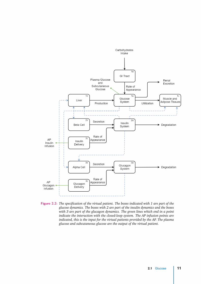
Figure 2.2: The specification of the virtual patient. The boxes indicated with 1 are part of theglucose dynamics. The boxes with 2 are part of the insulin dynamics and the boxeswith 3 are part of the glucagon dynamics. The green lines which end in a pointindicate the interaction with the closed-loop system. The AP infusion points areindicated, this is the input for the virtual patients provided by the AP. The plasmaglucose and subcutaneous glucose are the output of the virtual patient.

2.1 Glucose 11

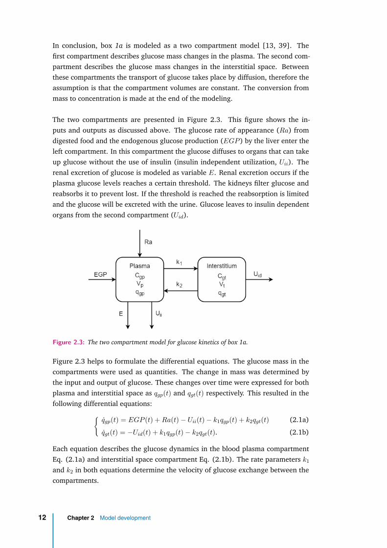
In conclusion, box 1a is modeled as a two compartment model [13, 39]. Thefirst compartment describes glucose mass changes in the plasma. The second com-partment describes the glucose mass changes in the interstitial space. Betweenthese compartments the transport of glucose takes place by diffusion, therefore theassumption is that the compartment volumes are constant. The conversion frommass to concentration is made at the end of the modeling.

The two compartments are presented in Figure 2.3. This figure shows the in-puts and outputs as discussed above. The glucose rate of appearance (Ra) fromdigested food and the endogenous glucose production (EGP ) by the liver enter theleft compartment. In this compartment the glucose diffuses to organs that can takeup glucose without the use of insulin (insulin independent utilization, Uii). Therenal excretion of glucose is modeled as variable E. Renal excretion occurs if theplasma glucose levels reaches a certain threshold. The kidneys filter glucose andreabsorbs it to prevent lost. If the threshold is reached the reabsorption is limitedand the glucose will be excreted with the urine. Glucose leaves to insulin dependentorgans from the second compartment (Uid).

Figure 2.3: The two compartment model for glucose kinetics of box 1a.

Figure 2.3 helps to formulate the differential equations. The glucose mass in thecompartments were used as quantities. The change in mass was determined bythe input and output of glucose. These changes over time were expressed for bothplasma and interstitial space as qgp(t) and qgt(t) respectively. This resulted in thefollowing differential equations:{

qgp(t) = EGP (t) +Ra(t) − Uii(t) − k1qgp(t) + k2qgt(t) (2.1a)

qgt(t) = −Uid(t) + k1qgp(t) − k2qgt(t). (2.1b)

Each equation describes the glucose dynamics in the blood plasma compartmentEq. (2.1a) and interstitial space compartment Eq. (2.1b). The rate parameters k1

and k2 in both equations determine the velocity of glucose exchange between thecompartments.


2.1.1 Endogenous Glucose Production

Box 1b The liver plays an important role in the glucose regulation. At high levelsof glucose plasma it stores glucose and at low levels of plasma glucose it releasesglucose. The liver is both a source and a sink for glucose. After the intake of food,the liver stores the glucose absorbed by the gastrointestinal tract as glycogen. If thereis no intake of carbohydrates, for example during a night sleep, the liver releasesglucose from glycogen. The storage is stimulated by the hormone insulin. Thishormone is released by the pancreas in response to high levels of blood glucose.This storage process is called glycogenesis. The hormone glucagon is released bythe pancreas during low levels of blood glucose. Glucagon stimulates the liverto breakdown the glycogen into glucose. The glucose is subsequently releasedby the liver into the blood plasma. The breakdown process of glycogen is calledglycogenolysis. Figure 2.4 shows the two processes schematically.

Figure 2.4: The left organ is the liver, where the conversion from glucose to glycogen and theother way around occurs. The pancreas is presented on the right. This is the organthat releases the hormones insulin and glucagon. The insulin stimulates glycogenformation and the glucagon stimulates the breakdown of glycogen.

Both glycogenesis and glycogenolysis affect the amount of glucose that passes theliver. The net result of these processes is the hepatic glucose production or EGP.Glycogenesis decreases the EGP, whereas glycogenolysis increases it. EGP is the resultof the glucose regulation by the liver, and depends on the glucose mass in the plasma.The level of glucose determines the secretion of certain hormones by the pancreas.Insulin is secreted during hyperglycemia and stimulates the glycogenesis. Glucagonis secreted during hypoglycemia and stimulates glycogenolysis, subsequently the EGP.Besides these two liver processes, the liver is able to auto-regulate these processes.This auto-regulation is controlled by the glucose mass in the plasma. Hyperglycemiainhibits the rate of glycogenolysis, which is a negative feedback regulation [24,27].

2.1 Glucose 13

Figure 2.5: A compartment overview of the EGP regulation. There are three inputs into theliver which influences the EGP. The plasma insulin concentration (Cip), the plasmaglucagon concentration (Chp) and the plasma glucose mass (qgp). The Cip followsthe route where it passes twice an ODE. The Chp passes once an ODE and the qgp

has a direct effect on the EGP.

Figure 2.5 is an overview of the model for EGP. It shows three inputs for this part ofthe system. Namely, the plasma insulin concentration (Cip(t)), the plasma glucagonconcentration (Chp(t)) and the plasma glucose mass (qgp(t)). Cip(t) follows theroute where it is differentiated twice. The Chp(t) is once differentiated and the qgp(t)has a direct effect on the EGP.

The ordinary differential equations (ODEs) in Figure 2.5 cause a smooth reaction ofthe liver to the changes in hormone concentrations. The reaction is not immediatelyafter a change of concentration. Eqs. (2.2a), (2.2b) and (2.2c) describe the reactionof the liver to the changes in hormone concentrations. An immediate response toa change is physiologically impossible. The insulin concentration in blood plasma(Cip(t)) either increases or decreases. If the insulin increases, it still needs to reachthe site of action, which is in this case the liver. These kinetics are represented bythe ODEs and described by Eq. (2.2a) and Eq. (2.2b). This is in accordance with thestudy of Dalla Man et al. This study describes the insulin action on the liver by twodifferential equations, which seemed to be the best fit to describe the clinical data. Apossible explanation can be that first, the insulin has to diffuse from the portal veinto the interstitial space of the liver tissue. And secondly, it has to bind to certainreceptors located at the cell membranes. The parameter kid is a rate parameterand determine the time between the insulin signal and the insulin action on theliver. The interaction of glucagon with the liver is represented with one differentialequation. The glucagon concentration (Chd(t)) passes one ODE in Figure 2.5 andis described by Eq. (2.2c). This is the hepatic reaction to glucagon. The reactionof the liver is stronger when it crosses the basal value (Chp,b). The parameter khd is


again a rate parameter and describe the time between the glucagon signal and theglucagon action on the liver.

Cx(t) = −kid(Cx(t) − Cip(t)) (2.2a)

Cid(t) = −kid(Cid(t) − Cx(t)) (2.2b)

Chd(t) = −khdChd(t) + khd max[(Chp(t) − Chp,b), 0] (2.2c)

The Cid(t) of Eq. (2.2b) and the Chd(t) in Eq. (2.2c) together with the qgp(t) affectthe EGP (t). This is described by

EGP (t) = EGP0 − kgeqgp(t) − kilCid(t) + khlChd(t) (2.3)

and represents the changes as a result of the liver processes. In Eq. (2.3), EGP0 isthe constant release of EGP. The other terms in Eq. (2.3) are negatively or positivelyaffecting the total EGP as function of time. kgeqgp(t) is the inhibition of glucose onEGP. More specifically, the inhibition of glycogenolysis. The parameter kge representsthe reaction strength of glucose on the liver, or liver glucose effectiveness. kilCid(t)describes the hepatic insulin sensitivity, where the parameter kil is the hepaticresponsivity of insulin. This describes the storage of glucose by the glycogenesisprocess. khlChd(t) in Eq. (2.3) represents the stimulation of EGP by glucagon, whichis the stimulation of the glycogenolysis process. The khl is the hepatic responsivityto glucagon.

Eq. (2.3) describes the changes in the EGP, which is a reflection of the glucoseprocesses in the liver described by Figure 2.4. However, this is not the only glucosemetabolic process that occurs in the liver. The stored glycogen can be exhaustedif glycogen is not supplemented by glycogenesis. This happens when fasting isprolonged. In that situation, the source of available glucose changes, it is constructedfrom the breakdown of proteins. This process is called gluconeogenesis and is autoregulated by the liver instead of by hormones. Hypoglycemia stimulates the rate ofgluconeogenesis when the glycogen reserves are depleted. This process is importantto maintain the blood glucose level. In this model, the gluconeogenesis is notmodeled as it is assumed that the patient in the model does not have prolongedhypoglycemia. Therefore, gluconeogenesis is omitted from the model.

2.1.2 Glucose utilization

Box 1c Glucose is one of the sources for energy in the body. The utilization ofglucose occurs in the cells of the organs via the interstitial space. The glucose absorp-tion into the cells is facilitated by membrane transporter proteins, so called GLUTproteins. This transport is either insulin dependent or insulin independent. The

2.1 Glucose 15

insulin dependent transport occurs in cells where GLUT-4 transporters are present.Insulin works as a key to open the locked cells in order to store the glucose. TheGLUT-4 transporters are mainly found in adipocytes and myocytes. The transportersare not always present on the cell membrane. During euglycemia the GLUT-4 trans-porters are concealed in vesicles inside the cell, about 90% of the transporters areconcealed in this manner [31]. This means that relatively few transporters are activeon the surface of the cell. Hence, the transport of glucose is kept at a low speed.

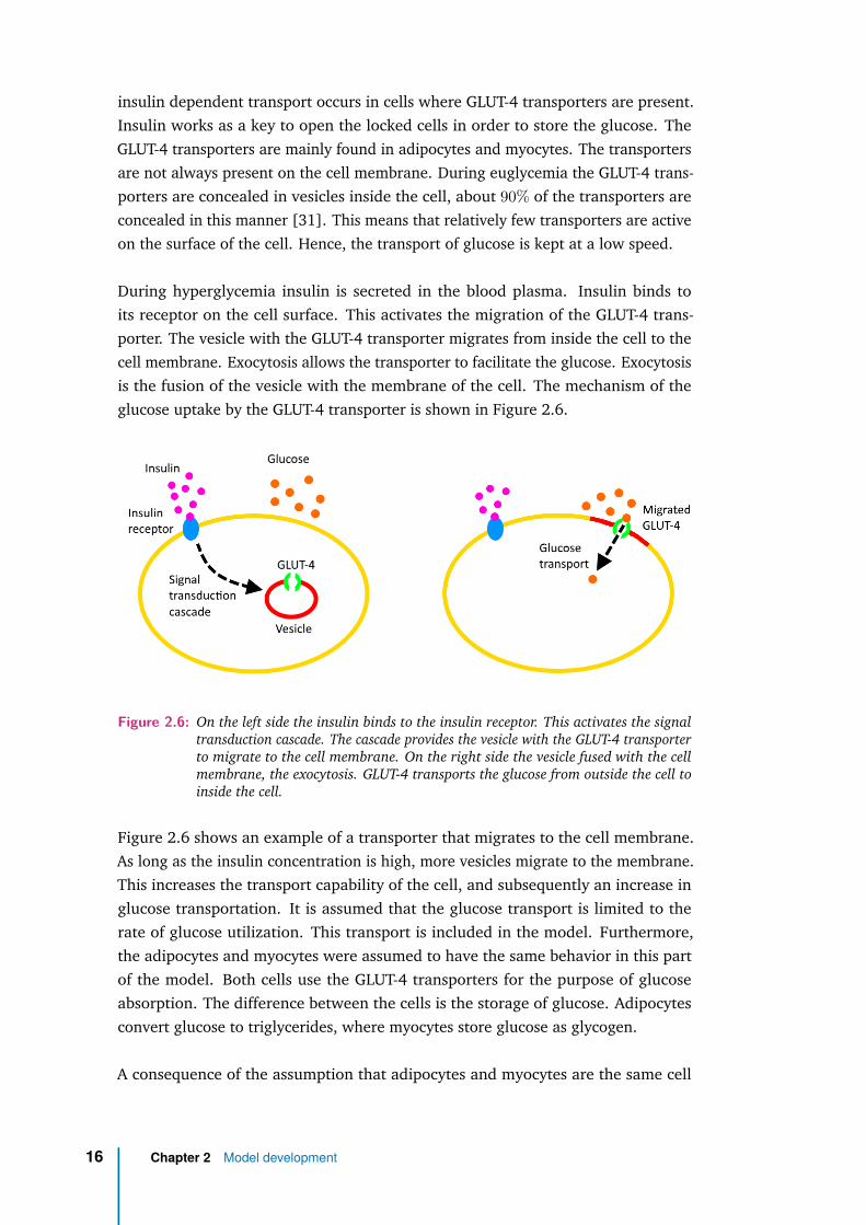
During hyperglycemia insulin is secreted in the blood plasma. Insulin binds toits receptor on the cell surface. This activates the migration of the GLUT-4 trans-porter. The vesicle with the GLUT-4 transporter migrates from inside the cell to thecell membrane. Exocytosis allows the transporter to facilitate the glucose. Exocytosisis the fusion of the vesicle with the membrane of the cell. The mechanism of theglucose uptake by the GLUT-4 transporter is shown in Figure 2.6.

Figure 2.6: On the left side the insulin binds to the insulin receptor. This activates the signaltransduction cascade. The cascade provides the vesicle with the GLUT-4 transporterto migrate to the cell membrane. On the right side the vesicle fused with the cellmembrane, the exocytosis. GLUT-4 transports the glucose from outside the cell toinside the cell.

Figure 2.6 shows an example of a transporter that migrates to the cell membrane.As long as the insulin concentration is high, more vesicles migrate to the membrane.This increases the transport capability of the cell, and subsequently an increase inglucose transportation. It is assumed that the glucose transport is limited to therate of glucose utilization. This transport is included in the model. Furthermore,the adipocytes and myocytes were assumed to have the same behavior in this partof the model. Both cells use the GLUT-4 transporters for the purpose of glucoseabsorption. The difference between the cells is the storage of glucose. Adipocytesconvert glucose to triglycerides, where myocytes store glucose as glycogen.

A consequence of the assumption that adipocytes and myocytes are the same cell


types, is that the effect of physical activity is not present in the model. Physicalactivity augment GLUT-4 transporters in myocytes [23, 29]. The translocation andtranscription increase by frequently exercise. The effect of muscle contraction, whichstimulates migration of GLUT-4 transporters as well, is also ignored in this model.

In conclusion, the facilitated GLUT-4 glucose transport is mediated by insulin. Thisinfluences the rate of glucose absorption by the cells. The Michaelis-Menten equationis commonly used to describe this phenomenon. This equation describes how thevelocity of an enzymatic reaction depends on the substrate concentration. The enzy-matic reaction is the binding of glucose to the GLUT-4 transporter, with glucose asthe substrate. A higher concentration of extracellular glucose increases the transportvelocity. The velocity is also depending on the insulin concentration. The totalglucose utilization is represented by:

U(t) = F + Vm0 + VmciiCii(t)qgt(t)Km0 + qgt(t)

. (2.4)

The fraction in the equation is the Michaelis-Menten representation. Vm0 is the max-imal glucose absorption rate at the maximal level of glucose and Km0 is Michaelis-Menten’s constant at which the glucose utilization is half the Vm0 at the basal levelof insulin. The Michaelis-Menten’s constant expresses the affinity to bind glucose tothe transporter. The lower the value, the higher the affinity for glucose. qgt(t) is theamount of glucose in the interstitial space. F is the glucose utilization of the centralnervous system and the erythrocytes, the red blood cells. The term VmciiCii(t) is theinfluence of insulin on the transport sites, where Cii(t) is the insulin concentrationin the interstitial space. This concentration depends on the insulin concentrationof the blood glucose plasma. Furthermore, the insulin bound to its receptor on thecell membrane is utilized. The insulin concentration in the interstitial space wasdescribed by:

Cii(t) = −pCii(t) + p(Cip(t) − Cip,b). (2.5)

The minus p parameter describes the uptake of insulin by the cells. The plusparameter p represent the diffusion of insulin from the blood to the interstitial space.This diffusion occurs when the plasma insulin concentration (Cip(t)) is higher thanthe basal level (Cip,b).

2.2 Insulin

Box 2a Insulin is a hormone secreted by the pancreas during hyperglycemia. Theinsulin effect is to lower the glucose levels. It facilitates glucose transport in cells,as explained in the previous section 2.1.2. In a healthy person, insulin is secretedin the splenic vein by the pancreatic β-cells during hyperglycemia. This vein drains

2.2 Insulin 17

into the portal venous system of the liver and thereafter in the systemic circulationand body. The anatomical representation is shown in Figure 2.7. The consequenceof the anatomical location of the liver and the pancreas is the insulin extraction bythe liver. Not all the secreted insulin will reach the rest of the body. A part of thesecretion is cleared by the liver and a part stimulates glycogenesis, as discussed inthe section 2.1.1. The liver is responsible for the breakdown and excretion of insulin.The liver regulates the insulin extraction, which results in the regulation of glucose.The insulin regulation by the liver is important to include in the model.

Figure 2.7: The anatomical representation of the organs: liver, pancreas and spleen. Furtherthe veins of the organs are shown. This shows that the splenic vein flows into theportal vein. The portal vein flows to the liver.

The insulin is described by a two compartment model, shown in Figure 2.8. Thecompartments describe the insulin dynamics in the liver and plasma. The firstcompartment represents the liver and the second compartment the plasma. In theliver compartment the insulin extraction is presented by the arrow m3. The arrowm4 is the insulin excretion that occurs in the plasma. This is the insulin extractionby the kidneys.

Figure 2.8: The two compartment model for insulin.


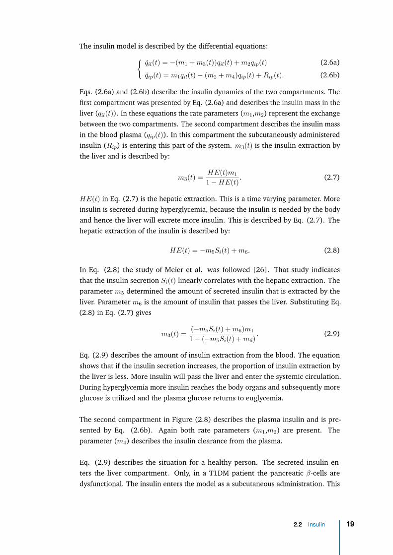
The insulin model is described by the differential equations:{qil(t) = −(m1 +m3(t))qil(t) +m2qip(t) (2.6a)

qip(t) = m1qil(t) − (m2 +m4)qip(t) +Rip(t). (2.6b)

Eqs. (2.6a) and (2.6b) describe the insulin dynamics of the two compartments. Thefirst compartment was presented by Eq. (2.6a) and describes the insulin mass in theliver (qil(t)). In these equations the rate parameters (m1,m2) represent the exchangebetween the two compartments. The second compartment describes the insulin massin the blood plasma (qip(t)). In this compartment the subcutaneously administeredinsulin (Rip) is entering this part of the system. m3(t) is the insulin extraction bythe liver and is described by:

m3(t) = HE(t)m11 −HE(t) . (2.7)

HE(t) in Eq. (2.7) is the hepatic extraction. This is a time varying parameter. Moreinsulin is secreted during hyperglycemia, because the insulin is needed by the bodyand hence the liver will excrete more insulin. This is described by Eq. (2.7). Thehepatic extraction of the insulin is described by:

HE(t) = −m5Si(t) +m6. (2.8)

In Eq. (2.8) the study of Meier et al. was followed [26]. That study indicatesthat the insulin secretion Si(t) linearly correlates with the hepatic extraction. Theparameter m5 determined the amount of secreted insulin that is extracted by theliver. Parameter m6 is the amount of insulin that passes the liver. Substituting Eq.(2.8) in Eq. (2.7) gives

m3(t) = (−m5Si(t) +m6)m11 − (−m5Si(t) +m6) . (2.9)

Eq. (2.9) describes the amount of insulin extraction from the blood. The equationshows that if the insulin secretion increases, the proportion of insulin extraction bythe liver is less. More insulin will pass the liver and enter the systemic circulation.During hyperglycemia more insulin reaches the body organs and subsequently moreglucose is utilized and the plasma glucose returns to euglycemia.

The second compartment in Figure (2.8) describes the plasma insulin and is pre-sented by Eq. (2.6b). Again both rate parameters (m1,m2) are present. Theparameter (m4) describes the insulin clearance from the plasma.

Eq. (2.9) describes the situation for a healthy person. The secreted insulin en-ters the liver compartment. Only, in a T1DM patient the pancreatic β-cells aredysfunctional. The insulin enters the model as a subcutaneous administration. This

2.2 Insulin 19

is explained in the next section 2.2.1. The insulin input appears in the secondcompartment and is shown in Eq. (2.6b) with the term (Rip). Insulin follows adifferent route compared to a healthy person. It enters the blood circulation after thesubcutaneously administration. The physiological first-pass effect is bypassed. Thefirst-pass effect is the effect of the extraction of, in this case, the hormone by the liver.The concentration that enters the liver is lower for the subcutaneous administeredinsulin and, therefore, the liver extraction is lower. This changes Eq. (2.9), becausethe secretion (Si(t)) is not present in T1DM patients. For the model this was changedto the amount of insulin in the plasma (qip(t)). The equation for m3(t) becomesnow:

m3(t) = (−m5qip(t) +m6)m11 − (−m5qip(t) +m6) . (2.10)

2.2.1 Insulin administration

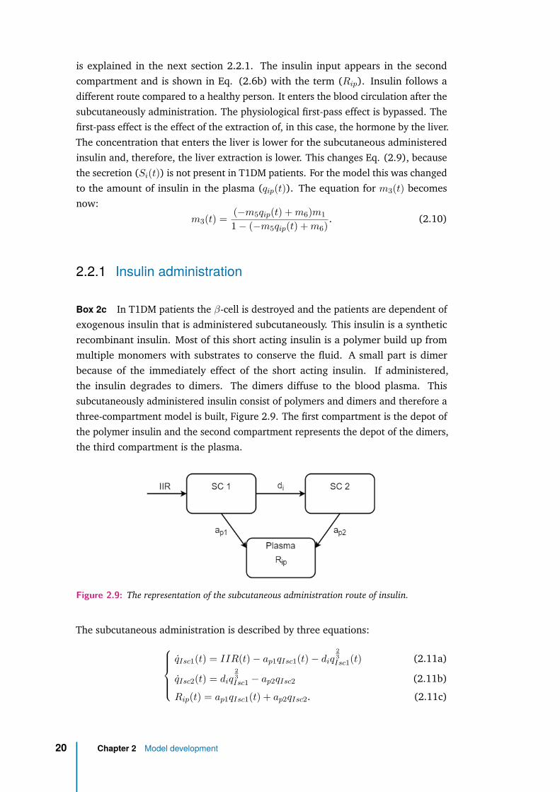
Box 2c In T1DM patients the β-cell is destroyed and the patients are dependent ofexogenous insulin that is administered subcutaneously. This insulin is a syntheticrecombinant insulin. Most of this short acting insulin is a polymer build up frommultiple monomers with substrates to conserve the fluid. A small part is dimerbecause of the immediately effect of the short acting insulin. If administered,the insulin degrades to dimers. The dimers diffuse to the blood plasma. Thissubcutaneously administered insulin consist of polymers and dimers and therefore athree-compartment model is built, Figure 2.9. The first compartment is the depot ofthe polymer insulin and the second compartment represents the depot of the dimers,the third compartment is the plasma.

Figure 2.9: The representation of the subcutaneous administration route of insulin.

The subcutaneous administration is described by three equations:qIsc1(t) = IIR(t) − ap1qIsc1(t) − diq

23Isc1(t) (2.11a)

qIsc2(t) = diq23Isc1 − ap2qIsc2 (2.11b)

Rip(t) = ap1qIsc1(t) + ap2qIsc2. (2.11c)


Eqs. (2.11a) and (2.11b) describe the absorption of the administered insulin. qIsc1(t)in Eq. (2.11a) represents the compartment with the polymers. qIsc2(t) is thecompartment with the dimers represented by Eq. (2.11b). It is assumed that theinjected fluid forms a sphere at the subcutaneous site and that the absorption startsat the surface of the sphere. The decreasing volume of the sphere is describedwith a power of 2

3 . Insulin absorption in the plasma (Rip(t)) is represented by Eq.(2.11c).

2.3 Glucagon

Box 3b Glucagon is secreted by α- cells when the glucose level is low and counter-acts the effect of insulin. Glucagon is secreted into the splenic vein. The splenic veinends up in the portal vein of the liver. The anatomical proximity of the pancreasand liver is advantageous for glucagon’s desired effects. The liver is the main targetorgan for glucagon. Glucagon regulates the hepatic metabolism of glycogen. Itstimulates the liver to release glucose into the circulation by glycogenolysis andgluconeogenesis.

The glucagon concentration in the blood plasma increases by the secretion rateof α-cells. The glucagon concentration decreases by the transport between theplasma and interstitial space. The equilibrium of glucagon is very fast due to itsextremely rapid kinetics [16]. The changes in glucagon plasma concentration isdescribed by:

Chp(t) = −nChp(t) + Sh(t) +Rhp(t). (2.12)

The glucagon removal in the plasma is determined by the rate parameter n. nChp(t)represents the decreasing term of the glucagon concentration in Eq. (2.12). TheSh(t) is the secreted glucagon by the pancreatic α-cells. The glucagon secretion isexplained in the next section 2.3.1. The glucagon concentration is also increasedby the subcutaneously administered glucagon Rhp(t). This is explained in section2.3.2.

2.3.1 Glucagon secretion

Box 3b During hypoglycemia the α-cells sense the low glucose level in bloodplasma. A signal enters the cell through the GLUT-2 transporter, which activates theKAT P channel to actively transport potassium ions. This depolarizes the membranepotential, establishing a less negative potential across the cell membrane. Thisresults in an influx of sodium ions and influx of calcium ions. The increase of calciumactivates the glucagon release. This process is shown in Figure 2.10. The glucagon

2.3 Glucagon 21

secretion depends on the depolarization of the α-cell membrane. In the opposite case,the hyperpolarization of the cell membrane reduces the glucagon release. For higherglucose concentration there is no signal given by the GLUT-2 transporter, whichprevents the KAT P channel to excrete potassium. The intracellular concentrationbecomes more negative, reducing the glucagon release.

Figure 2.10: The action potential of the alpha cell and secretion pathway of glucagon. Duringlow levels of glucose the alpha cell senses this and allows KAT P to secrete K+,this depolarizes the cell. Na+ enters the cell, followed by Ca2+. The calciumactivates the secretion of glucagon. The release of glucagon happens pulsatile.

Glucagon secretion follows an episodic secretion. This pattern is described by twophases, the static and dynamic phase. The two phase secretion is represented by theequations:

Sh,static(t) = −ρ[Sh,static(t) − max[σ(h− Cgp(t)) + Sh,b, 0)] (2.13a)

Sh,dynamic(t) = δmax[−Cgp(t), 0] (2.13b)

Sh(t) = Sh,static(t) + Sh,dynamic(t). (2.13c)

If the glucose concentration gets below a certain glucose level, glucagon is secreted.This moment is indicated in Eq. (2.13a) by [h − Cgp(t)], where h is the threshold.This applies for the static part. Parameter ρ is the rate parameter for the staticrelease. σ is the α- cell responsivity to the glucose level in the plasma. The static partwas limited by the max function. If the condition σ[h− Cgp(t)] + Sh,b is higher thanzero, the condition contributes to the secretion, otherwise this part of the equationis zero. The Sh,b is the basal glucagon secretion. The dynamic part described by Eq.(2.13b) depends on the decreasing rate of the plasma glucose concentration. δ is therate parameter for the dynamic part. Again, this equation was limited by the maxfunction. The total secretion is the addition of the static (Sh,static(t)) and dynamicsecretion (Sh,dynamic(t)).


2.3.2 Glucagon administration

Box 3c The subcutaneous administration of glucagon is assumed to follow thesame pathway as the subcutaneous administration of insulin. The study of Lv etal. indicates that a three-compartment model is the best way to describe glucagondynamics of the subcutaneous route. The compartments are represented in Figure2.11. Again, the assumption is made that the fluid forms a sphere once administered.This is in contrast to the study of Lv et al.

Figure 2.11: Representation of the subcutaneous administration route of glucagon.

The subcutaneous administration of glucagon is described by three equations:qHsc1(t) = HIR(t) − bp1qHsc1(t) − dhq

23Hsc1(t) (2.14a)

qHsc2(t) = dhq23Hsc1 − bp2qHsc2 (2.14b)

Rhp(t) = bp1qHsc1(t). (2.14c)

Eqs. (2.14a) and (2.14b) describe the absorption of the subcutaneously administeredglucagon. qHsc1(t) represents the changes of administered glucagon in the firstcompartment and qHsc2(t) the changes in the second compartment. The decreasein volume of glucagon is also described with a power of 2

3 . Glucagon absorption inthe blood plasma (Rhp(t)) is represented by Eq. (2.14c). This is slightly differentcompared to insulin. The glucagon absorption in the plasma is only from the secondcompartment. In contrast to the insulin, where the absorption is from the first andthe second compartment. The outflow from the first compartment is lost.

2.4 Model

A virtual patient is modeled by the submodels indicated in Figure 2.2. Thesesubmodels are explained in the previous sections, except for the GI tract. Thisis discussed in section 5.1. The submodels describe the three main physiologicalsubsystem of the glucose regulation, the glucose, insulin and glucagon. The glucose

2.4 Model 23

subsystem consists of 4 parts and the first 3 are modeled during this study by 8mathematical equations. The insulin subsystem is divided into 3 parts and 2 aremodeled in this study, because the β-cell part is assumed to be zero. 6 mathematicalequation are used to describe the insulin subsystem. The glucagon subsystemconsists of 3 parts and are all modeled in this study by 7 mathematical equation.In summary, the total model is divided into 10 parts as Figure 2.2 shows and existsof 14 differential equations and 7 mathematical equations. The model consistsof 35 parameters that need to be estimated and calculates 28 output values. Theparameters and outputs are listed in Table 2.1. The abbreviations used in theequations are explained by the quantity and the unity.


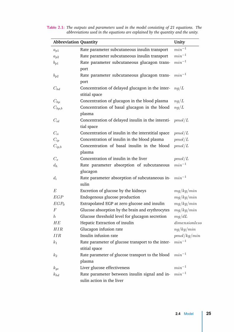
Table 2.1: The outputs and parameters used in the model consisting of 21 equations. Theabbreviations used in the equations are explained by the quantity and the unity.

Abbreviation Quantity Unity

ap1 Rate parameter subcutaneous insulin transport min−1

ap2 Rate parameter subcutaneous insulin transport min−1

bp1 Rate parameter subcutaneous glucagon trans-port

min−1

bp2 Rate parameter subcutaneous glucagon trans-port

min−1

Chd Concentration of delayed glucagon in the inter-stitial space

ng/L

Chp Concentration of glucagon in the blood plasma ng/L

Chp,b Concentration of basal glucagon in the bloodplasma

ng/L

Cid Concentration of delayed insulin in the intersti-tial space

pmol/L

Cii Concentration of insulin in the interstitial space pmol/L

Cip Concentration of insulin in the blood plasma pmol/L

Cip,b Concentration of basal insulin in the bloodplasma

pmol/L

Cx Concentration of insulin in the liver pmol/L

dh Rate parameter absorption of subcutaneousglucagon

min−1

di Rate parameter absorption of subcutaneous in-sulin

min−1

E Excretion of glucose by the kidneys mg/kg/min

EGP Endogenous glucose production mg/kg/min

EGP0 Extrapolated EGP at zero glucose and insulin mg/kg/min

F Glucose absorption by the brain and erythrocytes mg/kg/min

h Glucose threshold level for glucagon secretion mg/dL

HE Hepatic Extraction of insulin dimensionless

HIR Glucagon infusion rate ng/kg/min

IIR Insulin infusion rate pmol/kg/min

k1 Rate parameter of glucose transport to the inter-stitial space

min−1

k2 Rate parameter of glucose transport to the bloodplasma

min−1

kge Liver glucose effectiveness min−1

khd Rate parameter between insulin signal and in-sulin action in the liver

min−1

2.4 Model 25

Table2.1 – continued from previous page


khl Glucagon action on the liver mg/kg/min

per ng/L

kid Delay parameter between insulin signal and in-sulin action

min−1

kil Insulin action on the liver mg/kg/min

per pmol/L

Km0 Michaelis-Menten constant for GLUT-4 mg/kg

m1 Rate parameter of insulin transport to the bloodplasma

min−1

m2 Rate parameter of insulin transport to the inter-stitial space

min−1

m3 Rate parameter of insulin transport from the liver min−1

m4 Rate parameter of insulin from the blood plasma min−1

m5 Rate parameter of secreted insulin to the bloodplasma

min−1

m6 Rate parameter of hepatic insulin extraction min−1

n Rate parameter of glucagon from the bloodplasma

min−1

p Rate parameter of insulin to the interstitial space min−1

qgp Mass of glucose in the blood plasma mg/kg

qgt Mass of glucose in the interstitial space mg/kg

qHsc1 Mass of glucagon in the subcutaneous space ng/kg

qHsc2 Mass of glucagon in the subcutaneous space ng/kg

qil Mass of insulin in the liver pmol/kg

qip Mass of insulin in the blood plasma pmol/kg

qIsc1 Mass of insulin in the subcutaneous space pmol/kg

qIsc2 Mass of insulin in the subcutaneous space pmol/kg

Ra Rate of appearance of glucose in the bloodplasma after carbohydrate intake

mg/kg/min

Rhp Rate of appearance of glucagon in the bloodplasma

ng/kg/min

Rip Rate of appearance of insulin in the blood plasma pmol/kg/min

Sh Secretion of glucagon by the pancreatic alphacells

ng/kg/min

Sh,dynamic Secretion of dynamic phase of glucagon by thepancreatic alpha cells

ng/kg/min

Sh,static Secretion of static phase of glucagon by the pan-creatic alpha cells

ng/kg/min




Sh,b Basal glucagon secretion by the pancreatic alphacells

ng/kg/min

Si Secretion of insulin by the pancreatic beta cells pmol/kg/min

U Total utilization of glucose mg/kg/min

Uid Insulin dependent utilization of glucose mg/kg/min

Uii Insulin independent utilization of glucose mg/kg/min

Vm0 Maximal velocity of glucose mg/kg/min

Vmcii Maximal velocity of glucose transport dependenton insulin

mg/kg/min

per pmol/L

δ Sensitivity parameter of the alpha cell to glucose ng/L per

mg/dL

ρ Rate parameter of the glucagon secretion intothe blood plasma

min−1

σ Alpha cell responsivity to glucose level ng/L/min

2.4 Model 27

3Simulation

In chapter 2 the mathematical description of the model is described. The model isdesigned to simulate T1DM patients suitable for testing the AP’s algorithm. It repre-sents the glucose regulation system by describing the glucose, insulin and glucagondynamics. These are the three subsystems and their interaction are modeled.

As mentioned before, the model reacts on the administered hormones receivedfrom the AP as an input. The model provides the simulated glucose values. Theglucose values are the output of the model. These values are shown in a graph.Furthermore, it is interesting to monitor additional parameters to serve as valuablefeedback for the researcher. Plasma insulin and glucagon concentration affect theEGP and glucose utilization, all of which influence the glucose concentration in theblood plasma. These four additional parameters are also plotted in graphs.

In this chapter an example is given of simulation result. Figure 3.1 shows theoutputs of the simulation. For the simulation the values presented in the study ofDalla Man et al. are used. The parameter values for a healthy person are usedbecause of the missing values of T1DM patients. A signal is reconstructed to simulatethe glucose appearance in the blood plasma. This is the effect of the intake of amixed meal containing 78 g of glucose [13]. The model does not simulate the β-cell.Therefore, the insulin is simulated similar to the MDI therapy and thus provided by1 subcutaneously insulin injection. This administration is also modeled as a shortimpulse to the system by 100 units of insulin an equivalent to 3.5 mg insulin.

Three simulations are performed. The first simulation is an example of a glu-cose input by a meal. The insulin is subcutaneous injected and at the same timethe intake of carbohydrates is started. This is normal procedure for T1DM patients.When a T1DM patient eats, he or she should count the amount of carbohydratesbefore the meal. Patients have to inject a calculated amount of insulin correspondingto the amount of carbohydrates. Secondly, a simulation is performed of a patientwho injected the same calculated amount of insulin, but administered it 30 minutesafter the start of the glucose appearance. This can occur if a patient forgets to injectthe insulin in time. The third simulation represents an injection of insulin, whilethe patient did not eat in time and eats less carbohydrates than anticipated. Thepatient started eating 30 minutes after the injected insulin and eat 39 g of glucose,

29

which is half the meal. Therefore, the amount of administrated insulin is higher thanrequired. This happens when something interrupts diner time and the patient eatless than expected. These three situation are represented in Figure 3.1. Where theblue line is simulation 1, the red dashed line is simulation 2 and the green dottedline is simulation 3.

Figure 3.1b is the input to the system, the glucose appearance in the blood plasmafrom a digested meal. It shows an impulse response that slowly decreases overthe hours. Figure 3.1c shows the hepatic EGP. Figure 3.1d represents the insulinconcentration in the blood plasma as a result of the subcutaneously administeredinsulin. Figure 3.1e presents the total utilization of glucose. Figure 3.1f shows theplasma glucagon. The glucagon is secreted by the α-cells in reaction to low plasmaglucose levels. Glucagon is not subcutaneously administered in these simulations.The EGP and utilization influence the plasma glucose level and are affected by thehormones insulin and glucagon. Furthermore, each graph of Figure 3.1 shows the 3simulated situations.

Looking at the first simulation. Figure 3.1a shows a peak in glucose concentra-tion. The glucose plasma concentration returns to its steady state with a smallfluctuation after 2 hours. A small increase is seen from 2 to 4 hours, after which itincreases again. While glucose is still available up to 6 hours after eating, see Figure3.1b. The slightly elevated glucose concentration after the main peak starts at thesame time as the EGP increases. The plasma insulin reaches a peak within an hourand disappears within 2 hours. Only, the effect of insulin is longer present. This isseen in Figure 3.1e. The peak of the glucose utilization starts at the same time asthe plasma concentration peak of insulin. After 3 hours the utilization is back to thebasal state, which is longer than the present of insulin in the plasma. As soon asthe glucose concentration decreases, the plasma glucagon increases. This is seen inFigure 3.1f, where at 1 hour the increase in plasma glucagon is shown.

Next simulation 1 and 2 are compared with each other. In Figure 3.1 these sit-uations are represented by the blue and red curves, respectively. The red curvein Figure 3.1a shows what happens with the plasma glucose, when the insulininjection is administered after a meal. The glucose concentration increases morethan for simulation 1 and reaches a higher maximum. The administered insulin afterthe meal results in a later utilization peak. At the time the insulin concentrationincreases in the blood plasma and utilization increases at the same time as Figure3.1e shows. Noticeable is that the utilization peak reaches a higher level for thesame amount of insulin. This higher level is caused by the higher level of glucoseconcentration. Figure 3.1c shows that the suppression of EGP differs for the lateradministered insulin. The suppression is immediately present, this is caused by theincrease of glucose. The higher glucose peak also decreases faster, this results in a

30 Chapter 3 Simulation

stronger glucagon reaction. Figure 3.1f shows this stronger increase in the glucagonconcentration.

Finally the third situation is simulated. This is the situation where a smaller mealis taken at a later time. Figure 3.1a shows a decrease of glucose. This decrease isthe effect of the administered insulin without intake of carbohydrates. The insulinin Figure 3.1d follows the same curve as in the first simulation. The reaction inglucose utilization starts at the same moment. Only, this time the utilization does notreach a level as high as for the first simulation. This is expected, since the glucoseappearance is not present yet. Due to a decrease in glucose, the plasma glucagonincreases. This effects the EGP, as is seen in Figure 3.1c. Contrary to simulations 1and 2, the EGP increases. The higher EGP and glucose appearance both increase theglucose plasma concentration.

31

(a) Plasma glucose (b) Rate of appearance of glucose

(c) Endogenous glucose production (d) Plasma insulin

(e) Utilization of glucose (f) Plasma glucagon

Figure 3.1: Output of the three simulations. The first simulation shows the insulin injectedbefore eating, after which the glucose appearance started. The second simulationis the situation, where the insulin is injected after eating the meal. The thirdsimulation, the meal is delayed. The insulin is injected and the meal appearsminutes later. As input signal the rate of appearance is given. The input is shownin the right upper plane.

32 Chapter 3 Simulation

4Parameter estimation

In Table 2.1, there are 35 parameters that need to be estimated. The other 28 areoutput values and are calculated by the model. This is a large number of parametersand can’t be estimated at once all together. Estimation of the glucagon subsystemwas approached first. The glucagon subsystem comprises of the subcutaneous ad-ministration of the glucagon, the glucagon kinetics in the plasma and the glucagonsecretion by the α-cells. With the available clinical data provided by the study ofBlauw et al. the glucagon secretion by the α-cells cannot be estimated [3]. Theglucagon estimation is done for the subcutaneous administration and the plasmaglucagon.

The clinical data considered 6 T1DM patients, who each visited a clinical researchcentre three times. Patients underwent a glucose clamp procedure to establish acertain blood glucose level during these visits. When the required blood glucoselevel was reached, a glucagon dose was administered. A blood sample was takento analyze the glucagon pharmacokinetics every 10 minutes. 4 tests per visit wereperformed. The study schedule is shown in Table 4.1. For every subject there are 12measurements.

9 data points were collected during each measurement. For one measurementthe data points are depicted in red in Figure 4.1. The y-values are the glucagonconcentration in the blood and were shifted, so that the y0 starts at 0. This meansy0 = 60.8 is substracted from every y-value At t = 0 the glucagon was subcutaneouslyadministered and data points were collected every 10 minutes.

Table 4.1: The schedule for the glucagon data collection in the study [3].

Visit Bloodglu-coselevel(mmol/L)

Glucagondose(mg)

Bloodglu-coselevel(mmol/L)

Glucagondose(mg)


Glucagondose(mg)


Glucagondose(mg)

A 8 0.11 6 0.11 4 0.11 2.8 1.0B 8 0.22 6 0.22 4 0.22 2.8 0.66C 8 0.44 6 0.44 4 0.44 2.8 0.33

33

Figure 4.1: The scaled glucagon data of one measurement and the new calculated y from theparameter estimation.

These three differential equation were used for the parameter estimation:Chp(t) = −nChp(t) + Sh(t) + bp1qHsc1(t) (4.1a)

qHsc1(t) = HIR(t) − bp1qHsc1(t) − dhq23Hsc1(t) (4.1b)

qHsc2(t) = dhq23Hsc1 − bp2qHsc2. (4.1c)

These are Eqs. (2.14a) and (2.14b) as mentioned in the section 2.3.2. The Eq.(2.14c) is substituted in to Eq. (2.12), which gives Eq. (4.1a).

Due to the power of 23 , the equations are non-linear. The equations were linearized

by the Taylor polynomial method in the equilibrium point to estimate the parameters(bp1, bp2, dh, n) in Eqs. (4.1a), (4.1b) and (4.1c). This equilibrium point is found bysetting the input to 0, when there is no glucagon subcutaneously administered. Theequilibrium point is represented in Eq. (4.2).

Chp,eq = ( dh

−bp1)3 (4.2)

With the Eqs. (4.1a), (4.1b) and (4.1c) the following transfer function from theinput HIR to the output Chp was found:

H = 2bp2d4h

b3p1(bp2 + s)(n+ s)(bp1 + 3s)

. (4.3)

With this transfer function the parameters can be estimated using the ARX methodin Matlab. This function uses the least squares method. The transfer function showsthat the A-polynomial, the denominator in the fraction, is of the third order. The

34 Chapter 4 Parameter estimation

B-polynomial, the numerator of the fraction, is a zero order polynomial. The ARXmathematical representation is:

yk = B(z)A(z)uk + 1

A(z)ek. (4.4)

Furthermore, there is a delay in the input-output relation. This can be seen in thedata of Figure 4.1. The input starts at t0 and the first output is seen at t1. Thisaccounts for a delay of one sample time and limits the possibilities of the estimation.As presented in Figure 4.1, 2 data points are added in the past. The estimation withARX is an estimation in the z-transform. The ARX needs data points in the past, dueto the order of the A-polynomial. These extra data points are assumed to be zero,because the system reacts after the given input. For the z-transform the followingequations present the polynomial of the ARX in this case:{

A(z) = 1 + a1z−1 + a2z

−2 + a3z−3 (4.5a)

B(z) = b0. (4.5b)

The estimation is performed in Matlab and is presented in Figure 4.1. The bluedashed line is the new y-values for the estimated parameters and follows the datapoints. This is an example of one measurement in a single subject. There are 12data sets for each patient where the conditions vary. As indicated in Table 4.1 theblood glucose levels and the glucagon dosages are different for every measurement.The estimation as described above were done for every data set. These differentconditions need to indicate if the parameters are dependent on the blood glucosevalue or the glucagon dosages. The three A-polynomial parameter values (a1, a2, a3)with their standard deviation are plotted in Figure 4.2. At this point the parameterof the B-polynomial is leaved out of consideration. There are 12 measurementsshown in Figure 4.2 all from 1 subject. The parameters show a varied pattern. Thisindicates that the conditions of the measurements influence the model parameters.The ideal pattern is a horizontal line, this indicates than that the blood glucose andglucagon dosage does not influence the glucagon pharmacokinetics in 1 patient.

Looking at Figure 4.1 the estimation seems a good representation of the data.Only, the parameters values that are estimated to describe the results are complexnumbers. This is inconsistent with the model equations. The expectation is that thehuman physiology is described by real numbers instead of complex numbers. Theresults with complex numbers are a structurally estimation error and appears in allmeasurements and in all subject.

35

Figure 4.2: Parameters of A-polynomial (a1, a2, a3) with the standard deviation for 1 subjectthe 12 measurements are present.

36 Chapter 4 Parameter estimation

5Discussion

This study provides insight in the human glucose regulation by designing a simulationmodel to test the algorithm of the AP of Inreda Diabetic BV. A simulation model wasdesigned to test the algorithm of the AP of Inreda Diabetic BV. This model representsthe glucose regulation system of T1DM patients. This representation is achieved bymodeling three main physiological subsystems, the glucose, insulin and glucagondynamics. For all the subsystems the physiological processes are explained. Inaddition, a major part of this study was obtaining the mathematical representationof the physiology. First simulation results proved that the model can simulate theglucose regulation, albeit with parameters from the literature.

5.1 Glucose

The glucose subsystem is described in several parts, namely the glucose regulation bythe liver, the blood plasma glucose, the glucose utilization and absorption of glucose.The liver plays an important role in the glucose regulation and when diabetes pro-gresses, the regulation by the liver changes [24]. This crucial role justifies to modelthe liver as a separate part. The EGP is influenced by glucose and two hormones,insulin and glucagon. The effects of the two hormones on the EGP are describedby ODEs. Insulin’s effect is described by two ODEs and the effect of glucagon isdescribed by one ODE. In Figure 3.1c, the inhibition of EGP by glucose seems thestrongest regulator. When the insulin is administered after the appearance of glu-cose, simulation 2, hardly any difference is seen in the decrease of EGP betweensimulation 1 and simulation 2. This is in contrast with the study of Dalla Man et al.[13]. Besides this, the stimulating effect of glucagon on EGP seems lower than theinhibiting effect of glucose and insulin together. The EGP is increased by glucagon,but this effect is not as strong as the decrease of EGP by glucose. This indicates thatthe implementation of EGP in the model might need adjustments to balance theinfluences on EGP of glucose and both hormones.

The glucose utilization is represented by the well-known Michaelis-Menten equation.This standard equation described the glucose transport into a cell by the GLUT-4transporters. Figure 3.1e shows a good response to the insulin. It responses mainly toinsulin and only slightly to glucose. The glucose utilization model could be expanded

37

by including physical activity. In section 2.1.2 the muscles and adipose tissues areassumed the same and the effect of physical activity was omitted. Nevertheless, phys-ical activity has a major effect on the glucose utilization [5, 14, 30] and should beimplemented in this model. The adipose tissue and muscles should be modeled sep-arately. The GLUT-4 transporters in myocytes migrate under the influence of insulinand by contracting the muscles [29]. The response to this contraction depends onthe intensity level of the physical activity. The GLUT-4 migration by the contractingmuscles influences the Michaelis-Menten curve and should be implemented in themodel. The process of gluconeogenesis in the liver is important during prolongedfasting and it becomes beneficial during physical activity. The glycogen source israpidly exhausted by the energy demand of the muscles. If the physical activity isimplemented in the model the contribution of gluconeogenesis has to be investigated.

The part that was not described in the chapter 2 is the GI tract. This must bemodeled to simulate the glucose regulation in T1DM patient for different meals.Modeling of the GI tract can be done using compartments, i.e. considering theliquid and solid phase and the content of the meal. These influence the gastricemptying and therefore the glucose absorption in the blood plasma. This method isimplemented in the study of Dalla Man et al. [13]. Another possible method is thesimulation of glucose absorption from the food according to the glycemic index. Theglycemic index ranks the carbohydrates in food by the extent to which they raiseblood glucose levels after eating on a scale from 0 to 100 [18]. Food with a higherpeak in postprandial blood glucose and a greater elevated blood glucose level, twohours after the intake, has a high glycemic index. These carbohydrates are rapidlydigested and absorbed, hence result in fluctuating blood glucose levels. Food with alow glycemic index is slowly digested and absorbed, resulting in a lower peak anda steady rise of the blood plasma. An attempt was made to simulate the glucoseabsorption using the glycemic index. However, connecting the GI tract to the glucosesubsystem proved to be difficult. The meal volume settings and the meal glycemicindex seems to be inaccurate. The rate of glucose appearance in the blood plasmawas mainly affected by the meal volume and less by the glycemic index of the meal.The expectation is that the glycemic index mainly determines the glucose appearancein the blood plasma. Therefore, changing the parameter settings could be a solution.Otherwise the mathematical submodel of the GI tract should be reconsidered.

5.2 Insulin

At this moment, the AP is designed for and tested with T1DM patients, however theAP might also treat type 2 diabetes mellitus (T2DM) patients in the future. At thispoint the model does not contain β-cells, because the pancreatic insulin secretion

38 Chapter 5 Discussion

is assumed to be zero for T1DM patients. Ideally, the AP will be tested with thesimulation model, before the clinical trials with T2DM. β-cell must be modeled toperform this simulation. It is important to consider the two phasic secretion ofinsulin by β-cells [4, 36]. The first phase is a fast insulin release and the secondphase a slower insulin release. Although the secretion phases are impaired in T2DMpatients [26], both phases still need to be modeled. The plasma insulin in T2DMpatients still shows the two phased secretion. The liver also contributes to the insulinregulation [6, 35]. The anatomical location of the liver and the pancreas results inthe insulin extraction by the liver. Not all the secreted insulin will reach the rest ofthe body. This regulation by the liver is already implemented in the model, whichmakes the extension of β-cell a small step.

The subcutaneous route of insulin is implemented with a spherical release of theadministered insulin. The study of Lv et al. concludes that the subcutaneous admin-istration route shows a delayed clearance of insulin and a biphasic appearance in theblood plasma [25]. The delayed clearance is partly met by the spherical release inthe model, due to the slower absorption. Simulation with a spherical release showsthat the administered insulin is longer present in the blood plasma. The biphasicappearance is not simulated and can be implemented by a fourth order polynomial.This makes the model more complex and affects the parameter estimation for thispart of the model. The data has to be sufficiently rich, e.g. contain the biphasicappearance to estimate the unknown parameters. The available clinical data cannotdescribe the unknown parameters [7]. The spherical release is the best solution tothis point.

Figure 3.1d shows the rise in the plasma insulin and a return back to zero af-ter 1.5 hours. This is a quickly return compared to other studies [12, 25] and seemsunrealistic. Insulin used in the AP has a duration of effectiveness between 2 and 5hours. The simulated insulin in the plasma is cleared in 2 hours and is faster thanexpected. Next, the simulation used 100 units of administered insulin. This is anunlikely amount of insulin. The parameters values found in the literature can causethis effect. Using other parameter settings might slow the insulin clearance.

5.3 Glucagon

As mentioned in chapter 1, the glucagon kinetics and dynamics are important tosimulate in the model. The review of Wilinska et al. and the review of Colmegna et al.indicate that there was no existing model that simulates the glucagon subsystem [11,38]. After the published reviews, the UVA/Padova model is expanded by includingthe glucagon kinetics and dynamics. Since the extension of this model is based on

5.3 Glucagon 39

non-published assumptions, there is uncertainty about its accuracy. In this study thedesigned model for testing the AP also considers the glucagon part for the simulation.Compared to the UVA/Padova model the subcutaneous administration for glucagonis added in the same way as the subcutaneous administration for insulin in thisstudy. In addition, the glucagon secretion by the α-cells are differently modeled.This is a second difference to the UVA/Padova model. The results show the glucagonsecretion, which consists of the static and dynamic secretion as explained in section2.3.1. The static part reacts on the plasma glucose concentration and the dynamicpart to the change of plasma glucose concentration. This is in consistence with theinsulin secretion modeled in other studies [4, 13, 26, 36] and the base for the α-cellsecretion. Figure 3.1f indicates that the glucagon secretion is primarily regulatedby the dynamic part. This is shown in the last part of the curve after 4 hours

where the secretion increases. This increase is the result of the secretion stimulatedby the dynamic part of the glucagon secretion. The dynamic part reacts on thechange of the glucose level. This indicates that the dynamic part of the secretionreacts on the fluctuations in the blood glucose, even if there is hyperglycaemia.The glucagon secretion in this model should be reconsidered. Furthermore, theinsulin level inhibits the glucagon secretion. This negative feedback is not coveredby mathematical representation.

The effect of glucagon on EGP is shown in Figure 3.1c in the third simulation. Itshows an increase in EGP as reaction to the increased glucagon secretion. Only,the result of the increased EGP on the blood plasma glucose is not clearly seen inFigure 3.1a. The increase of the glucose concentration in the blood plasma seems tobe a result of the glucose appearance after the intake of carbohydrates instead ofan increase of EGP. The expectation was that the EGP is able to drive the glucoselevel back to the steady state. A possible explanation for the weak reaction is theuse of the parameters values for this simulation. The parameters are based on theliterature. The parameters for the glucagon part are provided by another study thanthe parameters of the other model parts. This can explain the weak reaction to theglucagon concentration, because the parameters are not estimated based on thesame clinical data.

5.4 Parameters

At this moment the model consists of 35 parameters, which may increase as themodel changes. Ideally these parameters all need to be estimated. However, thisis difficult due to the poorly available clinical data. Therefore, some parametersare searched for in the available literature. Notice that these are mostly the meanvalues for a parameter. To provide the inter and the possible intra patient differences,

40 Chapter 5 Discussion

using the mean values for the parameters is unreliable. A first step was made toestimate the parameters of the model. The estimation started with the glucagonpart. This choice was made due to the available clinical data. This study usedthe ARX method to estimate the parameters, which uses the linear least squaremethod. Surprisingly, this method provides complex numbers, which was not to beexpected. Physiologically, the parameter values are real numbers. According to thefit, represented in Figure 4.2, it seemed a good method. The first attempt indicatesthat the parameter estimations are not straightforward and that further work shouldfocus on the estimation of the parameters.

A possibility can be to force the ARX method to return real values. Another pos-sibility is reconsidering the method to estimate the parameters. Alternatively, theOutput-Error method was tried, this is another method to estimate the parameters.This method does not consider the disturbance to the system. It assumes that thedisturbance is a white noise signal. The Output-Error method gave similar valuesfor the estimated parameters as the ARX model gave. And the fit does not show agreat difference to the ARX fit. The ARX method was chosen, because it consideredthe disturbance term 1

A(z)ek. The disturbance is important to account for, becausebecause in the model, different assumptions were made and the collection of thedata is expected to cause disturbance in the model. This disturbance is also part ofthe estimation.

It is a challenge to acquire the necessary clinical data. In general, the data hasto be rich enough to contain the unknown parameters for the estimation. The dataneed to be sufficiently rich for the model considered. The clinical data might beenriched by measuring additional variables. Finding clinical data for the submodelsas the liver and utilization and the secretion of both hormones will be difficult. Forexample, to estimate the EGP parameters it is ideally required to known the plasmaglucose in the portal vein and the plasma glucose in the hepatic vein. In this waythe effect of the EGP can be estimated by the change of the glucose level.

5.4 Parameters 41

6Conclusion

This study provides a substantial basis for the in silico testing of the AP developed byInreda Diabetic BV. The model provides more insight in the human glucose regulationand can be helpful in the development and testing processes for the AP. The modelrepresents the glucose regulation system in T1DM patients. The model consist of10 submodels, that describe the three main physiological subsystems, the glucose,insulin and glucagon processes. These processes are described by fifteen differentialequations and the seven mathematical equations. In total there are 35 parametersand 28 outputs. First simulation results proved that the model can simulate theglucose regulation. Therefore, this model is a valuable tool for preclinical testing ofthe AP.

43

Bibliography

[1]B. W. Bequette. “A critical assessment of algorithms and challenges in the developmentof a closed-loop artificial pancreas”. In: Diabetes technology & therapeutics 7.1 (2005),pp. 28–47 (cit. on p. 5).

[2]H. Blauw, A.C. van Bon, R Koops, and J.H. DeVries. “Performance and sagety of anintegrated bihormonal artificial pancreas for fully automated glucose control at home”.In: Diabetes, Obesity and Metabolism 18.March (2012), pp. 671–677 (cit. on p. 3).

[3]H. Blauw, I. Wendl, J. H. Devries, T. Heise, and T. Jax. “Pharmacokinetics and pharma-codynamics of various glucagon dosages at different blood glucose levels”. In: Diabetes,Obesity and Metabolism 18.1 (2016), pp. 34–39 (cit. on pp. 6, 33).

[4]E. Breda, M. K. Cavaghan, G. Toffolo, K. S. Polonsky, and C. Cobelli. “Oral glucosetolerence test minimal model indexes of beta-cell function and insulin sensitivity”. In:Diabetes 50.1 (2001), pp. 150–158 (cit. on pp. 39, 40).

[5]M. D. Breton. “Physical Activity: the major unaccounted impediment to closed loopcontrol”. In: Journal of Diabetes Science and Technology 2.1 (2008), pp. 169–174 (cit. onp. 38).

[6]M. Campioni, G. Toffolo, R. Basu, R. A. Rizza, and C. Cobelli. “Minimal model assess-ment of hepatic insulin extraction during an oral test from standard insulin kineticparameters.” In: American Journal of Physiology Endocrinology and Metabolism 297(2009), E941–E948 (cit. on p. 39).

[7]E. Carson and C. Cobelli. Modelling methodology for physiology and medicine. 2001.arXiv: arXiv:1011.1669v3 (cit. on pp. 3, 39).

[8]L. J. Chassin, M. E. Wilinska, and R. Hovorka. “Evaluation of glucose controllers invirtual environment: methodology and sample application.” In: Artificial intelligence inmedicine 32.3 (2004), pp. 171–81 (cit. on p. 4).

[9]M. Cnop, N. Welsh, J. Jonas, A. Jo, and S. Lenzen. “Mechanisms of pancreatic beta-celldeath in Type 1 and Type 2 diabetes”. In: Diabetes 54.2 (2005), pp. 97–107 (cit. onp. 1).

[10]Cl. Cobelli and E. Carson. “Chapter 1 Introduction”. In: Introduction to modeling inPhysiology and Medicine. 2008, pp. 1–2 (cit. on p. 3).

[11]P. Colmegna and R. S. Sánchez Peña. “Analysis of three T1DM simulation modelsfor evaluating robust closed-loop controllers”. In: Computer Methods and Programs inBiomedicine 113.1 (2014), pp. 371–382 (cit. on pp. 4, 39).

45

http://arxiv.org/abs/arXiv:1011.1669v3

[12]C. Dalla Man, D. M. Raimondo, R. A. Rizza, and C. Cobelli. “GIM , Simulation softwareof meal glucose-insulin Model”. In: Journal of Diabetes Science and Technology 1.3(2007), pp. 1–8 (cit. on p. 39).

[13]C. Dalla Man, R. A. Rizza, and C. Cobelli. “Meal simulation model of the glucose-insulinsystem”. In: IEEE transactions on bio-medical engineering 54.10 (2007), pp. 1740–1749(cit. on pp. 12, 29, 37, 38, 40).

[14]C. Dalla Man, M. D. Breton, and C. Cobelli. “Physical activity into the meal glu-cose–insulin model of type 1 diabetes: in silico studies”. In: Journal of Diabetes Scienceand Technology 3.1 (2009), pp. 56–67 (cit. on p. 38).

[15]C. Dalla Man, F. Micheletto, D. Lv, et al. “The UVA/PADOVA type 1 diabetes simulator:new features.” In: Journal of Diabetes Science and Technology 8.1 (2014), pp. 26–34(cit. on p. 6).

[16]R. L. Dobbins, S. N. Davis, D. W. Neal, et al. “Compartmental modeling of glucagonkinetics in the conscious dog”. In: Metabolism 44.4 (1995), pp. 452–459 (cit. on p. 21).

[17]F. H. El-Khatib, S. J. Russell, D. M. Nathan, R. G. Sutherlin, and E. R. Damiano. “Bi-hormonal closed-loop glucose control for type 1 diabetes”. In: Science TranslationalMedicine 2.27 (2010), pp. 1–17 (cit. on p. 3).

[18]K. Foster-Powell, S. H. A. Holt, and J. C. Brand-Miller. “International table of glycemicindex and glycemic load values”. In: The American Journal of Clinical Nutrition 76.2(2002), pp. 5–56 (cit. on p. 38).

[19]E. I. Georga, V. C. Protopappas, C. V. Bellos, and D. I. Fotiadis. “Wearable systems andmobile applications for diabetes disease management”. In: Health and Technology 4.2(2014), pp. 101–112 (cit. on pp. 1–3).

[20]E. Gylfe and P. Gilon. “Glucose regulation of glucagon secretion”. In: Diabetes Researchand Clinical Practice 103.1 (2014), pp. 1–10 (cit. on p. 3).

[21]V. Hagger, C. Hendrieckx, J. Sturt, T. C. Skinner, and J. Speight. “Diabetes distressamong adolescents with type 1 diabetes: a systematic review”. In: Current DiabetesReports 16.1 (2016), pp. 1–14 (cit. on p. 1).

[22]L. Heinemann, L. Hirsch, and R. Hovorka. “Lipohypertrophy and the artificial pancreas:is this an issue?” In: Journal of diabetes science and technology 8.5 (2014), pp. 915–7(cit. on p. 2).

[23]E. J. Henriksen. “Exercise effects of muscle insulin signaling and action. Invited Review:Effects of acture exercise and exercise training on insulin resistance”. In: Journal ofApplied Physiology 93 (2002), pp. 788–796 (cit. on p. 17).

[24]K. M Krudys, M. G. Dodds, S. M. Nissen, and P. Vicini. “Integrated model of hepatic andperipheral glucose regulation for estimation of endogenous glucose production duringthe hot IVGTT”. In: American Journal of Physiology Endocrinology and Metabolism 288(2005), pp. 1038–1046 (cit. on pp. 13, 37).

[25]D. Lv, S. D. Kulkarni, A. Chan, et al. “Pharmacokinetic Model of the Transport of Fast-Acting Insulin From the Subcutaneous and Intradermal Spaces to Blood”. In: Journal ofDiabetes Science and Technology 9.4 (2015), pp. 831–840 (cit. on p. 39).

46 Bibliography

[26]J. J. Meier, J. D. Veldhuis, and P. C. Butler. “Pulsatile insulin secretion dictates systemicinsulin delivery by regulating hepatic insulin extraction in humans”. In: Diabetes 54(2005), pp. 1649–1656 (cit. on pp. 19, 39, 40).

[27]M. C. Moore, C. C. Connolly, and A. D. Cherrington. “Autoregulation of hepatic glucoseproduction”. In: European Journal of Endocrinology 138.3 (1998), pp. 240–248 (cit. onp. 13).

[28]S. Pellegrini, E. Cantarelli, V. Sordi, R. Nano, and L. Piemonti. “The state of the art ofislet transplantation and cell therapy in type 1 diabetes”. In: Acta Diabetologica (2016)(cit. on p. 1).

[29]Erik A Richter and Mark Hargreaves. “Exercise, GLUT4, and skeletal muscle glucoseuptake”. In: Physiological Reviews 93.3 (2013), pp. 993–1017 (cit. on pp. 17, 38).

[30]A. Roy and R. S. Parker. “Dynamic modeling of exercise effects on plasma glucose andinsulin levels”. In: Journal of Diabetes Science and Technology 1.3 (2007), pp. 338–347(cit. on p. 38).

[31]P. R. Shepherd and B. B. Kahn. “Glucose transporters and insulin action. Implicationsfor insulin resistance and diabetes mellitus”. In: The New England Journal of Medicine341.4 (1999), pp. 248–257 (cit. on p. 16).

[32]J. S. Skyler. “T1DM in 2014: Progress towards a bionic pancreas.” In: Nature reviews.Endocrinology 11.2 (2015), pp. 75–6 (cit. on p. 3).

[33]G.M. Steil, B. Clark, S. Kanderian, and K. Rebrin. “Modeling insulin action for devel-opment of a closed-loop artificial pancreas”. In: Diabetes technology & therapeutics 7.1(2005), pp. 94–108 (cit. on p. 5).

[34]H. L. Stuckey, C. Mullan-Jensen, S. Kalra, et al. “Living with an adult who has diabetes:qualitative insights from the second diabetes attitudes, wishes and needs (DAWN2)study”. In: Diabetes Research and Clinical Practice 116 (2016), pp. 270–278 (cit. onp. 1).

[35]G. Toffolo, M. Campioni, R. Basu, R. A. Rizza, and C. Cobelli. “A minimal model ofinsulin secretion and kinetics to assess hepatic insulin extraction”. In: American Journalof Physiology Endocrinology and Metabolism 290.1 (2006), pp. 169–176 (cit. on p. 39).

[36]G. Toffolo, E. Breda, M. K. Cavaghan, et al. “Quantitative indexes of beta-cell functionduring graded up & down glucose infusion from C-peptide minimal models”. In: Amer-ican Journal of Physiology Endocrinology and Metabolism 280.43-1 (2001), pp. 2–10(cit. on pp. 39, 40).

[37]T. Van Belle, K. Coppieters, and M. Von Herrath. “Type 1 diabetes: etiology, immunology,and therapeutic strategies”. In: Physiological Reviews 91 (2011), pp. 79–118 (cit. onp. 1).

[38]M. E. Wilinska and R. Hovorka. “Simulation models for in silico testing of closed-loopglucose controllers in type 1 diabetes”. In: Drug Discovery Today: Disease Models 5.4(2008), pp. 289–298 (cit. on pp. 4, 39).

[39]Z. Wu, C. K. Chui, G. S. Hong, E. Khoo, and S. Chang. “Glucose-insulin regulationmodel with subcutaneous insulin injection and evaluation using diabetic inpatientsdata”. In: Computer Methods and Programs in Biomedicine 111.2 (2013), pp. 347–56(cit. on p. 12).

Bibliography 47

Acknowledgements

You are reading the result of one year of hard work. I could not reach this achieve-ment without the support of my supervisors. I would like to thank Hans Zwartfor our many conversations and his patience trying to educate me in the area ofmathematics. Arianne van Bon, thank you for your guidance and medical knowledge.During setbacks I could always count on Marleen Groenier. And of course HelgaBlauw with whom I cooperated last year, resulting in fruitful discussions and manynew insights.

Needing the occasional relaxation, I could always count on my good friends MarijeKamphuis and Xenia Hoppenbrouwer. Thank you for letting me get off some steamand thank you for your valuable feedback.

I want to thank mom and dad for supporting me during my life as a student.I always had a place to go to. And finally Daan Visscher, who keeps getting to put upwith me. Thanks for your love and supports.

49

Appendix A

Table 6.1: The parameters values used for the simulations.

Abbreviation Value Unity

ap1 0.5 min−1

ap2 0.13 min−1

bp1 0.03 min−1

bp2 0.09 min−1

Chp,b 50 ng/L

Cip,b 2.48 pmol/L

dh 2.05 min−1

di 0.081 min−1

E 0 mg/kg/min

EGP0 2.5 mg/kg/min

F 1.1 mg/kg/min

h 98.94 mg/dL

k1 0.065 min−1

k2 0.079 min−1

kge 0.0021 min−1

khd 0.093 min−1

khl 0.05 mg/kg/min per ng/L

kid 0.0079 min−1

kil 0.009 mg/kg/min per pmol/L

Km0 225.59 mg/kg

m1 0.190 min−1

m2 0.484 min−1

m4 0.194 min−1

m5 0.0304 min−1

m6 0.6471 min−1

n 0.22 min−1

p 0.0331 min−1

Sh,b 5 ng/kg/min

Vm0 2.50 mg/kg/min

51


Abbreviation Value Unity

Vmcii 0.047 mg/kg/min per pmol/L

δ 3.01 ng/L per mg/dL

ρ 0.86 min−1

σ 0.41 ng/L/min

52 Bibliography

Bibliography 53

in silico modeling of patients with type 1 diabetes mellitus · diabetes mellitus a.j. onvlee ......

Documents