improving supply chain planning with advanced analytics

Improving Supply Chain Planning with Advanced Analytics

Presented By: Darryl Yau

Advised By: Dr. Christopher Caplice

Analyzing Lead Time as a Case Study

Research Fest 2018

Darryl Yau

My Typical Schedule

2

• Always at my meetings

• 100% adherence to schedule

• 100% On Time Delivery

(OTD)

Darryl Yau

Supply Chain Example

Period 0 1 2 3 4

Demand 50 100 50 50 100

Production Plan 50 100 50 50 100

3

Actual Production 40 90 80 20 120

-10 -20 +10 -20 0

BUT…100% adherence to schedule within the supply chain context is almost unheard of

Supply Chain is very complex!

Darryl Yau

What can we do?

5

Force operations to conform to the schedule

Create a schedule that is more accurateCreate a schedule that is more accurate

Darryl Yau

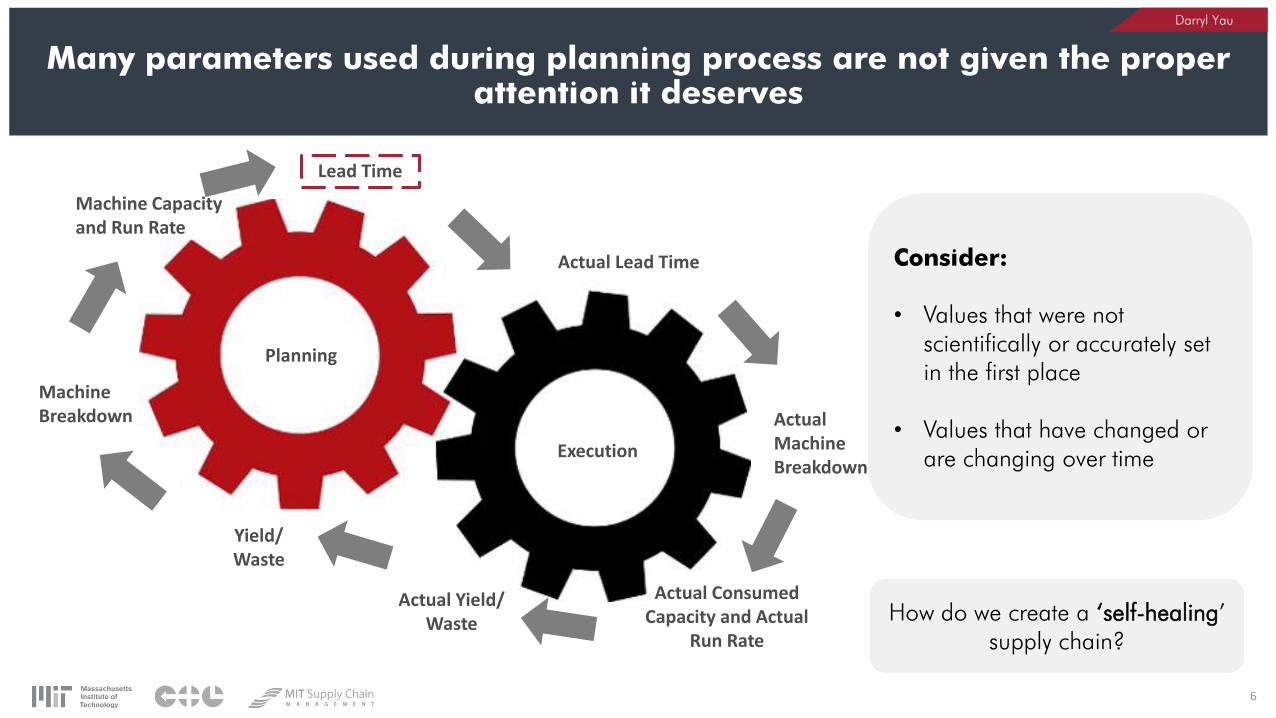
Many parameters used during planning process are not given the proper attention it deserves

6

Planning

Execution

Lead Time

Machine Breakdown

Yield/ Waste

Actual Lead Time

Actual Consumed Capacity and Actual

Run Rate

Actual Yield/ Waste

Machine Capacity and Run Rate

Actual Machine Breakdown

Consider:

• Values that were not

scientifically or accurately set

in the first place

• Values that have changed or

are changing over time

How do we create a ‘self-healing’

supply chain?

Darryl Yau

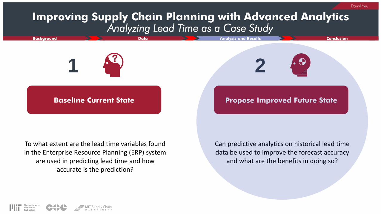
Improving Supply Chain Planning with Advanced AnalyticsAnalyzing Lead Time as a Case Study

To what extent are the lead time variables found in the Enterprise Resource Planning (ERP) system

are used in predicting lead time and how accurate is the prediction?

Can predictive analytics on historical lead time data be used to improve the forecast accuracy

and what are the benefits in doing so?

Baseline Current State Propose Improved Future State

1 2

Darryl Yau

Background Data Analysis and Results Conclusion

DataData

Background

Today’s Agenda

8

1

2

Analysis and Results3

Conclusion4

2

Data

Darryl Yau


Purchase Order Data (2004-2017)

9

Data

• Over 4M Line

Items (500,000+

Purchase Orders)

• Over 80,000

SKUs

Darryl Yau


Understanding Different Lead Time Variables Along the Planning Process

10

Planned Lead Time Actual Lead Time

Standard Lead-Time Variables

When Order is Placed

When Order is Received

Lead Time by SKU and Vendor (LTv)

Lead Time by SKU and Plant (LTp)

Other Business Constraints/

Decisions

Vs.

How can the accuracy be improved?

Data

Does not change over

time

Planning Process

Darryl Yau


Conceptualizing How Planned Lead Time is Formulated

11

𝑃𝑙𝑎𝑛𝑛𝑒𝑑 𝐿𝑒𝑎𝑑 𝑇𝑖𝑚𝑒𝑆𝐾𝑈−𝐿𝑎𝑛𝑒=𝑉1𝑃1 = β0+ β1𝐿𝑇𝑃1 +β2𝐿𝑇𝑉1 +

εWhere β

i= coefficients

ε = error or unexplained term

Data

Lead Time based on SKU and Plant

Vendors

V1

V1

V1

Plant

P1

P3

P2

Lead Time based on SKU and Vendor

LTv1

LTV1

LTV1

LTP3

LTP3

LTP3

LTP1

Darryl Yau


Analysis and Results

Data

Background


Today’s Agenda

12

1

2

3

Conclusion4

3


Darryl Yau








1 2


Darryl Yau


Regression Performed Across the Entire Dataset

14

β

β β


• Poor R2

values

• Seems to

improve over

time

• R2

values for

Actual Lead

Time

consistently

worse than R2

for Planned

Lead Time

LTv

and LTp

vs.

Planned Lead Time

LTv

and LTp

vs.

Actual Lead Time

Darryl Yau


Vendor and Plant appears to be factors contributing to the variability of actual lead time

15

Colored by Vendor Colored by Plant


Note: Using one SKU as an example

Darryl Yau


Analyses performed at the SKU-Lane level

16

Vendors(200+)

Plants(20+)

.

.

.

V1

Vn

P1

V2

V3

P2

P3

Pn

.

.

.

L1

Ln

Lanes(500+)


Lane = Unique Vendor and Plant Combination

Darryl Yau


t Test – Null Hypothesis: Are these datasets statistically the same?

17


• Ran t test on over

25,000 SKU-Lanes

• For LTv and

Planned Lead

Time

• For LTp and

Planned Lead

Time

• Planned Lead

Time and Actual

Lead Time

• NOT the same for all

tests

Darryl Yau








1 2

The standard lead time variables (LTv and LTp) are

not good predictors for what is planned

The planned lead times are not good predictors for

what actually happens


Darryl Yau








1 2


Darryl Yau


Time Series Analysis – Forecasting Methods

20

ො𝑥𝑡,𝑡+1 = 𝑥𝑡

ො𝑥𝑡,𝑡+1 =σ𝑖𝑡 𝑥𝑖𝑡

ො𝑥𝑡,𝑡+1 =σ𝑖=𝑡+1−𝑛𝑡 𝑥𝑖

𝑛

ො𝑥𝑡,𝑡+1 = 𝛼𝑥𝑡 + (1 − 𝛼)ො𝑥𝑡−1,𝑡

ො𝑥𝑡,𝑡+𝜏 = ො𝑎𝑡 + 𝜏𝑏𝑡

ො𝑎𝑡 = 𝛼𝑥𝑡 + 1 − 𝛼 (ො𝑎𝑡−1+𝑏𝑡−1)

𝑏𝑡 = 𝛽(ො𝑎𝑡−ො𝑎𝑡−1) + 1 − 𝛽 𝑏𝑡−1

ො𝑥𝑡,𝑡+𝜏 = ො𝑎𝑡 + 𝜏𝑏𝑡 + 𝐹𝑡+𝜏−𝑃

ො𝑎𝑡 = 𝛼(𝑥𝑡𝐹𝑡−𝑃

) + 1 − 𝛼 (ො𝑎𝑡−1+𝑏𝑡−1)

𝑏𝑡 = 𝛽(ො𝑎𝑡−ො𝑎𝑡−1) + 1 − 𝛽 𝑏𝑡−1𝐹𝑡 = 𝛾(

𝑥𝑡ො𝑎𝑡) + 1 − 𝛾 𝐹𝑡−𝑃

vs.


Darryl Yau


Bottom-up and Top-down Analyses

21

Individual SKU-Lane Analyses

Analyses on Entire Dataset


Darryl Yau


Analyzing one SKU-Lane

22


Darryl Yau


Forecasting on One SKU-Lane

23


Darryl Yau


Forecasting on One SKU-Lane

α

α β

α β γ

24


Darryl Yau


Bottom-up and Top-down Analyses

25

Individual SKU-Lane Analyses

Analyses on Entire Dataset


Darryl Yau


Analysis of Entire Dataset

26

Which had the Lower RMSE Result? (Forecast Method vs Baselines)

Mean MAPE of Forecast Methods vs. the Baselines


• Ran for over 2,500 SKU-Lane

Combinations

• Best Forecast Method had a lower

average MAPE than both baselines

• Using a single method had a lower

average MAPE than both baselines

• Best Forecast Method, on average,

performed better than both baselines

Darryl Yau


Which Forecast Method?

27


• Holt-Winter’s Method regularly

performed better than other

methods

• Holt’s Method regularly

performed worse than other

methods

Forecast Method with the Lowest RMSE Value (gaps not filled)

Holt’s

3%

100%

Naive

12%

Simple Exponential Smoothing

11%

Simple Mean TotalHolt-Winter’s

Moving Average (5)

8%

Moving Average (10)

42%

7%

17%

Darryl Yau


Trend did not appear to be a big factor in this dataset

28

15.0% 14.6% 13.0% 15.5%

85.0%96.5%

85.4% 87.0% 84.5%93.8% 94.3%

5.7%6.3%

Simple Mean

461

Naïve

307

3.5%

80

SES Holt’sMA (n=10)

1,117

Holt-Winter’s

MA (n=5)

199 278193100%

FalseTrue

10% Probability Series is Not Non-Stationary*

Of the five SKU-Lanes that

may have a trend in the data,

only 1 appeared to have a

significant trend.

*Based on Dickey-Fuller Test for Stationarity


Darryl Yau


Holt-Winter’s Method appears to perform well regardless of the level of seasonality in the data

29

33.3%36.4%

26.5%

41.0%44.7%

31.8%

6.1%

7.7%

7.8%

18.2%

12.2%

7.9%

7.1%

8.8%

66.7%18.2% 36.7%

12.4%

10.8%

11.4%

18.2%6.1%

12.4%

10.5%

9.7%

9.1%12.2%

20.0%15.9%

26.6%

3.2%

3.9%

4.8%

0

308100%

104060

1 11

50

3 1,973

30 20

29049

1.4%

Moving Average (5)

Naive

Holt’s

Simple Mean

Moving Average (10)

Simple Exponential Smoothing

Holt-Winter’s

Seasonality Percentages* (%)

*Based on Time Series Decomposition

Holt-Winter’s Method

appears to be a safe choice

regardless of seasonality

profile


Darryl Yau


Signs of ‘Lane Profile’

30


Certain Lanes

appear to favor

certain forecasting

methods

Lane ID

Darryl Yau


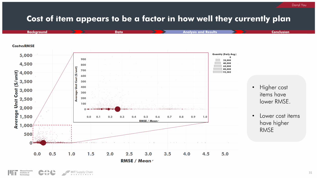
Cost of item appears to be a factor in how well they currently plan

31

31

• Higher cost

items have

lower RMSE.

• Lower cost items

have higher

RMSE


Darryl Yau


Financial Implications

32

Baseline 1:Planned

Lead Time

E[S

afe

ty S

tock

Cost

]

$189,412

Best Forecast Method

$240,695

-6.4%

Baseline 2:Regression

Analysis

-21.3%

$202,309

Estimated Safety Stock Costs

𝐸 𝑠𝑎𝑓𝑒𝑡𝑦 𝑠𝑡𝑜𝑐𝑘 𝑐𝑜𝑠𝑡 = 𝑐ℎ𝑘𝜎𝐷𝐿

𝜎𝐷𝐿 = 𝜇𝐿𝜎𝐷2 + 𝜇𝐷

2𝜎𝐿2

𝑐 𝑢𝑛𝑖𝑡 𝑐𝑜𝑠𝑡 𝑢𝑛𝑖𝑡ℎ ℎ𝑜𝑙𝑑𝑖𝑛𝑔 𝑟𝑎𝑡𝑒 𝑣𝑎𝑙𝑢𝑒 𝑡𝑖𝑚𝑒 𝐹𝑜𝑟 𝑡ℎ𝑖𝑠 𝑎𝑛𝑎𝑙𝑦𝑠𝑖𝑠 ℎ 𝑖𝑠

𝑎𝑠𝑠𝑢𝑚𝑒𝑑 𝑡𝑜 𝑏𝑒𝑘 𝑠𝑎𝑓𝑒𝑡𝑦 𝑓𝑎𝑐𝑡𝑜𝑟

𝜎𝐷𝐿𝜎𝑖 𝑠𝑡𝑎𝑛𝑑𝑎𝑟𝑑 𝑑𝑒𝑣𝑖𝑎𝑡𝑖𝑜𝑛 𝑜𝑓 𝑑𝑒𝑚𝑎𝑛𝑑 𝐷 𝑜𝑟 𝑙𝑒𝑎𝑑 𝑡𝑖𝑚𝑒 𝐿𝜇𝑖 𝑚𝑒𝑎𝑛 𝑜𝑓 𝑑𝑒𝑚𝑎𝑛𝑑 𝐷 𝑜𝑟 𝑙𝑒𝑎𝑑 𝑡𝑖𝑚𝑒 𝐿


Potential cost savings by reduction in

their safety stock

Darryl Yau


Bringing it together….

33

Planned Lead Time Actual Lead Time

Standard Lead-Time Variables

When Order is Placed

When Order is Received

Lead Time by SKU and Vendor (LTv)

Lead Time by SKU and Plant (LTp)

Other Business Constraints/

Decisions

Vs.

How can the accuracy be improved?

Does not change over

time

Planning Process

Predictive Lead Time Variable

Planned Lead Time(based on

Predictive LT)

Accuracy Improved


Darryl Yau








1 2

Using historical data to predict lead times can reduce

the error between plan and actual

Reduces Safety Stock costs and manual labor costs


Darryl Yau


Conclusion


Data

Background

Conclusion

Today’s Agenda

35

1

2

3

44

Conclusion

Darryl Yau


Conclusions and Considerations

36

Using Predictive Lead Time can reduce the error

between plan and actual

Safety Stock Cost

Manual Labor in PO Management

Manual Labor in Planning and Re-Planning

Consider:

Assigning Forecast Method by Lane

Implementing on High Volume, Low Cost Items

Categorizing SKU-Lanes by Trend, Seasonality

Conclusion

37

Questions?

Backup Slides

Darryl Yau

BackgroundBackground

Today’s Agenda

39

1

Data2

Analysis and Results3

Conclusion4

1

Darryl Yau


Industry 4.0

40

1784 – Mechanization,

water power, steam

power

1.0 4.03.02.0

1870 – Mass production,

assembly line, electricity

1969 – Computer and

automation

Present – Cyber physical

systems / digital transformation

Background

Important for 2 reasons:

1. Access to more data for analyses

2. Evolution of a “digital supply chain’s” role in planning

Darryl Yau


Digital Supply Chain

41

Web-basedReal-time

Cost Savings

Cloud

SensorsMonitoring

Visibility

Paperless

Background

Darryl Yau


‘Digital Copy’ implies a level of detail in their similarity

42

≈

Background

Supply Chain Planning Systems (e.g., ERP, APS) are becoming increasingly more complex in order to

more accurately model the complexities of the physical supply chain

Darryl Yau


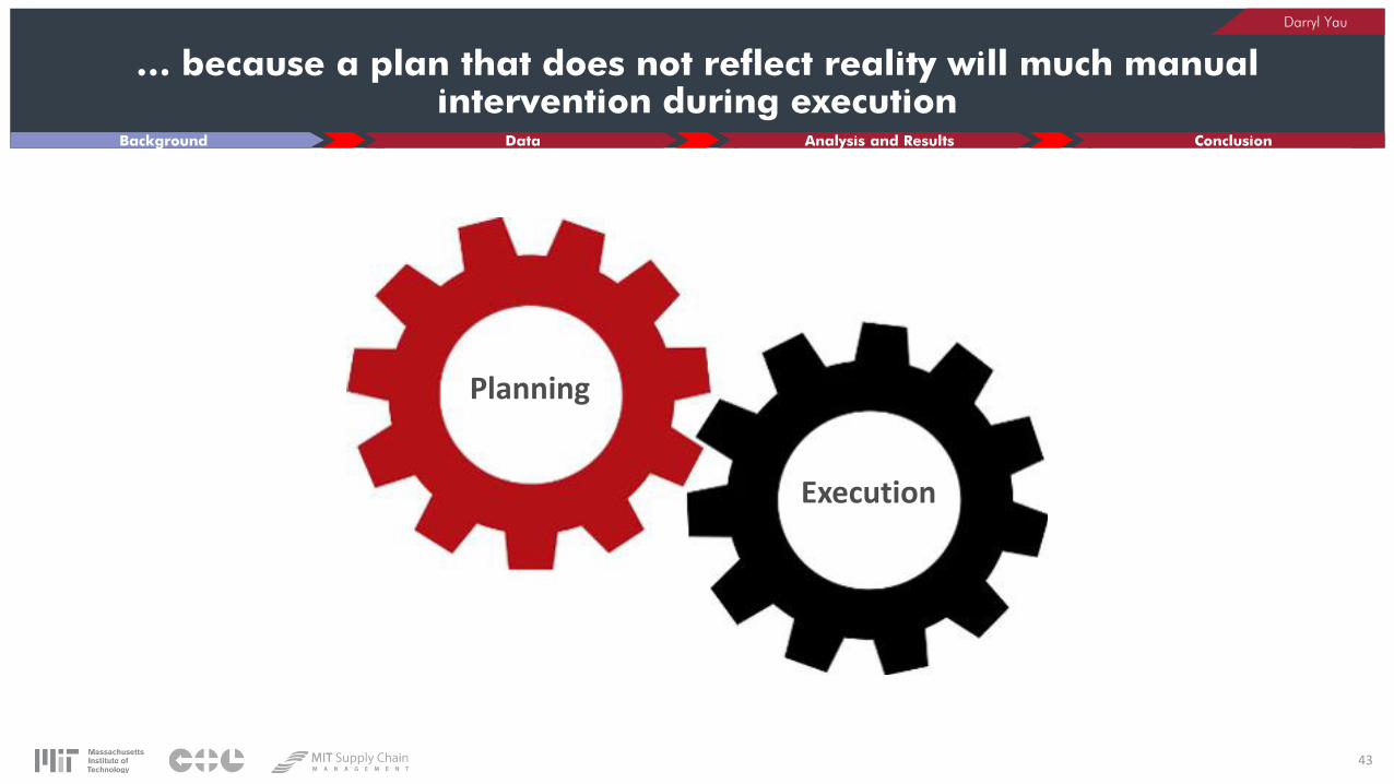
… because a plan that does not reflect reality will much manual intervention during execution

43

Planning

Execution

Background

Darryl Yau


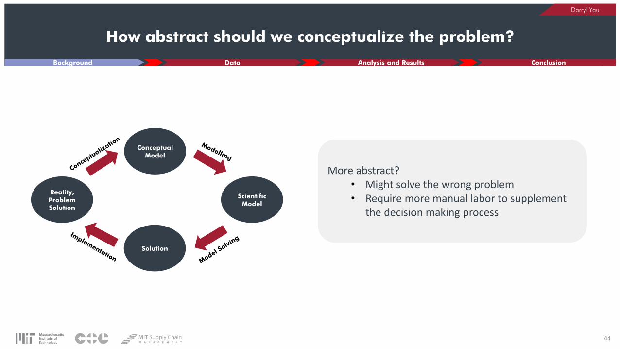
How abstract should we conceptualize the problem?

44

Conceptual Model

Solution

Scientific Model

Reality, Problem Solution

Background

More abstract? • Might solve the wrong problem• Require more manual labor to supplement

the decision making process

Darryl Yau


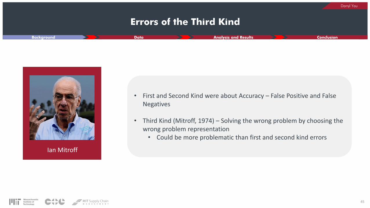
Errors of the Third Kind

45

Ian Mitroff

Background

• First and Second Kind were about Accuracy – False Positive and False Negatives

• Third Kind (Mitroff, 1974) – Solving the wrong problem by choosing the wrong problem representation• Could be more problematic than first and second kind errors

Darryl Yau


Humans Making Decisions?

46

Background

• Kahneman & Tversky, 1979

• Prospect Theory – People make decisions based

on potential value rather than the outcome

• Wu and Gonzalez, 1999

• Further studies on Prospect Theory. Analyzed

different probability weighting functions

• Schweitzer & Cachon, 2000

• Managers consistently deviated from the optimal

order point for newsvendor problem, even with

feedback and additional training

Darryl Yau


To Summarize…

47

We need a planning process that is:

Data Driven

Less Human InterventionMore Complex, More Like the Physical

improving supply chain planning with advanced analytics

Documents