implementation of steerable pyramids with …williams/ron-thesis.pdfimplementation of steerable...
TRANSCRIPT

Implementation of Steerable Pyramidswith Hexagonal Sampling
by
Ron L. Hospelhorn
B.S., Physics, California Institute of Technology, 1974
THESIS
Submitted in Partial Fulfillment of the
Requirements for the Degree of
Master of Science
Computer Science
The University of New Mexico
Albuquerque, New Mexico
December, 2006

c©2006, Ron L. Hospelhorn
iii

Acknowledgments
I would like to thank my adviser, Professor Lance Williams, for his support andtechnical advice.
iv

Implementation of Steerable Pyramidswith Hexagonal Sampling
by
Ron L. Hospelhorn
ABSTRACT OF THESIS
Submitted in Partial Fulfillment of the
Requirements for the Degree of
Master of Science
Computer Science
The University of New Mexico
Albuquerque, New Mexico
December, 2006

Implementation of Steerable Pyramidswith Hexagonal Sampling
by
Ron L. Hospelhorn
B.S., Physics, California Institute of Technology, 1974
M.S., Computer Science, University of New Mexico, 2006
Abstract
Multi-scale image processing frequently serves as the first step in scene analysis, pat-
tern recognition, texture analysis, image reconstruction, and many other early vision
tasks. A pyramid architecture analyzes an image independently at several scales, and
a steerable pyramid can extract oriented features at each of those scales. Hexagonal
sampling of image data promises processing economies over rectangular sampling as
well as higher angular resolution. This thesis discusses the implementation of filters
for hexagonally sampled data and uses them in two steerable pyramid designs.
vi

Contents
List of Figures x
List of Tables xiii
1 Introduction 1
1.1 Pyramid Decompositions . . . . . . . . . . . . . . . . . . . . . . . . . 1
1.2 Hexagonal Sampling . . . . . . . . . . . . . . . . . . . . . . . . . . . 8
1.3 Thesis Overview . . . . . . . . . . . . . . . . . . . . . . . . . . . . . . 12
2 Two Steerable Pyramids 15
2.1 Pyramid Processing Structures . . . . . . . . . . . . . . . . . . . . . . 15
2.2 Original Shiftable Steerable Pyramid . . . . . . . . . . . . . . . . . . 21
2.3 Standard Shiftable Steerable Pyramid . . . . . . . . . . . . . . . . . . 25
3 Filter Implementation 31
3.1 Overview . . . . . . . . . . . . . . . . . . . . . . . . . . . . . . . . . . 31
vii

Contents
3.2 Polar Fourier Transform (Analytical) Method . . . . . . . . . . . . . 35
3.3 Frequency Domain Resampling . . . . . . . . . . . . . . . . . . . . . 42
3.3.1 Hexagonal Sampling and Frequency Scaling . . . . . . . . . . 43
3.3.2 Fourier Transform of Hexagonally Sampled Series . . . . . . . 46
3.3.3 Forming a Hexagonal Fundamental Period . . . . . . . . . . . 49
3.3.4 The Hexagonal Fast Fourier Transform . . . . . . . . . . . . . 51
3.3.5 McClellan Frequency Transformation . . . . . . . . . . . . . . 53
3.4 Oriented Filters . . . . . . . . . . . . . . . . . . . . . . . . . . . . . . 56
4 Pyramid Reconstruction Accuracy 61
4.1 Accuracy of the Radial Filters . . . . . . . . . . . . . . . . . . . . . . 62
4.1.1 Reference Reconstruction Performance . . . . . . . . . . . . . 64
4.1.2 Accuracy of the Original Shiftable Pyramid . . . . . . . . . . 65
4.1.3 Accuracy of the Standard Shiftable Pyramid . . . . . . . . . . 68
4.2 Accuracy of the Oriented Filters . . . . . . . . . . . . . . . . . . . . . 70
4.2.1 Rectangular Standard Shiftable Pyramid Accuracy . . . . . . 71
4.2.2 Steerable Original Shiftable Pyramid Accuracy . . . . . . . . . 72
4.2.3 Hexagonal Standard Shiftable Pyramid Accuracy . . . . . . . 73
4.2.4 Additional Oriented Filters for the Original Shiftable Pyramid 74
5 Noise Reduction Using Local Orientation Analysis 79
viii

Contents
5.1 Application Overview . . . . . . . . . . . . . . . . . . . . . . . . . . . 79
5.2 Local Orientation Mapping . . . . . . . . . . . . . . . . . . . . . . . . 80
5.3 Noise Reduction Application . . . . . . . . . . . . . . . . . . . . . . . 88
5.4 Conclusions . . . . . . . . . . . . . . . . . . . . . . . . . . . . . . . . 93
6 Future Work 95
A Kernels 99
B Matlab/Octave Filter Code 106
B.1 Octave Code for Inverse Polar FT . . . . . . . . . . . . . . . . . . . . 107
B.2 Kernel Size Estimation . . . . . . . . . . . . . . . . . . . . . . . . . . 109
B.3 McClellan Transformation Scripts . . . . . . . . . . . . . . . . . . . . 110
B.4 HFFT Implementation . . . . . . . . . . . . . . . . . . . . . . . . . . 112
B.5 Formatting a Hexagonal Fundamental Period . . . . . . . . . . . . . . 115
B.6 Oriented Filter Kernels . . . . . . . . . . . . . . . . . . . . . . . . . . 117
B.7 Kernel Refinement . . . . . . . . . . . . . . . . . . . . . . . . . . . . 123
B.8 Accuracy Measurement . . . . . . . . . . . . . . . . . . . . . . . . . . 125
B.9 Miscellaneous Matlab/Octave Routines . . . . . . . . . . . . . . . . . 126
References 127
ix

List of Figures
1.1 Six level image pyramid with three orientations. . . . . . . . . . . . 2
1.2 Laplacian pyramid block diagram . . . . . . . . . . . . . . . . . . . 6
1.3 Possible symmetries for regular tilings. . . . . . . . . . . . . . . . . . 10
1.4 Hexagonally sampled image with hexagonal pixels . . . . . . . . . . 12
1.5 Expanded rectangularly sampled image . . . . . . . . . . . . . . . . 13
2.1 Block diagram of pyramid decomposition . . . . . . . . . . . . . . . 18
2.2 Initial low-pass filter L0 for original shiftable pyramid. . . . . . . . . 23
2.3 Recursion low-pass filter L1 for original shiftable pyramid. . . . . . . 24
2.4 Band-pass filter B for the original shiftable pyramid. . . . . . . . . . 24
2.5 Kernels for L1, L0, and radial BP . . . . . . . . . . . . . . . . . . . . 25
2.6 Initial low-pass filter L0 for standard shiftable pyramid. . . . . . . . 28
2.7 Recursion low-pass filter L1 for standard shiftable pyramid. . . . . . 28
2.8 Band-pass filter B for standard shiftable pyramid. . . . . . . . . . . 29
2.9 L0, L1, and radial BP kernels for standard shiftable pyramid. . . . . 29
x

List of Figures
2.10 Power sum of band-pass and recursion low-pass filters. . . . . . . . . 30
3.1 Two kernel construction methods for circular filters. . . . . . . . . . 32
3.2 Influence of 1-D kernel values on circularly symmetric kernel values. 37
3.3 Grid and coordinate system for hexagonal sampling . . . . . . . . . 43
3.4 Dimensions of band limited hexagonal region . . . . . . . . . . . . . 44
3.5 Hexagonal fundamental periods as a tiling of hexagons and equivalent
parallelograms. . . . . . . . . . . . . . . . . . . . . . . . . . . . . . . 47
3.6 Division of fundamental period hexagon into equivalent parallelogram. 50
3.7 Procedure for constructing an oriented kernel by analytical inverse
polar Fourier transform. . . . . . . . . . . . . . . . . . . . . . . . . . 58
3.8 Radial kernel profile as function of angular function order. . . . . . . 59
3.9 Procedure for constructing an oriented kernel by resampling method. 60
4.1 Images used for measuring reconstruction accuracy. . . . . . . . . . 63
4.2 Band-pass responses for 7, 13, and 20 hexagonal kernel layers. . . . . 66
4.3 “lena” image convolved with three cos2(θ) basis kernels. . . . . . . . 77
4.4 “lena” image convolved with six cos5(θ) basis kernels. . . . . . . . . 78
5.1 Square and hexagonal downsampling patterns for noise reduction
comparison. . . . . . . . . . . . . . . . . . . . . . . . . . . . . . . . 81
5.2 0 ◦ basis kernel for cos5(θ) oriented filter and its quadrature counter-
part. . . . . . . . . . . . . . . . . . . . . . . . . . . . . . . . . . . . 82
xi

List of Figures
5.3 “Cross” image used for orientation maps. . . . . . . . . . . . . . . . 84
5.4 Orientation maps at center, upper horizontal edge, right vertical edge
of the cross. . . . . . . . . . . . . . . . . . . . . . . . . . . . . . . . 85
5.5 Locations of orientation mapping points for “lena.” . . . . . . . . . . 86
5.6 Orientation maps at various points of “lena” image. . . . . . . . . . 87
5.7 Noise reduction by local orientation analysis. . . . . . . . . . . . . . 88
5.8 Hexagonal and square downsampled images with noise reduction. . . 91
5.9 Full resolution image with noise reduction. . . . . . . . . . . . . . . 92
xii

List of Tables
4.1 Accuracy of standard shiftable pyramid on rectangular grid . . . . . 64
4.2 Accuracy of original shiftable pyramid with analytical filters . . . . . 67
4.3 Accuracy of original shiftable pyramid with transformed filters . . . 67
4.4 Accuracy of standard shiftable pyramid with analytical filters . . . . 69
4.5 Accuracy of standard shiftable pyramid with transformed filters . . . 70
4.6 Accuracy of rectangular standard shiftable pyramid with cos(θ) . . . 71
4.7 Accuracy of rectangular standard shiftable pyramid with cos3(θ) . . 71
4.8 Accuracy of original shiftable steerable pyramid with cos(θ) . . . . . 73
4.9 Accuracy of original shiftable oriented pyramid with cos3(θ) . . . . . 74
4.10 Accuracy of oriented standard shiftable pyramid with cos(θ) . . . . . 75
4.11 Accuracy of oriented standard shiftable pyramid with cos3(θ) . . . . 76
4.12 Accuracy of original shiftable oriented pyramid with cos2(θ) . . . . . 76
4.13 Accuracy of original shiftable oriented pyramid with cos5(θ) . . . . . 77
A.1 Original Shiftable direct circular kernels . . . . . . . . . . . . . . . . 101
xiii

List of Tables
A.2 Original Shiftable direct oriented kernels . . . . . . . . . . . . . . . 102
A.3 Original Shiftable transformed circular kernels . . . . . . . . . . . . 103
A.4 Standard shiftable analytical kernels . . . . . . . . . . . . . . . . . . 104
A.5 Standard shiftable transformed kernels . . . . . . . . . . . . . . . . . 105
xiv

Chapter 1
Introduction
1.1 Pyramid Decompositions
Image scene analysis begins with processing that enhances and (possibly) isolates
image features. Such features occur in natural images at a number of spectral scales,
and the features at each scale should generally be processed separately. Decomposing
the image into component images which contain information specific to a particular
scale may be accomplished by passing the image through filters corresponding to the
scales of interest. Multiple orientations at each scale are similarly processed using
filters that are “tuned” for orientation.
Figure 1.1 shows a recursive pyramid decomposition with three orientation sub-
bands and six levels of scale [7, 22].
1

Chapter 1. Introduction
Figure 1.1: Six level image pyramid with three orientations.
2

Chapter 1. Introduction
The image processed through filters oriented at 0 ◦, 60 ◦, and 120 ◦ appears in
the upper left, upper right, and lower left quadrants, respectively. The lower right
quadrant contains the recursive pyramid of the same image filtered to prevent aliasing
and down sampled by a factor of two. Note that important image features disappear
and reappear from one orientation to another, and that this behavior persists over a
wide range of scales.
The preceding image set represents an encoding of the original image by a math-
ematical operator known as an overcomplete wavelet transform [22]. Although a
complete description of wavelet transforms cannot be offered here, a useful devel-
opment can be found in the textbook on image processing by Castleman [5]. This
source provides a number of insights about wavelet transforms that we can use to
build a case for the advantages of a pyramid algorithm for image processing. One
such insight is that a function may be represented as the weighted sum of basis func-
tions, or equivalently, the dot product of the weight coefficient vector and a vector
of basis functions. The set of weighting coefficients is known as the transform of
the function. If the function resembles one of the basis functions, then its transform
would be restricted to a small set clustered around the coefficient whose basis func-
tion matches it most closely. Looking at it another way, if we were to build a filter
bank comprising the set of basis functions and process the input function through
it, we would expect strong responses from the filters whose basis functions surround
the matching basis function, with the strongest response coming from the matching
basis function itself. Other filters would response weakly.
The Fourier series is the most familiar example of a transform for periodic (or
periodically extended) functions. The harmonic function eikωt, where k takes on all
integer values or the trigonometric functions sin(kωt) or cos(kωt), where k takes on
all nonnegative integer values, serve as the Fourier basis functions. The transform
of a function using the Fourier series is the set of Fourier coefficients. Similarly,
3

Chapter 1. Introduction
the continous Fourier transform uses the harmonic function parameterized in k as its
basis function but lets k take on a continuum of values [3]. Consequently, it produces
a continuous function as its transform, and represents the dot product as an integral
rather than a sum. The Discrete Fourier Transform (DFT) is the Fourier transform
of a function sampled at uniform intervals [5].
Whatever version of the Fourier transform we use, the basis functions are pe-
riodic functions of infinite extent. Naturally occurring signals, such as digitized
images, are functions which contain features of finite extent and do not resemble any
single Fourier basis function. The image function will therefore be represented by a
weighted sum of many basis functions, and its transform will therefore extend over
much of the transform space. One consequence of this fact is that the position of any
given feature cannot be easily read out from the transform. Another consequence
is that, since no basis function resembles an image feature, a filter bank built up of
the basis functions would not produce a response that would clearly select one basis
function over any of the others. Thus, the Fourier transform could not be easily used
to identify image features.
A wavelet transform attains the ability to both identify and locate signal features
by utilizing basis functions that resemble those features. The basis functions are
strongly localized in extent so that they can closely represent signal features of a
particular size. This being the case, the location of a basis function, which has no
meaning for harmonic functions, now matters. Wavelet basis functions therefore
specify both scale and location, so that from the preceding arguments, a set of such
basis functions could represent the salient features of an image very compactly if
designed correctly.
Intuitively, we would expect that a large feature matches with a basis function of
larger extent, and a small feature matches a basis function with smaller extent. This
follows from simple scaling, where we would want to apply the identical but scaled
4

Chapter 1. Introduction
basis function to an identical but scaled input function. That is, the transform is
scale invariant . When dealing with continuous transforms, scale may be handled
with the similarity theorem [3, 5]. However, the pyramid algorithms discussed in
this thesis deal exclusively with sampled image functions and therefore with discrete
transforms. A two-dimensional basis function that matches an image feature at a
small scale will require a2 the number of points to represent it when scaled to match
a similar feature that is a times larger. The number of points needed to represent the
smallest basis function is determined by the sampling interval required to perfectly
reconstruct the original image. By the Nyquist Sampling Criterion [3, 5], this is one
half the size of the smallest feature of interest. The image must be band limited
(its resolution controlled) so that the “smallest feature of interest” has the minimum
number of samples, or the image will not be reconstructed perfectly.
Processing an image repeatedly with scaled filters seems very wasteful on the face
of it. If a given resolution suffices for the smallest basis function, then a higher reso-
lution is unnecessary for the scaled up basis functions. Adelson et al [1] recognized
that a single filter applied to a set of scaled images produces the same result as scaled
filters applied to a single image. The Laplacian pyramid, which they devised and
which embodies this approach, uses a Gaussian basis function. The filter is applied
to the input image, which is repeatedly scaled by downsampling. Thus, the same
filter is applied to the same image at progressively larger scales.
In detail, the Laplacian pyramid transform works as follows. A low-pass Gaus-
sian filter blurs the input image before it is downsampled to produce a low-pass
subband. The low-pass subband image is then upsampled and passed through a
low-pass interpolation filter. The interpolated result is subtracted from the original
image and stored as the high-pass subband. The low-pass subband is processed by
the next pyramid stage, where it is again downsampled and filtered to produce the
next low-pass subband. To synthesize the input image from its Laplacian pyramid
5

Chapter 1. Introduction
representation, each stage is reconstructed by upsampling the previous low-pass sub-
band image, filtering it with the interpolation low-pass filter, and adding the resulting
image to the high-pass subband image stored in the next stage of the pyramid. The
process continues until the pyramid is exhausted, leaving the original image.
The diagram in Figure 1.2 shows a Laplacian pyramid as presented by Simoncelli
and Adelson [24] in an article on subband transforms. The dot labeled as w0(n) rep-
resents the next recursive stage, replicating the function of the entire diagram. As
Figure 1.2: Laplacian pyramid block diagram
Adelson points out [1, 24], the pyramid reconstructs the original image exactly, inde-
pendent of the choice of filters, since the pyramid stores the difference of the image
and the upsampled and interpolated reconstruction of the next stage. Most pyramid
designs depend upon closely matched filters for accurate image reconstruction, so
the Laplacian pyramid is unusual in that respect.
As discussed previously, wavelet transforms use basis functions with compact
support in both the space and transform domains. That is, a feature that is well
localized in the space domain will also be well localized in the transform domain. A
6

Chapter 1. Introduction
wavelet function is designed to match a particular type of feature, such as a line or
edge, with a very few basis functions. Since the action of the transform occurs at a
particular scale, and it is necessary to analyze the image for similar features at larger
and smaller scales as well as different locations, wavelet functions are derived from
a single prototype function by dilation and translation [5].
Dyadic wavelet transforms, that is, wavelet transforms whose basis functions
scale by a factor of two, lend themselves to pyramid decompositions. Pyramid im-
plementations of orthonormal wavelets in particular have proven useful in encoding
applications [22]. The chief advantage of the orthogonal wavelet pyramid is that
it can be implemented very economically. The transformed image contains exactly
the same number of pixels as the input image, and the transform is self-inverting.
Orthogonality is achieved by downsampling and filtering both the low and high fre-
quency subbands [5]. Downsampling the high frequency subband introduces aliasing.
However, the orthogonal transform is designed to ensure that aliasing errors from all
the subbands cancel upon reconstruction of the image. Image coding and transmis-
sion applications can tolerate subband aliasing, so long as the image is reconstructed
accurately. Other applications require aliasing-free subbands so that each subband
can be processed accurately and independently of the others.
As demonstrated by Simoncelli et al [22], subband aliasing transfers information
among subbands when the input signal is shifted by translation, dilation, or rotation.
In order to avoid this, the transforms must abandon orthogonality. In fact, orthogo-
nality, and with it, critical sampling, can no longer be tolerated. Applications which
must avoid subband aliasing require sampling at a rate in excess of the Nyquist rate.
This thesis describes the implementation of steerable pyramids. These filter struc-
tures depend on shiftability in angular orientation and must utilize low-pass filters
at each decomposition stage to eliminate aliasing from downsampling. Because the
transforms are shiftable in orientation, a set of basis filters can synthesize a filter
7

Chapter 1. Introduction
with any desired orientation. This property is termed steerability . We present two
steerable pyramid designs to illustrate the problems encountered in designing and
implementing steerable pyramids. The first pyramid figures prominently in Simon-
celli’s paper on shiftability [22]. This paper shows that a shiftable pyramid must
use the Nyquist sampling rate at each stage and explains how and why steerable
filters function. The second pyramid uses filters developed by Karasaridis and Si-
moncelli [10] to illustrate a technique to filters that accurately meet pyramid design
constraints.
More to the point, this thesis describes the implementation of the two pyramids
with filters defined on hexagonal grids. Filters can be constructed from general
specifications by calculating each hexagonal grid point of the basis function (referred
to as the kernel or impulse response in the following) from one-dimensional transfer
functions. Alternatively, filters on a hexagonal grid can be copied from existing filter
kernels on a rectangular-grid by resampling the kernels. Future work with pyramids
using hexagonal filters will be able to use our results to produce accurate filters with
little effort.
1.2 Hexagonal Sampling
The pyramid analysis framework simplifies the use of steerable filters in a number of
image processing applications, including local orientation analysis, corner identifica-
tion, noise suppression, oriented feature enhancement, shape from shading analysis,
and others [7, 22]. It is our opinion that these applications can benefit from the
increased angular resolution and computational economies that the use of hexagonal
sampling grids promises.
The general sampling theorem developed by Mersereau [14] depends on the pe-
riodic extension of a band limiting region R. This requirement is analogous to the
8

Chapter 1. Introduction
observation [5] that sampling a function on a square grid amounts to convolving it
with the Shah function, so that the Fourier transform of the function is replicated
over the entire frequency plane at intervals of 1/τ , where τ is the sampling interval.
If the function is sampled at the Nyquist rate or higher, its band limiting regions
will not overlap. The Fourier transform of the analogous sampling function for a
hexagonal grid covers the frequency plane with hexagons. The sampling theorem
states that if a two-dimensional function contains no frequency components outside
one such hexagon R, then it can be perfectly reconstructed from samples taken on
the corresponding sampling grid. From the preceding arguments it is clear that R
must be chosen such that it represents a single period of a periodic function. That
is, translated copies of R must cover the Fourier plane with no overlaps and no gaps,
thereby tessellating the plane. Mersereau calls this an admissible tiling . Regular ad-
missible tilings cover the plane with congruent polygons. Only squares, equilateral
triangles, and regular hexagons can tile the plane with a regular tesselation [8, 14].
Other admissible tilings are possible, using for instance, irregular or non-convex poly-
gons, but finding the corresponding sampling strategies presents a challenge beyond
the scope of this thesis.
The hexagonal grid possesses the highest possible symmetry of any regular sam-
pling geometry, and the implications of that fact motivate this thesis. A hexagon
offers 12-fold redundancy in coefficients as opposed to the 8-fold redundancy of a
square, or the 6-fold redundancy of a triangle. Figure 1.3 illustrates the respective
symmetries for an equilateral triangle (D3 symmetry), a square (D4 symmetry) and
a hexagon (D6 symmetry). The symmetry group names denote “dihedral” sym-
metry, in which each bisecting line in the diagram represents a plane of reflection.
In applications where symmetry is important, the redundancies due to symmetry
equate to savings in computational work. The high order of symmetry produces
related benefits. One important advantage of the hexagonal grid is that each point
has six nearest neighbors equidistant from it, as opposed to a point in a square grid,
9

Chapter 1. Introduction
Figure 1.3: Possible symmetries for regular tilings.
which only has four equidistant nearest neighbors. Each of the nearest neighbors in
a hexagonal grid aligns on an axis which contains samples spaced at the minimum
sampling interval, so that there are three of these axes compared to only two such
axes for the square grid. These properties of the hexagonal grid lead one to suspect
that it offers higher angular resolution and thus smaller aliasing errors for image
features not aligned with an axis. Therefore, diagonal features appear cleaner to the
eye when sampled hexagonally without the “jags” usually seen in images sampled on
a square grid. Importantly, applications which depend on the accuracy of local ori-
entation measurement can be expected to benefit from the higher angular resolution,
as well.
10

Chapter 1. Introduction
The hexagonal grid provides the highest number of samples for a given nearest
neighbor distance, i.e., the highest sampling density . Equivalently, the hexagonal
grid allows the highest nearest neighbor distance for a given number of samples in a
given area. Mersereau [14] points out that exact reconstruction of a circular region
using a hexagonal grid requires 13.4 percent fewer samples than with a rectangular
grid. He also notes that having six nearest neighbors all of which are equidistant as
opposed to only four equidistant neighbors for the rectangular grid can facilitate clus-
ter separation (deciding which points belong to which cluster, if any) and boundary
tracing applications.
Middleton and Sivaswamy [15] claim that hexagonal sampling together with
hexagonal pixels can improve the appearance of curves and diagonal edges to the
human eye. Figure 1.4 presents the famous “lena” image resampled on a hexagonal
grid and where each sample is rendered by a hexagon. Facial contours and diagonal
edges indeed appear to conform to what the eye expects with relatively little artifacts
due to the sampling geometry. The enlarged portion of the image reveals the struc-
ture of the sampling pattern. Curved areas appear to be well filled, and diagonals
do not display the jagged appearance associated with use of a rectangular grid. In
contrast, the enlarged rectangularly sampled image in Figure 1.5 exhibits artifacts
readily apparent to the eye and which are pronounced on diagonals and curves.
As a final note, it is well known that hexagonal patterns occur in natural vision
systems such as the compound insect eye [14]. Hexagonal packing places the highest
number of sensors within an area for a given sensor size than is possible with any
other arrangement, thus increasing sensor redundancy. It is also possible that the
neural processing of visual data benefits from the high order of symmetry offered by
hexagonal sampling. Discovering the signal processing in these natural systems is of
course a worthwhile end in itself. As in other technical fields that have benefitted
by emulating natural systems, it is likely that signal processing as well as pattern
11

Chapter 1. Introduction
Figure 1.4: Hexagonally sampled image with hexagonal pixels
recognition could gain by adopting the designs that have resulted from millions of
years of natural selection.
1.3 Thesis Overview
This thesis will present the detailed implementation of steerable pyramid image de-
compositions using image data sampled on hexagonal grids. In order to illustrate
12

Chapter 1. Introduction
Figure 1.5: Expanded rectangularly sampled image
specific issues involved in designing pyramid algorithms, Chapter 2 will compare
two designs taken from papers by Simoncelli and others [10, 22]. The first of these
papers introduces the theory behind shiftable steerable pyramids, while the second
describes a general method for designing filters for use in steerable pyramids. The
filters developed in the latter paper serve as standards for reconsruction accuracy.
The third chapter deals with computation and implementation of hexagonal filters
from general design specifications or from existing filters when a performance com-
parison is required. In this thesis we use both analytical (polar Fourier transform)
13

Chapter 1. Introduction
[13, 23] and resampling [12, 13] methods for computing filter coefficients. While the
analytical method does not require detailed consideration of hexagonal sampling or
Fourier transformation on the hexagonal grid, the second class of methods requires
both. Therefore, hexagonal sampling and Mersereau’s [14] Hexagonal Fast Fourier
Transform (HFFT) are discussed in Chapter 3.
The research described in this thesis uses steerable filters that are separable in
polar coordinates. The two-dimensional transfer function results from multiplying a
radial transfer function by the desired angular transfer function [3, 7]. A filter kernel
may be derived from the inverse Fourier transform of this product. It may also be
derived analytically by summing the inverse polar Fourier transform for each term of
the Fourier series of the angular function. In general, it is expected that the accuracy
of the oriented filter is limited by the accuracy of the radial filter upon which it is
based, since the angular function comprises a known and usually small number of
Fourier terms. Surprisingly, this is not always the case. The fourth chapter will
discuss the relationship between pyramid design, filter design, and reconstruction
accuracy. Reconstruction accuracy depends on the accuracy of the filter set, which
depends in turn on pyramid requirements. The tradeoffs involved and a curious
synergy will become apparent.
Hexagonal sampling places six neighbors around a given point, giving an angular
interval of 60 ◦. In contrast, square sampling surrounds each point with only four
nearest neighbors, giving an angular interval of 90 ◦ between them. This fact leads
to the supposition that the hexagonal sampling geometry represents small angles
more accurately than square sampling. Chapter 5 presents a simple application
that attempts to exploit this property of hexagonal filters to produce a measurable
improvement over rectangular filters in removing noise from an image.
14

Chapter 2
Two Steerable Pyramids
2.1 Pyramid Processing Structures
The two pyramids which we describe in this thesis share a common structure but
differ in the filters they employ. The following brief description of the pyramid
design applies to both. Both start with an initial high-pass filter operation that
subtracts a low-pass filtered image from the original image. The image is processed
twice by the low-pass filter so that the result, when subtracted from the original
image, achieves power complementarity with the pyramid output. The high-pass
filtered image that results comprises the first level of the pyramid, while the input
image low-pass filtered only once serves as input to the next stage of the pyramid.
For each succeeding stage of the pyramid, the input image is processed by both a
set of oriented band-pass filters and the anti-aliasing low-pass filter used at each
stage. The low-pass filtered image again serves as input to the next pyramid stage,
while the images output from the oriented band-pass filters represent the transform
result for the current pyramid level. When the desired number of decompositions
is reached, the application can perform any desired processing on the stored band-
15

Chapter 2. Two Steerable Pyramids
passed images. The original image can be reconstructed from the transform images
stored in the pyramid by upsampling the lowest image in the pyramid, convolving it
with the inverse of the low-pass filter used in downsampling, and then adding it to
the band-passed image at the next level of the pyramid. The same reconstruction
procedure could be applied to the pyramid after processing one or more of its images
with some operation such as wavelet coring for noise reduction, thus producing an
enhanced image.
Each stage of a pyramid comprises a filter bank which analyzes an input image
into basis images representing the transform of the scaled image with a basis func-
tion. The original image is reconstructed using another set of filters that invert the
transforms and synthesize the input image by combining the filter outputs. Thus,
a pyramid transform and its inverse is usually depicted with a diagram showing a
set of analysis/synthesis filter banks. Accurate image reconstruction requires that
each stage of the pyramid must be self-inverting in the sense that processing the
signal through both the analysis filters and the synthesis filters that invert them
results in a signal at the output that closely resembles the signal at the input. In
the following, we will refer to the pyramid presented in the Simoncelli, et al paper
on shiftability [22] as the original shiftable pyramid . The pyramid presented in the
paper by Karasaridis and Simoncelli [10] will be designated the standard shiftable
pyramid . The desired action of each stage for the original shiftable pyramid is to
filter the image with the overall system transfer function. The standard shiftable
pyramid requires constant power response for each stage over the frequency range of
interest.
The wavelet transforms implemented by both pyramids are overcomplete by a
factor of 4/3 for filters with circular symmetry. That is, the number of coefficients
in the pyramid representation is 4/3 times the number of values in the input image
[22]. The size of the pyramid representation is a power series in four, so that the
16

Chapter 2. Two Steerable Pyramids
total number of coefficients in the representation is approximately 4/3 the number
of values in the input image. A steerable pyramid with four oriented basis functions
per stage would have an overcompleteness factor of 16/3, since each band-pass filter
would be replaced by four oriented band-pass filters. However, to analyze the entire
pyramid, we observe that the transforms from the oriented band-pass filters are
inverted and combined to form a single band-passed image transform, so that the
overcompleteness of the pyramid representation can be regarded as 4/3 at each stage.
Since the transform is overcomplete, it doesn’t offer the efficiency of an orthogonal
transform, and the question arises as to its invertibility. Simoncelli et al [22] prove
that a transform that is shiftable and has an overall power response that is constant at
each stage is not only invertible, but is self-inverting. The property of self-invertibility
requires the transform to be a tight-frame. The fact that the transform is a tight-
frame implies two more interesting facts. One is that the inverse must be scaled by
the inverse of the overcompleteness factor. The other is that the inverse transform is
the transpose of the transform [6]. The overcompleteness factor must be compensated
in practice by scaling the reconstructed image at each stage by a factor of 1/4. This
is equivalent to observing that the synthesis stage image must be multiplied by 1/4
in order to compensate for upsampling, which multiplies the intensity of the image
by 2 in each direction. The total intensity of the final reconstructed image is thereby
multiplied by 4/3, thus compensating for the inherent transform scaling factor of
3/4.
Self-invertibility imposes constraints on the transfer functions of the component
filters. The accuracy with which the filters meet these constraints determines the ac-
curacy of the reconstructed image. Simoncelli et al [22] show that the self-invertibility
of the stage implies the self-invertibility of the component filters in that the sum of
their power responses must be the desired power response of the stage over the
frequency range of interest. That is, they are power complementary . The power
17

Chapter 2. Two Steerable Pyramids
complementarity equations define one of the constraints on the pyramid filters at
each stage and will be presented in the following sections with their respective pyra-
mid descriptions. These equations show that the filters are designed so that they
are inverted by their conjugate transposes. The radial filters are purely real and
symmetrical, so that they are self-inverting. The oriented filters are either purely
real or purely imaginary and so are inverted by their transposes.
Figure 2.1 presents a system diagram of the recursive analysis/synthesis filter
bank. This diagram is adapted from Karasaridis and Simoncelli [10], and applies to
both pyramid designs. The small box containing the black dot represents the next
(recursive) stage of the pyramid, and can be pictured as containing a copy of the
diagram within the dashed box.
Figure 2.1: Block diagram of pyramid decomposition
An important and necessary consequence of shiftability is that any value of the
sampled function may be derived from the values of surrounding sampled points by
interpolation. That a set of basis functions is shiftable in angular orientation means
that a filter with arbitrary angular orientation can be constructed by interpolating
from sampled values of the transfer function of the basis filters that span them.
18
Chapter 2. Two Steerable Pyramids
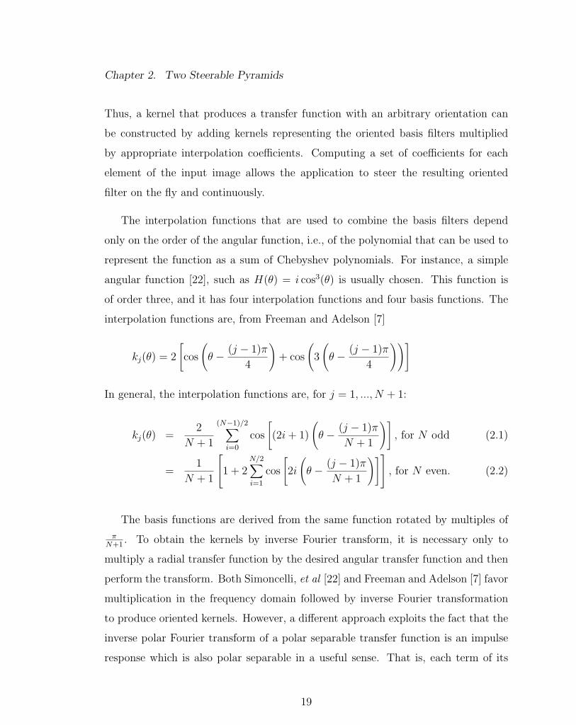
Thus, a kernel that produces a transfer function with an arbitrary orientation can
be constructed by adding kernels representing the oriented basis filters multiplied
by appropriate interpolation coefficients. Computing a set of coefficients for each
element of the input image allows the application to steer the resulting oriented
filter on the fly and continuously.
The interpolation functions that are used to combine the basis filters depend
only on the order of the angular function, i.e., of the polynomial that can be used to
represent the function as a sum of Chebyshev polynomials. For instance, a simple
angular function [22], such as H(θ) = i cos3(θ) is usually chosen. This function is
of order three, and it has four interpolation functions and four basis functions. The
interpolation functions are, from Freeman and Adelson [7]
kj(θ) = 2
[cos
(θ − (j − 1)π
4
)+ cos
(3
(θ − (j − 1)π
4
))]
In general, the interpolation functions are, for j = 1, ..., N + 1:
kj(θ) =2
N + 1
(N−1)/2∑i=0
cos
[(2i + 1)
(θ − (j − 1)π
N + 1
)], for N odd (2.1)
=1
N + 1
1 + 2N/2∑i=1
cos
[2i
(θ − (j − 1)π
N + 1
)] , for N even. (2.2)
The basis functions are derived from the same function rotated by multiples of
πN+1
. To obtain the kernels by inverse Fourier transform, it is necessary only to
multiply a radial transfer function by the desired angular transfer function and then
perform the transform. Both Simoncelli, et al [22] and Freeman and Adelson [7] favor
multiplication in the frequency domain followed by inverse Fourier transformation
to produce oriented kernels. However, a different approach exploits the fact that the
inverse polar Fourier transform of a polar separable transfer function is an impulse
response which is also polar separable in a useful sense. That is, each term of its
19

Chapter 2. Two Steerable Pyramids
expansion as a Fourier series in the angular function is polar separable. Stein and
Weiss [23] show that if f0(r) is a circularly symmetric function, z = reikθ, and
f(z) = f0(r)eikθ,
then the Fourier transform of f(z)
f(w) = F0(R)eikφ
F0(R) = 2π(−i)k∫ ∞
0f0(r)Jk(2πRr)rdr, (2.3)
where w = Reiφ, F0(R) is the radial component of the polar separable Fourier trans-
form function f(w), and Jk(x) is the kth order Bessel function of x. The transform
is self-inverting, since the inverse Fourier transform is obtained by changing the sign
of the Bessel function order and the power of the imaginary factor. These changes
produce the same expression as the forward transform. The impulse response for the
ith oriented basis function is computed by applying the preceding transformation
to each term of the Fourier expansion of the angular function and multiplying it by
cos(k(θ − θi)), where θi is offset angle of the i-th basis function and k is the order
of the Fourier term. Further details of implementing the analytical impulse response
calculation will be presented in Chapter 3.
The analytical method described in Chapter 3 offers the advantage of computa-
tional clarity and accuracy that is limited only by the size of the kernel. Unfortu-
nately, for a given accuracy, the analytical method produces kernels that are larger
than can be obtained by other methods. Use of larger kernels not only results in
an increased computational load, but the edge effect that results when the kernel
approaches the image in size limits the number of decomposition levels from which
an image can be reconstructed.
The two pyramid transforms presented here differ in the methods used to design
their component filters as well as the constraints they impose. The first design
emphasizes band limiting to obtain oversampling of the input and effective invariance
20

Chapter 2. Two Steerable Pyramids
to translations and rotations of the input image. Requirements imposed on the low-
pass filters determine the constraint on the band-pass filter, and it requires only
a single computation to determine its ideal transfer function. Given the size of
kernel desired and this transfer function, an optimization procedure can be used to
determine the impulse response [22]. The second pyramid transform comes from a
paper that presents a method of designing filters for pyramid transforms [10] that
produces the required frequency responses by an iterative design procedure that
minimizes filter errors over the frequency range of interest. The resulting filters are
posted online by Simoncelli [20]. Their availability and quality suggest their use as
a standard for comparing reconstruction accuracy, and they were used that way in
this study. These filters implemented on a rectangular grid achieved variance errors
as low as -63.6 dB. Results for the same filters on a hexagonal grid approached this
level of accuracy and exceeded it in some cases.
2.2 Original Shiftable Steerable Pyramid
Simoncelli, et al [22] developed a shiftable steerable pyramid design. This over-
sampled transform, while not completely translation invariant, avoids transferring
energy between subbands upon translation or rotation of the input image. Thus,
each subband can be processed independently without introducting aliasing. Just
as importantly, exact interpolation between translated or rotated samples follows
from shiftability. For steerable filters, this means that an oriented filter of any de-
sired orientation can be constructed from a small number of basis filters at fixed
orientations.
As stated in the Introduction, the transfer function of any two-dimensional band-
pass filter is assumed to be polar separable, so that its angular component can be
designed and implemented separately from its radial component. A one-dimensional
21

Chapter 2. Two Steerable Pyramids
specification can describe the radial component of the transfer function, and oriented
filters can be derived by multiplying the radial transfer function by the angular
function desired. Since the reconstruction of the oriented basis images equates to
the image obtained by processing the input image with a circularly symmetric band-
pass filter, the pyramid constraints apply to this filter and to the low-pass filters,
which are also circularly-symmetric.
The constraints of this pyramid transform permit very straightforward filter spec-
ifications. The transform differs from the transform represented by the second pyra-
mid in that a single stage of the pyramid recursion acts as a low-pass filter, and the
entire system has the same response as a single stage. The overall system response
L0(ω), has a power spectrum |L0(ω)|2 that is simply the sum of the band-pass filter
power |B(ω)|2 and the system response of the next lower recursion stage after it has
been passed through the recursion low-pass filter L1(ω).
|L0(ω)|2 = |B(ω)|2 + |L1(ω)|2|L0(2ω)|2 (2.4)
In the preceding equation, |B(ω)|2 is the sum of the powers |B0(ω)|2 and |B1(ω)|2 of
the oriented filters shown in the diagram. The L0(ω) system response at each stage
filters out aliasing that results from downsampling, so that the L1(ω) response can
be implemented by a relatively simple filter. The authors used
[1 6 15 20 15 6 1
]/64
as the kernel for L1(ω). They specified the overall system response L0(ω) indepen-
dently as a filter that has unity response from ω = 0 to ω = π/2 radians and zero
response at ω = π. Simoncelli et al [22] used the Parks-McClellan algorithm, im-
plementations of which may be found online [2], to find the thirteen-tap low-pass
filter which most nearly satisfies these criteria. This thesis used the online algorithm
to find a similar low-pass filter which most nearly satisfies the stated criteria. The
22

Chapter 2. Two Steerable Pyramids
Figure 2.2: Initial low-pass filter L0 for original shiftable pyramid.
transfer function produced by a ten-tap filter resulted in two-dimensional filters with
good accuracy for either method of filter construction used by this thesis. Figure 2.2
and Figure 2.3 show the respective transfer functions L0(ω) and L1(ω).
Given the two low-pass filters, L0(ω) and L1(ω), the band-pass filter transfer
function B(ω) is fully determined. Unfortunately, the required transfer function,
shown in Figure 2.4, is difficult to realize with compact support. The authors used
the Nelder-Mead [17] simplex optimization method to find a fifteen-tap filter whose
transfer function matches the ideal transfer function to within approximately 3.5
percent in power. As described in Chapter 3, two different methods yield a band-
pass filter with similar performance. Figure 2.5 shows the two low-pass kernels and
the radial band-pass kernel used in this thesis for the original shiftable pyramid.
Once the three one-dimensional filters have been designed, they can be used to
specify cross-sections of circularly symmetric two-dimensional filters and tested for
accuracy. Chapter 3 presents two methods for converting a one-dimensional kernel
23

Chapter 2. Two Steerable Pyramids
Figure 2.3: Recursion low-pass filter L1 for original shiftable pyramid.
into a two-dimensional kernel. The central cross-section of the circularly symmetric
transfer function produced by the two-dimensional kernel is the transfer function
of the one-dimensional kernel. The two-dimensional kernel can be derived from the
Figure 2.4: Band-pass filter B for the original shiftable pyramid.
24

Chapter 2. Two Steerable Pyramids
Figure 2.5: Kernels for L1, L0, and radial BP .
one-dimensional transfer function by numerical integration of the of the polar Fourier
transform or by Fourier transforming the result of frequency resampling the two-
dimensional transfer function. The latter is best accomplished by computing samples
of the transfer function on a hexagonal grid from a one-dimensional transfer function.
Chapter 3 describes the numerical integration in detail and proposes the McClellan
frequency transformation as the preferred technique for producing a resampled two-
dimensional transfer function.
2.3 Standard Shiftable Steerable Pyramid
The second steerable pyramid design comes from a paper by Karasaridis and Si-
moncelli [10] that presents a design technique for filters used in steerable pyramid
transforms. Kernels derived for it are available online at [20]. The site’s author
warns that the filters supplied with the C code “are not very accurate,” but they
appear identical to those supplied with the same application written in Matlab code
and which are supplied without this qualification.
Karasaridis and Simoncelli [10] present a pyramid whose circularly symmetric
filters on a rectangular grid achieve a image reconstruction error measured as -63.6 dB
25

Chapter 2. Two Steerable Pyramids
variance. The same pyramid with steerable filters achieves reconstruction accuracy
comparable to that reported in the source paper. These comparatively good results
are achieved using relatively small kernels. Evidently, the method produces very
accurate filters, but they are obtained at the cost of multiple rounds of optimization
[10]. For this thesis, we decided to simply copy the available filters rather than use
the design technique. Chapter 3 presents the details of how the filters are adapted
from a rectangular grid to a hexagonal grid.
The second pyramid design shares the overall structure of the first, but the de-
tailed design of the filters differs in important respects. The filter design procedure
for the second pyramid produces filters that match the pyramid requirements accu-
rately with compact support. The first pyramid, by way of comparison, also uses
relatively small kernels, but its accuracy is not as good.
As with the first pyramid, the image is low-pass filtered before being downsampled
and delivered to the next stage. The image is filtered a second time with the initial
low-pass filter and subtracted from the original image. The difference image, which
is put onto the top of the pyramid, is power complementary to the image returned
by the last stage of the synthesis filter when the image is reconstructed, since the
low-pass filter is applied once during the decomposition and again as the final step
in reconstruction. Rather than low-pass filtering and differencing with the original
image, the image could instead have been passed through a complementary high-pass
filter. However, that method was not used for this work.
The downsampled image is processed by a set of oriented band-pass filters and by
the anti-aliasing low-pass filter that is used at each stage. The outputs of the band-
pass filters constitutes the subbands that are stored for the current stage, just as for
the “original shiftable” design. The low-passed image continues to downsampling
and the next stage.
26

Chapter 2. Two Steerable Pyramids
The constraints on the filter transfer functions are as follows, where L0(ω) repre-
sents the response of the initial low-pass filter, L1(ω) represents the recursive low-pass
filter, and B(ω) represents the band-pass filter, or equivalently, the square root of
the sum of the oriented band-pass filter power responses:
|L0(ω)|2[|L1(ω)|2 + |B(ω)|2] = 1
|L1(ω/2)|2[|L1(ω)|2 + |B(ω)|2] = |L1(ω/2)|2
L1(ω) = 0, for |ω| > π/2.
The last condition is necessary in order to suppress aliasing due to downsampling of
the image. As an additional condition, L0(ω) is set equal to L1(ω/2), since L1(ω/2)
acts as the initialization filter L0(ω) for each recursive stage.
In contrast to the first pyramid, which presented the same low-pass filter transfer
function at each stage, this pyramid presents a constant transfer function up to
the cut-off frequency of the initial low-pass filter. Above that frequency, the transfer
function is irrelevant. The recursive low-pass filter and the band-pass filter are power
complementary to one another within this frequency range, and the band-pass filter
transfer function above this cutoff is unconstrained and can be implemented using any
convenient filter kernel with the required transfer function below the cutoff frequency.
Figure 2.6 through Figure 2.8 show the transfer functions of the filters. Figure 2.9
shows the kernels for these three filters. Figure 2.10 shows the sum of the squared
amplitudes of the recursive low-pass filter and the band-pass filter.
The set of filters for this standard shiftable pyramid served as a benchmark for
reconstruction accuracy in evaluating the filter implementation techniques described
in this thesis. As will be shown in Chapter 4, reconstruction accuracy on a hexag-
onal grid approaches the accuracy reported in [10] and measured here for the same
filters implemented on a rectangular grid. Chapter 4 presents measurements of re-
construction accuracy for both pyramid transforms, using filters constructed with
27

Chapter 2. Two Steerable Pyramids
Figure 2.6: Initial low-pass filter L0 for standard shiftable pyramid.
both methods, and with various kernel sizes.
Figure 2.7: Recursion low-pass filter L1 for standard shiftable pyramid.
28

Chapter 2. Two Steerable Pyramids
Figure 2.8: Band-pass filter B for standard shiftable pyramid.
Figure 2.9: L0, L1, and radial BP kernels for standard shiftable pyramid.
29

Chapter 2. Two Steerable Pyramids
Figure 2.10: Power sum of band-pass and recursion low-pass filters.
30

Chapter 3
Filter Implementation
3.1 Overview
Image processing pyramids require two-dimensional filters, and these filters, for rea-
sons of design simplicity, are usually polar separable in steerable pyramids. There-
fore, filter design typically begins by specifying the one-dimensional cross-section of a
circularly symmetric transfer function representing the radial component of the two-
dimensional transfer function. Figure 3.1 shows a block diagram for the two methods
used in this thesis for constructing kernels for circularly symmetric filters. Oriented
filters needed for steerable pyramids result from multiplying a radial band-pass filter
and a localized angular function.
The second, standard shiftable pyramid design employs filters that perform ex-
ceptionally well in terms of reconstruction accuracy and whose coefficients are readily
available. These filters present an obvious choice for a comparison standard when
gauging the reconstruction accuracy of any new implementation, but filter functions
must be somehow interpolated from a rectangular sampling grid and resampled onto
a hexagonal sampling grid. It might seem that interpolation and resampling of an
31

Chapter 3. Filter Implementation
Figure 3.1: Two kernel construction methods for circular filters.
existing two-dimensional transfer function would produce satisfactory results, but
this turned out not to be the case. Methods that produce two-dimensional filters
from one-dimensional cross sections worked consistently better.
This chapter addresses filter “implementation” rather than “design,” since the
specifications for the filters are either strictly constrained by the pyramid transform
requirements, as discussed in the preceding chapter, or the filters are derived from
an existing design. Therefore, the procedures discussed in the following begin with
existing one-dimensional transfer functions, and then compute the filter kernels on a
hexagonal grid with the constraint that the transfer function is circularly symmetric.
Two different filter construction methods are presented in this chapter. The first
32

Chapter 3. Filter Implementation
computes the two-dimensional filter kernel from a one-dimensional transfer function
using the analytical polar form of the Fourier transform. The second method em-
ploys the McClellan frequency transformation to convert a one-dimensional transfer
function with compact support into a two-dimensional transfer function on a hexag-
onal sampling grid. The advantage of the McClellan transformation over direct
computation of the kernel lies in the controlled relationship between the size of the
output kernel and the size of the input kernel. The hexagonal form of the circularly
symmetric McClellan transformation is described in Mersereau [14].
This thesis omits two other methods that should work in this application [4].
The first method would sample a one-dimensional transfer function to produce a
circularly symmetric hexagonally-sampled two-dimensional transfer function. The
inverse hexagonal Fourier transform would then produce the two-dimensional im-
pulse response, or kernel. This method would result in the same kernel as produced
by direct analytical computation, but the poor performance of available hexagonal
FFT implementations makes direct computation more attractive. The McClellan
transformation takes a one-dimensional transfer function as input and returns a two-
dimensional transfer function. Because the McClellan transformation can be consid-
ered to be applied to each term of a cosine series expansion of the one-dimensional
transfer function, a one-dimensional transfer function with compact support will be
converted to a two-dimensional transfer function that also has compact support.
Thus, both direct computation and the McClellan transformation offer important
advantages over this simple frequency domain resampling technique.
The second method avoids kernel computation altogether by filtering in the fre-
quency domain. The analysis filter banks would first Fourier transform both the
image and the filter impulse response and then multiply the two transforms element
by element. The product is inverse transformed to obtain the desired subbands. The
synthesis filter bank would use the same filtering algorithm to reconstruct the image.
33

Chapter 3. Filter Implementation
Frequency domain filtering is generally preferred [4, 5, 14] where high-performance
Fast Fourier Transforms (FFTs) are available. As just mentioned, no efficient im-
plementations of hexagonal FFTs exist at this time. Even though hexagonal FFT
simulation [9] or triangular FFT algorithms [18] might serve the purpose, their study
is beyond the scope of this thesis. As a consequence, this thesis limits its discussion
to filters implemented by convolution in the space domain.
Direct analytical computation of kernel values, or taps , needs only the distance
of the kernel tap from the origin. Thus, we can specify a set of distances from the
kernel center that are based on the spatial arrangement of taps for a hexagonal kernel
of predetermined size and obtain values for each tap in the kernel. We can obtain
oriented filters by multiplying the kth order radial function for a given kernel (see
Equation 2.3) by the desired kth order angular function in the space domain. This
method seems ideal from the standpoint of computational simplicity and accuracy.
Indeed, it returns a mathematically exact impulse response for a given filter. Unfor-
tunately, the size of the truncated impulse response needed to produce for a filter
with the required accuracy may be unacceptably large. This is particularly true for
oriented filters. As the complexity of the angular function increases, so does the order
of the Bessel function in its radial component and the number of values that must
be included in the kernel. Other methods of kernel construction, e.g. resampling,
must be employed if kernel size is to be managed.
Resampling the transfer function followed by inverse Fourier transformation can
produce relatively small filters with good accuracy. The McClellan frequency trans-
formation preserves the desirable characteristics of a one-dimensional Finite Impulse
Response (FIR) filter by transforming it into a similar two-dimensional FIR filter.
The basic approach, which a section to follow presents in detail, is to substitute
an expression in two frequency variables for the original expression in a single vari-
able. The form of the transformation determines the shape of the resulting frequency
34

Chapter 3. Filter Implementation
contour. Transformations that produce a circularly symmetric transfer function are
well-known, and it is common practice is to use them [13, 14]. However, the de-
tails of formulating a McClellan transformation may be found in a number of places
[12, 13, 14], and these can be consulted if there is a need to calculate the transfor-
mation, e.g. for a non-circularly symmetric transfer function.
The main disadvantage in using the McClellan transformation or any other fre-
quency domain resampling technique is that it does not directly produce the desired
impulse response. In order to obtain the impulse response, it is necessary to perform
an inverse Fourier transform. For rectangular coordinates, there are a number of very
good tools available (e.g., Octave/Matlab) to compute inverse Fourier transforms.
For the hexagonal grid, the computation is not separable, and a new hexagonal Dis-
crete Fourier Transform (DFT) and Hexagonal Fast Fourier Fransform (HFFT) must
be derived. Fortunately, Mersereau [14] has long since solved this problem, and a
fairly efficient, if slow, implementation of the HFFT is available. This chapter de-
votes a section to a brief development of hexagonal sampling, the HFFT, and some
techniques and tools for building filters on hexagonal grids.
3.2 Polar Fourier Transform (Analytical) Method
As suggested in the preceding overview, direct computation of a two-dimensional
filter’s impulse response from a specified transfer function offers some advantages
over other approaches. One is that the resulting impulse response is accurate, since
it is an exact Fourier inverse of the transfer function. Another is that an oriented
kernel can be computed in the space domain from circularly symmetric functions.
This fact implies that the accuracy of an oriented filter should be no worse than that
of the circularly symmetric filter from which it is derived, since the computation
involves only pointwise multiplication with an exact angular function.
35

Chapter 3. Filter Implementation
Using the directly computed impulse response, it is possible to obtain an arbitrary
degree of filter accuracy by including the requisite number of taps in the impulse
response. That is, by using a sufficiently large kernel, the filter can be made as
accurate as may be desired. On the other hand, obtaining accuracy with large kernels
may not be practical for pyramid image processing, since the cost of convolution rises
in proportion to the square of the kernel size and because kernel size limits the number
of decomposition levels. The latter limitation arises from edge effects that produce
large errors when the kernel size approaches the image size. Direct computation must
trade off accuracy against kernel size, since it offers no other means of controlling it.
We can visualize the filter kernel as an array with a center element, around which
the other elements are arranged in layers . For a hexagonal kernel, this is particularly
easy, since the hexagonal shape is so nearly circular. When the kernel is truncated
in order to limit its size, we specify a number of layers n to include and then build
the kernel at the n × n locations (some of which are redundant) that result from
computing the distance√
i2 + j2, where i and j range from 0 to n− 1. A hexagonal
kernel is inscribed within a square array this way.
It seems reasonable that a directly-computed two-dimensional filter should require
about a number of layers equal to the number of taps possessed by the prototype one-
dimensional filter. In actuality, rough calculations indicate that the two-dimensional
kernel requires typically three more layers than the one-dimensional filter has unique
taps (see Figure 3.2). The calculation starts with Equation 2.3 and substitutes
the one-dimensional Fourier series expansion of the transfer function. Thus, for a
circularly symmetric filter,
h(ν) =∫ ∞
0[
N∑n=1
h′n cos(nω) + 2h′0]ωJ0(ων)dω
=∫ π
0[
N∑n=1
h′n cos(nω) + 2h′0]ωJ0(ων)dω
36

Chapter 3. Filter Implementation
if the transfer function goes to 0 for ω > π. To compute the amount of the n-th
input coefficient that contributes to the ν-th output coefficient,
C(ν, n) = h′n
∫ π
0cos(nω)ωJ0(ων)dω
the integral can be computed numerically and the set of coefficients used to define
a matrix for future use. The radspread Matlab/Octave algorithm that produces
this matrix appears in the Matlab/Octave Code Appendix. The same basic algo-
rithm employing higher order Bessel functions produces similar coefficient matrices
pertaining to the size of directly computed oriented filters.
Figure 3.2: Influence of 1-D kernel values on circularly symmetric kernel values.
The following describes the detailed procedure for directly computing a circu-
larly symmetric filter kernel from a one-dimensional transfer function. Given a one-
dimensional transfer function H(R), the task is to compute the values of the impulse
response h(r) at the sampling locations dictated by the sampling geometry. It is
37

Chapter 3. Filter Implementation
important to remember that the sum computed for each tap value is derived from a
one-dimensional transfer function and has nothing to do with hexagonal sampling.
Only the specific values of r for which the impulse response is computed relate to
the sample position.
Hexagonal sampling requires the center row of the kernel to be sampled at unit
spacing with alternate rows at the same spacing but offset by 0.5. The rows are
spaced at√
3/2 units from one another. To obtain the convolution kernel, it is
necessary only to compute h(r) for a finite set of values of r using either numerical
quadrature or a discrete summation on the sampled transfer function to compute
the integral expression. Either approach assumes that the transfer function is zero
for frequencies ω > π.
A circularly symmetric filter response H(R) has a corresponding circularly sym-
metric impulse response h(r) and is related to it by the following equation:
H(R) = 2π∫ ∞
0rJ0(2πrR)h(r)dr (3.1)
h(r) = 2π∫ ∞
0RJ0(2πrR)H(R)dR,
where J0(x) is the 0-th order Bessel function. This pair of one-dimensional equa-
tions represents the Fourier transform for a circularly symmetric function in polar
coordinates and is known as the Hankel transform [3, 5]. After replacing H(R)
and h(r) on the right hand side by their sampled values∑
n H(R)δ(R − n∆s) and∑n h(r)δ(r − n∆x), the preceding transform pair becomes:
H(R) = 2π∞∑
n=0
h(n∆x)(n∆x)J0(2πRn∆x) (3.2)
h(r) = 2π∞∑
n=0
H(n∆s)(n∆s)J0(2πrn∆s),
where ∆x is the sampling interval and ∆s is the corresponding frequency resolution.
The transfer function computed by Matlab or Octave from a given impulse response
38

Chapter 3. Filter Implementation
using its built in fft function returns an array of length N , where N is the size of
the requested transform. The maximum radian frequency is normalized to π, giving
a frequency resolution of ∆ω = 2π∆s = πN
.
Setting ∆s = 12N
to achieve the desired frequency resolution, the discrete algo-
rithm becomes
h(r) =N−1∑n=0
H(n + 1)J0
(πnr
N
)nπ
N
where H(n+1) is the (n+1)-th point of the transfer function returned by Matlab, and
h(r) is the tap value at distance r from the center of the kernel. This approach is much
faster than numerical quadrature and yields the same result within approximately
2× 10⁻⁴ maximum absolute error.
There is no a priori reason to trust the formulation just given. In fact, its
accuracy depends on
Fpolar[h(r) ∗ g(r)] = Fpolar[h(r)] · Fpolar[g(r)]
being true. The approximation must be reasonably close, since the discrete summa-
tion produces results with less than 2×10⁻⁴ error for Bessel functions of up to order
6. For this reason, the discrete summation was used to compute radial kernels for
oriented filters as well as circularly symmetric filters.
A script for direct computation of the Hankel transform appear in the Mat-
lab/Octave Filter Code Appendix. The radialb function implements the discrete
Hankel transform and returns a matrix of filter taps. The kernel position for a tap
value may be computed from its location in the matrix. That is, the distance from
the kernel center that corresponds to a given value is equal to
r =
√√√√(3
4
)((i− 1) (mod 2)
2+ i− 1
)2
+ (j − 1)2,
39

Chapter 3. Filter Implementation
where i and j are, respectively, the row and column indices of the matrix. The 512
point transfer function must be supplied as the first argument and is the first half
([0:511]) of a 1024-point vector computed using Matlab/Octave’s fft function.
The size of the output matrix must be entered as the second argument to radialb,
while the third argument specifies the order of the Bessel function in the integrand.
For radial filters, this argument is 0.
When constructing a low-pass kernel, it is only necessary to supply the 512 point
transfer function for the first argument. However, high-pass and band-pass filters
may not be band-limited in the sense of having 0 response for frequencies ω > π.
This situation invalidates the assumption of the DFT, namely that the integrand
falls to 0 past some frequency less than π. Fortunately, it is easy to get around this
difficulty by applying one of several available frequency transformation techniques
[13, 16]. The simplest of these is to normalize the transfer function to a peak value
of unity and then compute the impulse response equal to one minus the amplitude
of the transfer function. This produces the low-pass filter that is complementary to
the desired high-pass or band-pass filter. The desired impulse response is computed
from the impulse response of the complementary low-pass filter by changing the sign
of every kernel value and then adding one to the center tap of the kernel.
The exact impulse response h(r) has infinite extent, given finite support for the
one-dimensional transfer function. Thus, it can have as many non-zero coefficients
as the transfer function H(R). The kernel must be truncated to the minimum size
that yields the desired transfer function to some specified accuracy, in order to save
computational effort and maximize the number of decomposition levels that can
be accurately constructed. Accordingly, the pyramid starts with a matrix of filter
taps for all distances up to 42 samples (thirty layers) from the center. Using this
set of values represented as a STL map, the pyramid can generate a kernel of any
specified size up to thirty layers. This maximum size exceeds the size of any practical
40

Chapter 3. Filter Implementation
kernel for most applications, since edge effects for a thirty-layer kernel would degrade
reconstruction accuracy for a pyramid with more than three levels. The map, which
is equivalent to a hash or dictionary, is indexed on the square of the distance from
center since this value is always an integer.
Simoncelli, et al [22] provide a set of taps for the anti-aliasing low-pass filter
used at each pyramid stage. They give a general specification for the system low-
pass response and employ the Parks-McClellan procedure to design the filter from
the specification. A web site application [2] that implements the Parks-McClellan
algorithm was used in this work. We found a ten-tap filter that provided a set of
radial filters with better accuracy than attainable with similar thirteen-tap filters.
However, experiments with oriented filters using a filter set including a thirteen-tap
filter showed that very good accuracy can be obtained with this filter, as well.
The recursion relationship given in Equation 2.4 determines the band-pass filter
response, but the transfer function that results is difficult to reproduce with a com-
pact filter. In the paper on shiftable steerable pyramids [22], the authors specified a
fifteen-tap kernel and then used the Nelder-Mead simplex optimization method [17]
to find the impulse response that produced the smallest deviation from the desired
transfer function. Their result has a maximum power deviation of about 3.5%, or
up to 18.7% in amplitude. However, the full kernel produced by direct computation
produces a filter with the exact transfer function. Kernels that are truncated to some
degree produce filters with less accuracy. A seven-layer hexagonal kernel (embedded
in a 15× 15 square kernel) reconstructs sample images with about ten percent max-
imum error, but about thirteen hexagonal layers (27 × 27) are required to achieve
reconstruction accuracy on the order of one percent. For a 512 × 512 image, edge
effects with a thirteen-layer kernel would limit the number of levels to no more than
five.
C++ code for reading the tap map and converting it into a convolution kernel
41

Chapter 3. Filter Implementation
appears in the filterutils.cpp file provided in the Pyramid Code Appendix supplied
with this thesis on CDROM. This file also contains code for multiplying a kernel by
a cosine function of any specified integral angular multiplier and floating point offset.
These routines support direct space domain computation of oriented kernels. Using
distance ratios and trigonometric identities produces fast and accurate results and
avoids trigonometric angular computations.
3.3 Frequency Domain Resampling
Constructing a hexagonal filter from a resampled transfer function, as described
in this section, requires a comprehensive set of tools for transforming and viewing
hexagonally sampled data. A Hexagonal Fast Fourier Transform (HFFT) is central
to the task of transforming a sampled two-dimensional transfer function into a two-
dimensional impulse response. It should be kept in mind that a cross section of the
two-dimensional transfer function along one of the axes is just the one-dimensional
transfer function that we start out with. We could just use the analytical inverse
polar Fourier transform to compute the desired radial impulse response, but other
methods approximate the exact two-dimensional transfer function, which may re-
quire a large kernel to achieve the desired accuracy, with a two-dimensional transfer
function that requires a much more compact kernel for the same accuracy. The
McClellan transformation is one such method, and since it provides the optimum
results in this respect [12], it is used in this thesis. It will be described at length in
a subsection to follow.
The first subsection presents a short development of hexagonal sampling and
will be followed by subsections detailing the Hexagonal Discrete Fourier Transform
(HDFT) and the hexagonal fundamental period. Other tools for rearranging sampled
data for viewing and processing will be mentioned in the subsections dealing with
42

Chapter 3. Filter Implementation
Figure 3.3: Grid and coordinate system for hexagonal sampling
the procedures that require them. In order for the HDFT to operate correctly and
produce real valued results, the hexagonal fundamental period must be constructed
correctly. Details on the procedure for constructing the hexagonal fundamental pe-
riod appear in a separate subsection. The HFFT will be developed from the preceding
material. The discussion of frequency domain resampling concludes with a detailed
discussion of the McClellan frequency transformation.
3.3.1 Hexagonal Sampling and Frequency Scaling
Referring to Figure 3.3, let T1 be the horizontal sampling interval and T2 be the
vertical sampling interval or spacing between rows. Set up a coordinate system so
43

Chapter 3. Filter Implementation
that n1 varies along the horizontal axis and n2 varies along a line of samples at 120◦
to the horizontal axis. The samples along both axes have the same (unitary) spacing,
even though T2 =√
32
T1. Taking xa(t1, t2) as the continuous analog signal from which
samples are derived, the hexagonally sampled sequence indexed with n1 and n2 is
x(n1, n2) = xa
(2n1 − n2
2T1, n2T2
). (3.3)
From Mersereau [14], it is seen that for xa(t1, t2) to be exactly recoverable from
Figure 3.4: Dimensions of band limited hexagonal region
x(n1, n2), the analog signal must be band limited by a hexagonal region (shown in
Figure 3.4) with dimensions W1, W2, and W3 such that
T1 <4π
2W1 + W3
(3.4)
T2 <π
W2
(3.5)
44

Chapter 3. Filter Implementation
The pyramid software used in this thesis uses bilinear interpolation to produce a
regular hexagonal sampling grid with the same interval as the original square grid. If
W1 = W3 = W , then T1 < 4π3W
. However, with a unity sampling interval T1 = T and
T2 =√
32
T , the short axis of the hexagon imposes a limit of 2√3T
on the bandwidth
of a circle inscribed in the hexagonal frequency region. This is still larger than the
bandwidth of a circle inscribed in a rectangular region with the same sample spacing,
and it means that the hexagonal sampling can support a higher bandwidth without
aliasing. Equivalently, an image can be sampled without aliasing by a hexagonal grid
with lower sampling density than with the most efficient rectangular grid.
The relation between the space sampling rate and the maximum bandwidth af-
fects how the hexagonal Fourier transform is interpreted. The central cross-section of
a two-dimensional transfer function of a hexagonal filter provides a means of evaluat-
ing how well that filter reproduces the corresponding rectangular filter. The transfer
function comes from the hexagonal Fourier transform of the specified hexagonal ker-
nel. Because of the greater bandwidth compared to the square sampling pattern
with the same spacing, the plot of the transfer function must be scaled in frequency
by 4/3 in order to compare it with the cross-sectional transfer function of the same
filter on a square grid.
Hexagonal sampling in the frequency domain is similar to that in the space do-
main and in fact can use the same relation between the analog frequency and the
indexing wave number that is used in the space domain, only with different scaling.
To see this, consider the following sampling scheme modified from Simoncelli and
Adelson [24]. The sampling lattice in the space domain is represented by two sam-
pling vectors v0 =
1
0
and v1 =
−12
√3
2
. Thus,[
v0 v1
] n1
n2
=
x
y
for the
sampling scheme in equation 3.3 if we make x and y the space coordinates at which
the sample is taken. The frequency domain vectors, from Simoncelli and Adelson
45

Chapter 3. Filter Implementation
[24], are
V = 2π(V−1)T
where V =[
v0 v1
]and V is the matrix with the frequency sampling vectors v0
and v1 as columns. Thus, v0 = 2π
1
1√3
and v1 = 2π
0
2√3
so that
X(k1, k2) = Xa
(2πk1, 2π
(2k2 + k1√
3
)), (3.6)
where X(k1, k2) is the hexagonal Fourier transform of some hexagonal series x(n1, n2)
and Xa(ω1, ω2) is a transfer function from which samples are taken on a hexagonal
grid. Since absolute orientation does not generally matter, we can rotate the coor-
dinate system by π/2 and reverse the direction of the horizontal axis to produce the
same sampling transformation as for the space domain.
3.3.2 Fourier Transform of Hexagonally Sampled Series
The hexagonally sampled function x(n1, n2) arises from the source signal xa(t1, t2)
by multiplying with a sampling function.
x(t1, t2) =∑n1
∑n2
xa
(2n1 − n2
2,
√3n2
2
)δ(t1 −
2n1 − n2
2
)δ
(t2 −
√3n2
2
)
=∑n1
∑n2
x(n1, n2)δ(t1 −
2n1 − n2
2
)δ
(t2 −
√3n2
2
),
after substituting in from Equation 3.3. This sampled function has a Fourier Trans-
form X(ω1, ω2) which is replicated over the frequency plane.
X(ω1, ω2) =∫ ∞
−∞
∫ ∞
−∞
∑n1
∑n2
[x(n1, n2)δ(t1 −
2n1 − n2
2
)δ
(t2 −
√3n2
2
)
46

Chapter 3. Filter Implementation
· exp[−iω1t1 − iω2t2]]dt1dt2 (3.7)
=∑n1
∑n2
x(n1, n2) exp
[−iω1
2n1 − n2
2− iω2
√3n2
2
](3.8)
Figure 3.5: Hexagonal fundamental periods as a tiling of hexagons and equivalentparallelograms.
The summand in Equation 3.8 must be hexagonally periodic. That is, its value
repeats for the same position in a fundamental hexagonal period . The fundamental
period can be regarded as any set of 3N2 independent sample values, where N is the
period. The simplest of these are approximately hexagonal in shape. However, it is
easier to perform certain operations, such as summation, over the parallelogram that
results by taking the top half of one hexagon and juxtaposing it with the bottom
half of the nearest horizontal neighbor to the left as shown in Figure 3.5. This yields
47

Chapter 3. Filter Implementation
a fundamental period with N points on one axis and 3N points on the other. The
periodicity of the summand requires that
ω1
[2n1 − n2
2− 2(n1 − 3N)− n2
2
]= 2πkx
3Nω1 = 2πkx
ω2
[√3n2
2−√
3(n2 −N)
2
]= 2πky
Nω2 =4πkyn2√
3,
where kx is the horizontal wave number, ky is the vertical wave number, and both
wave numbers are integral.
It follows that after substituting kx = (2k1−k2)2
and ky =√
3k2
2, the frequencies ω1
in the horizontal direction and ω2 in the vertical direction are:
ω1 =
(2k1 − k2
2
)(2π
3N
)
=π(2k1 − k2)
3N, and
ω2 =4πn2k2√
3N,
where k1 and k2 are the wave numbers along the horizontal and skewed axes, respec-
tively. Putting these results into Eqn 3.8 and summing over a single fundamental
period, the Hexagonal Discrete Fourier Transform (HDFT) for the hexagonal series
x(n1, n2) is:
X(k1, k2) =3N−1∑n1=0
N−1∑n2=0
x(n1, n2) exp
[−iπ
(2k1 − k2)(2n1 − n2)
3N− iπ
k2n2
N
]. (3.9)
Now that we have an expression for the HDFT, it is important to note that a hexag-
onal kernel of arbitrary size must embedded into a periodic structure with 3N ×N
48

Chapter 3. Filter Implementation
points before processing by the HDFT. Processing one such period produces a trans-
fer function of the desired resolution. This is no different from the way a rectangular
kernel is transformed to determine its transfer function, but the details of the embed-
ding operation differ significantly from what is required for a rectangular sampling
grid. The following subsection describes how to build a hexagonal fundamental pe-
riod from a hexagonally sampled values of a function.
3.3.3 Forming a Hexagonal Fundamental Period
The period of the kernel must be explicitly specified since the kernel is generally
much smaller in extent than the Fourier transform, i.e., the transfer function which
is desired. This transfer function extends over a hexagonal fundamental period by
default. Since the Fourier transform is orthogonal, the HDFT algorithm requires as
input a hexagonal period of the same size as its output. It is therefore necessary to
embed the kernel into a fundamental period of that size.
The HDFT of a function will be modulated by complex exponential factors of
linear phase unless the hexagonal fundamental period is positioned so that the origin
in one domain is positioned in a way which is consistent with the position of the
origin in the other domain. That is, to obtain a real-valued transfer function, the
center of a kernel should be at n1 = 0, n2 = 0 and the rest of the kernel distributed
as required by the specified periodicity, remembering that negative coordinates fold
over to the neighboring period. Similarly, a transfer function for which a convolution
kernel is to be computed via inverse HDFT must be centered at k1 = 0, k2 = 0.
Referring to Figure 3.6, it is convenient to begin with a hexagonal kernel or a
circular frequency response inscribed within a hexagon. The corresponding points
in neighboring duplicates of the function substitute for points within the original
hexagon. We can proceed as if the hexagon is divided into sectors and the pieces
49

Chapter 3. Filter Implementation
Figure 3.6: Division of fundamental period hexagon into equivalent parallelogram.
moved around to form the N × 3N parallelogram that the HDFT algorithm requires
as input. The diagram numbers the sectors in order of their appearance in the column
ordering of the final parallelogram. Thus, Sector I fills the first N columns, Sectors
II and III fill columns N +1 to 2N , and Sector IV fills columns 2N +1 to 3N . Initial
column numbering is shifted N positions so that the algorithm never deals with
negative indices. Therefore, the sectoring algorithm must perform a circular shift of
the array N columns in order to position it correctly. The preceding operations use
rectangular arrays that align along the axes shown in the figure. That is, in the space
domain, the columns run along n1 and the rows along the rotated axis n2. Similarly,
in the frequency domain, the columns run along the horizontal k1 axis and the rows
along the rotated k2 axis.
50

Chapter 3. Filter Implementation
Transformations in either direction require that the sampled data be rearranged
into fundamental periods. To derive a transfer function from a hexagonal kernel,
it is necessary to assign tap values to coordinates in the n1, n2 coordinate system
and then position the kernel center at the origin. Any points that have a negative
coordinate as a result of this positioning must be moved to the complementary point
of the fundamental period. The rehex Matlab/Octave routine performs this function.
Starting with the hexagonal kernel stored in alternate offset rows in a square matrix,
the procedure shifts the rows and renumbers the columns to conform to the new
coordinate system. It then embeds the kernel into a N × 3N rectangular array with
the desired transform size N and shifts the array to center it.
The corresponding problem in the frequency domain is to resample a rectan-
gularly sampled transfer function with a hexagonal grid and then store it into a
fundamental period of the correct size and shape. The ftrans Matlab/Octave func-
tion performs a McClellan frequency transformation, which will be described in a
following section, and places the resulting sample values directly into the correct
locations in a hexagonal fundamental period parallelogram. In contrast, oriented
kernel computation starts with a resampled transfer function, but uses the hexagonal
coordinate system with periodic boundaries defined by the hexagonal fundamental
period to determine the location of points in the frequency domain. The frequency
coordinates can then be used to calculate the trigonometric function expressing the
angular shape of the transfer function as a ratio of distances.
3.3.4 The Hexagonal Fast Fourier Transform
Mersereau [14] devised the Hexagonal Fast Fourier Transform (HFFT). Unlike the
rectangular DFT, the HDFT is not separable, so that a HFFT must use two-
dimensional computations. The algorithm, which is based on work by Rivard [19],
51
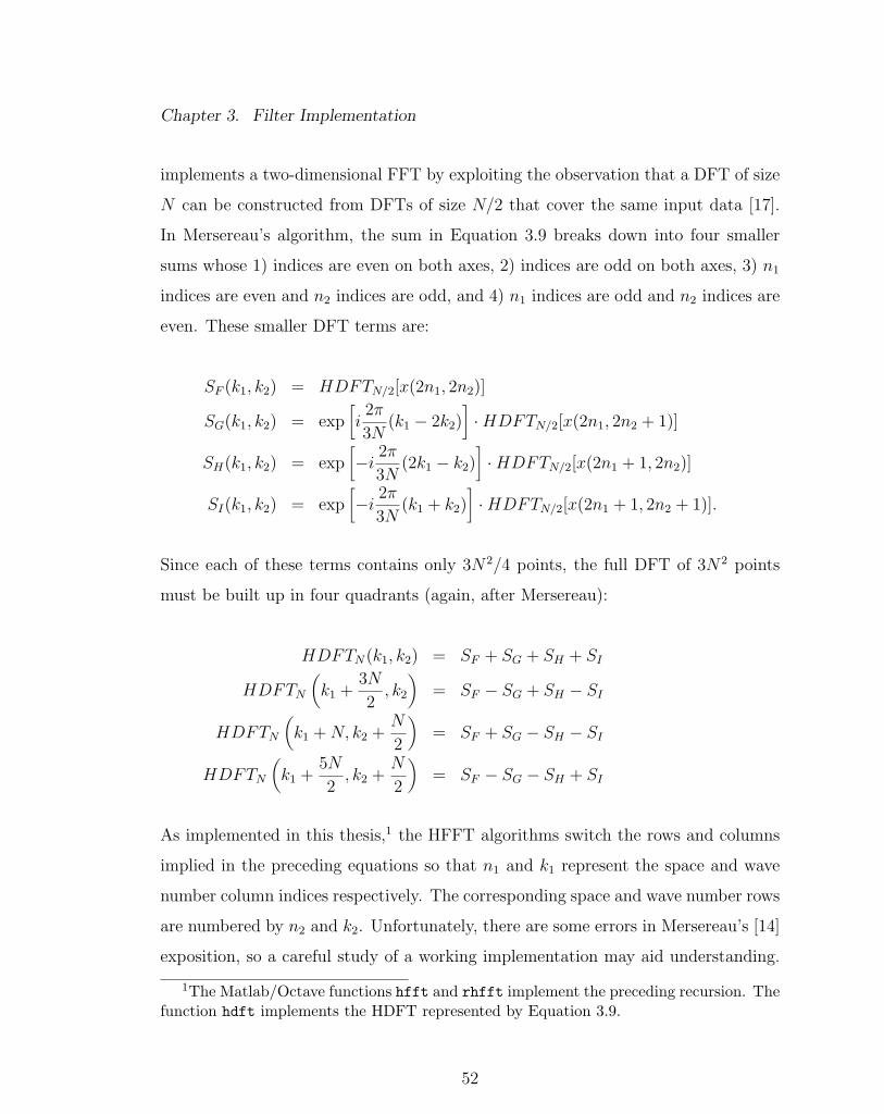
Chapter 3. Filter Implementation
implements a two-dimensional FFT by exploiting the observation that a DFT of size
N can be constructed from DFTs of size N/2 that cover the same input data [17].
In Mersereau’s algorithm, the sum in Equation 3.9 breaks down into four smaller
sums whose 1) indices are even on both axes, 2) indices are odd on both axes, 3) n1
indices are even and n2 indices are odd, and 4) n1 indices are odd and n2 indices are
even. These smaller DFT terms are:
SF (k1, k2) = HDFTN/2[x(2n1, 2n2)]
SG(k1, k2) = exp[i2π
3N(k1 − 2k2)
]·HDFTN/2[x(2n1, 2n2 + 1)]
SH(k1, k2) = exp[−i
2π
3N(2k1 − k2)
]·HDFTN/2[x(2n1 + 1, 2n2)]
SI(k1, k2) = exp[−i
2π
3N(k1 + k2)
]·HDFTN/2[x(2n1 + 1, 2n2 + 1)].
Since each of these terms contains only 3N2/4 points, the full DFT of 3N2 points
must be built up in four quadrants (again, after Mersereau):
HDFTN(k1, k2) = SF + SG + SH + SI
HDFTN
(k1 +
3N
2, k2
)= SF − SG + SH − SI
HDFTN
(k1 + N, k2 +
N
2
)= SF + SG − SH − SI
HDFTN
(k1 +
5N
2, k2 +
N
2
)= SF − SG − SH + SI
As implemented in this thesis,1 the HFFT algorithms switch the rows and columns
implied in the preceding equations so that n1 and k1 represent the space and wave
number column indices respectively. The corresponding space and wave number rows
are numbered by n2 and k2. Unfortunately, there are some errors in Mersereau’s [14]
exposition, so a careful study of a working implementation may aid understanding.
1The Matlab/Octave functions hfft and rhfft implement the preceding recursion. Thefunction hdft implements the HDFT represented by Equation 3.9.
52

Chapter 3. Filter Implementation
See the Matlab/Octave Filter Code Appendix for listings of the HFFT algorithms.
Refer to Mersereau [14] for other details.
The HFFT implementation was written to run on Octave and, with only minor
modifications, should run under Matlab as well. The first argument is a matrix
containing a fundamental period of either an impulse response in the space domain
or a transfer function in the frequency domain. The second argument is the desired
size of the transform as the size N of the fundamental period. The last argument is
either 1 if a forward transform from space to frequency domain is desired or -1 for
the reverse direction. The normalizing factor in the reverse direction is 1/3N2 and
must be supplied by the user.
3.3.5 McClellan Frequency Transformation
Designing accurate filters for a pyramid decomposition can be difficult and time-
consuming. If existing filters suit a particular application, then it is often advisable
to use them. In the case of the standard shiftable pyramid presented by Karasiridis
and Simoncelli [10], filter kernels are provided. Since the filter tap values are sampled
on a rectangular grid, reusing the filters requires constructing corresponding filters on
a hexagonal grid. One obvious approach is to resample the kernels themselves with
the appropriate interpolation function. Our attempts to use this approach failed.
The Fourier transform offers itself as the ideal interpolation function, whereby the
kernel transforms into it complementary function in the frequency domain and is
resampled there. This subsection discusses that approach.
The McClellan frequency transformation method transforms a one-dimensional
linear phase FIR filter into a two-dimensional filter with similar properties. The
impulse response h(n) of a linear phase FIR filter is symmetrical about the center
53

Chapter 3. Filter Implementation
tap, so that the transfer function is
H(ω) =N∑
n=−N
h(n) exp(−iωn)
= h(0) +N∑
n=1
2h(n) cos(ωn)
=N∑
n=0
a(n) cos(ωn). (3.10)
A one-dimensional FIR filter with a given number of taps can be transformed into
a two-dimensional filter by replacing the cos(ωn) factor in each term by a transformed
function expressing the frequency in two dimensions. This transformed function
must be a sum of cosine functions so that the two-dimensional transfer function
can have the same number of terms in its Fourier expansion as the original one-
dimensional transfer function. To see this, consider that the transfer function sum
can be expressed as the sum of powers of the cosine, since cos(ωn) can be expressed
as the Chebyshev polynomial of degree n. Thus,
H(ω) =N∑
n=0
b(n)(cos(ω))n (3.11)
McClellan’s transformation substitutes a two-dimensional sum of cosines for cos(ω)
in the preceding equation. In particular [13, 14], consider the transformation
cos(ω) = fR(ω1, ω2)
= A + B cos(ω1) + C cos(ω2) + D cos (ω1 + ω2) + E cos (ω1 − ω2)
so that
H(ω1, ω2) =N∑
n=0
b(n)(fR(ω1, ω2))n
=N∑
n1=−N
N∑n2=−N
h(n1, n2) cos(n1ω1) cos(n2ω2),
54

Chapter 3. Filter Implementation
where h(n1, n2) = h(−n1,−n2), thereby causing terms containing sin(nω) to cancel
out.
Since the taps are symmetric about the center, the two-dimensional transfer func-
tion H(ω1, ω2) clearly corresponds to a linear-phase FIR filter. Moreover, the number
of distinct tap values is equal to the square of the number of taps required by the
prototype one-dimensional filter. The transformation produces a two-dimensional
filter with a transfer function that depends on the one-dimensional transfer function
in a way that is wholly determined by the transformation coefficients A, B, C, D,
and E. In general, these coefficients are found by imposing constraints on fR(ω1, ω2),
such as fR(0, 0) = 1, so that A+B +C +D +E = 1, and then optimizing the coeffi-
cients to minimize some error measure. It usually makes sense to use a known set of
coefficients that are tailored to the problem at hand. For hexagonal FIR filters with
circular symmetry, Mersereau suggests
cos ω = fH(ω1, ω2)
= A + B cos
(2ω1√
3
)+ C cos
(ω1√
3+ ω2
)+ D cos
(ω1√
3− ω2
),
where A = −13, B = C = D = 4
9.
To apply the transformation, pick ω1 and ω2, compute cos(ω) by calculating the
right hand side of the transformation, find ω by applying the cos−1 function to the
right hand side, and return the amplitude of the one-dimensional transfer function
at ω. The fqt Matlab/Octave function implements this procedure given ω1, ω2,
and the one-dimensional transfer function. The ftrans function computes the entire
two-dimensional transfer function, covering the hexagonal fundamental period. It
computes the ω1 and ω2 for each pair of hexagonal indices and calls fqt to perform
the McClellan transformation that computes the amplitude to insert at the indexed
location. Note that fqt scales the frequency by 34
so that the frequency is in the
same units as the rectangular-sampled transfer function from which it is sampled.
55
Chapter 3. Filter Implementation
By means of inverse HFFT, the two-dimensional transfer function transforms
into a set of approximately real-valued taps in the hexagonal (or affine) coordinate
system, since it is centered at the origin. To use the result with the pyramid de-
composition software, a set of taps must be inserted into a rectangular coordinate
system with alternate offset rows. The file unhex Matlab/Octave function performs
this transformation and shifts the center of the new kernel to a predictable location
such that the entire kernel appears with positive indices. This array can be used
directly as a kernel in a convolution calculation. However, the kernel often contains
asymmetries that affect the accuracy of the filter it implements. These asymmetries
can be corrected by averaging tap values at the same distance from the center and us-
ing the averaged numbers instead. The radialize Matlab/Octave function converts
a kernel with such slight asymmetries into one that is perfectly circularly symmetric.
As will be shown in the next chapter, reconstruction errors can be reduced by this
method. In addition, some filters are actually improved by trimming the kernel to fit
entirely within a hexagon of a given size. The reader may apply the hexagonalize
Matlab/Octave function to a kernel if this is desired.
3.4 Oriented Filters
A steerable pyramid uses the responses of a small set of oriented basis filters at
fixed angle to synthesize an oriented filter at an arbitrary angle. The interpolation
functions that combine these basis filters depend only on the number of basis fil-
ters, which in turn depend on the order of the polynomial that is used to represent
the angular component of the basis filter transfer function [7]. The interpolation
functions are discussed in Chapter 2. This section discusses the computation of the
basis filters, whose transfer functions are products of an angular and a radial transfer
function [4, 7, 22].
56

Chapter 3. Filter Implementation
To compute an oriented basis filter by the direct analytical method, rewrite the
angular function as a cosine series, produce a radial kernel for each term, multiply
each radial kernel by its cosine function, and sum the resulting set of kernels weighted
by the cosine series coefficients to obtain the final kernel. Each basis function is
just a rotated copy of the unrotated basis function and so the oriented kernel can
be obtained by repeating the preceding steps for each basis filter using the cosine
function rotated by the same amount as the basis function.
Figure 3.7 shows a block diagram of the procedure for computing oriented kernels
using the analytical inverse Fourier transform. The so-called “Inverse k-th order
Hankel transform” in the diagram produces the radial k-th order term of the oriented
kernel from a one-dimensional transfer function, which is the radial component of
the oriented filter transfer function.
The direct method of computing the kernel by analytical inverse polar Fourier
transform enjoys the advantage that the desired kernel may be built up as the sum of
circularly symmetric kernels multiplied by cosine functions of the appropriate order.
That is, the angular function may be applied to the kernel in the space domain.
Because of this property, the accuracy of the oriented filter should be as good as
that of the radial filter from which it was derived. To militate against this benefit,
there is the fact that a k-th order angular term requires the k-th order bessel function
in the radial part of its Fourier transform.
hk(r) cos(kθ) = 4π(−i)k cos(kθ)∫ ∞
0RJk(2πrR)H(R)dR
h(r, θ) =N∑
k=0
hk(r) cos(kθ)
where H(R) is the radial transfer function of the filter. Figure 3.8 shows computed
radial kernels for k = 0, 1, and 3, where the angular function contains terms in eikθ
and the radial component of the transfer function is low-pass. Band-pass radial
57

Chapter 3. Filter Implementation
Figure 3.7: Procedure for constructing an oriented kernel by analytical inverse polarFourier transform.
transfer functions show a similar distribution of non-zero kernel values. The higher
the order k, the more non-zero terms are required to represent the filter to a given
accuracy. This problem is not specific to the direct computation method, but applies
to any computation of an oriented kernel. Complicated angular functions generally
require large kernels to implement them.
The alternative method of resampling in the frequency domain and inverse trans-
forming to obtain a kernel offers the possibility of a smaller kernel because the initial
radial kernel can be smaller. Nevertheless, the basic problem of kernel growth with
angular complexity remains. For a fixed kernel size, the reconstruction error will
grow with the order of the angular function. An additional source of error may re-
58

Chapter 3. Filter Implementation
Figure 3.8: Radial kernel profile as function of angular function order.
sult from the application of a DFT to a transfer function that is not band-limited.
This problem occurs with the standard shiftable pyramid band-pass filter, whose
transfer function does not fall to 0 at ω = π. Fortunately, each stage of the pyramid
is itself band limited, so that aliasing from band-pass filter errors should not result
in large reconstruction errors over and above those expected from kernel truncation.
To obtain an oriented filter kernel by frequency domain resampling, multiply a
circularly symmetric frequency response by the angular function and then obtain the
kernel by inverse Fourier transform. Figure 3.9 shows a diagram of the procedure
for constructing an oriented kernel on the hexagonal grid starting with an oriented
kernel on a rectangular grid. Of course, this procedure refers only to polar separable
filters, but there seems to be no need to deal with non-separable filters for this thesis.
Rotated basis kernels are obtained by inverse Fourier transforming the radial transfer
function multiplied by the rotated angular function. The Matlab/Octave Filter Code
59

Chapter 3. Filter Implementation
Figure 3.9: Procedure for constructing an oriented kernel by resampling method.
Appendix contains a set of routines that return a hexagonal oriented kernel given
a rectangular band-pass kernel. The functions bp0gen and bp1gen return the two
basis functions for the cos(θ) oriented filter given the circularly symmetric band-pass
kernel used in the circularly symmetric standard shiftable pyramid and found in the
spfilter.0 of the standard shiftable filter set [20]. The bp3gen function returns the
specified basis function for the cos3(θ) oriented filter given the 0 ◦ oriented band-pass
kernel found in spfilter.3 of the standard shiftable pyramid filter set [20].
60

Chapter 4
Pyramid Reconstruction Accuracy
Applications that employ multi-scale image analysis usually use a synthesis process
to recombine the pyramid subbands after they have been processed. The synthesis
process accurately reconstructs the input image if the subbands have not been al-
tered. For shiftable pyramids, it is sufficient that the power spectrum of the overall
pyramid transfer function be unity over the frequency range of interest. The trans-
fer function of internal stages may also exhibit this property, as with the standard
shiftable pyramid, or they may represent a system transfer function which is sub-
tracted from the original image at the start of analysis and then is recombined with
the difference to complete image synthesis, as in the original shiftable pyramid. In
either case, the accuracy of the synthesized image, which is reconstructed from the
pyramid subbands, depends on the accuracy with which each stage implements the
specified transfer function.
The filters used in the standard shiftable pyramid demonstrate a method of de-
signing filters for accurate reconstruction [10]. Accordingly, both the rectangular
and hexagonal filter sets provide very good reconstruction accuracy for the standard
shiftable pyramid transform. Hexagonal filters obtained by either direct analytical
61

Chapter 4. Pyramid Reconstruction Accuracy
computation or McClellan transformation exhibit the greatest accuracy for a partic-
ular kernel size.
The design of the filters used in the original shiftable pyramid [22] employed
a technique that neglected overall optimization of accuracy in favor of producing
kernels of manageable size. Partly as a result of this approach, the two low-pass
filters uniquely determine a band-pass filter transfer function that requires a large
convolution kernel to reproduce it accurately. Hexagonal kernels computed by either
method achieve greater accuracy with larger kernels.
The following sections present results for a range of kernel sizes, descriptions of
both pyramid designs, and descriptions of both filter construction methods. Recon-
struction accuracies for the circularly symmetric radial filters appear first, followed
by accuracy results for oriented filters of first order, i.e., based on cos(θ), and third
order, i.e., based on i cos3(θ). Finally, some accuracy measurements for steerable
transforms with three basis functions, i.e., based on cos2(θ)), and six basis functions,
i.e., based on i cos5(θ), are presented. It was our hope that these last transforms
would benefit from the higher symmetry of the hexagonal grid, but they were found
to display accuracies comparable to those of the other steerable transforms.
4.1 Accuracy of the Radial Filters
Reconstruction accuracy figures for the two quite dissimilar images shown in Fig-
ure 4.1 appear in the following tables. Both images consist of a 256 × 256 pixel
foreground approximately centered on a 512 × 512 pixel black background. This
embedding lessens edge effects of filtering for even very large (up to 41 × 41) ker-
nels for about 5 decomposition levels. The famous “lena” image downsampled to
256 × 256 pixels and then resampled with bilinear interpolation for the hexagonal
grid produced the results labeled “blena.” The column labeled “bdisk” contains
62

Chapter 4. Pyramid Reconstruction Accuracy
Figure 4.1: Images used for measuring reconstruction accuracy.
reconstruction accuracy results for a white disk on a black background.
The results reported here employ two measures for ascertaining reconstruction
accuracy. The first is the maximum absolute difference of pixel values between the
original image array and its reconstruction. The processing software converts the
original image, which is quantized to 256 levels, to a floating point array with values
that range from 0.0 to 1.0. Thus, the maximum difference value is normalized to a
fraction of full scale. The second measure is the variance about zero of the difference
between the original image and its reconstruction expressed in decibels.
Since a foreground image is embedded in a black background, it makes sense to
report variance and maximum difference of the foreground image by itself as well as
the same figures for the entire image. When errors for the full image are larger than
those for the foreground, this indicates that edge effects dominate. Figures for the
foreground image indicate the accuracy that can be expected when the embedding
technique is used to protect the image from edge effect errors. The benefit in recon-
63
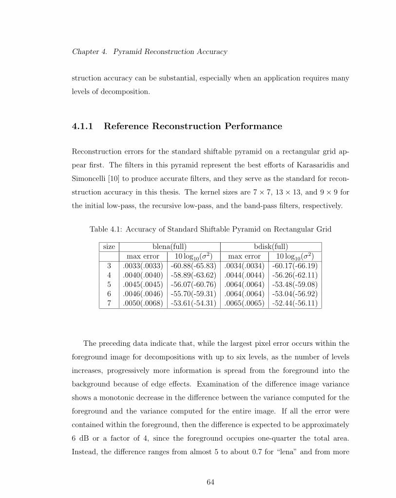
Chapter 4. Pyramid Reconstruction Accuracy
struction accuracy can be substantial, especially when an application requires many
levels of decomposition.
4.1.1 Reference Reconstruction Performance
Reconstruction errors for the standard shiftable pyramid on a rectangular grid ap-
pear first. The filters in this pyramid represent the best efforts of Karasaridis and
Simoncelli [10] to produce accurate filters, and they serve as the standard for recon-
struction accuracy in this thesis. The kernel sizes are 7 × 7, 13 × 13, and 9 × 9 for
the initial low-pass, the recursive low-pass, and the band-pass filters, respectively.
Table 4.1: Accuracy of Standard Shiftable Pyramid on Rectangular Grid
size blena(full) bdisk(full)max error 10 log10(σ
2) max error 10 log10(σ2)
3 .0033(.0033) -60.88(-65.83) .0034(.0034) -60.17(-66.19)4 .0040(.0040) -58.89(-63.62) .0044(.0044) -56.26(-62.11)5 .0045(.0045) -56.07(-60.76) .0064(.0064) -53.48(-59.08)6 .0046(.0046) -55.70(-59.31) .0064(.0064) -53.04(-56.92)7 .0050(.0068) -53.61(-54.31) .0065(.0065) -52.44(-56.11)
The preceding data indicate that, while the largest pixel error occurs within the
foreground image for decompositions with up to six levels, as the number of levels
increases, progressively more information is spread from the foreground into the
background because of edge effects. Examination of the difference image variance
shows a monotonic decrease in the difference between the variance computed for the
foreground and the variance computed for the entire image. If all the error were
contained within the foreground, then the difference is expected to be approximately
6 dB or a factor of 4, since the foreground occupies one-quarter the total area.
Instead, the difference ranges from almost 5 to about 0.7 for “lena” and from more
64

Chapter 4. Pyramid Reconstruction Accuracy
than 6 to about 3.7 for the “white disk.” The disparity between the images arises
from a larger background area surrounding the disk in the “white disk” image.
The decrease in variance difference between the full image and the foreground
image with the number of decomposition levels indicates spreading of information
from the foreground image to the background as the kernel size approaches that of
the image. Even with perfectly matched filters, the pyramid with not reconstruct the
image perfectly because of edge effects. Edge effects occur because the kernel extends
past the edges of the image for pixels near enough to the edge, and so arbitrary values
must substitute for actual values in this case. The convolution algorithm utilized here
uses a reflection scheme, where the pixels outside the image boundary reflect those
within the boundary as if in a mirror. This scheme produces reasonably good results,
but the best policy ensures that edge pixels matter as little as possible [5]. As the size
of the filtered image shrinks with each downsampling, the percentage of edge pixels
grows proportionately. At the seventh level of decomposition, the image is 8 × 8,
and every pixel is an edge pixel for the recursive low-pass filter, which is 13× 13. In
this case, the background area of “lena” contains the largest error. Performance for
“white disk” with seven decomposition levels looks surprisingly good.
4.1.2 Accuracy of the Original Shiftable Pyramid
In the original shiftable pyramid, two low-pass filters determine the transfer function
for the band-pass filter which determines the radial component of the oriented filters
used to achieve steerability. Evidently, a large kernel is necessary to produce an
accurate filter response at frequency ω = 0. Larger kernels produce greater accuracy
at zero frequency. Figure 4.2 shows the transfer functions of directly-computed
kernels together with the desired transfer function. The thirteen- and twenty-layer
kernels match the desired transfer function closely except for the region near zero
65

Chapter 4. Pyramid Reconstruction Accuracy
Figure 4.2: Band-pass responses for 7, 13, and 20 hexagonal kernel layers.
frequency. The seven-layer kernel produces an acceptable response (to within less
than one percent error in power) except near 0. The other two kernels match the
desired response to within 0.46 percent and 0.23 percent for the thirteen-layer and
twenty-layer kernels, respectively. The tabulated reconstruction accuracies following
reflect these observations.
The expression in the first column represents the filter type and the size of the
recursive low-pass L1, the initial low-pass L0, and the band-pass filter BP , respec-
tively. Names of hexagonal filters are of the form “tran(l1,l0,bp)” or “dir(l1,l0,bp),”
where the quantities in parentheses are the respective number of layers for the L1,
66

Chapter 4. Pyramid Reconstruction Accuracy
Table 4.2: Accuracy of Original Shiftable Pyramid with Analytical Filters
type(l1,l0,bp) size blena(full) bdisk(full)max error 10 log10(σ
2) max error 10 log10(σ2)
dir(4,6,7) 3 .051(.051) -29.78(-34.97) .084(.084) -28.23(-34.18)dir(4,6,7) 4 .074(.074) -27.66(-32.95) .11(.11) -26.59(-32.50)dir(4,6,7) 5 .080(.080) -26.79(-31.70) .10(.10) -26.81(-32.59)dir(4,6,7) 6 .099(.099) -26.85(-29.63) .10(.10) -26.87(-31.44)
dir(7,10,13) 3 .0082(.0082) -45.81(-50.97) .013(.013) -45.41(-51.22)dir(7,10,13) 4 .0086(.0086) -44.93(-49.66) .012(.012) -45.65(-51.17)dir(7,10,13) 5 .010(.038) -44.81(-44.68) .013(.013) -45.75(-50.28)dir(14,14,20) 3 .0042(.0042) -52.49(-57.51) .0044(.0044) -52.98(-58.60)dir(14,14,20) 4 .0039(.0047) -51.94(-56.01) .0041(.0041) -52.54(-57.80)dir(14,14,20) 5 .0070(.036) -49.50(-46.37) .0061(.011) -51.00(-53.89)
L0, and BP filters. The “tran” stands for a filter obtained by transformation, and
the “dir” notation means that the filter was calculated directly from the transfer
function using the analytical Fourier transform.
For a given kernel size, the directly-computed and McClellan transformation ker-
Table 4.3: Accuracy of Original Shiftable Pyramid with Transformed Filters
type(l1,l0,bp) size blena(full) bdisk(full)max error 10 log10(σ
2) max error 10 log10(σ2)
tran(4,6,7) 3 .062(.062) -29.20(-34.78) .087(.087) -27.97(-33.99)tran(4,6,7) 4 .076(.076) -27.31(-32.81) .10(.10) -26.46(-32.46)tran(4,6,7) 5 .082(.082) -26.60(-31.98) .093(.093) -26.88(-32.71)tran(4,6,7) 6 .084(.084) -26.80(-30.56) .094(.094) -27.18(-32.71)
tran(7,10,13) 3 .0077(.0077) -47.76(-52.82) .010(.010) -47.79(-53.61)tran(7,10,13) 4 .0076(.0076) -47.87(-52.13) .0086(.0086) -49.10(-54.31)tran(7,10,13) 5 .0063(.0065) -49.41(-51.11) .0062(.0062) -51.06(-53.59)tran(14,14,20) 3 .0037(.0037) -58.90(-62.28) .0033(.0033) -57.45(-62.81)tran(14,14,20) 4 .0026(.0026) -61.81(-61.19) .0032(.0032) -56.84(-60.94)tran(14,14,20) 5 .0036(.0077) -61.10(-55.30) .0036(.0059) -55.06(-55.89)
67

Chapter 4. Pyramid Reconstruction Accuracy
nels show comparable performance. As expected, the performance for “white disk”
consistently falls short of that for “lena” because of the poor band-pass performance
at 0 frequency. For sufficiently large kernels of either type, the accuracy of recon-
struction is comparable to or better than that of the carefully designed standard
shiftable pyramid with rectangular sampling. However, the large kernels produce
significant edge effect errors beyond a pyramid with four levels, and the computation
time required is likely to be unacceptable for most applications. In order to avoid
large kernels, it is necessary to use optimal design techniques. One-dimensional fil-
ters that satisfy design constraints imposed by the pyramid may be obtained by
optimization to achieve minimum reconstruction error. The standard shiftable pyra-
mid design utilizes filters that were designed with such a process and constructed on
a rectangular grid. These filters were reconstructed on a hexagonal grid and used to
produce the results reported in the next subsection.
4.1.3 Accuracy of the Standard Shiftable Pyramid
The standard shiftable pyramid uses filters carefully optimized for minimum recon-
struction error and for a particular kernel size. Excellent reconstruction accuracy is
obtained with a relatively small kernel size for both types of filter. Tabulated results
follow.
The quality of the filter match shows up immediately in the results for the small-
est kernel, in which the maximum pixel error is approximately one quarter the error
for the filters in the original shiftable pyramid. As might be expected, filters con-
structed by resampling kernels which have been optimized for a particular set of
sizes perform best with similar kernel sizes. Measurements indicate that the filter
accuracy actually degrades when the kernel size of the anti-aliasing low-pass filter is
above a particular optimum value. This phenomenon might be attributed to noise
68

Chapter 4. Pyramid Reconstruction Accuracy
Table 4.4: Accuracy of Standard Shiftable Pyramid with Analytical Filters
type(l1,l0,bp) size blena(full) bdisk(full)max error 10 log10(σ
2) max error 10 log10(σ2)
dir(4,6,7) 3 .013(.013) -50.69(-54.95) .013(.013) -50.75(-55.80)dir(4,6,7) 4 .015(.015) -47.89(-51.86) .015(.015) -46.78(-51.85)dir(4,6,7) 5 .017(.017) -46.04(-49.07) .020(.020) -43.20(-48.12)dir(4,6,7) 6 .018(.018) -44.96(-46.54) .022(.023) -41.04(-44.82)dir(4,6,7) 7 .017(.024) -44.11(-44.13) .024(.024) -38.96(-42.70)
dir(7,10,13) 3 .0039(.0039) -61.09(-65.00) .0044(.0044) -60.49(-65.80)dir(7,10,13) 4 .0049(.0049) -58.61(-61.90) .0050(.0050) -57.00(-62.01)dir(7,10,13) 5 .0051(.0051) -56.67(-58.92) .0061(.0061) -55.62(-58.82)dir(7,10,13) 6 .0055(.0078) -56.64(-56.74) .0061(.0086) -52.81(-53.61)dir(7,10,13) 7 .0073(.013) -52.93(-51.38) .0081(.011) -49.19(-49.77)dir(14,14,20) 3 .0041(.0041) -60.85(-64.94) .0042(.0042) -59.54(-65.11)dir(14,14,20) 4 .0043(.0043) -58.92(-62.33) .0053(.0053) -55.67(-60.99)dir(14,14,20) 5 .0054(.0054) -56.17(-58.81) .0063(.0063) -53.66(-58.22)dir(14,14,20) 6 .0063(.0081) -54.79(-56.44) .0092(.0092) -50.26(-52.57)
in the kernel generation process, or it might be that the desired filter response is
achieved optimally at a particular kernel size. This thesis does not try to resolve this
issue.
Both types of filter have an optimum kernel size for which they have comparable
levels of performance. Moreover, the best results exceed the performance of the
rectangular filter used as a standard. This demonstrates that a good design can
be copied accurately from one sampling system to another. It is interesting that
the McClellan transformation filter outperforms the analytically constructed filter.
This disparity may be attributed to the fact that the analytically constructed filter
tries to copy a slightly incorrect filter (and does so precisely), while the McClellan
transformation mirrors the process that produced the original filter, thus reproducing
the optimized two-dimensional transfer function more accurately.
69

Chapter 4. Pyramid Reconstruction Accuracy
Table 4.5: Accuracy of Standard Shiftable Pyramid with Transformed Filters
type(l1,l0,bp) size blena(full) bdisk(full)max error 10 log10(σ
2) max error 10 log10(σ2)
tran(4,7,7) 3 .0095(.0095) -53.21(-57.60) .0074(.0074) -53.15(-58.55)tran(4,7,7) 4 .011(.011) -50.12(-54.38) .0093(.0093) -48.91(-54.38)tran(4,7,7) 5 .013(.013) -47.74(-51.80) .013(.013) -45.65(-51.15)tran(4,7,7) 6 .013(.013) -46.45(-49.73) .017(.017) -42.38(-47.79)tran(4,7,7) 7 .013(.014) -45.24(-45.88) .023(.023) -40.15(-44.67)tran(7,8,13) 3 .0022(.0022) -65.12(-69.00) .0020(.0020) -65.02(-70.39)tran(7,8,13) 4 .0042(.0042) -62.89(-66.41) .0065(.0065) -61.10(-66.18)tran(7,8,13) 5 .0036(.0036) -60.83(-63.75) .0038(.0038) -60.82(-64.46)tran(7,8,13) 6 .0036(.0067) -60.22(-59.59) .0046(.0046) -59.03(-58.68)tran(7,8,13) 7 .0036(.0011) -59.86(-49.63) .0076(.0084) -54.18(-51.57)tran(7,10,13) 3 .012(.012) -48.95(-53.34) .0098(.0098) -48.70(-54.22)tran(7,10,13) 4 .014(.014) -46.51(-50.62) .013(.013) -44.60(-50.19)tran(7,10,13) 5 .016(.016) -44.28(-48.29) .018(.018) -40.87(-46.47)tran(7,10,13) 6 .017(.017) -42.41(-45.97) .023(.023) -38.68(-44.27)tran(7,10,13) 7 .018(.018) -41.72(-43.93) .026(.026) -37.72(-42.93)tran(14,14,20) 3 .012(.012) -48.24(-52.57) .011(.011) -47.44(-52.99)tran(14,14,20) 4 .014(.015) -46.02(-49.99) .014(.014) -43.19(-48.80)tran(14,14,20) 5 .016(.016) -43.48(-47.46) .021(.021) -40.04(-45.64)tran(14,14,20) 6 .017(.017) -42.15(-45.77) .026(.026) -38.28(-43.55)tran(14,8,20) 3 .0022(.0022) -65.14(-69.07) .0019(.0019) -64.94(-70.34)tran(14,8,20) 4 .0032(.0032) -63.25(-67.05) .0062(.0062) -61.28(-66.36)tran(14,8,20) 5 .0033(.0033) -62.20(-64.92) .0039(.0039) -60.48(-64.21)tran(14,8,20) 6 .0032(.0060) -60.50(-60.32) .0032(.0038) -61.04(-59.78)
4.2 Accuracy of the Oriented Filters
The reconstruction accuracy of an oriented filter for a given kernel size is generally
expected to be lower than for the circularly symmetric filter from which it is derived.
The highest order of the Bessel function in the polar Fourier transform equals the
highest order term of the Fourier expansion of the angular function embodied in the
oriented filter. As noted in Chapter 3 and depicted in Figure 3.8, the higher the order
of the Bessel function, the more extended the support required for the transformed
70

Chapter 4. Pyramid Reconstruction Accuracy
transfer function in the space domain. The reconstruction accuracy results for the
rectangular filters for the standard shiftable pyramid support this expectation.
4.2.1 Rectangular Standard Shiftable Pyramid Accuracy
The rectangular filter kernels are 9 × 9, 17 × 17, and 9 × 9 for the initial low-pass,
recursive low-pass, and oriented band-pass filter kernels, respectively.
Table 4.6: Accuracy of Rectangular Standard Shiftable Pyramid with cos(θ)
size blena(full) bdisk(full)max error 10 log10(σ
2) max error 10 log10(σ2)
3 .016(.016) -49.15(-54.29) .014(.014) -49.52(-55.54)4 .018(.018) -47.36(-52.16) .029(.029) -46.30(-52.02)5 .020(.038) -46.22(-45.32) .024(.024) -41.86(-27.26)6 .022(.065) -42.91(-35.27) .025(.045) -41.22(-37.59)7 .12(.24) -25.78(-23.18) .092(.164) -28.062(-25.51)
Table 4.7: Accuracy of Rectangular Standard Shiftable Pyramid with cos3(θ)
size blena(full) bdisk(full)max error 10 log10(σ
2) max error 10 log10(σ2)
3 .020(.020) -47.37(-52.47) .016(.016) -47.70(-53.72)4 .025(.025) -45.32(-50.08) .029(.029) -44.33(-50.07)5 .028(.038) -43.54(-44.39) .029(.029) -40.16(-45.50)6 .033(.070) -40.98(-35.34) .034(.044) -39.41(-37.61)7 .12(.23) -26.38(-23.30) .094(.17) -28.85(-25.05)
The results show that the error of the oriented filters is approximately five times
the error for the purely radial filters, and the error of the third order filter is compa-
rable. These figures are close to the reconstruction errors reported in Karasaridis and
Simoncelli [10]. The first order filter had reconstruction accuracy of -44.36 dB(-50.29
71

Chapter 4. Pyramid Reconstruction Accuracy
dB) variance for the cropped (full) zone plate image and a pyramid with three levels.
Karasaridis and Simoncelli reported -47 dB variance for a similar zone plate image
and pyramid. The third order filter produced a three-level reconstruction error of
−41.38 dB(-47.33 dB) for the same image, and the paper claims ≈ -40 dB. These
figures correspond to respective standard deviations of the error about 0 of .0045 and
.01, respectively. The quantization is .0039 for the 256 grey level images used here,
so these errors correspond to between about 1 and 2.5 shades of gray.
4.2.2 Steerable Original Shiftable Pyramid Accuracy
The reconstruction accuracy for the steerable original shiftable pyramid is much
higher than expected. The readiest explanation for this behavior is that the greatest
source of filter error lies near frequency zero in the radial component. The oriented
filters force the DC component of the transfer function to zero, thus producing an
extremely accurate band-pass filter. The results shown in the following table report
maximum reconstruction error for the first order, i.e. based on cos(θ), oriented filter
less than one-tenth the maximum error for the circularly symmetric filter from which
it was derived.
This phenomenon occurs only for the analytically computed filter kernels, which
compute an exact impulse response from an exact transfer function. Kernels com-
puted by the McClellan transformation and inverse HFFT produce more typical ac-
curacies. The McClellan transformation produces an approximately circular transfer
function which is then multiplied by the angular function. Errors attributable to
approximation may explain the lower reconstruction accuracy of filters constructed
by this method.
72

Chapter 4. Pyramid Reconstruction Accuracy
Table 4.8: Accuracy of Original Shiftable Steerable Pyramid with cos(θ)
type(l1,l0,bp) size blena(full) bdisk(full)max error 10 log10(σ
2) max error 10 log10(σ2)
dir(7,10,13) 3 .0007(.0008) -75.34(-78.87) .0007(.0007) -74.07(-79.10)dir(7,10,13) 4 .0007(.0030) -73.78(-67.96) .0009(.0047) -71.84(-70.23)dir(7,10,13) 5 .0028(.095) -61.70(-40.26) .0026(.013) -64.53(-54.95)dir(7,10,13) 6 .0094(.32) -47.94(-25.92) .0096(.17) -47.86(-32.09)tran(7,10,13) 3 .011(.011) -50.59(-55.43) .012(.012) -49.11(-54.91)tran(7,10,13) 4 .014(.014) -48.72(-53.03) .016(.016) -46.59(-51.98)tran(7,10,13) 5 .015(.11) -46.60(-38.31) .020(.020) -43.37(-47.69)tran(7,10,13) 6 .018(.31) -42.68(-25.87) .024(.19) -40.13(-30.46)
4.2.3 Hexagonal Standard Shiftable Pyramid Accuracy
The filters computed for the standard shiftable pyramid exhibit accuracy comparable
to that of the same pyramid on the rectangular grid, although larger kernels are
necessary to achieve this result. The filter set provided by Simoncelli [20] for the
first order oriented pyramid produced poor reconstruction accuracy on a hexagonal
grid. We used the circularly symmetric filters instead, i.e., the filters used in the
design of the radial components of the filters, with kernel sizes identical to those
that produced the best performance for the circularly symmetric pyramid. The
third order filters provided by Simoncelli worked well. Directly computed kernels
performed comparably to kernels computed by McClellan transformation.
The third order filters perform about as well as the first order filters, despite the
expected broadening of the impulse response due to the higher order Bessel functions
in the transform integral. This good performance may be attributed to painstaking
optimization for minimum reconstruction error when designing each set of filters.
73

Chapter 4. Pyramid Reconstruction Accuracy
Table 4.9: Accuracy of Original Shiftable Oriented Pyramid with cos3(θ)
type(l1,l0,bp) size blena(full) bdisk(full)max error 10 log10(σ
2) max error 10 log10(σ2)
dir(4,6,7) 3 .013(.013) -49.59(-53.28) .012(.012) -48.64(-53.80)dir(4,6,7) 4 .015(.015) -47.88(-51.52) .028(.028) -45.64(-50.42)dir(4,6,7) 5 .017(.092) -47.63(-40.07) .017(.017) -44.39(-47.97)dir(4,6,7) 6 .021(.31) -43.37(-25.94) .020(.18) -42.53(-31.80)
dir(7,10,13) 3 .0035(.0035) -57.56(-63.61) .0034(.0034) -57.93(-63.54)dir(7,10,13) 4 .0042(.0043) -58.06(-60.52) .0047(.0047) -53.53(-58.96)dir(7,10,13) 5 .0059(.090) -52.46(-40.22) .0060(.0072) -51.41(-53.41)dir(7,10,13) 6 .014(.30) -45.51(-26.20) .013(.18) -45.64(-31.95)tran(7,10,13) 3 .014(.014) -48.78(-53.41) .016(.016) -46.50(-52.34)tran(7,10,13) 4 .016(.016) -46.43(-50.81) .018(.018) -43.11(-48.82)tran(7,10,13) 5 .017(.11) -43.16(-38.12) .022(.022) -40.06(-45.09)tran(7,10,13) 6 .021(.30) -40.02(-26.13) .027(.20) -37.84(-30.35)
4.2.4 Additional Oriented Filters for the Original Shiftable
Pyramid
The oriented filter sets presented in the preceding sections align on symmetry axes of
the square sampling grid. Even though the 45 degree axis aligns with fewer samples
than the horizontal and vertical axes do, this does not detectably affect performance.
Since the pyramid is oversampled, this is to be expected. The hexagonally sampled
filters perform as well as the rectangularly sampled filters for the same reason.
The last two oriented filters presented in the following examine the reconstruction
accuracy obtained with filters whose basis components align along the axes of a
hexagonal grid. The cos2(θ) filter is constructed with three basis filters aligned to
0 ◦, 60 ◦, and 120 ◦, while the cos5(θ) filter has basis filters aligned to 0 ◦, 30 ◦, 60 ◦,
90 ◦, 120 ◦, and 150 ◦. Figure 4.3 shows the “lena” image after filtering with the
three cos2(θ) basis filters. Hexagonal renderings of the corresponding kernels appear
below each filtered image. Figure 4.4 similarly shows the same image filtered with
74

Chapter 4. Pyramid Reconstruction Accuracy
Table 4.10: Accuracy of Oriented Shiftable Pyramid with cos(θ)
type(l1,l0,bp) size blena(full) bdisk(full)max error 10 log10(σ
2) max error 10 log10(σ2)
dir(4,6,7) 3 .035(.035) -41.41(-45.85) .028(.028) -42.11(-47.59)dir(4,6,7) 4 .041(.041) -38.92(-43.20) .035(.035) -38.40(-43.87)dir(4,6,7) 5 .045(.048) -37.17(-40.98) .031(.042) -34.20(-39.50)dir(4,6,7) 6 .062(.26) -32.93(-27.89) .069(.069) -31.10(-35.30)
dir(7,10,13) 3 .016(.016) -50.04(-53.73) .012(.012) -50.71(-55.90)dir(7,10,13) 4 .021(.021) -47.49(-50.79) .027(.027) -47.57(-52.17)dir(7,10,13) 5 .019(.024) -46.44(-47.42) .026(.029) -46.21(-47.52)dir(7,10,13) 6 .028(.25) -41.05(-28.47) .030(.060) -41.75(-38.30)dir(7,10,13) 7 .049(.39) -31.44(-20.60) .065(.35) -32.79(-21.54)tran(7,8,13) 3 .022(.022) -47.10(-51.03) .016(.016) -47.67(-53.18)tran(7,8,13) 4 .022(.023) -44.70(-47.92) .021(.021) -44.50(-49.51)tran(7,8,13) 5 .025(.029) -43.09(-44.94) .023(.039) -43.34(-44.88)tran(7,8,13) 6 .037(.25) -41.25(-28.54) .039(.089) -40.86(-35.40)tran(7,8,13) 7 .057(.37) -32.12(-20.52) .078(.32) -32.33(-21.60)
the six cos5(θ) basis filters and the corresponding six filter kernels. The orientation
directions should be apparent from both the kernels and the image features that are
accentuated in a given image. Each filter emphasizes the intensity gradient, so that
features aligned along the filter orientation disappear and those perpendicular to it
are enhanced.
The following tables contain reconstruction accuracy results for the third order
and sixth order oriented filters. The cos2(θ) filter performs respectably, but not as
well as the cos3(θ) filter. This disappointing result can possibly be attributed to the
zero frequency term in the cos2(θ) = 12(1 + 2 cos(2θ)) function, which has no angular
function to pin its transfer function to zero at ω = 0. The cos5(θ) filter performs
comparably well, but its accuracy falls off rapidly with the number of levels because
of its high angular order. The improved three level performance of the cos5(θ) filter
with twenty layers indicates that accuracy improves further with kernel size.
75

Chapter 4. Pyramid Reconstruction Accuracy
Table 4.11: Accuracy of Oriented Standard Shiftable Pyramid with cos3(θ)
type(l1,l0,bp) size blena(full) bdisk(full)max error 10 log10(σ
2) max error 10 log10(σ2)
dir(7,10,13) 3 .019(.019) -47.60(-51.48) .013(.013) -47.49(-52.91)dir(7,10,13) 4 .025(.033) -45.98(-47.89) .034(.034) -44.30(-49.45)dir(7,10,13) 5 .024(.081) -44.64(-40.07) .026(.042) -41.94(-43.47)dir(7,10,13) 6 .037(.23) -40.43(-28.41) .046(.099) -42.23(-32.37)dir(7,10,13) 7 .11(.41) -27.10(-21.06) .10(.43) -27.57(-20.91)tran(7,11,13) 3 .020(.020) -47.44(-51.47) .014(.014) -47.94(-53.38)tran(7,11,13) 4 .023(.033) -45.34(-47.40) .030(.030) -45.73(-50.59)tran(7,11,13) 5 .026(.075) -44.83(-39.92) .036(.036) -45.11(-44.95)tran(7,11,13) 6 .037(.23) -40.39(-28.52) .059(.099) -40.36(-32.10)tran(7,11,13) 7 .091(.38) -26.26(-28.82) .094(.38) -27.63(-21.17)
The standard shiftable pyramid does not supply third and sixth order angular
functions, so it was not possible to obtain results for these filters.
Table 4.12: Accuracy of Original Shiftable Oriented Pyramid with cos2(θ)
type(l1,l0,bp) size blena(full) bdisk(full)max error 10 log10(σ
2) max error 10 log10(σ2)
dir(7,10,13) 3 .0087(.0087) -48.78(-53.58) .0079(.0079) -50.76(-55.93)dir(7,10,13) 4 .0078(.0085) -49.31(-52.41) .0056(.0056) -52.25(-55.71)dir(7,10,13) 5 .0094(.066) -50.79(-42.36) .0048(.014) -55.10(-52.11)dir(7,10,13) 6 .017(.12) -44.89(-33.93) .014(.14) -45.18(-33.29)
76

Chapter 4. Pyramid Reconstruction Accuracy
Figure 4.3: “lena” image convolved with three cos2(θ) basis kernels.
Table 4.13: Accuracy of Original Shiftable Oriented Pyramid with cos5(θ)
type(l1,l0,bp) size blena(full) bdisk(full)max error 10 log10(σ
2) max error 10 log10(σ2)
dir(7,10,13) 3 .0082(.0082) -51.64(-55.84) .0078(.0078) -50.44(-56.03)dir(7,10,13) 4 .010(.010) -50.02(-53.29) .0096(.0096) -46.12(-51.63)dir(7,10,13) 5 .012(.086) -46.16(-39.76) .014(.014) -43.75(-46.94)dir(7,10,13) 6 .020(.29) -41.65(-26.41) .021(.19) -41.35(-31.41)dir(7,10,20) 3 .0033(.0034) -60.37(-63.73) .0045(.0045) -57.38(-62.83)dir(7,10,20) 4 .0043(.012) -56.90(-57.54) .0050(.0050) -53.69(-57.78)dir(7,10,20) 5 .0063(.086) -53.97(-40.17) .0056(.014) -52.87(-48.05)dir(7,10,20) 6 .013(.29) -46.47(-26.46) .013(.019) -46.35(-31.39)
77

Chapter 4. Pyramid Reconstruction Accuracy
Figure 4.4: “lena” image convolved with six cos5(θ) basis kernels.
78

Chapter 5
Noise Reduction Using Local
Orientation Analysis
5.1 Application Overview
This final chapter presents an application that attempts to take advantage of the
higher orientation accuracy of the hexagonal steerable pyramid when compared to
its rectangularly sampled counterpart. Because of its higher angular resolution, any
measurement of local orientation by a hexagonal oriented filter should produce a
more accurate signal than is produced by a rectangular oriented filter with the same
sampling interval. The following discussion first presents comparative results of local
orientation mapping [22] for a “cross” figure and for the “lena” image.
No practical difference in the properties of the orientation map are observed
between hexagonal and rectangular pyramids. It is perhaps due to this fact that
a noise reduction application using local orientation analysis [22] does not perform
significantly better with hexagonal sampling than it does with rectangular sampling.
These results are unexpected and somewhat disappointing, but we expect that a
79

Chapter 5. Noise Reduction Using Local Orientation Analysis
more carefully chosen application or an implementation of this application with wider
bandwidth images would demonstrate the higher angular resolution of the hexagonal
grid. We report the methods used to implement the application and discuss local
orientation analysis in order to support future work.
As described in Simoncelli et al [22], removal of noise depends on detecting some
property of the noise that differs from the same property of the image. The local
orientation of image features should be much higher than that of the noise, so mea-
surements of local orientation energy can be used to remove noise from an image.
Oriented features may include both lines and edges, which require even and odd sym-
metry filters, respectively, for their detection. A quadrature pair of filters provides
both symmetries. The derivation and use of these filter pairs will be presented.
5.2 Local Orientation Mapping
This section presents a comparison between the results of a measurement process
for an image represented using a square grid and results of the same process on an
image represented using a hexagonal grid. Since the measurements are very likely
dependent on the specific sampling process, it is important to take sample density into
account. In this section and in the following section, which describes the application
of local orientation analysis to noise reduction, the two images have nearly identical
sample density. They are derived from a 512 × 512 image which is filtered by a
Gaussian and then downsampled. For the square sampled image, the samples are
taken every other point in both horizontal and vertical directions so that a square
grid results. For the hexagonal image, the sample points are decimated by the same
ratio, but alternate rows are shifted one sample over to produce a stretched hexagonal
grid. That is, the grid has vertical spacing that is 2/√
3 larger than for a regular
hexagonal grid. This distortion should not make any difference in measurement
80

Chapter 5. Noise Reduction Using Local Orientation Analysis
accuracy and leaves the two sample grids with nearly the same density. Figure 5.1
shows the two downsampling patterns used. We anticipate that the advantage of
Figure 5.1: Square and hexagonal downsampling patterns for noise reduction com-parison.
a regular hexagonal sampling grid lies with its higher sample density for the same
sample spacing, but resampling the image with this spacing is difficult to do without
inadvertantly filtering the image, i.e., during interpolation, or otherwise introducing
errors, i.e., through aliasing, to the image. Therefore, we will leave exploration of
this issue to future work and present results obtained with rectangular and hexagonal
images having nearly equal spacing.
Measurements of extent, location, and orientation characterize an image feature
sufficiently for many image processing applications. Some applications, such as noise
removal, can effectively utilize orientation information alone, since it is only necessary
to determine the degree to which an area of the image is oriented or non-oriented
to decide whether or not it is noise. The accuracy of the orientation measurement
determines the accuracy with which image features that remain after noise removal
are represented, so that a filter that delivers a more accurate orientation signal should
reproduce the original image with smaller errors.
A typical oriented filter computes a directional derivative on pixel grey values.
81

Chapter 5. Noise Reduction Using Local Orientation Analysis
In the frequency domain, this is equivalent to multiplying the Fourier transform of
the image by the transfer function of a band pass filter multiplied by cosk(θ − θi),
where k is the integral degree of the derivative, θ is the angular variable, and θi is the
dominant direction of the angular function. Consider the case where θi = 0. For odd
k, cosk(θ) is positive over the entire right half of the frequency plane and negative
over the entire left half of the plane. For even k, cosk(θ) is positive over the entire
plane. The Hilbert transform of a filter kernel yields its quadrature counterpart
[3], and the Fourier transform of the Hilbert transform of the kernel produces a
transfer function which is identical to the transfer function of the original filter but
which is multiplied by -1 over half the frequency plane [3]. The line that divides the
frequency plane into two halves passes through the origin, and it is perpendicular to
the dominant direction of the transfer function of the original filter [11]. Figure 5.2
shows the 0 ◦ basis kernel for the cos5(θ) oriented filter on the left. The kernel on the
right side of the figure is its quadrature counterpart. The kernel on the right clearly
displays symmetry from left to right, while the kernel on the left does not. In fact,
the lefthand kernel is anti-symmetric from left to right.
Figure 5.2: 0 ◦ basis kernel for cos5(θ) oriented filter and its quadrature counterpart.
82

Chapter 5. Noise Reduction Using Local Orientation Analysis
To measure the orientation strength and dominant orientation angle at any point
in the image, it is necessary to filter the image with both the oriented filter and
its quadrature counterpart. This procedure produces an odd symmetric filter from
an even symmetric filter, and vice versa. Mathematically speaking, the quadrature
filter is the analytical completion of the original filter [3], so that the pair represents
the full complex filter.
An orientation mapping plots the orientation energy at a particular image point
as a function of steering angle. Energy is measured by steering the filter and its
quadrature counterpart to a given angle and then summing the squares of the pixel
amplitudes from both filters [22]. To get the pixel amplitude for the filtered image,
it is necessary only to sum the products of the amplitude with each kernel element
for the oriented filter and normalize. The anti-aliasing low-pass pyramid filter serves
as the normalization standard, so the sum of its kernel elements provides the nor-
malization constant.
The steerable filter used in the following for local orientation analysis is based
on cos5(θ). The angular function for the quadrature filter is therefore | cos5(θ)|.
The simplest way to compute a kernel for the quadrature filter is to determine the
first few coefficients of the Fourier series for the angular function and then directly
compute each term of the kernel as described in Section 3.2 [7]. The Fourier seriers
is computed using Matlab/Octave. The dot product of the sampled angular function
and the sampled cosine function of the desired frequency gives the raw coefficient for
that frequency. The normalized coefficient for a particular frequency is obtained by
dividing the raw coefficient by N/2, where N is the number of samples. Dividing the
DC coefficient by 2 again yields the normalized coefficient for frequency zero. The
quadrature function in this case is even, so that only even frequencies in the cosine
series have nonzero coefficients. The pyramid software divides the coefficients by
2q−1, where q is the maximum frequency in the Fourier series expansion. Therefore,
83
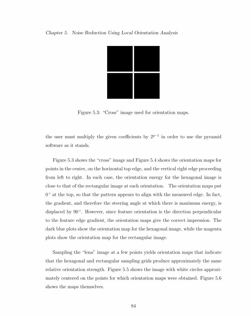
Chapter 5. Noise Reduction Using Local Orientation Analysis
Figure 5.3: “Cross” image used for orientation maps.
the user must multiply the given coefficients by 2q−1 in order to use the pyramid
software as it stands.
Figure 5.3 shows the “cross” image and Figure 5.4 shows the orientation maps for
points in the center, on the horizontal top edge, and the vertical right edge proceeding
from left to right. In each case, the orientation energy for the hexagonal image is
close to that of the rectangular image at each orientation. The orientation maps put
0 ◦ at the top, so that the pattern appears to align with the measured edge. In fact,
the gradient, and therefore the steering angle at which there is maximum energy, is
displaced by 90 ◦. However, since feature orientation is the direction perpendicular
to the feature edge gradient, the orientation maps give the correct impression. The
dark blue plots show the orientation map for the hexagonal image, while the magenta
plots show the orientation map for the rectangular image.
Sampling the “lena” image at a few points yields orientation maps that indicate
that the hexagonal and rectangular sampling grids produce approximately the same
relative orientation strength. Figure 5.5 shows the image with white circles approxi-
mately centered on the points for which orientation maps were obtained. Figure 5.6
shows the maps themselves.
84

Chapter 5. Noise Reduction Using Local Orientation Analysis
Figure 5.4: Orientation maps at center, upper horizontal edge, right vertical edge ofthe cross.
Comparison of the hexagonal and rectangular orientation maps indicate that the
strength of the orientation signal for hexagonal images is about the same as that for
rectangular images.
85

Chapter 5. Noise Reduction Using Local Orientation Analysis
Figure 5.5: Locations of orientation mapping points for “lena.”
86

Chapter 5. Noise Reduction Using Local Orientation Analysis
Figure 5.6: Orientation maps at various points of “lena” image.
87

Chapter 5. Noise Reduction Using Local Orientation Analysis
5.3 Noise Reduction Application
Random pixel noise can produce image features with multi-pixel extent and orien-
tation but only with small probability. True image features must extend over finite
areas and have edges with measurable orientation. Therefore, noise can be distin-
guished from image features by measuring local orientation energy. This is computed
as the sum of the squares of the pixel amplitudes from the image as filtered by an
oriented filter and its quadrature counterpart. Figure 5.7 shows the noise procedure
described in the Simoncelli, et al paper [22].
Figure 5.7: Noise reduction by local orientation analysis.
The pyramid transform described in Simoncelli, et al [22] supports local orien-
tation analysis by decomposing the input image into a high-pass component and
88

Chapter 5. Noise Reduction Using Local Orientation Analysis
a low-pass component, and then filtering the low-pass component with a steerable
oriented filter. A steerable pyramid using filters with odd symmetry and another
steerable pyramid using the corresponding quadrature partners with even symmetry
suffice to support local orientation analysis of any input image. Freeman and Adel-
son [7] describe a method for rapid approximation of the local orientation energy and
dominant direction of every point in an image. If G(θ) and H(θ) are respectively
the filter outputs of a steerable filter and its quadrature, then the orientation energy
E(θ) is
E(θ) = G2(θ) + H2(θ).
Expressing G(θ) and H(θ) as the sum of basis filter outputs multiplied by steering
coefficients, we get for the cos5(θ) function,
E(θ) =
[5∑
k=0
(cos(θ − kπ/6) + cos(3(θ − kπ/6)) + cos(5(θ − kπ/6)))gk/3
]2
+
[4∑
k=0
(1 + 2 cos(2(θ − kπ/5)) + 2 cos(4(θ − kπ/5)))hk/5
]2
= C1 + C2 cos(2θ) + C3 sin(2θ) + higher order terms in θ,
where gk and hk are the pixel amplitudes for the outputs of the kth basis filter
for the oriented filter and its quadrature counterpart, respectively. The constants
C1 . . . C3 vary from point to point of the filtered image and depend only on the filter
outputs at those points. Expressing the orientation energy as a Fourier series in
θ separates its angular dependence from the basis filter output amplitudes. The
pointwise dominant angle may then be computed from the pointwise coefficients.
The dominant orientation angle at each point is estimated by [7]
θd = tan−1(C3/C2)/2.
89

Chapter 5. Noise Reduction Using Local Orientation Analysis
Computation of C1 . . . C3 reduces to summing the dot products of the rows of
precomputed matrices that depend only on the Fourier term and the steering coeffi-
cients and the columns of the outer product of the vector of basis filter outputs with
itself. The i, jth component of the precomputed matrix is the corresponding Fourier
coefficient of the product of the ith and jth steering coefficients. Matlab/Octave
computes such coefficients easily as the dot product of the sampled Fourier basis
function (sin(mθ) or cos(mθ) for the mth term) and the sampled steering coefficient
product. For instance, if the matrix that produces C2 for the cos5(θ) function is
called M2, then
(M2)rs =N∑
t=0
cos(2t · (2π/N))cr(t/N)cs(t/N), where
cr(x) = (cos(x− rπ/6) + cos(3(x− rπ/6)) + cos(5(x− rπ/6))/3, and
cs(x) = (cos(x− sπ/6) + cos(3(x− sπ/6)) + cos(5(x− sπ/6))/3.
The C1 . . . C3 values for each point can be stored as supplementary image ma-
trices as they are produced. A corresponding energy matrix for each basis image
is constructed by computing the dominant orientation angle, inserting the C coeffi-
cients into the energy expression and then multiplying by the absolute value of the
steering coefficient for the basis function at the dominant angle. The unscaled energy
values are stored separately for use in thresholding the high-pass component of the
image.
At this point, there is a pointwise map of orientation energies scaled by the
local steering coefficient for each of six basis images, which are shown in Figure 4.4.
There is also a pointwise map of unscaled orientation energies for the high-pass image
component. The pointwise orientation energies are used to adjust the pixel amplitude
cij for each of these images as follows [22]:
cij =cij
1 + e−S(√
E(θ′)ij−T ),
90

Chapter 5. Noise Reduction Using Local Orientation Analysis
where S is a constant determining the “sharpness” of the threshold curve, T is a
threshold value, and E(θ′)ij is the orientation energy at the dominant angle θ′. The
current work follows Simoncelli et al [22] in employing only one decomposition level
in the noise reduction algorithm. Nevertheless, it is certainly possible to use several
levels of analysis, with different sharpness and threshold constants for each one. For
pixel amplitudes scaled from 0 to 255, T = 14 for the basis images and T = 120 for
the high-pass image with S = 0.6 for both, gave the best results for the “lena” image.
Figure 5.8 shows the results of the noise reduction procedure for both hexagonal and
rectangular sampling together with amplitude scaled error images for both. The
noise signal lies within [-.25, .25] for full scale image amplitude of 1.
Figure 5.8: Hexagonal and square downsampled images with noise reduction.
The noise reduction procedure results in a SNR gain of 8.35 dB for the hexagonal
image and 8.40 dB for the rectangular image. The difference in performance is not
91

Chapter 5. Noise Reduction Using Local Orientation Analysis
significant, since the numbers given only approximate the optimum performances for
both sampling methods. Other experiments indicate that the performance of the
noise reduction algorithm is quite sensitive to sample density. Since the hexagonal
grid has a very slightly lower density, the results are consistent with this hypothetical
dependency. The other experiment compared the performance of noise reduction on
the filtered full resolution image with performance on the image filtered in the same
way but downsampled by a factor of four (a factor of two in each direction). The
noise reduction produced an improvement of 11.353 dB for the full resolution image
but only an improvement of 8.40 dB for the downsampled image, as reported in the
preceding. Figure 5.9 shows the full resolution filtered image with the noisy image
on the left and the noise reduced image on the right.
Figure 5.9: Full resolution image with noise reduction.
For the same noise level applied to the “cross” image, the hexagonal noise re-
duction produced 10.88 dB SNR gain and the rectangular produced 10.97 dB SNR
gain. For future reference, both the hexagonal and rectangular images saw the best
performance with T = 20 for low band and T = 120 for high band. Again, this result
92

Chapter 5. Noise Reduction Using Local Orientation Analysis
is consistent with the hypothesis that the noise reduction performance is determined
by sample density for unfiltered samples of the same image.
5.4 Conclusions
Filters derived for steerable pyramids with rectangular sampling may be accurately
recomputed for use in steerable pyramids with hexagonal sampling. Optimized fil-
ters generally perform well when resampled, although achieving comparable levels of
accuracy may require a larger hexagonal kernel. Direct computation of a hexagonal
kernel from a one-dimensional transfer function produces a very accurate filter. The
McClellan transformation produces a slightly less accurate filter in that filter accu-
racy does not improve indefinitely with kernel size. However, the McClellan trans-
formation generally produces a filter which achieves greater accuracy with smaller
kernels. Although it is generally expected that steerable pyramids reconstruct an im-
age with lower fidelity than pyramids using isotropic filters, oriented filters produced
by direct computation from general specifications may achieve superior performance.
This possibility arises from the ability of the direct computation to produce nearly
exact transfer function performance in the band pass filters except at zero frequency.
Since the angular frequency domain function forces the transfer function at zero
frequency to zero, a nearly perfect set of filters results.
A noise reduction technique using local orientation analysis offers an opportunity
to investigate the potential of hexagonal sampling in applications that can utilize its
advantage in angular resolution. The pyramid using hexagonal sampling produced
no improvement in noise reduction when compared to a pyramid using rectangu-
lar sampling for either an image with fine, curvilinear textures or for the simple
“cross” image. Experiments have indicated that performance of the noise reduction
algorithm depends mainly on sample density when other properties of the image
93

Chapter 5. Noise Reduction Using Local Orientation Analysis
representation are the same.
94

Chapter 6
Future Work
Kernel size affects performance of the pyramid and the number of levels for which
a pyramid can reconstruct the input image with acceptable accuracy. The size of a
kernel may be controlled by design, as with the McClellan transformation and op-
timization for a particular size, or by approximating a large kernel with a smaller
one. Tools for optimizing a filter kernel in terms of minimum error were not devel-
oped here, and may prove useful for future work. The Nelder-Mead simplex method
played a role in Simoncelli’s [22] work. Other methods, such as Genetic Algorithms
for optimization, neural nets or more recent optimization techniques might also be
considered. Simoncelli also used filtering methods to approximate an existing large
kernel with a much smaller one [21]. Such techniques may also prove useful. Alter-
natively, a standard functional form, such as that suggested by Castleman [4] may
provide adequate performance and save design time.
The relation between reconstruction accuracy and apparently relevant kernel pa-
rameters such as truncation area could guide filter design. Similarly, the relation
between the size of a two-dimensional kernel and the one-dimensional transfer func-
tion from which it is derived by direct computation would assist an implementor in
95

Chapter 6. Future Work
choosing a filter construction method. The coefficient matrix presented here repre-
sents a first step toward finding a useful estimator, but its interpretation presents
some challenges.
This thesis presents one application that fails to demonstrate improved perfor-
mance due to hexagonal sampling, but other existing applications of steerable pyra-
mids use approaches that might serve better. Application of wedge filters [21] could
exploit the higher angular resolution offered by the hexagonal sampling geometry.
It is also possible that certain applications may use the relatively high angular res-
olution of the hexagonal grid to reduce the number of samples necessary for a given
accuracy [14]. In particular, hexagonal sampling may improve the accuracy of the
McClellan transformation at high frequency.
Frequency domain filtering remains a strong contender for improving hexagonal
pyramid performance. The current performance of the HFFT serves adequately to
support filter kernel construction, but the HFFT is too slow to use for filtering in a
pyramid decomposition. There have been proposals to simulate [9] hexagonal FFT
processing using existing algorithms on the square grid. Whether this approach
offers adequate performance or merely relieves the user of the need to write a HFFT
algorithm is unclear. Triangular FFTs [18] also appear in the literature, and they
may provide the processing and performance required. These issues could be pursued
to the benefit of practical hexagonal pyramid applications.
The discovery of a technique to obtain extremely accurate steerable filters by
direct calculation opens up the possibility of facilitating pyramid design and imple-
mentation by eliminating the need for optimizing filters for pyramid constraints. If
the DC term for an arbitrary band-pass filter design can be pinned to 0 by its as-
sociated angular function, then constraints on the associated low-pass filters can be
greatly relaxed. The applicability of such a design technique should be explored.
96

Chapter 6. Future Work
Finally, noise reduction by local orientation analysis shows no detectable differ-
ence between hexagonal and rectangular sampling as implemented here. In fact,
the performance of the noise reduction application appears to depend solely on sam-
pling interval. Confirming this hypothesis would characterize the use of the steerable
standard shiftable pyramid for this application as giving an advantage to hexagonal
sampling because of the higher sampling density it offers for the same sample in-
terval. However, other oriented basis functions and interpolation formulations may
better utilize the higher angular resolution of the hexagonal grid. A careful analysis
of the problem may lead to a principled approach to solving it.
97

Appendices
98

Appendix A
Kernels
The following tables present tap values for the first nine hexagonal layers of each ker-
nel. The “circular” kernels are for the radial components of the circularly symmetric
filters. The “oriented” kernels are the radial components of terms of the oriented
kernels. The leftmost column in each table gives the square of the distance from the
center of the kernel for the given tap value.
No “oriented” kernels are shown for the transform method, since the kernels are
computed by multiplying the transfer function of the radial component of the band-
pass filter by the desired angular function and then computing the inverse hexagonal
Fourier Transform.
These taps are presented for cross referencing purposes, so that a worker trying
to reconstruct the results in this thesis can check results. Note that the direct
computation of the kernel produces an unnormalized result, which must be divided
by the sum of the L0 taps for a full hexagonal kernel. For comparison purposes, this
number is approximately 376.
The ten-tap filter from which the hexagonal L0 filter is derived has the following
99

Appendix A. Kernels
taps:
−0.01757626041722289
0.0467489166105036
−0.049848286796989286
−0.053268788466030156
0.5718377022941965
0.5718377022941965
−0.053268788466030156
−0.049848286796989286
0.0467489166105036
−0.01757626041722289
The taps for the standard shiftable pyramid filters were optimized for reconstruc-
tion accuracy of each angular function. The cos(θ) angular function worked well with
the radial filter components given for the circularly symmetric filters. The cos3(θ)
angular function required new kernels for all three radial components. It is possible
to give the radial components for the oriented band-pass filter kernels as calculated
by direct polar Fourier transform. However, for the resampling method that uses
the McClellan transformation, the radial component of the transfer function is mul-
tiplied by the angular function in the frequency domain, so that no radial kernels
exist. The oriented filter kernels would be difficult to present and can be easily
computed using the bp*gen.m functions from the appropriate circularly symmetric
kernel, as described at the end of Chapter 3. Therefore, neither the radial kernel
components nor the oriented kernels themselves are given here for kernels constructed
by resampling.
100

Appendix A. Kernels
Table A.1: Original Shiftable Direct Circular Kernels
R2 L0 L1 B0 137.8886255 31.00541599 129.23576931 61.35397336 23.58748724 53.452275133 -3.817933263 13.35211076 -10.383216744 -12.72080177 9.919678291 -18.693708237 -8.035952411 3.816840276 -12.49648929 -0.642156328 1.882409299 -4.28655444412 4.355983995 0.549107778 1.69746266413 4.496116906 0.337719083 2.11133501316 2.649711777 0.040782537 0.94784741419 0.199051718 -0.021962258 -0.99362709921 -0.848622613 -0.021816332 -1.77985922225 -1.306328707 -0.005227499 -1.86099314627 -1.016389782 0.000245443 -1.44086513728 -0.820140491 0.001855374 -1.19123702631 -0.22948191 0.003298863 -0.47927716636 0.280533159 0.000918237 0.13625870837 0.298249848 0.000404562 0.16464153639 0.272851936 -0.0003927 0.15302377943 0.096639398 -0.000991463 -0.01800044248 -0.09360469 -0.000595913 -0.22592133949 -0.111217094 -0.000472809 -0.24867145952 -0.121829301 -0.000148621 -0.27582822957 -0.048898084 9.09E-05 -0.22963007561 0.021707646 4.27E-05 -0.17603917763 0.04574618 -2.04E-05 -0.15843676564 0.053838441 -5.49E-05 -0.15299773867 0.062227218 -0.000152785 -0.15025550373 0.027150229 -0.000254786 -0.18649755375 0.009514661 -0.000256715 -0.2017715876 0.001018275 -0.000252934 -0.2086270579 -0.020391082 -0.00022836 -0.22344765581 -0.029755461 -0.000205863 -0.227184019
101

Appendix A. Kernels
Table A.2: Original Shiftable Direct Oriented Kernels
R2 BP1 BP2 BP3 BP4 BP5
0 0.0000 0.0000 0.0000 0.0000 0.00001 66.6207 34.5022 11.5599 3.2494 0.72093 38.1800 49.3202 33.9172 17.7836 7.26904 21.7557 44.0583 38.7684 24.4823 11.94737 -3.6970 19.4646 34.7003 33.7886 24.38319 -6.0024 7.8850 25.4167 31.9882 28.477712 -2.1198 0.8464 12.7603 23.7694 28.098313 -0.6327 0.3872 9.7392 20.7115 26.741716 2.1002 1.4061 4.4507 12.8965 21.050219 2.2147 2.9658 3.1998 8.1656 15.247821 1.4929 3.4278 3.4416 6.5678 12.165525 -0.1204 2.9315 4.3143 5.5775 8.356727 -0.6077 2.3088 4.4789 5.5479 7.419628 -0.7461 1.9811 4.4622 5.5499 7.116931 -0.8047 1.1131 4.0710 5.4504 6.612336 -0.2871 0.3954 2.8383 4.7295 6.186037 -0.1711 0.3568 2.5859 4.5247 6.081039 0.0275 0.3501 2.1255 4.0955 5.827243 0.2406 0.4815 1.4536 3.2844 5.173048 0.2169 0.6273 1.0708 2.5629 4.280549 0.1922 0.6370 1.0386 2.4627 4.115952 0.1118 0.6263 0.9928 2.2329 3.676357 0.0229 0.5267 0.9859 1.9990 3.138961 0.0140 0.4404 0.9713 1.8565 2.850063 0.0238 0.4091 0.9535 1.7839 2.734264 0.0304 0.3973 0.9421 1.7465 2.680667 0.0510 0.3769 0.9008 1.6298 2.529773 0.0633 0.3809 0.8079 1.3983 2.239875 0.0545 0.3858 0.7800 1.3301 2.143876 0.0479 0.3876 0.7672 1.2987 2.096379 0.0211 0.3874 0.7335 1.2166 1.958081 -0.0004 0.3815 0.7148 1.1724 1.8711
102
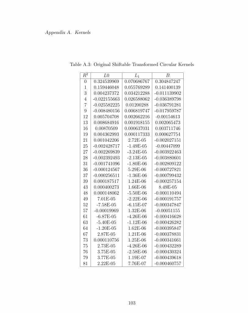
Appendix A. Kernels
Table A.3: Original Shiftable Transformed Circular Kernels
R2 L0 L1 B0 0.324539969 0.070686767 0.3048472471 0.159446048 0.055769289 0.1414001393 0.004237372 0.034212288 -0.0111399024 -0.022155663 0.026588062 -0.0363897987 -0.025582225 0.01200288 -0.0367912819 -0.008480156 0.006819747 -0.01795978712 0.005704708 0.002662216 -0.0015461313 0.008684916 0.001918155 0.00206547316 0.00870509 0.000637031 0.00371174619 0.004362993 0.000117333 0.00062775421 0.001042206 2.72E-05 -0.00202715125 -0.002428717 -1.49E-05 -0.0044709927 -0.002269839 -3.24E-05 -0.00392246328 -0.002392493 -2.13E-05 -0.00388060131 -0.001741096 -1.80E-06 -0.00280912236 -0.000124567 5.29E-06 -0.00072782137 -0.000256511 -1.36E-06 -0.00079943239 0.000187517 1.24E-06 -0.00025715443 0.000400273 1.66E-06 8.49E-0548 0.000148062 -5.50E-06 -0.00011049449 7.01E-05 -2.22E-06 -0.00019175752 -7.58E-05 -6.15E-07 -0.00034784757 -0.00019969 1.32E-06 -0.0005115561 -6.87E-05 -4.26E-06 -0.00041662863 -5.40E-05 -1.12E-06 -0.00042628264 -1.20E-05 1.62E-06 -0.00039584767 2.87E-05 1.21E-06 -0.00037883173 0.000110756 1.25E-06 -0.00034166175 2.73E-05 -4.26E-06 -0.00043228976 3.75E-05 -2.58E-06 -0.00043032479 3.77E-05 1.19E-07 -0.00043961881 2.22E-05 7.76E-07 -0.000460757
103

Appendix A. Kernels
Table A.4: Standard Shiftable Analytical Kernels
R2 L00 L03 L10 L13 BP BP11 BP13 BP3
0 52.349 75.487 100.487 145.594 350.347 0.000 0.000 0.0001 43.360 59.328 50.233 59.259 -7.702 110.880 87.958 26.5703 29.942 37.116 5.671 -6.364 -6.315 14.003 15.493 58.3864 24.777 29.021 -1.749 -12.955 -8.971 -8.848 -6.479 55.9047 13.263 11.532 -3.872 -4.886 -8.918 -4.126 -12.869 23.0159 8.019 3.917 -1.500 1.323 -4.659 7.889 -2.051 5.97412 2.762 -2.983 0.374 3.466 -0.408 7.158 4.577 -0.81213 1.554 -4.321 0.509 2.966 -0.107 3.781 3.794 0.19016 -0.872 -6.283 0.248 0.653 -1.366 -5.562 -2.100 5.36519 -2.008 -6.247 -0.128 -0.787 -3.013 -7.129 -6.325 7.45021 -2.299 -5.643 -0.218 -0.976 -3.204 -4.440 -6.448 6.19625 -2.212 -3.900 -0.104 -0.381 -1.460 2.060 -2.380 0.75627 -1.976 -2.971 -0.008 -0.019 -0.216 3.406 0.037 -1.64828 -1.832 -2.519 0.031 0.121 0.338 3.439 1.029 -2.51631 -1.358 -1.258 0.094 0.327 1.384 1.579 2.685 -3.57636 -0.624 0.380 0.047 0.153 0.924 -2.980 1.583 -1.64737 -0.504 0.626 0.028 0.091 0.626 -3.466 1.076 -1.06639 -0.301 1.030 -0.006 -0.021 -0.005 -3.760 0.074 -0.00843 -0.033 1.501 -0.043 -0.139 -0.919 -2.031 -1.205 1.13948 0.091 1.554 -0.029 -0.090 -0.836 1.481 -0.915 0.61349 0.098 1.512 -0.022 -0.067 -0.682 1.986 -0.679 0.35452 0.097 1.315 0.000 0.001 -0.107 2.717 0.129 -0.45957 0.072 0.871 0.020 0.062 0.684 1.450 1.100 -1.26961 0.054 0.515 0.017 0.053 0.780 -0.602 1.134 -1.13463 0.048 0.356 0.012 0.037 0.643 -1.500 0.929 -0.86464 0.045 0.283 0.009 0.028 0.539 -1.856 0.789 -0.69967 0.037 0.093 0.000 0.001 0.150 -2.436 0.302 -0.16973 0.008 -0.164 -0.009 -0.026 -0.539 -1.420 -0.465 0.56075 -0.006 -0.218 -0.009 -0.026 -0.635 -0.670 -0.551 0.61576 -0.014 -0.239 -0.008 -0.024 -0.651 -0.274 -0.558 0.60679 -0.040 -0.284 -0.005 -0.016 -0.577 0.849 -0.446 0.45381 -0.056 -0.299 -0.003 -0.009 -0.442 1.435 -0.287 0.275
104

Appendix A. Kernels
Table A.5: Standard Shiftable Transformed Kernels
R2 L00 L03 L10 L13
0 0.1213157 0.1796283 0.2383174 0.35345281 0.0999520 0.1362319 0.1261013 0.15249863 0.0740147 0.0949167 0.0235620 -0.00236684 0.0629760 0.0771331 0.0034145 -0.02377387 0.0373466 0.0368004 -0.0102020 -0.01896159 0.0252474 0.0186835 -0.0053700 -0.002168912 0.0124729 0.0010434 -0.0010006 0.006357113 0.0093152 -0.0028904 0.0002571 0.007530716 0.0022260 -0.0106809 0.0007705 0.004193719 -0.0021600 -0.0140476 0.0002413 0.000707821 -0.0038499 -0.0144258 -0.0003674 -0.001582225 -0.0052881 -0.0126307 -0.0004778 -0.001823227 -0.0052736 -0.0109188 -0.0002258 -0.001051128 -0.0051588 -0.0100081 -0.0001674 -0.000753631 -0.0044896 -0.0071132 0.0001474 0.000383636 -0.0029213 -0.0027010 0.0002768 0.000840637 -0.0026741 -0.0021331 0.0001175 0.000406939 -0.0020883 -0.0007630 0.0001213 0.000392143 -0.0011354 0.0012899 -0.0000589 -0.000163048 -0.0004711 0.0027398 -0.0000612 -0.000171549 -0.0003409 0.0029203 -0.0001064 -0.000313152 -0.0001060 0.0032678 -0.0000828 -0.000253157 0.0001028 0.0032639 0.0000195 0.000051761 0.0001913 0.0028823 0.0000294 0.000084063 0.0002108 0.0026041 0.0000481 0.000134264 0.0002066 0.0025059 0.0001129 0.000322367 0.0002199 0.0019643 0.0000622 0.000177073 0.0001870 0.0009406 -0.0000013 -0.000001475 0.0001371 0.0005725 -0.0000183 -0.000041576 0.0001239 0.0004373 -0.0000166 -0.000043179 0.0000794 0.0000741 -0.0000279 -0.000081781 0.0000604 -0.0001695 -0.0000755 -0.0002109
105

Appendix B
Matlab/Octave Filter Code
The Matlab program and Octave, its open source alternative, are well-suited to com-
puting with matrices and vectors. Additionally, Octave provides signal processing
tools such as the Fast Fourier Transform (FFT). The scripting language is almost
identical between Matlab and Octave, so that a script written for one should run
with few changes under the other. Work for this thesis used Octave almost exclu-
sively, since the available student version of Matlab contains no signal processing
tools without the separately purchased signal processing toolbox.
Construction of filters needs to be done relatively rarely, so that processing speed
is not a major consideration for most tasks. Moreover, filter construction requires
matrix manipulation and the FFT, depending on the method used. Since Octave
handles matrix and vector tasks easily, all of the filter construction tasks are im-
plemented in its scripting language. This section presents the tools necessary to
construct filters by the methods described in this thesis.
In this work, a filter is constructed from a one-dimensional transfer function. For
the original shiftable pyramid, where transfer function specifications are available,
explicit transfer functions are generated with Octave from the specifications. Where
106

Appendix B. Matlab/Octave Filter Code
only rectangular filter kernels are available, as for the standard shiftable pyramid,
Octave is used to generate the two-dimensional Fourier transform, which is the two-
dimensional transfer function that it is desired to resample. For each filter used in
the standard shiftable pyramid, the one-dimensional transfer function is obtained as
the cross section of the two-dimensional transfer function through its center.
Once a one-dimensional transfer function is obtained, either the direct inverse
polar Fourier transform or the McClellan transformation followed by an inverse
hexagonal Fourier transform (HFFT) may be used to produce a two-dimensional
filter kernel sampled on the hexagonal grid. In the first case, where the inverse
polar Fourier transform method is used, the result is also one-dimensional but cir-
cularly symmetric. To produce a two-dimensional hexagonally sampled kernel, the
procedure is to compute the distance from the center of each kernel point and then
compute the inverse polar Fourier transform at this distance. Of course, the ac-
tual algorithm avoids repeating computations by computing the kernel values for
all required distances before they are placed into the kernel. In the second case,
the McClellan transformation converts the one-dimensional transfer function into
a circularly-symmetric two-dimensional transfer function sampled on the hexagonal
grid. The inverse HFFT converts the hexagonal transfer function into the corre-
sponding hexagonal filter kernel.
B.1 Octave Code for Inverse Polar FT
The routines presented in the following implement or analyze this process. The first
listing presents the inverse polar Fourier transform. This function takes a 512-point
transfer function as input and returns a n × n matrix containing the values of the
kernel at the distance from the kernel center computed as rs(i, j) in the routine.
These distances are based on the hexagonal grid, and the values in the matrix are to
107

Appendix B. Matlab/Octave Filter Code
be interpreted as corresponding to these distances. The pyramid routines are set up
to read the output of radialb in this format.
As discussed in Chapter 3, the computation of an oriented kernel requires mul-
tiplying the kth order kernel for the kth term of the Fourier series of the angular
function by cos(kθ) and the Fourier series coefficient. To obtain the kth order ker-
nel, set the third argument equal to k and save the resulting matrix out to a file the
the pyramid software knows how to read. All of the band-pass kernel matrices are
written out to a file named with the same prefix, such as “t”. The order k should be
appended to this file name so that the software reads it automatically.
function [y,rs] = radialb(ampl,n,ord)
rs = zeros(n,n);
taps = zeros(1,2*n*n);
y = rs;
for i=1:n
for j=1:n
x = mod(i-1,2)*0.5 + (j-1);
x2 = x*x;
y2 = 0.75*(i-1)*(i-1);
rs(i,j) = x2+y2
end
end
for i=1:n
for j=1:n
freq = sqrt(rs(i,j));
if (taps(rs(i,j)+1) == 0)
bes = besselj(ord,[0:511]/512 * freq * pi);
rx = ampl .* [0:511]/512;
108

Appendix B. Matlab/Octave Filter Code
y(i,j) = rx * bes’;
taps(rs(i,j)+1) = y(i,j);
else
y(i,j) = taps(rs(i,j)+1);
end
end
end
end;
B.2 Kernel Size Estimation
The next listing presents a function that computes a matrix giving the extent to
which the output of the radialb function depends on each entry of the input kernel.
This information can be used to roughly predict the size of the output kernel given
the size of the input kernel.
function y = radspread(order,N)
y = zeros(N);
for nu=1:N
bes = besselj(order,[0:511]/512 * (nu-1) * pi);
for n=1:N
ampl = cos([0:511]/512 * (n-1) * pi);
if n > 1
ampl *= 2;
end
rx = ampl .* [0:511]/512;
y(nu,n) = rx * bes’;
end
109

Appendix B. Matlab/Octave Filter Code
end
y /= 64;
B.3 McClellan Transformation Scripts
The following two routines fqt and ftrans together implement the McClellan trans-
formation. The ftrans routine computes the location of each point on a hexago-
nal grid, and then it calls fqt with the location coordinates and the input one-
dimensional transfer function. The fqt function returns the transformed value of
the transfer function for the requested point, and ftrans places the value into the
output array representing the new hexagonal transfer function. The computation of
the point location by ftrans results in the construction of a hexagonal fundamental
period as described in Chapter 3.
function hy = fqt(w,x,y);
N = length(w);
sqt = sqrt(3);
x = x/2;
y = y/2;
hy = w(N);
h = -1/3+4/9*(cos(2*y/sqt)+cos(y/sqt+x)+cos(y/sqt-x));
r = acos(h)/pi*N*4/3+1;
ir = floor(r);
if ir < N
dr = r-ir;
dw = w(ir+1)-w(ir);
hy = w(ir)+dw*dr;
end
110

Appendix B. Matlab/Octave Filter Code
function hy = ftrans(w,N)
hy = zeros(N,3*N);
sqt = sqrt(3);
n = length(w);
hx = ones(N,3*N)*w(n);
for j=1:N
for i=1:N
x = (i-N)*pi/N*2;
y = (2*(j-N)/sqt-(i-N)/sqt)*pi/N*2;
if x*x + y*y <= 5.5*pi*pi
hx(i,j) = fqt(w,x,y);
end
end
end
for j=N+1:2*N
for i=1:N
x = (i-N)*pi/N*2;
y = (2*(j-N)/sqt-(i-N)/sqt)*pi/N*2;
if x*x + y*y <= 5.5*pi*pi
hx(i,j) = fqt(w,x,y);
end
end
end
for j=N+1:2*N
for i=1:N
x = (i-1)*pi/N*2;
y = (2*(j-2*N)/sqt-i/sqt+0.5/sqt)*pi/N*2;
111

Appendix B. Matlab/Octave Filter Code
if y >= i/sqt-2*N/sqt-1/sqt && x*x + y*y <= 5.5*pi*pi
hx(i,j) = fqt(w,x,y);
end
end
end
for j=2*N+1:3*N
for i=1:N
x = i*pi/N*2;
y = (2*(j-2*N+0.5)/sqt-i/sqt)*pi/N*2;
f x*x + y*y <= 5.5*pi*pi
hx(i,j) = fqt(w,x,y);
end
end
end
hy = ampl(shift(hx’,N)’);
B.4 HFFT Implementation
The following routines hdft, rhfft, and hfft implement the Hexagonal Fast Fourier
Transform (HFFT) as described by Mersereau [14]. The hdft function computes the
Hexagonal Discrete Fourier Transform (HDFT) as a sum, but it is extremely slow.
The rhfft function implements the recursive HFFT, constructing each stage of the
HFFT from HFFTs of one-quarter the size. It calls the hdft function when the size
of the input is a 2× 6 matrix. The top-level hfft sets up the top-level one-quarter
matrices and calls rhfft to begin the recursion.
function y = hdft(x,N,d)
[n,m] = size(x);
112

Appendix B. Matlab/Octave Filter Code
y = zeros(N,3*N);
for k1 = 0:3*N-1
for k2 = 0:N-1
for ni=0:n-1
for nj=0:m-1
w = d*pi*((2*nj-ni)*(2*k1-k2)/3/N + ni*k2/N);
y(k2+1,k1+1) = y(k2+1,k1+1) + x(ni+1,nj+1)*exp(-i*w);
end
end
end
end
function y = rhfft(x,N,d,wg,wh,wi)
[n,m] = size(x);
y = zeros(N,3*N);
N2 = N/2;
sf = zeros(N2, 3*N2);
sg = zeros(N2, 3*N2);
sh = zeros(N2, 3*N2);
si = zeros(N2, 3*N2);
wg2 = wg(1:2:N,1:2:3*N);
wh2 = wh(1:2:N,1:2:3*N);
wi2 = wi(1:2:N,1:2:3*N);
wgh = wg(1:N/2,1:3*N/2);
whh = wh(1:N/2,1:3*N/2);
wih = wi(1:N/2,1:3*N/2);
if N < 4
sf = hdft(x(1:2:n,1:2:m),N/2,d);
113

Appendix B. Matlab/Octave Filter Code
sg = wgh .* hdft(x(2:2:n,1:2:m),N/2,d);
sh = whh .* hdft(x(1:2:n,2:2:m),N/2,d);
si = wih .* hdft(x(2:2:n,2:2:m),N/2,d);
else
sf = rhfft(x(1:2:n,1:2:m),N/2,d,wg2,wh2,wi2);
sg = wgh .* rhfft(x(2:2:n,1:2:m),N/2,d,wg2,wh2,wi2);
sh = whh .* rhfft(x(1:2:n,2:2:m),N/2,d,wg2,wh2,wi2);
si = wih .* rhfft(x(2:2:n,2:2:m),N/2,d,wg2,wh2,wi2);
end
y(1:N/2,1:3*N/2) = sf + sg + sh + si;
y(1:N/2,1+3*N/2:3*N) = sf - sg + sh - si;
y(N/2+1:N,N+1:5*N/2) = sf + sg - sh - si;
s5 = sf - sg - sh + si;
y(N/2+1:N,5*N/2+1:3*N) = s5(1:N/2,1:N/2);
y(N/2+1:N,1:N) = s5(1:N/2,N/2+1:3*N/2);
function y = hfft(x,N,d)
wg = exp(i*2*d*pi/3/N*[0:3*N-1]);
wg = exp(-i*4*d*pi/3/N*[0:N-1]’)*wg;
wh = exp(-i*4*d*pi/3/N*[0:3*N-1]);
wh = exp(i*2*d*pi/3/N*[0:N-1]’)*wh;
wi = exp(-i*2*d*pi/3/N*[0:3*N-1]);
wi = exp(-i*2*d*pi/3/N*[0:N-1]’)*wi;
y = rhfft(x,N,d,wg,wh,wi);
114

Appendix B. Matlab/Octave Filter Code
B.5 Formatting a Hexagonal Fundamental Period
In order to process a kernel with the HFFT, it is necessary to reformat it from its
representation as a square matrix and embed it into a N × 3N matrix, where N
is the size of the desired transform. The rehex does this using the ihfftshift
to position the kernel correctly. For inverse transforms, the transfer function is
generated so that it already forms a correct hexagonal fundamental period. However,
the kernel resulting from the inverse HFFT must be extracted and reformatted from
its hexagonal fundamental period in order to be used by the pyramid software. The
unhex and hfftshift routines support these operations. At a higher level, the
l*gen.m and bp*gen.m routines illustrate the usage of the preceding functions in
generating low-pass and band-pass kernels. The rather trivial ampl function returns
the amplitude of a complex number.
function y = hfftshift(A)
[n,m] = size(A);
al = shift(A(1:n/2,:)’,2*n)’;
B = [al; A(n/2+1:n,:)];
y = shift(B,n/2);
function y = ihfftshift(A)
[n,m] = size(A);
y1 = shift(A’,n/2)’;
B = shift(y1,-n/2);
al = B(1:n/2,:);
z = B(n/2+1:n,:);
z1 = shift(al’,-2*n)’;
y = [z1; z];
115

Appendix B. Matlab/Octave Filter Code
function hx = rehex(A,N)
[n,m] = size(A);
hy = zeros(N,3*N);
c = floor(n/2);
hy(N/2-c+1:N/2+c+1,3*N/2-c+1:3*N/2+c+1) = A;
for i=1:n/2
hy(N/2+i+1,:) = shift(hy(N/2+i+1,:),floor((i+1)/2));
hy(N/2-i+1,:) = shift(hy(N/2-i+1,:),-floor(i/2));
end
hx = ihfftshift(hy);
function hy = unhex(A)
[n,m] = size(A);
cA = hfftshift(A);
ccA = cA(:,2*n-n/2+1:2*n+n/2);
hy = zeros(n);
for i=1:n
for j=1:n
y = j + floor(i/2);
if (y < n)
hy(i,j) =ccA(i,y);
end
end
end
function y = ampl(A)
y = sqrt(A .* conj(A));
116

Appendix B. Matlab/Octave Filter Code
function y = l1gen(kernel,N,m)
h1 = fft2(kernel,1024,1024);
hx1 = ftrans(ampl(h1(1,1:512)),N);
b1 = hfft(hx1,N,-1)/N/N/3;
ub1 = unhex(real(b1));
midx = N/2+1;
midy = N/4+1;
y = ub1(midx-m:midx+m,midy-m:midy+m);
function y = bpgen(kernel,N,m)
hb = fft2(kernel,2048,2048);
cb = 1-ampl(hb);
cxb = ftrans(cb(1,1:1024),N);
bb = hfft(1-cxb,N,-1)/N/N/3;
ubb = unhex(real(bb));
midx = N/2+1;
midy = N/4+1;
y = ubb(midx-m:midx+m,midy-m:midy+m);
B.6 Oriented Filter Kernels
To generate oriented kernels, it is necessary to follow the procedure for the inverse
polar Fourier transform method, which multiplies the terms corresponding to the
Fourier series of the angular function by the appropriate Fourier basis function, or
to multiply the two-dimensional hexagonal transfer function by the angular function
in the frequency domain and then perform the inverse HFFT. The routines listed in
117

Appendix B. Matlab/Octave Filter Code
the following support the latter procedure, since the inverse polar Fourier transform
is supported by radialb as described in the preceding.
The coshex0 and sinhex0 routines multiply the radial component of the two-
dimensional transfer function by cos(θ) or sin(θ), respectively to produce the first
order derivative oriented transfer functions. Only the coshex0 function is shown
here, since the sinhex0 function differs from it only in the multiplying function
and both are rather lengthy. The coshex3 similarly generates the requested basis
transfer functions for the third order derivative oriented filter. The cos3 function
supports coshex3 with a fast cos3(θ) calculation. The high level bp*gen functions
automate construction of the oriented filters and serve to illustrate the usage of the
preceding. To use the bp*gen load in the appropriate rectangular band-pass kernel.
The standard shiftable pyramid uses a different set of filters for each angular function,
so that not only the band-pass kernels but the low-pass kernels must be switched out
when changing the order of the steerable filter. Only orders 0, 1, and 3 are supported
by the standard shiftable pyramid.
function SR = coshex0(B)
[N,M] = size(B);
A = shift(B’,-N)’;
rcenter = 1;
ccenter = 1;
R = zeros(N,M);
sqt = sqrt(3.0);
for j=1:N
for i=1:N
x = sqt*(i-N)/2;
y = j-i/2-N/2;
r = sqrt(x*x+y*y);
118

Appendix B. Matlab/Octave Filter Code
if r != 0.0
R(i,j) = A(i,j)*y/r;
end
end
end
for j=N+1:2*N
for i=1:N
x = sqt*(i-N)/2;
y = j-i/2-N/2;
r = sqrt(x*x+y*y);
if r != 0.0
R(i,j) = A(i,j)*y/r;
end
end
end
for j=N+1:2*N
for i=1:N
x = sqt*i/2;
y = j-i/2-2*N+0.5;
r = sqrt(x*x+y*y);
if y >= i/2-N-0.5 && r != 0
R(i,j) = A(i,j)*y/r;
end
end
end
for j=2*N+1:3*N
for i=1:N
x = sqt*i/2;
119

Appendix B. Matlab/Octave Filter Code
y = j-i/2+0.5-2*N;
r = sqrt(x*x+y*y);
if r != 0.0
R(i,j) = A(i,j)*y/r;
end
end
end
SR = shift(R’,N)’;
function z = cos3(x,y,r,cosoff,sinoff)
cos1 = x/r;
sin1 = y/r;
coff = cos1*cosoff+sin1*sinoff;
z = coff*coff*coff;
function SR = coshex3(B,k)
[N,M] = size(B);
off = k*pi/4;
cosoff = cos(off);
sinoff = sin(off);
A = shift(B’,-N)’;
rcenter = 1;
ccenter = 1;
R = zeros(N,M);
sqt = sqrt(3.0);
for j=1:N
for i=1:N
x = sqt*(i-N)/2;
120

Appendix B. Matlab/Octave Filter Code
y = j-i/2-N/2;
r = sqrt(x*x+y*y);
if r != 0.0
R(i,j) = A(i,j)*cos3(y,x,r,cosoff,sinoff);
end
end
end
for j=N+1:2*N
for i=1:N
x = sqt*(i-N)/2;
y = j-i/2-N/2;
r = sqrt(x*x+y*y);
if r != 0.0
R(i,j) = A(i,j)*cos3(y,x,r,cosoff,sinoff);
end
end
end
for j=N+1:2*N
for i=1:N
x = sqt*i/2;
y = j-i/2-2*N+0.5;
r = sqrt(x*x+y*y);
if y >= i/2-N-0.5 && r != 0
R(i,j) = A(i,j)*cos3(y,x,r,cosoff,sinoff);
end
end
end
for j=2*N+1:3*N
121

Appendix B. Matlab/Octave Filter Code
for i=1:N
x = sqt*i/2;
y = j-i/2+0.5-2*N;
r = sqrt(x*x+y*y);
if r != 0.0
R(i,j) = A(i,j)*cos3(y,x,r,cosoff,sinoff);
end
end
end
SR = shift(R’,N)’;
function y = bp0gen(kernel,N,m)
hb = fft2(kernel,2048,2048);
hxb = ftrans(ampl(hb(1,1:1024)),N);
chxb = coshex0(hxb);
cbb = hfft(chxb,N,-1)/N/N/3;
cubb = unhex(imag(cbb));
midx = N/2+1;
midy = N/4+1;
y = cubb(midx-m:midx+m,midy-m:midy+m);
function y = bp3gen(kernel,N,m,k)
hb = fft2(kernel,2048,2048);
hxb = ftrans(ampl(hb(1,1:1024)),N);
chxb = coshex3(hxb,k);
cbb = hfft(chxb,N,-1)/N/N/3;
cubb = unhex(imag(cbb));
midx = N/2+1;
122

Appendix B. Matlab/Octave Filter Code
midy = N/4+1;
y = cubb(midx-m:midx+m,midy-m:midy+m);
B.7 Kernel Refinement
The radialize function produces a kernel that is circularly symmetric from one
that is nearly so. Kernel values at a given distance from center are averaged and the
result written to all the entries at that distance. The hexagonalize routine returns
a kernel for which all kernel positions outside the specified distance from the center
are set to zero.
function y = radialize(A)
[n,n] = size(A);
mid = (n+1)/2;
rs = zeros(n);
taps = zeros(1,2*n*n);
count = zeros(1,2*n*n);
y = rs;
for i=1:n
for j=1:n
x = mod(abs(i-mid),2)*0.5 + j-mid;
x2 = x*x;
y2 = 0.75*(i-mid)*(i-mid);
rs(i,j) = x2+y2;
end
end
for i=1:n
for j=1:n
123

Appendix B. Matlab/Octave Filter Code
if (rs(i,j) != 0)
taps(rs(i,j)) = (taps(rs(i,j))*count(rs(i,j)) +
A(i,j))/(count(rs(i,j))+1);
count(rs(i,j)) += 1;
end
end
end;
for i=1:n
for j=1:n
if (rs(i,j) == 0)
y(i,j) = A(mid,mid);
else
y(i,j) = taps(rs(i,j));
end
end
end;
function y = hexagonalize(A)
[n,n] = size(A);
layers = (n-1)/2;
mid = layers+1;
y=A;
for i=1:layers
for j=1:floor(i/2)
y(mid+i,j)=0.0;
y(mid-i,j)=0.0;
end
for j=n-floor((i-1)/2):n
124

Appendix B. Matlab/Octave Filter Code
y(mid+i,j)=0.0;
y(mid-i,j)=0.0;
end
end
B.8 Accuracy Measurement
The qual routine reads the original and reconstructed images written out to files
by the pyramid program. It computes the maximum difference, the mean square
difference, and the difference image from the two images. The qual computes these
figures for the center one quarter of the image, assuming a square image and given
one dimension as input. The oqual routine computes the same results for the entire
image. For the test images, which have a black border of one quarter the image
dimension, the qual routine provides measurement of the best possible reconstruc-
tion accuracy that eliminates almost all edge effects. The oqual routine provides a
measurement of how edge effects grow with pyramid depth.
function [y,var,logvar,d] = qual(N)
load p1.mat p1;
load p0.mat p0;
d = p1-p0;
em = N/2-N/4;
ep = N/2+N/4;
ds = d(em:ep,em:ep);
y = max(max(abs(ds)));
var = sum(sum(ds .* ds))/N/N*4;
logvar = 10*log10(var);
125

Appendix B. Matlab/Octave Filter Code
function [y,var,logvar,d] = oqual(N)
load p1.mat p1;
load p0.mat p0;
d = p1-p0;
y = max(max(abs(d)));
var = sum(sum(d .* d))/N/N;
logvar = 10*log10(var);
B.9 Miscellaneous Matlab/Octave Routines
The resample function resamples an input function by linear interpolation so that its
values at the specified number of points, spaced uniformly, are returned as a vector.
This routine is used mainly to display a transfer function computed by HFFT of
hexagonal kernels with the original desired transfer function.
function y = resample(h,N)
n = length(h);
for i=0:N-1
y(i+1) = linterp(h,(i/N)*(n-1)+1);
end
126

References
[1] E.H. Adelson, C.H. Anderson, J.R. Bergen, P.J. Burt, and J.M. Ogden, PyramidMethods in Image Processing, RCA Engineer 29 (1984), no. 6, 33–41.
[2] Anonymous author, Parks-McClellan Filter Design, 2005, Available online athttp://www.dsptutor.freeuk.com/remez/RemezFIRFilterDesign.html.
[3] Ronald N. Bracewell, The Fourier Transform and Its Applications, McGraw-HillBook Company, 1978.
[4] K. R. Castleman, M. Schulze, and Q. Wu, Simplified Design of Steerable PyramidFilters, Proceedings - IEEE International Symposium on Circuits and Systems,vol. 67, 1979, pp. 930–949.
[5] Kenneth R. Castleman, Digital image processing, Prentice Hall, Inc., 1996.
[6] Zoran Cvetkovic and Martin Vetterli, Oversampled Filter Banks, IEEE Trans-actions on Signal Processing 46 (1998), no. 5, 1245–1255.
[7] William T. Freeman and Edward H. Adelson, The Design and Use of Steer-able Filters, IEEE Transactions on Pattern Analysis and Machine Intelligence9 (1991), 891–906.
[8] Branko Grunbaum and G. C. Shephard, Tilings and Patterns, W. H. Freemanand Company, 1987.
[9] Innchyn Her, Chin-Chung Huang, and Rong-Da Hsieh, A Simulated Fast Hexag-onal Fourier Transform, IEICE Transactions on Fundamentals of Electronics,Communications and Computer Sciences E870A (2004), no. 7, 1804–1809.
[10] Anestis Karasaridis and Eero Simoncelli, A Filter Design Technique for SteerablePyramid Image Transforms, Proceedings of the ICASSP-96, 1996, pp. 2387–2390.
127

References
[11] H. Knutsson and G.H. Granlund, Texture Analysis using Two-dimensionalQuadrature Filters, IEEE Computer Society Workshop on Computer Architec-tures for Pattern Analysis and Image Database Management, 1983, pp. 206–213.
[12] Jae S. Lim, Two-Dimensional Signal and Image Processing, Prentice Hall, 1990.
[13] Wu-Sheng Lu and Andreas Antoniou, Two-Dimensional Digital Filters, MarcelDekker, Inc., 1992.
[14] Russell M. Mersereau, The Processing of Hexagonally Sampled Two-Dimensional Signals, Proceedings of the IEEE, vol. 5, 1978, pp. 329–332.
[15] Lee Middleton and Jayanthi Sivaswamy, Framework for Practical Hexagonal-Image Processing, Journal of Electronic Imaging 11 (2002), no. 1, 104–114.
[16] T. W. Parks and C. S. Burrus, Digital Filter Design, John Wiley and Sons, Inc.,1987.
[17] William H. Press, Brian P. Flannery, Saul A. Teukolsky, and William T. Vet-terling, Numerical Recipes (FORTRAN Version), Cambridge University Press,1989.
[18] Markus Puschel and Martin Rotteler, Cooley-Tukey FFT like Algorithm for theDiscrete Triangle Transform, 2004 IEEE 11th Digital Signal Processing Work-shop, 2004, pp. 158–162.
[19] G.E. Rivard, Direct Fast Fourier Transform of Bivariate Functions, IEEE Trans-actions on Acoustics, Speech, and Signal Processing ASSP-25 (1977), no. 3,250–252.
[20] Eero P. Simoncelli, C source code, 2006, Available online athttp://www.cns.nyu.edu/pub/eero/steerpyr.tar.gz.
[21] Eero P. Simoncelli and Hany Farid, Steerable Wedge Filters for Local OrientationAnalysis, IEEE Transactions on Image Processing 5 (1996), no. 9, 1377–1382.
[22] Eero P. Simoncelli, William T. Freeman, Edward H. Adelson, and David J.Heeger, Shiftable Multiscale Transforms, IEEE Transactions on InformationTheory 38 (1992), no. 2, 587–607.
[23] Elias M. Stein and Guido Weiss, Introduction to Fourier Analysis on EuclideanSpaces, Princeton University Press, 1971.
[24] John Woods (ed.), Subband Coding, Kluwer Academic Press, 1990.
128