implementation of a solar collectorarchbps1.campus.tue.nl/bpswiki/images/7/7c/7y700_2012_3_r.pdf ·...

Implementation of a solar collector

Semi-detached dwelling

Eindhoven University of Technology

Course code: 7Y700

Course name: Sustainable building and systems modelling

Student / Author 1: Ing. J.J. Groeneveld Student number: 0756388

E-mail: [email protected]

Student / Author 2: Ing. F.T. van Schie Student number: 0751230

E-mail: [email protected]

Issue: Eindhoven, 17 July 2012 Version: V1.0

F.T. van Schie 17-7-2012

- II -

CONTENT

1 Introduction ............................................................................................................................ 3

2 Current situation .................................................................................................................... 4

2.1 Building services ........................................................................................................... 4

2.2 Parameters ................................................................................................................... 5

2.3 Results .......................................................................................................................... 5

3 New situation .......................................................................................................................... 6

3.1 Building services ........................................................................................................... 6

3.2 Parameters ................................................................................................................... 7

3.2.1 Flat plate collector ............................................................................................. 7

3.2.2 Vacuum tube collector ...................................................................................... 7

3.2.3 Plastic collector ................................................................................................. 7

3.2.4 Efficiency collectors .......................................................................................... 7

3.3 Results .......................................................................................................................... 8

3.3.1 Weekly simulation ............................................................................................. 8

3.3.2 Yearly simulation .............................................................................................. 9

4 Conclusion / discussion ...................................................................................................... 11

5 References ............................................................................................................................ 12

Appendix I – Floor plans Appendix II – Script with parameters

J.J. Groeneveld and F.T. van Schie 17-7-2012

- 3 -

1 INTRODUCTION

The objectives of this report are to investigate and simulate the current annual energy demand

of a building and improve the energy performance by applying sustainable measures without compromising on a comfortable indoor climate.

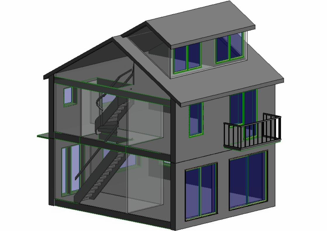
The chosen building is the parental home of Johan, which is shown in figure 1. The building is located in Soest. The floor plans with the marked rooms of the building are included in appendix I.

The sustainable measurement which is taken into account is a solar boiler. There are three types of solar boilers used in the simulations, namely:

• Flat plate collector;

• Vacuum collector;

• Plastic collector.

Figure 1: Parental home of Johan

The current energy demand of Johan’s parental home is simulated and compared with actual results of the energy consumption. A solar boiler is implemented in the existing climate system. New simulations are made and compared with the previous results. An advice and conclusion will be given in the end of the report.


- 4 -

2 CURRENT SITUATION

Johan’s parental dwelling used for the simulation consists of three floors divided in five zones, namely: 1. Living room; 2. Hallway; 3. Bedroom; 4. Bathroom; 5. Hobby room.

2.1 Building services The heating installation in the dwelling is a boiler in combination with radiators. Each room has

its own radiator. Appendix IV provides a pipes and instruments diagram of the existing situation. In figure 3 is a schematic overview given of the existing system.

Figure 2: Pipes and instruments diagram of the current system

Figure 3 shows a schematic overview of the current system.

Figure 3: Schematic overview of the current system

Based on figure 3 the ODE’s are determined. The corresponding ODE’s are as follows:

��

�� ∙ � ∙ �6�� ∙ � ∙ �4� ��

��

�� ∙ � ∙ �5�� ∙ � ∙ �6� ��


- 5 -

2.2 Parameters

The internal temperature for each room is set at 19°C. In the current situation the thermostat is positioned in the living room. When the desired temperature in the living room is reached, the boiler is switched off. The other rooms could still need heat, but no heat can be delivered. Lower temperatures than the desired temperature of 19°C in the other rooms of the dwelling can be reached.

The boiler provides a constant temperature of 85°C. The boiler is combined with a separate wood stove, located in the living room. The wood stove uses wood instead of gas to heat the building.

The dimensions and floor plans of the dwelling are given in appendix I. The script with the parameters used for the simulation is shown in appendix II

2.3 Results Figure 4 shows the results of the simulated and measured gas consumption. The simulated

values differ from the calculated values. The difference can be explained by multiple causes, like:

• The usage of domestic hot water is not included by the simulations results;

• The results of the simulation are based on another climate year;

• The heat production of the wood stove is not taken into account with the results of the simulation.

The wood stove which is positioned in the living room is mostly used in the winter. The wood stove heats only the living room, where also the thermostat is positioned. If the thermostat reaches the desired temperature, due the heating of the wood stove, the temperature will not be heated by the boiler. With these summed differences, the simulated and measured gas consumption still have the same trends.

Figure 4: Simulated and measured gas consumption

0

20

40

60

80

100

120

140

1 7 13 19 25 31 37 43 49

V [

m3]

t [week]

Simulated and measured gas consumption

Matlab (1984)

2010

2011


- 6 -

3 NEW SITUATION

A solar collector system is added to the dwelling to safe gas for heating. First, a research is done about which type of solar collector is most efficient for the conditions in the Netherlands. Second, the usage of a low temperature radiator system has been investigated.

3.1 Building services Figure 5 shows a pipes and instruments diagram of the integration of a solar collector and a

buffer within the current system.

Figure 5: Pipes and instruments diagram of the new system

Figure 6 shows the extended model of the new system. As shown in figure 6 the solar collector with a buffer is integrated in the schematic overview.

Figure 6: Schematic overview of the new system


- 7 -

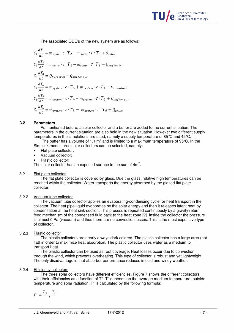
The associated ODE’s of the new system are as follows:

��

�� ∙ � ∙ �2�� ∙ � ∙ �1 � ��

�"��"

�� ∙ � ∙ �1 �� ∙ � ∙ �2� ��#$$��%

�&��&

�� #$$��% � ��#$$��#�

��

�� ∙ � ∙ �6�� ∙ � ∙ �4� ��

�'��'

�� ∙ � ∙ �4 �� ∙ � ∙ �5� ��#$$��#�

��

�� ∙ � ∙ �5�� ∙ � ∙ �6� ��

3.2 Parameters

As mentioned before, a solar collector and a buffer are added to the current situation. The parameters in the current situation are also held in the new situation. However two different supply temperatures in the simulations are used, namely a supply temperature of 85°C and 45°C.

The buffer has a volume of 1.1 m3 and is limited to a maximum temperature of 95°C. In the

Simulink model three solar collectors can be selected, namely:

• Flat plate collector;

• Vacuum collector;

• Plastic collector; The solar collector has an exposed surface to the sun of 4m

2.

3.2.1 Flat plate collector

The flat plate collector is covered by glass. Due the glass, relative high temperatures can be reached within the collector. Water transports the energy absorbed by the glazed flat plate collector.

3.2.2 Vacuum tube collector The vacuum tube collector applies an evaporating-condensing cycle for heat transport in the

collector. The heat pipe liquid evaporates by the solar energy and then it releases latent heat by condensation at the heat sink section. This process is repeated continuously by a gravity return feed mechanism of the condensed fluid back to the heat zone [2]. Inside the collector the pressure is almost 0 Pa (vacuum) and thus there are no convection losses. This is the most expensive type of collector.

3.2.3 Plastic collector The plastic collectors are nearly always dark colored. The plastic collector has a large area (not

flat) in order to maximize heat absorption. The plastic collector uses water as a medium to transport heat.

The plastic collector can be used as roof coverage. Heat losses occur due to convection through the wind, which prevents overheating. This type of collector is robust and yet lightweight. The only disadvantage is that absorber performance reduces in cold and windy weather.

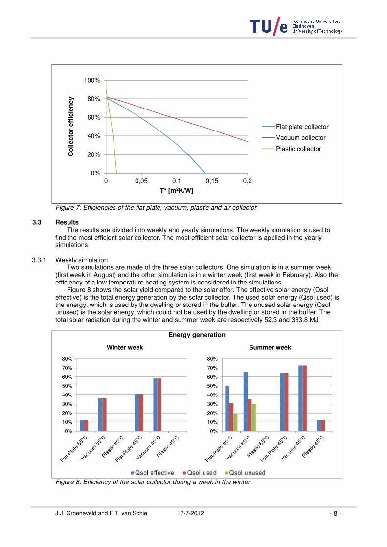
3.2.4 Efficiency collectors The three solar collectors have different efficiencies. Figure 7 shows the different collectors

with their efficiencies as a function of T*. T* depends on the average medium temperature, outside temperature and solar radiation. T* is calculated by the following formula:

�∗ ��

)


- 8 -

Figure 7: Efficiencies of the flat plate, vacuum, plastic and air collector

3.3 Results The results are divided into weekly and yearly simulations. The weekly simulation is used to

find the most efficient solar collector. The most efficient solar collector is applied in the yearly simulations.

3.3.1 Weekly simulation Two simulations are made of the three solar collectors. One simulation is in a summer week

(first week in August) and the other simulation is in a winter week (first week in February). Also the efficiency of a low temperature heating system is considered in the simulations.

Figure 8 shows the solar yield compared to the solar offer. The effective solar energy (Qsol effective) is the total energy generation by the solar collector. The used solar energy (Qsol used) is the energy, which is used by the dwelling or stored in the buffer. The unused solar energy (Qsol unused) is the solar energy, which could not be used by the dwelling or stored in the buffer. The total solar radiation during the winter and summer week are respectively 52.3 and 333.8 MJ.

Energy generation

Figure 8: Efficiency of the solar collector during a week in the winter

0%

20%

40%

60%

80%

100%

0 0,05 0,1 0,15 0,2

Co

llecto

r eff

icie

ncy

T* [m2K/W]

Flat plate collector

Vacuum collector

Plastic collector

0%

10%

20%

30%

40%

50%

60%

70%

80%

Winter week

0%

10%

20%

30%

40%

50%

60%

70%

80%

Summer week


- 9 -

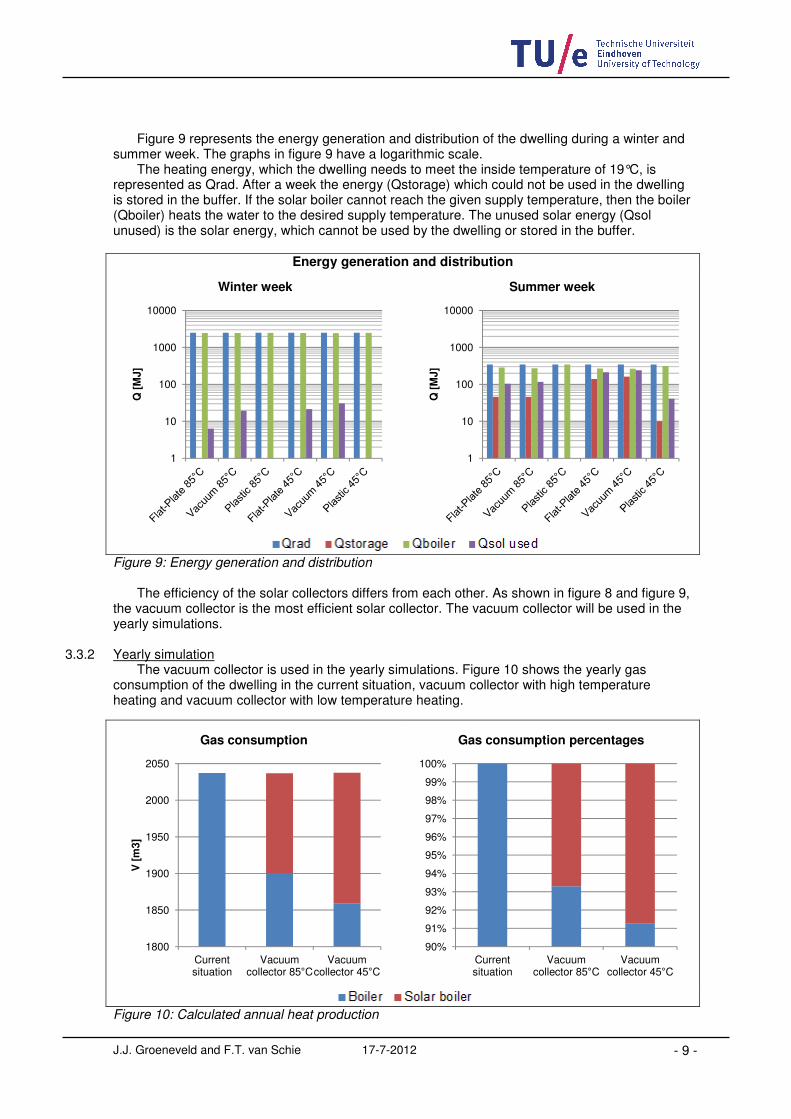
Figure 9 represents the energy generation and distribution of the dwelling during a winter and summer week. The graphs in figure 9 have a logarithmic scale.

The heating energy, which the dwelling needs to meet the inside temperature of 19°C, is represented as Qrad. After a week the energy (Qstorage) which could not be used in the dwelling is stored in the buffer. If the solar boiler cannot reach the given supply temperature, then the boiler (Qboiler) heats the water to the desired supply temperature. The unused solar energy (Qsol unused) is the solar energy, which cannot be used by the dwelling or stored in the buffer.

Energy generation and distribution

Figure 9: Energy generation and distribution

The efficiency of the solar collectors differs from each other. As shown in figure 8 and figure 9, the vacuum collector is the most efficient solar collector. The vacuum collector will be used in the yearly simulations.

3.3.2 Yearly simulation The vacuum collector is used in the yearly simulations. Figure 10 shows the yearly gas

consumption of the dwelling in the current situation, vacuum collector with high temperature heating and vacuum collector with low temperature heating.

Figure 10: Calculated annual heat production

1

10

100

1000

10000

Q [

MJ]

Winter week

1

10

100

1000

10000

Q [

MJ]

Summer week

1800

1850

1900

1950

2000

2050

Current situation

Vacuum collector 85°C


V [

m3]

Gas consumption

90%

91%

92%

93%

94%

95%

96%

97%

98%

99%

100%

Current situation



Gas consumption percentages


- 10 -

As shown by the simulations of the vacuum collector, the gas consumption is lowered. Table 1 shows the savings on gas over a year. The gas price is considered at € 0.6468 for a dwelling [3]. The total savings on money are also shown in table 1. Table 1: Yearly savings on gas and money

Vacuum collector Savings on gas a year Yearly savings

High temperature heating 136 [m3] € 88,19

Low temperature heating 178 [m3] € 115,23

Figure 11 shows the annual solar heat generation. The left graph shows the total solar

radiation (Qsol total) against the vacuum collectors. The solar radiation of the vacuum collectors is divided into:

• Used solar radiation;

• Unused solar radiation;

• Not collectable radiation. The used solar radiation is used in the dwelling. The unused solar radiation is the energy, which could be collected by the solar boiler, but the energy could be stored in the buffer. The buffer has reached its limit of 95°C. The not collectable radiation is the radiation, which has radiated on the surface, but could not be collected due the efficiency of the solar collector.

Figure 11: Annual solar heat generation

The total annual efficiency of the vacuum collector is for a high and low heating system respectively 43% and 56%. When the volume of the buffer could increase, the total annual efficiency could increase respectively to 62% and 69%.

0

50

100

150

200

250

300

350

Qsol total Vacuum collector 85°C


V [

m3]

Solar radiation

0%

10%

20%

30%

40%

50%

60%

70%

80%

90%

100%

Qsol total Vacuum collector 85°C


Solar radiation percentage


- 11 -

4 CONCLUSION / DISCUSSION

The efficiency of the flat plate, vacuum and plastic collector differs from each other. In the weekly simulations the vacuum collector is the most efficient solar collector.

The vacuum collector combined with a high temperature heating system is less efficient than the low temperature heating system. The efficiency could be increased by using a buffer with a larger volume. However, using a larger volume gives a larger heat loss.

If a low temperature heating system is applied, the surface of the radiators in the rooms should be larger to supply the same amount of power. A low temperature heating system requires a higher initial investment.

Gas is a fossil fuel, which is running down; therefore the price of gas is rising. When the price of gas rises, the payback period of the vacuum collector would be less.

Hambase calculates with an upper heating value of 35.17 MJ/m

3 (9.8 kWh/m3) for gas.

Officially the simulations should take the under heating value of gas. The under heating value for gas is 31.65 MJ/m

3 (8.8 kWh/m3). The under heating value is lower than the upper heating value,

which causes a higher gas consumption. Different aspects are not taken into account In the Simulink model, like:

• The woodstove;

• The domestic water heating;

• The heat loss of the buffer;

• The extra electricity consumption of the solar boiler pump.


- 12 -

5 REFERENCES

[1] M.G.C.L. Loomans, Reader solar energy in the built environment, course 7S815, 2011. [2] www.thermotechs.com [3] www.nuon.nl


APPENDIX I – FLOOR PLANS 1. Total impression of the house 2. First floor

3. Second floor

4. Third floor


APPENDIX II – SCRIPT WITH PARAMETERS

2-7-12 13:48 D:\My Programs\Dropbox\7Y700 - Sustainable ...\CasestudyV09.m 1 of 12

% Case study for 7Y700 Building system modeling with standard wavo_output

% ------------------------------------------------------------------------

% HAMBASE

%

% HEAT And Moisture Building And Systems Evaluation

% -------------------------------------------------------------------------

% BUILDINGref

%

% Example input file to specify the building, profiles, systems are off

% The name of this m-file can be changed at wish.

% ------------------------------------------------------------------------------

% PART 1 : THE CALCULATION PERIOD

% -------------------------------------------------------------------------

% The available climate data of De Bilt are of the years 1971 till 2000. If the

% climate files of a different location are used the name and format must be

% adapted and the geographical coordinates must be changed (in InClimate-file).

% As an average year can be considered 1 May 1974 till 30 April 1975.

% A cold winter (242 days) started 1 September 1978.

% A hot summer (123 days) started 1 May 1976.

% 9 hot days started at 1 July 1976 and 9 cold days started at 30 December 1978.

%

% FORMAT BAS.Period=[yr,month,day,ndays]

%

% yr = start year

% month = start

% month day = start day

% ndays = number of days simulated

%BAS.Period=[1976,1,1,90,1];

BAS.Period=[1984,1,1,365];

% If BAS.DSTime=1 the EU daylight-savings time is taken into account. It starts on

the

% last Sunday of March and ends on the the last Sunday of October (the total

% duration is 30 or 31 weeks). If there is no daylight-savings period BAS.DSTime=0

% If the daylight-savings period is different from the EU the starting and ending

days

% must be given:

% BAS.DSTime(1,:)=[year,starting month,day,ending month,day];

% BAS.DSTime(2,:)=[year+1,starting month,day,ending month,day]; etc.

%BAS.DSTime(1,:)=[1987,4,28,4,29];

%BAS.DSTime(2,:)=[1988,4,3,4,3];

BAS.DSTime=1;

% ------------------------------------------------------------------------- ---

% PART 2 : THE BUILDING

% ------------------------------------------------------------------------- ---

% ZONES NUMBERS [-] & VOLUMES [m3]

%


% A zone consist of a room or several adjacent rooms with oubout the same

% temperature and relative humidity and the same climate control e.g. a dwelling

% might have three zones: the ground floor (living room etc), the first floor

% (sleeping) and the attic (not heated). There is however no restriction in the

% number of zones that can be simulated. Example: three zones: BAS.Vol{1}=..;

% BAS.Vol{2}=..; BAS.Vol{3}=.. If alone 2: use '%' for 1 and 3 so only

% BAS.Vol{2} remains.

%

% FORMAT BAS.Vol{zonenumber}=volume (m3);

BAS.Vol{1}= 87.09; % livingroom 32,7%

BAS.Vol{2}= 38.87; % hall 14,6%

BAS.Vol{3}= 70.47; % sleeping rooms 26,4%

BAS.Vol{4}= 7.52; % bathroom 2,8%

BAS.Vol{5}= 62.73; % top floor 23,5%

% total volume 266,68 m3

% ** CONSTRUCTION COMPONENTS DATA **

%

% A construction component usually consists of different layers. The order of

% the input of the properties of these layers is standard from indoors to

% outdoors and for construction components between zones from the zone with the

% lowest zone-number to the highest so: 1->2,1->3,2->3etc.. The material

% properties of the component layer are inserted by a material ID-number. By

% typing 'help matpropf' a list of materials appear with a material ID-number.

% Also each different construction component gets a different construction

% ID-number: conID=1,2,....

%

% FORMAT BAS.Con{conID}=[Ri,d1,matID,...,dn,matID,Re,ab,eb].

% dn = material layer thickness [m]

% matn = material ID-number.

% Ri = internal surface heat transfer resistance (for example Ri=0.13) [Km2/W]

% Re = surface heat transfer resistance at the opposite site (for example Re=0.04)

[Km2/W]

% ab = external solar radiation absorption coefficient [-] e.g.light ab=0.4, dark

ab=0.9.

% eb = external longwave emmisivity [-]. Almost always: eb=0.9

% BAS.Con{conID}=[Ri, d1, matID,... , dn, matID, Re,

ab, eb].

BAS.Con{1} = [0.13, 0.010,381, 0.100,238, 0.070,003, 0.100,238, 0.04,

0.9, 0.9];

BAS.Con{2} = [0.13, 0.010,381, 0.220,238, 0.010,381, 0.13,

0.5, 0.9];

BAS.Con{3} = [0.13, 0.030,501, 0.13,

0.5, 0.9];

BAS.Con{4} = [0.13, 0.080,342, 0.13,

0.5, 0.9];

BAS.Con{5} = [0.13, 0.013,381, 0.090,408, 0.018,501, 0.04,

0.9, 0.9];

BAS.Con{6} = [0.13, 0.019,381, 0.600,461, 0.040,003, 0.200,628, 0.04,

0.9, 0.9];

BAS.Con{7} = [0.13, 0.100,238, 0.13,

0.5, 0.9];

BAS.Con{8} = [0.13, 0.070,238, 0.13,

0.5, 0.9];


BAS.Con{9} = [0.13, 0.030,501, 0.200,001, 0.030,501, 0.13,

0.5, 0.9];

BAS.Con{10}= [0.13, 0.040,501, 0.04,

0.8, 0.9];

BAS.Con{11}= [0.13, 0.040,505, 0.13,

0.6, 0.9];

% dubbele wand (100 steen 80 spouw 100 steen)

% dubbel glas

% deur

% Commments

% 1: limestone,insulation,air gap,brick (external wall)

% 2: plaster,insulation,plaster (internal wall)

% 3: light concrete (internal wall, not used in this example)

% 4: tiles, limestone (internal wall, not used in this example)

% 5: limestone, insulation, air gap, hard brick (external wall)

% 6: roof construction

% 7: floor construction

% 8: floor construction

% 9: plaster, system floor, air gap, medium hardboard (floor between zones)

% 10: floor between zones

% 11: exterior door

% 12: interior door

% ** GLAZING SYSTEMS DATA**

%

% The solar gain factor of glazing depends on the incident angle of the solar

% radiation. The properties below are independent of this angle but if one wants

% to account for the incident angle this can be done with the shadow section

% (below). Each different glazing system gets an ID-number: glaID=1,2,.

%

% FORMAT BAS.Glas{glaID}=[Uglas,CFr,ZTA,ZTAw,CFrw,Uglasw]

%

% Uglas = U-value without sunblinds [W/m2K]

% CFr = convection factor without blinds [-]

% ZTA = Solar gain factor [-] without blinds

% ZTAw = Solar gain factor [-] with blinds

% CFrw = convection factor with blinds [-]

% Uglasw = U-value with blinds [W/m2K]

%

%BAS.Glas{glaID}= [Uglas, CFr, ZTA, ZTAw, CFrw, Uglasw]

BAS.Glas{1}= [3.0, 0.03, 0.6, 0.5, 0.15, 2.0 ];

BAS.Glas{2}= [4.5, 0.01, 0.80, 0.31, 0.34, 4.5 ];

BAS.Glas{3}= [3.0, 0.03, 0.6, 0.01, 0.05, 1.5 ];

% BAS.Glas{3}= [1.4, 0.03, 0.65, .3, 0.4, 1.4 ];

% Comments

% Glazing 1 double glazing

% Glazing 2 single glazing with interior sunblinds

% Glazing 3 HR glazing with interior sunblinds

% Glazing 4 double glazing with interior sunblinds

% ** ORIENTATIONS **


%

% For each surface of the building envelope (exterior walls) the tilt and the

% orientation with respect to the south has to be known. Each different

% orientation gets a different orientation-ID-numbernumber: orID.

%

% FORMAT BAS.Or{orID}=[beta gamma]

% beta = tilt (vertical=90,horizontal=0)

% gamma = azimuth (east=-90, west=90, south=0, north=180)

%

%BAS.Or{orID}=[beta, gamma];

BAS.Or{1}= [90.0, 50.0 ]; % south west facade

BAS.Or{2}= [90.0, 140.0 ]; % north west facade

BAS.Or{3}= [90.0, 230.0 ]; % north east wall

BAS.Or{4}= [90.0, 320.0 ]; % south east facade

BAS.Or{5}= [30.0, 140.0 ]; % north west roof

BAS.Or{6}= [30.0, 320.0 ]; % south east roof

% **SHADOWING DATA**

%

% For each vertical window the shadow by exterior obstacles can be accounted

% for. The obstacles can have any combination of blocks, cylinders and spheres,

% provided some limitations regarding the positioning: The position of the

% blocks is such that two planes are horizontal, two vertical and perpendicular

% to the window pane and two parallel. The axis of the cylinder must be

% vertical. E.g. a tree is a cylinder and a sphere. If two equal windows with

% the same orientation and zone have a different shadow they cannot be added to

% one window (with the sum of the surface areas) anymore. Each shadow situation

% gets a shadow ID-number:shaID.

%

% FORMAT BAS.shad{shaID}= [

% typenr, size1, size2, size3, x, y, z, extra;

% ......,......,......,......,..,..,..,......;

% typenr, size1, size2, size3, x, y, z, extra;

% typenr, size1, size2, size3, x, y, z, extra;]

%

% x,y,z are Cartesian coordinates where z is vertical and x is horizontal and

% perpendicular to the window plane. Left means left when facing the window from

% outside. The sizes are always positive numbers.

%

% typenr=1 (window):size1=depth (=distance glazing to exterior surface), size2=

% width, size3=height of the window

% [x,y,z] = the coordinates of the lowest window corner at the left side

% extra = elevation-angle of the horizon in degrees to account for far-away

% obstacles.

% typenr=2 (block):size1= width(in x-direction),size2=length(in y-direction),

% size3=height(in z-direction)

% x,y,z] coordinates of the left block corner closest to the window

% extra= solar transmission

% factor (0 opaque)

% typenr=3 (tree):size1=radius crown,size2=radius trunk (e.g.1/20*radius crown),

% size3=height center of crown

% [x,y,z]: coordinates of the bottom of trunk.

% extra=solar transmission factor of crown (0 opaque). In winter(120<iday< 304)

% this is higher than in summer. e.g. winter extra=0.8, summer extra=0.35

% typenr =4 input for incident angle dependency of transmittivity of glazing.


% Perpendicular (angle=0) always 1 and for 90 degrees (parallel) always 0. So

% there is no need for an input for these angles! First row [4, incident

% angle1,.,incident angle7], second row [5, transmittivity1,.,transmittivity7]

%

% Example input

%

BAS.shad{1}=[

1 0.07 5 1.6 0 0.5000 0.7 3;...

2 0.1 5.1 3.0000 17.00 0.0000 0 0;...

2 17.00 0.1 3.0000 0 5.1000 0 0;...

2 17.00 0.1 2.0000 0 0.0000 0 0;...

2 0.5 24.00 9.2000 34.10 -9.0000 0 0;...

3 1.25 1.25/7 2.75 15.50 0.0 0 0;...

3 1.50 1.50/7 1.50 12.70 1.50 0 0;...

4 0 10 20 30 50 60 90;...

5 1 0.9 0.8 0.7 0.6 0.5 0.4];

BAS.shad{2}=[

4 20 30 40 50 60 70 80 ;...

5 787/789 784/789 775/789 754/789 700/789 563/789 302/789];

% Changing below '0' into '1' below, gives a drawing of the

% obstacle geometry for ShaID.

if 1==0

shaID=1;

figure(1)

shaddrawf1101(BAS.shad,shaID);

end

% ------------------------------------------------------------------------------

% A building is an assembly of different construction components. The input here

% is about the seize, place in the building and ID of these different components

% (for convenience called walls and windows i.e. also if doors, floors or roofs are

meant).

% They are divided into 5 groups:

% I. Constructions separating a zone from the exterior climate: EXTERNAL WALLS

% II. Windows in external walls I

% III. Constructions separating a zone from an environment with a constant

% temperature e.g. the ground: CONSTANT TEMPERATURE WALLS

% IV. Constructions separating a zone from an environment with the same

% conditions: ADIABATIC EXTERNAL WALLS

% V. Constructions between and in zones: INTERNAL WALLS

% For external walls and constant temperature walls the heat loss by thermal

% bridges can be accounted for if the extra steady state heat loss in Watt per 1K

% temperature difference across these bridges is known. These values can be

% obtained by thermal bridge software or a approximate methods. Use '0' if not

% known.

% -------------------------------------------------------------------------

% I. EXTERNAL WALLS

%

% For each wall ID-number exID=1,2,...

%

% FORMAT BAS.wallex{exID} = [zonenr,surf,conID,orID,bridge];

% zonenr = select zone number from ZONES section


% surf = total surface area[m2] including the windows surface area.

% conID = select construction ID-number from CONSTRUCTION section.

% orID = select orientation ID-number from ORIENTATIONS section

% bridge= the heat loss in W/K of the thermal bridges (choose 0 if unknown)

%BAS.wallex{exID}= [zonenr, surf, conID, orID, bridge]

BAS.wallex{1} = [2, 5.25, 1, 4, 0]; %GF front hall

BAS.wallex{2} = [1, 11.35, 1, 4, 0]; %GF front living

BAS.wallex{3} = [1, 22.5, 1, 1, 0]; %GF side living

BAS.wallex{4} = [1, 18.63, 1, 2, 0]; %GF back living

BAS.wallex{5} = [4, 6.0, 1, 4, 0]; %1e front bath

BAS.wallex{6} = [3, 10.13, 1, 4, 0]; %1e front sleep

BAS.wallex{7} = [3, 18.0, 1, 1, 0]; %1e side sleep

BAS.wallex{8} = [3, 13.24, 1, 2, 0]; %1e back sleep

BAS.wallex{9} = [5, 8.99, 1, 1, 0]; %2e side hobby

BAS.wallex{10} = [5, 2.77, 5, 1, 0]; %2e side hobby dormer

BAS.wallex{11} = [5, 6.92, 5, 2, 0]; %2e back hobby dormer

BAS.wallex{12} = [5, 2.77, 5, 3, 0]; %2e side hobby dormer

BAS.wallex{13} = [5, 33.0, 6, 5, 0]; %2e back roof

BAS.wallex{14} = [5, 17.0, 6, 6, 0]; %2e front roof

BAS.wallex{15} = [2, 2.01, 10, 4, 0]; %GF front door

BAS.wallex{16} = [3, 2.2, 10, 2, 0]; %1e balcony door

% II. WINDOWS IN EXTERNAL WALLS

%

% Each external wall can have one or more windows. The surface area is the area

% of the transparent part. If the surface is curved the effective area for solar

% radiation is needed. The U-value must be increased in such a way that the

% heat loss per 1K temperature difference equals the one for the curved glazing,

% e.g. a glazed dome in a flat roof has an orientation with tilt=0, surface

% area=pi*r^2 and U-value=Uglazing*2*pi*r^2/pi*r^2.

% If a wall has 100% glazing use an EXTERNAL WALL that is slightly larger than

% the window area. Each window gets an ID-number winID=1,2,...

%

% FORMAT window{winID} = [exID, surf,glaID, shaID];

% exID = select external construction ID-number from CONSTRUCTIONS section

% surf = surface area of the glazing [m2]

% glaID = select glass ID-number from GLAZING section

% shaID = select ID-number of shadow from SHADOW section, no shadow: shaID=0

%BAS.window{winID}= [exID, surf, glaID, shaID]

BAS.window{1} = [1, 1.4, 1, 0]; % window next to the door

BAS.window{2} = [15, 1.2, 2, 0]; % window in front door

BAS.window{3} = [2, 4.5, 3, 0]; % front side window

BAS.window{4} = [3, 1.4, 1, 0]; % side window

BAS.window{5} = [4, 5.75, 1, 0]; % back slide door_1

BAS.window{6} = [4, 4.83, 1, 0]; % back slide door_2

BAS.window{7} = [5, 0.723, 1, 0]; % bathroom window

BAS.window{8} = [6, 5.63, 1, 0]; % front sleepingroom

window

BAS.window{9} = [16, 1, 1, 0]; % window in balcony door

BAS.window{10} = [8, 1.37, 1, 0]; % window next to the

balcony door

BAS.window{11} = [8, 1.37, 1, 0]; % window in the small

sleepingroom


BAS.window{12} = [11, 4.48, 1, 0]; % 4 windows in dormer

together

% III. CONSTANT TEMPERATURE WALLS

%

% Each constant temperature wall gets an ID: i0ID=1,2,...

%

% FORMAT walli0{i0ID} = [zonenr, surf, conID ,temp];


% surf = total surface area [m2]


% temp = constant temperature [oC],e.g ground = '10'

% bridge = the heat loss in W/K of the thermal bridges (0 if unknown)

%BAS.walli0{i0ID}= [zonenr, surf, conID, temp, bridge]

BAS.walli0{1} = [1, 7.31, 2, 10.0, 0];

BAS.walli0{2} = [2, 19.6, 2, 10.0, 0];

BAS.walli0{4} = [3, 6.73, 2, 10.0, 0];

BAS.walli0{6} = [4, 3.74, 2, 10.0, 0];

BAS.walli0{7} = [5, 7.845, 2, 10.0, 0];

% IV ADIABATIC EXTERNAL WALLS

%

% Each adiabatic wall gets an ID: iaID=1,2,...

%

% FORMAT wallia{iaID} = [zonenr,surf,conID];


% surf = total surface area in m2


%BAS.wallia{iaID}= [zonenr, surf, conID]

BAS.wallia{1} = [1, 26.41, 3 ];

BAS.wallia{2} = [1, 8.52, 4 ];

BAS.wallia{3} = [2, 10.17, 4 ];

% V. INTERNAL WALLS BETWEEN AND IN ZONES

%

% Also here all different internal walls get an ID-number: inID.

% If there are 3 different walls (or floors) between zonenr1 and zonenr2, the

% input is BAS.wallin{1}=[1,2,... t/m BAS.wallin{3}=[1,2,.... If the 4th

% construction is completely in zonenr2 the input is consequently:

% BAS.wallin{4}=[2,2,... The first layer (Ri) of the construction component is

% in the zone that comes first. If instead BAS.wallin{3}=[2,1,.... is used the

% construction is reversed and Ri is in zonenr2. The surface area is the surface

% area of one side of the wall also for walls that are completely in the same

% zone.

%

% FORMAT wallin{inID} = [zonenr1,zonenr2,surf,conID];

% zonenr1 = select zone number from ZONES section

% zonenr2 = select zone number from ZONES section

% surf = total surface area [m2]

% conID = select construction number from CONSTRUCTION section.


%BAS.wallin{inID}= [zonenr1, zonenr2, surf, conID ]

BAS.wallin{1} = [1, 2, 9.6, 8 ]; %GF wall 70 livingroom -

hall

BAS.wallin{2} = [1, 2, 2, 11 ]; %GF door livingroom hall

BAS.wallin{3} = [1, 2, 6.43, 7 ]; %GF wall 100 livingroom

hall

BAS.wallin{4} = [3, 4, 3.96, 8 ]; %1e wall sleep - bath

BAS.wallin{5} = [3, 2, 2.31, 8 ]; %1e wall sleep hall

BAS.wallin{6} = [3, 2, 6, 11 ]; %1e 2 doors sleep hall

BAS.wallin{7} = [3, 2, 3.35, 7 ]; %1e wall 100 sleep hall

BAS.wallin{8} = [2, 4, 3.72, 8 ]; %1e wall hall bath

BAS.wallin{9} = [2, 4, 2, 11 ]; %1e door hall bath

BAS.wallin{10} = [1, 3, 34.93, 9 ]; %1e floor living -sleep

BAS.wallin{11} = [2, 4, 3.97, 9 ]; %1e floor hall bath

BAS.wallin{12} = [3, 5, 34.93, 9 ]; %2e floor sleep hobby

BAS.wallin{13} = [2, 5, 4.08, 9 ]; %2e floor hall hobby

BAS.wallin{14} = [4, 5, 3.97, 9 ]; %2e floor bath hobby

%-------------------------------------------------------------------------- --

% PART 3 : profiles for internal sources, ventilation, sunblinds and free

% cooling

% ------------------------------------------------------------------------- ---

%

%

% **PROFILES**

%

% Profiles are related to the use of a zone: office, living room, school etc

% Each day of a week can have a different profile e.g. weekends are different.

% Here the profiles are defined and given an ID-number; proID.

% For each day up to 24 different periods can be defined with different data.

period1:

% start time = hrnr1 and end time = hrnr2; period2: start time = hrnr2 and end

% time = hrnr3; last period: the hours that are left on the same day.

% for example [1,8,18] means period1: 1h till 8h, period2: 8h till 18h, period 3:

% 24h(==0h) till 1h and 18h till 24h. (3 periods are often used).

% The inserted hours are the clock time.

% The profile allows for free cooling i.e. above a certain threshold Tfc (oC)

% the ventilation is increased from vvmin to vvmax: e.g. vvmax=3*vvmin. So if

% vvmin=vvmax there is no free cooling. The temperature Tfc is also used for the

% control of blinds: if the solar irradiance on the window is higher than Ers

% and the indoor temperature higher than Tfc the blinds will be down. This means

% that if there is no free cooling the temperature Tfc is still necessary for

% the control of blinds. Ers is the same for all zones. A number often

% encountered for Ers is 300W/m2.

%

% BAS.Ers{proID} = irradiance level for sun blinds [W/m2]

% BAS.dayper{proID} = [hrnr1,hrnr2,hrnr3], the starting time of a new period

% BAS.vvmin{proID} = [. . . ], the ventilation ACR [1/hr], for each period

% BAS.vvmax{proID} = [. . . ], the ventilation ACR [1/hr] in case free cooling

% BAS.Tfc{proID} = [. . . ], treshold [oC] for free cooling, for each period

% BAS.Tsetmin{proID}= [. . . ], setpoint [oC] switch for heating, (in case of

% no heating choose -100)

% BAS.Tsetmax{proID} = [. . . ], setpoint [oC] switch for cooling, (in case

% of no cooling choose 100)

% BAS.Qint{proID} = [. . . ], internal heat gains [W]


% BAS.Gint{proID} = [. . . ], moisture gains [kg/s]

% BAS.RVmin{proID} = [. . . ], setpoint [%] switch for humidification,(in case of

no

% humidifcation choose -1)

% BAS.RVmax{proID} = [. . . ], setpoint [%] switch for dehumidification,(in case

% of no dehumidifcation choose 101)

% proID=1

BAS.Ers{1} = 2000;

BAS.dayper{1}= [ 0, 8, 18 ];

BAS.vvmin{1}= [ 1, 1, 1 ];

BAS.vvmax{1}= [ 1, 1, 1 ];

BAS.Tfc{1}= [ 100, 100, 100 ];

BAS.Qint{1}= [ 0, 300, 100 ];

BAS.Gint{1}= [ 0, 5.5e-6, 0 ];

BAS.Tsetmin{1}= [ 19, 19, 19 ];

BAS.Tsetmax{1}= [ 100, 100, 100 ];

BAS.RVmin{1}= [ -1, -1, -1 ];

BAS.RVmax{1}= [ 100, 100, 100 ];

%proID=2

BAS.Ers{2}= 1000;

BAS.dayper{2}= [ 0, 8, 18 ];

BAS.vvmin{2}= [ 1, 1, 1 ];

BAS.vvmax{2}= [ 1, 1, 1 ];

BAS.Tfc{2}= [ 100, 100, 100 ];

BAS.Qint{2}= [ 0, 100, 0 ];

BAS.Gint{2}= [ 0, 5.5e-6, 0 ];

BAS.Tsetmin{2}= [ 18, 18, 18 ];

BAS.Tsetmax{2}= [ 100, 100, 100 ];

BAS.RVmin{2}= [ -1, -1, -1 ];

BAS.RVmax{2}= [ 100, 100, 100 ];

%proID=3

BAS.Ers{3}= 2000;

BAS.dayper{3}= [ 0, 8, 18 ];

BAS.vvmin{3}= [ 0.5, 0.5, 0.5 ];

BAS.vvmax{3}= [ 1.6, 1.6, 1.6 ];

BAS.Tfc{3}= [ 100, 100, 100 ];

BAS.Qint{3}= [ 160, 0, 50 ];

BAS.Gint{3}= [ 5.5e-6, 0, 5.5e-6 ];

BAS.Tsetmin{3}= [ 18, 18, 18 ];

BAS.Tsetmax{3}= [ 100, 100, 100 ];

BAS.RVmin{3}= [ -1, -1, -1 ];

BAS.RVmax{3}= [ 100, 100, 100 ];

%proID=4

BAS.Ers{4}= 1000;

BAS.dayper{4}= [ 0, 8, 18 ];

BAS.vvmin{4}= [ 0.5, 0.5, 0.5 ];

BAS.vvmax{4}= [ 1.6, 1.6, 1.6 ];

BAS.Tfc{4}= [ 100, 100, 100 ];

BAS.Qint{4}= [ 50, 0, 200 ];

BAS.Gint{4}= [ 1.3e-5, 1.3e-5, 1.3e-5 ];


BAS.Tsetmin{4}= [ 18, 18, 19 ];

BAS.Tsetmax{4}= [ 100, 100, 100 ];

BAS.RVmin{4}= [ -1, -1, -1 ];

BAS.RVmax{4}= [ 100, 100, 100 ];

%proID=5

BAS.Ers{5}= 2000;

BAS.dayper{5}= [ 0, 8, 18 ];

BAS.vvmin{5}= [ 0.5, 0.5, 0.5 ];

BAS.vvmax{5}= [ 1.6, 1.6, 1.6 ];

BAS.Tfc{5}= [ 100, 100, 100 ];

BAS.Qint{5}= [ 50, 100, 100 ];

BAS.Gint{5}= [ 1.3e-5, 1.3e-5, 1.3e-5 ];

BAS.Tsetmin{5}= [ 18, 18, 18 ];

BAS.Tsetmax{5}= [ 100, 100, 100 ];

BAS.RVmin{5}= [ -1, -1, -1 ];

BAS.RVmax{5}= [ 100, 100, 100 ];

% THE PROFILES OF THE BUILDING

%

% FORMAT BAS.weekfun{zonenr} = [upnrmon, upnrtue, upnrwed, upnrthu, upnrfri,

% upnrsat, upnrsun]

% for each zone n=1.. number of zones, select profiles ID-numbers for each

% day

% upnrmon = select profile ID-numbers for Monday from PROFILES

% upnrtue = select profile ID-numbers for Tuesday from PROFILES

% upnrwed = select profile ID-numbers for Wednesday from PROFILES

% upnrthu = select profile ID-numbers for Thursday from PROFILES

% upnrfri = select profile ID-numbers for Friday from PROFILES

% upnrsat = select profile ID-numbers for Saturday from PROFILES

% upnrsun = select profile ID-numbers for Sunday from PROFILES

%

% BAS.weekfun{zonenr} =[upnrmon, upnrtue, upnrwed, upnrthu, upnrfri, upnrsat,

upnrsun]

BAS.weekfun{1}= [1, 1, 1, 1, 1, 1, 1]; %

living room

BAS.weekfun{2}= [2, 2, 2, 2, 2, 2, 2]; %

hall

BAS.weekfun{3}= [3, 3, 3, 3, 3, 3, 3]; %

bedroom

BAS.weekfun{4}= [4, 4, 4, 4, 4, 4, 4]; %

bathroom

BAS.weekfun{5}= [5, 5, 5, 5, 5, 5, 5]; %

hobby room

%-------------------------------------------------------------------------- --

% PART 4 : Heating, cooling, humidification, dehumidification

% ------------------------------------------------------------------------- ---

% If the maximum heating capacity is known then that value can be used. If it is

% unknown the value '-1' means an infinite capacity. The value '-2' can be used

% for a reasonable estimate of the maximum heating capacity. Cooling and

dehumification

% are negative! If there is no cooling the dehumidification capacity is '0'.


% For each zone :

%

% FORMAT BAS.Plant{zonenr}=[heating capacity [W], cooling capacity [W],

% humidification capacity [kg/s],dehumidification capacity [kg/s]];

BAS.Plant{1}=[2000,-2000,0.001,-0.001];

BAS.Plant{2}=[2000,-2000,0.001,-0.001];

BAS.Plant{3}=[2000,-2000,0.001,-0.001];

BAS.Plant{4}=[2000,-2000,0.001,-0.001];

BAS.Plant{5}=[2000,-2000,0.001,-0.001];

% The simulation program treats radiant heat and convective heat differently.

% For each zone:

%

% FORMAT BAS.convfac{zonenr}=[CFh, CFset, CFint ];

% CFh =Convection factor of the heating system: air heating CFh=1,

% radiators CFh=0.8 floor heating CFh=0.5, cooling usually CFh=1

% CFset= Factor that determines whether the temperature control is on the air

% temperature (CFset=1), or comforttemperature (CFset=0.6),Tset=CFset*Ta+(1-CFset)*Tr

%

% CFint= is the convection factor of the casual gains (usually CFint=0.5)

BAS.convfac{1}=[0.8, 1, 0.5 ];

BAS.convfac{2}=[0.8, 1, 0.5 ];

BAS.convfac{3}=[0.8, 1, 0.5 ];

BAS.convfac{4}=[0.8, 1, 0.5 ];

BAS.convfac{5}=[0.8, 1, 0.5 ];

% If a heat recovery from ventilation air is used the effective temperature

% efficiency 'etaww' and the maximum indoor air temperature 'Twws' above which

% the heat exchanger will be by-passed must be known. In summer with cooling

% conditions this temperature is used to switch the exchanger on, e.g Twws=22oC

%

% FORMAT BAS.heatexch{zonenr}=[etaww, Twws];

BAS.heatexch{1}=[0 22];





% Real rooms are furnished. Furnishings are important for moisture storage.

% Moisture is released dependent on the change in relative humidity. Especially

% in zones with a lot of paper or textiles this can easily outweigh the moisture

% storage of the building. A value of '1' means that about the same amount is

% stored as in the air that fills the volume of the zone. The heat storage of

% furnishings is less important but by absorbing solar radiation and releasing

% that directly to the indoor air more solar energy is released in a convective

% way. A value for the convective fraction of 0.2 can be considered as

% reasonable. For each zone:

%

% FORMAT BAS.furnishings{zonenr}=[fbv, CFfbi];

% fbv = Moisture storage factor

% CFfbi= The convection factor for the solar radiation due to furnishings.


BAS.furnishings{1}=[1, 0.2];





%******************* END OF INPUT***************************************************

%

% This input is now completely stored in the structured array BAS. By typing

% BAS in the command window, the input can be checked and changed.

%

% In HamBASfun input is changed to an input the simulation program WAVO needs.

[Control,Profiles,InClimate,InBuil]=Hambasefun5(BAS);

% The advanced user can modify the files InClimate, InBuil,Profiles, Control

% (type help_wavooutput2)

Output=Wavox0606(Control,Profiles,InClimate,InBuil);

% Output contains all calculated data. Weather data are in InClimate. With

% these file the program wavooutput makes some plots. Type 'help_wavooutput2' to

% see the explanation of the content of Output and of InClimate

Wavooutput

implementation of a solar collectorarchbps1.campus.tue.nl/bpswiki/images/7/7c/7y700_2012_3_r.pdf ·...

Documents