impact of traffic signal controller settings on the use of

Cooperative Research Program

TTI: 0-6934

Technical Report 0-6934-R1

Impact of Traffic Signal Controller Settings on the Use of Advanced Detection Devices

in cooperation with the Federal Highway Administration and the

Texas Department of Transportation http://tti.tamu.edu/documents/0-6934-R1.pdf

TEXAS A&M TRANSPORTATION INSTITUTE

COLLEGE STATION, TEXAS

Technical Report Documentation Page 1. Report No.FHWA/TX-18/0-6934-R1

2. Government Accession No.

3. Recipient's Catalog No.

4. Title and SubtitleIMPACT OF TRAFFIC SIGNAL CONTROLLER SETTINGS ON THE USE OF ADVANCED DETECTION DEVICES

5. Report DatePublished: May 2019 6. Performing Organization Code

7. Author(s)Srinivasa Sunkari, Apoorba Bibeka, Nadeem Chaudhary, and Kevin Balke

8. Performing Organization Report No. Report 0-6934-R1

9. Performing Organization Name and AddressTexas A&M Transportation Institute The Texas A&M University System College Station, Texas 77843-3135

10. Work Unit No. (TRAIS)

11. Contract or Grant No. Project 0-6934

12. Sponsoring Agency Name and AddressTexas Department of Transportation Research and Technology Implementation Office 125 E. 11th Street Austin, Texas 78763-5080

13. Type of Report and Period CoveredTechnical Report: September 2016–August 2018 14. Sponsoring Agency Code

15. Supplementary NotesProject performed in cooperation with the Texas Department of Transportation and the Federal Highway Administration. Project Title: Optimum Traffic Signal Settings to Improve Safety and Efficiency when using Modern Detection Devices URL: http://tti.tamu.edu/documents/0-6934-R1.pdf 16. AbstractTraffic signal settings have historically been developed using inductive loops as the predominant detection device. Detection technology has changed significantly over the years. This research studied the impact of controller settings on design and operations of a signalized intersection where traditional detection technology is not used. Researchers developed guidelines that will aid practitioners in choosing the controller settings for both new intersections and intersections where detection is being upgraded. Researchers conducted simulation studies to assess different controller settings. The aim of simulation was to find settings suitable for various detection needs, the detection technologies, and operational scenarios. Following are a few of the salient findings of this research:

• A passage time of 1.5 seconds was found to be appropriate for optimum intersection delay and queuelengths. Low and moderate volumes are not sensitive for the passage times.

• For high-speed approaches, when the stop bar and upstream detectors are on the same channel, ahigher delay was experienced, more vehicles were trapped in the decision zone and more max-outswere experienced.

• Detector switching results in lower delay only at high left turn volumes.• Radar detectors with continuous vehicle tracking perform better than induction loops.

17. Key WordsSignal Controller Settings, Radar Detector, Video Detector, Inductive Loops

18. Distribution StatementNo restrictions. This document is available to the public through NTIS: National Technical Information Service Alexandria, Virginia http://www.ntis.gov

19. Security Classif. (of this report)Unclassified

20. Security Classif. (of this page) Unclassified

21. No. of Pages80

22. Price

Form DOT F 1700.7 (8-72) Reproduction of completed page authorized

IMPACT OF TRAFFIC SIGNAL CONTROLLER SETTINGS ON THE USE OF ADVANCED DETECTION DEVICES

by

Srinivasa Sunkari Research Engineer

Texas A&M Transportation Institute

Apoorba Bibeka Graduate Research Assistant


Nadeem Chaudhary Senior Research Engineer


and

Kevin Balke Senior Research Engineer


Report 0-6934-R1 Project 0-6934

Project Title: Optimum Traffic Signal Settings to Improve Safety and Efficiency when using Modern Detection Devices

Performed in cooperation with the Texas Department of Transportation

and the Federal Highway Administration

Published: May 2019

TEXAS A&M TRANSPORTATION INSTITUTE College Station, Texas 77843-3135

v

DISCLAIMER

This research was performed in cooperation with the Texas Department of Transportation

(TxDOT) and the Federal Highway Administration (FHWA). The contents of this report reflect

the views of the authors, who are responsible for the facts and the accuracy of the data presented

herein. The contents do not necessarily reflect the official view or policies of the FHWA or

TxDOT. This report does not constitute a standard, specification, or regulation.

This report is not intended for construction, bidding, or permit purposes. The engineer in

charge of the project was Srinivasa Sunkari, P.E. #87591.

The United States Government and the State of Texas do not endorse products or

manufacturers. Trade or manufacturers’ names appear herein solely because they are considered

essential to the object of this report.

vi

ACKNOWLEDGMENTS

This project was conducted in cooperation with TxDOT and FHWA. The authors thank

Darrin Jensen, the project director, Annette Trevino, Byron Stephens, Chukwuma Osemeke,

Federico Hernandez, Greg Gibbs, Jacob Longoria, Steve Chiu, and Henry Wickes of the project

monitoring committee.

vii

TABLE OF CONTENTS

Page

List of Figures ............................................................................................................................. viii List of Tables ................................................................................................................................. x Chapter 1. Introduction................................................................................................................ 1

Research Objective ..................................................................................................................... 1 Report Organization .................................................................................................................... 2

Chapter 2. Detection Overview and Scope ................................................................................. 3 Stop Line Detection .................................................................................................................... 5

Detectors ................................................................................................................................. 6 Guidance ................................................................................................................................. 8

Upstream Detection .................................................................................................................. 10 Detectors ............................................................................................................................... 11 Guidance ............................................................................................................................... 13

Chapter 3. Detection Needs Identified by the Agencies ........................................................... 15 Left Turn ................................................................................................................................... 15 Right Turn ................................................................................................................................. 17 Slow-Speed Through (Speed<45 mph) ..................................................................................... 18 High-Speed Through (Speed>45 mph) ..................................................................................... 18

Chapter 4. Detector Applicability by Turning Movement ...................................................... 21 Left and Right Turn .................................................................................................................. 21 Slow-Speed Through (Speed<45 mph) ..................................................................................... 24 High-Speed Through (Speed>45 mph) ..................................................................................... 24

Chapter 5. Simulation Study ...................................................................................................... 27 Slow-Speed Approach .............................................................................................................. 27 High-Speed Approach ............................................................................................................... 30 Detector Switching .................................................................................................................... 32 Maximum Green Time .............................................................................................................. 34 Simultaneous Gap Outs............................................................................................................. 35

Chapter 6. Results ....................................................................................................................... 37 Slow-Speed Approach .............................................................................................................. 37 High-Speed Approach ............................................................................................................... 44 Detector Switching .................................................................................................................... 50 Maximum Green Time .............................................................................................................. 51 Simultaneous Gap Outs............................................................................................................. 54 Summary ................................................................................................................................... 56

Chapter 7. Field Study ................................................................................................................ 59 Chapter 8. Guidelines ................................................................................................................. 65

Slow-Speed Approach .............................................................................................................. 65 Passage Time ........................................................................................................................ 65 Detector Switching ................................................................................................................ 66

High-Speed Approach ............................................................................................................... 66 References .................................................................................................................................... 69

viii

LIST OF FIGURES

Figure 1. Likely Mounting Locations of the SS Matrix (8). ........................................................... 8 Figure 2. Detection Zone Layout for Iteris Vantage Vector Hybrid Detector (9). ....................... 12 Figure 3. Mounting Locations of the SS Advance Extended Range (7). ...................................... 12 Figure 4. Typical Left Turn Detector Configuration. ................................................................... 16 Figure 5. Special Left Turn Detector Configuration. .................................................................... 16 Figure 6. Right Turn Detector Configuration. .............................................................................. 17 Figure 7. Through Detector Configuration. .................................................................................. 19 Figure 8. Fort Worth District Through Detector Configuration for Slow Speeds. ....................... 19 Figure 9. High-Speed Intersection Detector Configuration. ......................................................... 20 Figure 10. Stop Bar Detector Configuration Using Video Detection. .......................................... 22 Figure 11. Use of Magnetometers to Emulate a Stop Bar Detector. ............................................. 22 Figure 12. Stop Bar Detector Configuration Using Radar. ........................................................... 23 Figure 13. Impact of Technology on Effective Detection Zones. ................................................. 24 Figure 14. Use of Magnetometers for High-Speed Approaches. .................................................. 25 Figure 15. VISSIM Network for Single Lane EBT Approach. .................................................... 28 Figure 16. Effect of Video Detection Occlusion on Detector Length for Cars. ........................... 28 Figure 17. Effect of Video Detection Occlusion on Detector Length for Trucks. ........................ 29 Figure 18. Detector Configuration for Radar 1. ............................................................................ 31 Figure 19. Detector Configuration for Radar 2. ............................................................................ 31 Figure 20. VISSIM Network for Evaluating Detector Switching. ................................................ 33 Figure 21. VISSIM Network for Evaluating Maximum Green Times. ........................................ 34 Figure 22. VISSIM Network for Evaluating Simultaneous Gap. ................................................. 36 Figure 23. Average Delay for Slow-Speed Approaches – Single Lane EBT. .............................. 37 Figure 24. Average Delay for Slow-Speed Approaches – Two Lane EBT. ................................. 38 Figure 25. Average Queue Length for Slow-Speed Approaches – Single Lane EBT. ................. 39 Figure 26. Average Queue Length for Slow-Speed Approaches – Two Lane EBT. .................... 40 Figure 27. Average Residual Queue Length for Slow-Speed Approaches – Single Lane EBT. .. 41 Figure 28. Average Residual Queue Length for Slow-Speed Approaches – Two Lane EBT. ..... 42 Figure 29. EBT Max-Outs for Slow-Speed Approaches – Single Lane EBT. ............................. 43 Figure 30. Max-Outs for Slow-Speed Approaches – Two Lane EBT. ......................................... 44 Figure 31. Average Delay for High-Speed Approach. ................................................................. 45 Figure 32. Average Queue Length – High-Speed Approach. ....................................................... 46 Figure 33. EBT Max-Outs – High-Speed Approach. ................................................................... 47 Figure 34. Number of Vehicles Trapped in Decision Zone – High-Speed Approach. ................. 48 Figure 35. EBT Max-Outs – Radar 1 and Radar 2. ...................................................................... 49 Figure 36. Number of Vehicles Trapped in Decision Zone – Radar 1 and Radar 2. .................... 49 Figure 37. Average Delay – EBLT Detector Switching. .............................................................. 50 Figure 38. Average Queue – EBLT Detector Switching. ............................................................. 50 Figure 39. Average Delay – SBLT Detector Switching. .............................................................. 51 Figure 40. Average Queue – SBLT Detector Switching. ............................................................. 51 Figure 41. Max-Outs – Maximum Green Times. ......................................................................... 52 Figure 42. Average Delay – Maximum Green Times. .................................................................. 53 Figure 43. Average Queue – Maximum Green Times. ................................................................. 53 Figure 44. Max-Outs – Simultaneous vs. Non-simultaneous Gap. ............................................... 55

ix

Figure 45. Number of Vehicles Trapped in Indecision Zone – Simultaneous vs. Non-simultaneous Gap. ................................................................................................................. 56

Figure 46. Ledgestone Intersection Detector Layout. ................................................................... 60 Figure 47. Iteris TS-2 IM Module Installed in the Cabinet. ......................................................... 61 Figure 48. Phase Termination Summary SPM by Iteris. .............................................................. 62 Figure 49. Clearance Interval Activity SPM by Iteris. ................................................................. 62 Figure 50. Turning Movement Count Report from Iteris SPM. ................................................... 63

x

LIST OF TABLES

Page Table 1. Typical Detection Designs in Texas (1). .......................................................................... 4 Table 2. Candidate Detectors Considered for Lab/Field Test. ........................................................ 4 Table 3. Features of the Trafficware Detection System (6). ........................................................... 7 Table 4. Factors Evaluated for Slow-Speed Approach. ................................................................ 29 Table 5. Signal Timing Parameters for Slow-Speed Approach. ................................................... 29 Table 6. Signal Timing Parameters for High-Speed Approach. ................................................... 32 Table 7. Signal Timing Parameters for Detector Switching Scenarios. ....................................... 33 Table 8. Movement Volumes – EBLT Detector Switching. ......................................................... 33 Table 9. Movement Volumes – SBLT Detector Switching. ......................................................... 33 Table 10. Factors Evaluated for Studying Maximum Green Time. .............................................. 35 Table 11. Factors Evaluated for Studying Simultaneous Gap. ..................................................... 36 Table 12. Difference in EBT Percent Max-Outs between Simultaneous and Non-

Simultaneous Gap out Scenarios. ......................................................................................... 54 Table 13. Vehicles Trapped in Decision Zone. ............................................................................. 55 Table 14. Passage Times for Stop Line Presence Detection (1). .................................................. 65

1

CHAPTER 1. INTRODUCTION

Traffic signal settings have historically been developed using inductive loops as the

predominant detection device. These resulted in the configuration of using stop bar detectors for

low speed approaches and multiple loop configurations for high-speed approaches. These

detector configurations and the associated traffic signal controller settings are documented in the

Texas Department of Transportation’s (TxDOT’s) Traffic Signal Operations Handbook, Second

Edition (1) (referred to herein after as the handbook). These settings include minimum green,

passage time, maximum green, gap reductions, detector delay, and detector extension. Additional

settings, such as detector switching, were not covered.

Detection technology has changed significantly over the years. The advent of video

detection has provided flexibility to TxDOT’s engineers in detector design. The handbook

recognized the unique nature of video detection technology and recommended detector settings

for video detection; however, signal controller settings using video detection were still

influenced by the signal settings for inductive loops. In the past few years, additional detection

technologies have been developed, namely radar, hybrid of video and radar, wireless detectors,

and infrared detectors.

A recently completed research project (2) studied the capabilities of these modern

detectors, but what is needed is the translation of the findings of these research projects to

develop traffic signal controller settings that are appropriate for the detector technology selected

(radar, hybrid, wireless, infrared) and the objective of the detection (high speed, low speed,

trucks, bicycles, pedestrians). Having a unique set of traffic signal controller settings that are

appropriate to the detection technology being used will significantly improve the safety and

efficiency of traffic signals operated by TxDOT and other agencies in Texas.

RESEARCH OBJECTIVE

This research studied the impact of controller settings on the design and operations of

signalized intersection where traditional detection technology is not used. Moreover, researchers

created guidelines based on the findings of this research that will aid practitioners in choosing

the controller settings at: 1) new intersections where the detection needs require that a non-

traditional detection technology (i.e., loop detection) be used, and 2) at intersections where a

2

particular type of detection technology has already been deployed but the intersection is not

operating at its optimum operational or safety performance.

REPORT ORGANIZATION

The report consists of seven chapters. Chapter 1 is composed of need for this study and

research objectives. Chapter 2 provides an overview of detection technology used for stop bar

and upstream detectors. Chapter 3 presents the detection needs identified by different agencies in

Texas. Chapter 4 suggests the applicability of detection technologies for different turning

movements. Chapter 5 describes the simulation studies conducted to study different controller

settings. Chapter 6 documents the analysis of the case studies and the findings. Chapter 7

describes the field study conducted to analyze some of the recommendations made in Chapter 6.

Chapter 8 summarizes the guidelines developed in this project.

3

CHAPTER 2. DETECTION OVERVIEW AND SCOPE

Detection design at signalized intersections consists of two topics: detector layout and

detection-related control settings (1). Detector layout consists of locating and configuring the

needed detection zones to provide stop bar detection and advanced detection for decision zone

protection on high-speed approaches. Detection related control settings consist of detection mode

(presence or pulse), passage time, and extend. The handbook provides guidelines for these topics

for both stop bar and advanced detection. The handbook provides guidelines on using inductive

loops for high-speed advanced detection applications but states that video detection is not

recommended for such applications because detection accuracy degrades with distance. This

performance degradation can take the form of missed calls when rapidly approaching vehicles

pass through the advanced detection zones and can lead to green signal indications being

terminated when drivers are in their decision zone.

Due to cost and maintenance issues, TxDOT districts have been increasing their use of

video detection for years (3, 4). As of 2012, radar was the third-most common detection

technology used by both TxDOT districts and Texas cities, behind video and inductive loops.

Interviews with various agencies revealed that new inductive loop detectors are rarely installed,

and inductive loop systems in place represent existing legacy systems that are being replaced

with other technologies as they fail. Interviewees generally stated that they choose detection

technologies based on the need to provide adequate detection while minimizing installation cost

and the need to install new cabling or hardware in the controller cabinet (3).

This section involves a brief overview of each detector/technology considered in a

recently finished TxDOT research project (2). Information about detector performance is

provided in a later section. Detectors typically used at the stop line or upstream for advanced

detection that are of interest in this research project include:

• Inductive loops.

• Infrared cameras (with video detection systems).

• Magnetometers.

• Multiple technology detectors (hybrid).

• Microwave or Doppler radar.

4

The reason for including inductive loops in this list is that some research documents the

performance of test systems against inductive loops. In other words, if loops are installed and

maintained properly, they often serve as ground truth for test detectors. Table 1 presents the

typical detector layouts used in Texas for an installation where the advance detectors and stop

bar detectors are on separate channels. Table 2 lists the products that were considered in this

research. Some of the more promising technologies will be described in this section.

Table 1. Typical Detection Designs in Texas (1).

Category Design Speed (mph)

Design Element Value

Detection layout

70 Distance from the stop line in the upstream edge of the advanced detector, ft (Note: Multiple numbers under Value, indicate the locations of advanced detectors. All advanced detectors are 6 ft in length.)

600, 475, 350 65 540, 430, 320 60 475, 375, 275 55 415, 320, 225 50 350, 220 45 330, 210

45–70 Stop line detector length, ft 40 45–70 Advanced detector lead-ins wired to separate channel from stop

line detectors Yes

Controller Settings

70 Passage (extension) time, s 1.4 to 2.0 65 1.6 to 2.0 60 1.6 to 2.0 55 1.4 to 2.0 50 2.0 45 2.0

45–70 Detection mode Presence 45–70 Controller memory Nonlocking 45–70 Stop line detector channel extend setting, s 2.0 45–70 Stop line detector operation (deactivated or continuously active)a Deactivated

after gap-out aStop line detector operation is deactivated if it is disconnected after its detector channel extend timer times out. It is reconnected after the green interval terminates (see Special Detector, Operation Mode 4 in Eagle controller).

Table 2. Candidate Detectors Considered for Lab/Field Test. Category Detector/Technology Stop Line Decision Zone

Detection 1 Video Image Detection

Aldis GridSmart a IR Cameras a

Primary Primary

Primary Secondary

2 Radar (Doppler or Microwave) Intersector by MS Sedco Wavetronix SmartSensor (SS) Advance Wavetronix SS Matrix

N/A N/A Primary

Primary Primary N/A

3 Multiple Technology Detectors (Hybrid) Iteris Vantage Vector Traficon TrafiRadar

Primary Primary

Primary Primary

4 Magnetometers Sensys Networks b Trafficware Valence Pods b

Primary Primary

Secondary Secondary

a Primary test will be stop line but could also serve DZ detection as well. b Can monitor both stop line and DZ but not considered as good for DZ detection as stop line.

5

STOP LINE DETECTION

Stop line detectors send vehicle information to the signal controller to facilitate semi-

actuated and actuated signal operations. A phase can be called, terminated, or extended based on

the information obtained from these detectors. These detectors can also be used for collecting

data such as speed, classified volume count, and occupancy (surrogate for density).

Some of the commonly used detector technology at stop lines include induction loops,

video camera, infrared camera, magnetometers, hybrid (video camera+radar), and radar

detectors. In order to decide which detector technology to use, traffic engineers need to access

the specific conditions at the intersection and project requirements. The following list contains

some common factors that need to be considered before selecting a detector technology for stop

line detection and how different detectors perform in these situations:

• The detection accuracy of a detector should be high for better traffic management.

Induction loops provide the best accuracy as compared to other technology, but the

detection accuracy can decrease when the number of vehicle classification categories

increases.

• Certain intersections have a high motorcycle composition. At these intersections, a

detection technology with a high detection rate for motorcycle is needed. Radar and

infrared cameras have a good detection rate for motorcycles and can be installed at these

intersections to improve signal performance. According to the TTI study (2), among the

video camera detectors, while Iteris had a 0 percent error in detecting motorcycles, Aldis

GridSmart had a 53 percent error detection rate. Hence some care should be taken in

selection of detection if detecting motorcycles is important. However these detection

technologies are constantly improving, and the latest detectors should be evaluated for

implementation.

• Intersections having nighttime actuated signals should use detectors that have high

detection rates for both day and nighttime. Video camera detection accuracy reduces at

night, so other detection technology with a higher detection accuracy should be used.

Additional illumination at or near the intersection can mitigate this reduction in accuracy.

An infrared camera provides a good substitute. They use temperature variation to detect

vehicles and pedestrians, so they are not affected by the lighting conditions. Radar

6

detectors also have high nighttime detection accuracy. Detection accuracy of induction

loops and magnetometers is not affected by the time of the day.

• Certain places might experience heavy fog, rain, or snow fall. Induction loops, radar,

infrared camera, and magnetometers provide better detection accuracy for these locations

as compared to video cameras. The detection accuracy of video cameras in adverse

conditions worsens further at high-speed intersections.

• Traffic disruption during installation and maintenance of a detector is an important

consideration while choosing which detection technology to use. Induction loops and

magnetometers are an intrusive technology and their installation and maintenance will

cause disruption to the normal traffic. Video camera, infrared camera, or radar detectors

can be used to minimize normal traffic disruption during installation and maintenance.

It is also important to consider the installation, maintenance, and operation costs of

detectors. Induction loops and magnetometers have relatively low purchase costs as compared to

other detector technologies, but they can reduce the pavement life if improperly installed. Radar

detectors have high installation costs as compared to other technologies but have low

maintenance costs. Video cameras require street lighting for nighttime detection, so an agency’s

overall cost for intersection management will increase. Infrared cameras unlike video cameras do

not need light to work and can help reduce the lighting cost for an agency.

Detectors

This section discusses features of the following stop bar detectors: Aldis GridSmart,

Trafficware Magnetometers, and Wavetronix SS Matrix.

Aldis GridSmart

The Aldis GridSmart system (5) uses a single fisheye lens camera positioned near a

central point within the intersection and functions as a stop bar detection system. Aldis

GridSmart can track vehicles on the intersection approaches and has the following features:

• Turning movement counts.

• Vehicle detection.

• Pedestrian detection.

• Real time data.

7

• Horizon-to-horizon views (view entire intersection at one time).

• iPhone and iPad monitoring.

Trafficware Magnetometers

The Trafficware Valence Pod Detection System uses wireless pods installed in the

roadway communicating with a central access point (6). The pods use a D-size lithium battery

that is specified to provide 10 years of life, with an average of 700 activations per hour, 24 hours

per day. The lithium battery is replaceable.

The pod detection system uses 900 MHz frequency band, providing an extensive range

for detection and reliable communication with the ability to pass around obstructions such as

building and foliage. It can also communicate through any water, ice, and snow that may collect

over the sensor. The extended range of the sensors removes the need for a repeater and reduces

the number of components. Table 3 summarizes the features of the pod detection system.

Table 3. Features of the Trafficware Detection System (6).

Features Magnetometer • Three-axis magnetometer for vehicle detection

• Extra Z-axis sensor for speed measurement • Count, presence, and speed detection modes

Radio communications

• Uniquely addressable and configurable • Firmware can be upgraded wirelessly

Deployment Can be deployed where other systems cannot be used, including with: • Split roadways • High water tables • Damaged pavement

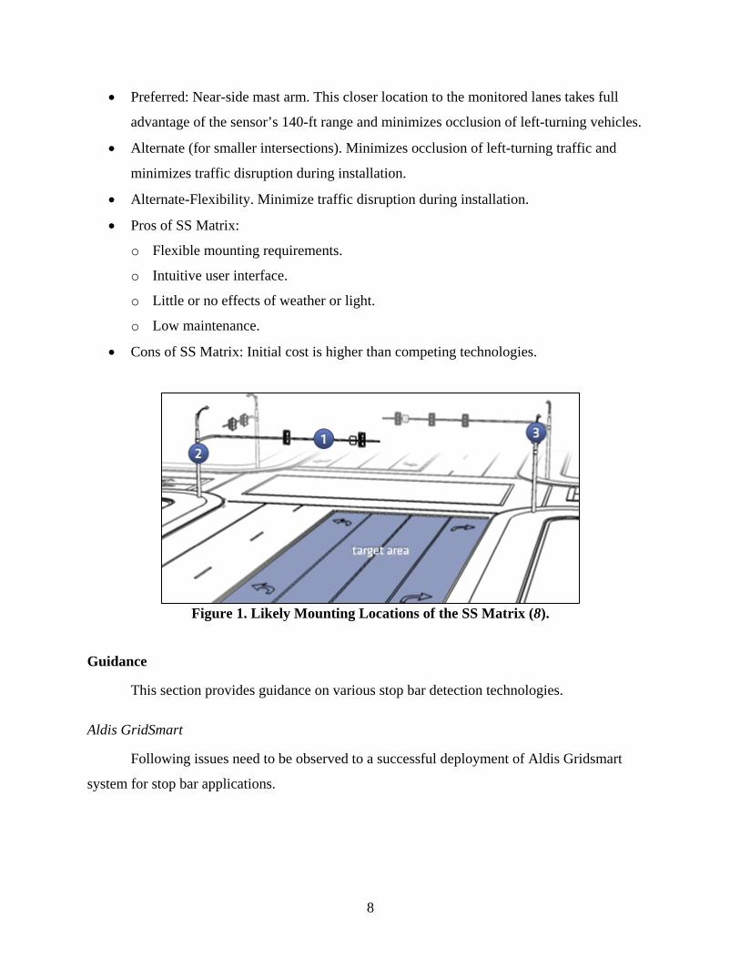
Wavetronix SmartSensor Matrix

The Wavetronix SS Matrix generates 16 separate radar beams to create a 140-ft, 90° field

of view (7, 8). The sensor detects each vehicle within its field of view, knows its position, and

can predict subsequent movements. One strong feature of the SS Matrix is its immunity to

weather and light conditions. The sensor can propagate through rain, snow, fog, or dust storms

without becoming distorted. Figure 1 shows the likely mounting locations for the SS Matrix, and

the preference is as follows:

8

• Preferred: Near-side mast arm. This closer location to the monitored lanes takes full

advantage of the sensor’s 140-ft range and minimizes occlusion of left-turning vehicles.

• Alternate (for smaller intersections). Minimizes occlusion of left-turning traffic and

minimizes traffic disruption during installation.

• Alternate-Flexibility. Minimize traffic disruption during installation.

• Pros of SS Matrix:

o Flexible mounting requirements.

o Intuitive user interface.

o Little or no effects of weather or light.

o Low maintenance.

• Cons of SS Matrix: Initial cost is higher than competing technologies.

Figure 1. Likely Mounting Locations of the SS Matrix (8).

Guidance

This section provides guidance on various stop bar detection technologies.

Aldis GridSmart

Following issues need to be observed to a successful deployment of Aldis Gridsmart

system for stop bar applications.

9

• Camera placement is critical to satisfactory results; daytime false calls are high in left-

turn lanes.

• Monitor performance after installation in all traffic, weather, and light conditions to

determine need for adjustments.

• Check activation times night versus day to determine need for adjustments.

• Excessive outliers could compromise intersection operational efficiency.

Iteris Vantage Vector

Following issues need to be considered to a successful deployment of Iteris Valtage

Vector system for stop bar applications.

• This hybrid is an acceptable and cost-effective solution but not the best for high speeds

(9).

• Mount and aim the video camera like any other video camera then monitor in all traffic,

weather, and light conditions to determine need for adjustments.

• Check video activation times night versus day.

• Motorcycle detection was poor.

Trafficware Pods

Following factors need to be considered for a successful deployment of Trafficware Pods

system for stop bar applications.

• Pods are basically a loop replacement detector with similar characteristics as loops.

• Pods are not likely to be affected by most weather conditions although other research

indicated potential compromise in wireless communication.

• Limit distance of pods and the Access Point to manufacturer recommendations.

• Longitudinal spacing to replicate loops ≤ 12 ft for passenger cars.

• Check sensitivity settings and resulting accuracy using different vehicle types such as

motorcycles and high-bed trucks.

• Check adjacent lane detections.

10

Wavetronix SmartSensor Matrix

Following issues need to be observed to a successful deployment of Wavetronix

SmartSensor Matric system for stop bar applications.

• Consider tall vehicles and possibility of false detections in adjacent lanes.

• Check the impact of stuck-on calls to determine their potential significance.

• Errors might increase in heavy rain and heavy snowfall but not likely in light to moderate

conditions.

• Motorcycle detection is excellent.

UPSTREAM DETECTION

Upstream detectors can be used for sending vehicle information to signal controllers to

prevent vehicles at high-speed intersections to be in their decision zone at the onset of yellow.

They can also be used for extending calls for a phase to service vehicles upstream of the stop bar.

All the detector technologies used for stop bar detection can be used for upstream detections

also. The following list contains some common factors that need to be considered before

selecting a detector technology for upstream detection and how different detectors perform in

these situations:

• High detection accuracy is important to determine when to terminate a phase to prevent

vehicles from being trapped in the decision zone at high-speed intersections. Video

detectors and some of the hybrid detectors have low detection accuracy according to a

TTI study (2). The study found that video camera detectors and Doppler radar (7) have

low detector accuracy upstream of intersection. Also, infrared detectors have a large

number of missed calls during the day but had low missed calls at night. Other detector

technologies with higher detection accuracy should be preferred over these detector

technologies. Wavetronix Advance (SS-200E) uses a Doppler radar with a unique process

for detecting and tracking vehicles. It has high detection accuracy and can be used at

high-speed intersections. Even though it has low classification accuracy, it generally

classifies multiple cars as trucks and does not affect the signal operation adversely.

• For places with high motorcycle volume, Wavetronix Advance (SS-200E) is a good

choice as it has high detection rate for motorcycles. According to a TTI study (2), it had

11

100 percent detection rate for motorcycles. Iteris missed 64.3 percent motorcycles and

Aldis GridSmart (Video camera) has a detection accuracy of 11.3 percent for motorcycles

in the same TTI study.

• Video camera detectors’ detection accuracy decreases during the nighttime. Other

detectors that have a higher nighttime detection accuracy should be considered. Induction

loops, magnetometers, and infrared are not affected by time of day.

• Video camera detectors have unreliable detection rates at high-speed intersections. Other

detectors (induction loops) that have more reliable detection rates should be considered

instead.

Detectors

This section discusses features of the following upstream detectors: Iteris vantage vector

and Wavetronix SS advance.


The Iteris Vantage Vector is a hybrid detector, using both video and radar to enhance

detection. Iteris has offered video detection for many years, but its new detector adds radar to

accomplish enhanced decision zone protection. Additional information provided by the hybrid

sensor includes the number of vehicles, speed, and distance to vehicles in user configurable

zones. Its features include the following (9):

• New graphical-user-interface but maintains familiar video zone setup.

• Wi-Fi connectivity from roadside for laptop, netbook, or iPad.

• Industry standard detection outputs.

• Aesthetic sensor with advanced design and color.

• Video detection to 400 ft.

• Radar detection to 600 ft.

• Vehicle tracking with directional discrimination.

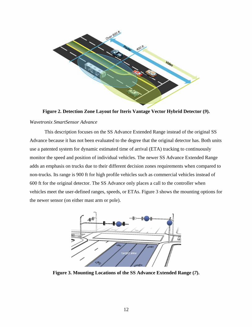
Figure 2 shows the coverage area for the video and radar sensor.

12

Figure 2. Detection Zone Layout for Iteris Vantage Vector Hybrid Detector (9).

Wavetronix SmartSensor Advance

This description focuses on the SS Advance Extended Range instead of the original SS

Advance because it has not been evaluated to the degree that the original detector has. Both units

use a patented system for dynamic estimated time of arrival (ETA) tracking to continuously

monitor the speed and position of individual vehicles. The newer SS Advance Extended Range

adds an emphasis on trucks due to their different decision zones requirements when compared to

non-trucks. Its range is 900 ft for high profile vehicles such as commercial vehicles instead of

600 ft for the original detector. The SS Advance only places a call to the controller when

vehicles meet the user-defined ranges, speeds, or ETAs. Figure 3 shows the mounting options for

the newer sensor (on either mast arm or pole).

Figure 3. Mounting Locations of the SS Advance Extended Range (7).

13

Guidance

This section provides guidance on the upstream detectors.

Aldis GridSmart

Following issues need to be considered when deploying the Aldis Gridsmart system for

advance detection applications:

• Video is not recommended for upstream detection at high-speed intersections.

• If used, monitor performance in all traffic, weather, and light conditions.

• Check false call rate of Aldis upstream camera.

• Rain may affect performance so check during moderate to heavy rain.


Following issues need to be considered when deploying the Iteris Vantage Vector system

for advance detection applications:

• This hybrid detector is a cost-effective solution but not the best for high speeds.

• Missed detections were the most serious problem observed at both triplines on the test

site (2).

• Mount the detector on the near side of the intersection to the approach so it will monitor

at its optimized range.

• This detector is marginal for approaches with high truck volumes near or at 70 mph.

• The detector missed about two-thirds of motorcycles at 50 mph (not tested at 70 mph).

• The Vector provided adequate on times (off minus on) but its activation time was

marginal during rain at 70 mph.

• The installer should test the detector at proposed intersections to determine its vehicle

discovery distance to determine if adding time to the upper end of the range will provide

sufficient protection at green termination.

• Errors in heavy rain and heavy snowfall might increase but not likely in light to moderate

conditions.

14

Trafficware Pods

Following guidelines need to be considered when deploying the Trafficware Pods system

for advance detection applications:

• Detection points for pods will start with TxDOT inductive loop placement based on

design speed and extension times.

• Exact pod placement should consider latency of about 300 milliseconds before and after

vehicles arrive over the pod (2).

• Limit the distance to the farthest pod to not exceed manufacturer recommendations.

Wavetronix SmartSensor Advance (SS-200E)

Following factors need to be considered when deploying the Wavetronix SnmartSensor

system for advance detection applications:

• Set controller extension time to 1.0 second.

• Low measured values of time of arrival of 2.0 to 5.0 seconds need to be verified, but in

the interim, the installer can increase the input values by 0.5 seconds.

• Where feasible, mount the detector on the near side of the intersection.

• In project 0-6828, many non-trucks were classified as trucks, but these errors are not

considered serious. Further research is needed.

• The installer should consider these findings during setup of a new intersection.

• Errors might increase in heavy rain and heavy snowfall but not likely in light to moderate

conditions.

15

CHAPTER 3. DETECTION NEEDS IDENTIFIED BY THE AGENCIES

Researchers contacted officials in the following public agencies to find out the various

detector configuration used in field:

• Fort Worth District.

• Houston District.

• Bryan District.

• Wichita Falls District.

• Corpus Christi District.

• City of Fort Worth.

The section below presents a detailed overview of detection needs for different

approaches based on the response from agencies.

LEFT TURN

The most common technologies used for left turn detection were radars, video detection,

inductive loop, and magnetometers. Many of the new detectors that are installed on left turn

lanes are radar-based detectors. Magnetometer is used at only one site in Houston.

Whenever TxDOT districts in Corpus Christi, Bryan, and some locations in the Fort

Worth District use an induction loop, it is usually between two to three car lengths. This is

usually 40 by 6 ft or 60 by 6 ft. Sometimes the district uses two detectors of 20 by 6 ft with a

6-inch spacing to replicate a 40 by 6 ft loop, as illustrated in Figure 4.

16

20 ft20 ft6 in

6 ft

Detection mode: presenceDelay setting: Used when there is no center median to avoid left turning vehicles from side street to make false calls. Passage setting: 0.5-2 seconds.

40-60 ft

6 ft

Detection mode: presenceDelay setting: 3 second for protected permitted left turns. . Varies with site. Passage setting: 0, 3.5 seconds. Varies with site.

Left Movement – Induction Loops

Figure 4. Typical Left Turn Detector Configuration.

Figure 5 shows the detector configuration used by the City of Fort Worth. The city uses

two detectors for left turns. These detectors are spaced 10 ft apart. The downstream detector is

used for placing calls on a signal controller, and the upstream detector is used to extend the phase

duration.

20 ft20 ft 10 ft

6 ft

Detection mode: presenceDelay Setting: It is used for the second detector from the stop barPassage Setting: 0.5 to 1 seconds

Figure 5. Special Left Turn Detector Configuration.

When video detection is used, the number of detection sections depends on the camera

angle. The detection length is between two and four car lengths. Some intersections in Fort

Worth use a total detection length of two to three car lengths with the detection area consisting of

two zones with a 25-ft overlap. When radar is used, a detection length of approximately 150 ft is

used. This length depends on the location of sensor, angle of the street, and the distance of the

17

zone from the sensor. When magnetometers are used in Houston, 5 to 6 detectors are used to

emulate an induction loop of 40 by 6 ft.

For controller settings, operators at some locations that do not have a median, use delay

setting in the controller to account for left turning vehicles from the cross streets driving over the

left turn detectors and placing a false detector call. The passage time varies between 0 and

3.5 seconds depending on the location and the agency. Some locations increase the passage time

for school events to facilitate an increased number of school buses. Based on the response from

various Texas based agencies, researchers found that detectors in Texas are mainly operated in

presence mode irrespective of type of technology or the turning movement. Also, detector

switching is only used for left turn approaches with permissive left turns.

RIGHT TURN

Right turn detectors have similar detection technology and physical configuration as the

through detectors. Some places provide detectors in right turn bays only for approaches with

high right turn movement. Delay settings for right turns can vary between 5 and 20 seconds

depending upon the location and agency. Passage time for right turning movement is generally

between 0 and 2 seconds. Figure 6 shows a right turn detector configuration.

Right Movement – Induction Loops

40-60 ft

6 ft

6 ft

Detection mode: presenceDelay setting: 8, 20 secondsPassage setting: 0-2 seconds.

20 ft20 ft6 in

Detection mode: presenceDelay setting: 5-7 secondsPassage setting: 0 seconds.

Figure 6. Right Turn Detector Configuration.

18

SLOW-SPEED THROUGH (SPEED<45 MPH)

The physical configuration of detectors for slow speed through movements for agencies

contacted by researchers typically are similar to detector configurations for the left turn

movement detectors. The configuration is characterized by a stop bar detector of 2–3 car lengths

or a pair of detectors with some spacing in between to achieve the same size of detection zone.

Figure 7 shows the through detector configuration.

The Fort Worth District uses a different type of detection configuration, as illustrated in

Figure 8. The configuration only uses an upstream detector, which is used to extend the phase

such that the phase gaps out when the vehicle is between 1–2 seconds from the stop bar.

For controller settings, delay setting is not used for exclusive through movement on

major streets. A delay of 5 seconds is provided in Wichita Falls if the shared lane for through and

right turns is present. The City of Fort Worth use the delay duration on minor streets. It varies by

time of day to provide snappier operations during the day and less snappy operations during the

night. A typical value of delay for night time is between 10 and 15 seconds. Passage time

between 0 and 4.5 seconds is used.

HIGH-SPEED THROUGH (SPEED>45 MPH)

Most of the places use radar-based detection at upstream locations for high-speed

intersections. Wichita Falls is the only exception that used video detectors. Fort Worth uses the

typical TxDOT guidance on placement of detectors for upstream detection. The stop bar

detection technology and physical configuration is similar to slow-speed through movements.

Upstream detection zone position and length is based on the decision zone. Generally, the

upstream detection zone is between 2.5 and 5.5 seconds from the stop bar. In Fort Worth, the

detection zone is between 2.5 and 6 seconds from the stop bar. The position of upstream

detection zone also depends on the approach speed at an intersection. Fort Worth uses a passage

time of 0.1 and 0.5 seconds. Wichita Falls uses a passage time of 3.5 seconds. Figure 9 shows a

high-speed intersection detector configuration being used by the Fort Worth District.

19

Through Movement (Speed<45 mph) Induction Loops

40-60 ft

20 ft20 ft6 in

6 ft

6 ft

Detection mode: presenceDelay setting: 5 seconds (free right turns only). Only provided when shared through and right lane present. Passage setting: 0, 3.5 seconds. Site dependent.

Detection mode: presenceDelay setting: Generally none. Cross street delay depends on time of day. Night time delay can be between 10 and 15 seconds. Passage setting: 0-4.5 seconds. Site dependent.

Figure 7. Through Detector Configuration.

Through Movement (Speed<45 mph) Induction Loops

6 ft

Major StreetDetection mode: presenceDelay Setting: nonePassage Setting: 2 seconds

250-300 ft6 ft

6 ft

Minor StreetDetection mode: presenceDelay Setting: nonePassage Setting: 1.0 to 1.5 seconds

120 ft6 ft

Figure 8. Fort Worth District Through Detector Configuration for Slow Speeds.

20

Upstream detector

2.5 seconds

Houston, Fort Worth

Detection mode: presencePassage setting: 0.1 to 0.5 seconds

5.5-6 seconds

High speed intersections- Upstream radar detectors

Figure 9. High-Speed Intersection Detector Configuration.

21

CHAPTER 4. DETECTOR APPLICABILITY BY TURNING MOVEMENT

Researchers identified various manners in which the application/detector needs can be

met by different detection technology. In most cases, multiple technologies are identified with

each having its own design, configuration, and implementation.

LEFT AND RIGHT TURN

The most common detector configuration used in left turn bays was a detection zone that

was 6-ft wide and usually 40 to 60 ft in length, as shown in Figure 4. This is usually to

accommodate two to three car lengths within the detection zone. This detection zone

configuration can be implemented using various detection technologies. The simplest way to

implement the detector layout is done by using inductive loops as illustrated in the handbook.

The same detector layout can also be implemented using a video detection system as illustrated

in the handbook and illustrated in Figure 10.

Some districts and other operating agencies have also started using magnetometers for

vehicle detection at a few locations. Magnetometers have the advantage of inductive loops

without the intrusive large saw cuts, conduits, and cables running over long distance. Modern

magnetometers have improved the range to about 900 ft very accurately and have simplified the

installation and configuration to make it more practical in modern signal controller cabinets.

Each magnetometer has a detection zone in the shape of a circle of a radius of approximate 3 ft

simulating a 6 × 6 loop. Multiple magnetometers are installed about 6 ft apart and configured to a

single channel to emulate a stop bar detector of 6 × 40 ft, as illustrated in Figure 11.

Stop bar detection is also implemented using radar detection. Figure 12 shows the

positions for radar detector installation. It is installed either on a corner of the intersection on

signal pole, illustrated as Position A and Position B or on a mast arm (Position C). The radar

range is an arc of 90°. Proper positioning of the radar detector can improve the accuracy of

detection. Position A and Position C are more accurate for detecting vehicles in the left lane as

there is minimal occlusion.

Figure 5 shows the detector configuration used by City of Fort Worth. The city uses two

detectors for left turns. These detectors are spaced 10 ft apart. The downstream detector is used

for placing calls on a signal controller and upstream detector is used to extend the phase

duration.

22

Figure 10. Stop Bar Detector Configuration Using Video Detection.

40-60 ft

6 ft

Figure 11. Use of Magnetometers to Emulate a Stop Bar Detector.

23

Position A Position B

Position C

Figure 12. Stop Bar Detector Configuration Using Radar.

Operating agencies can use any of the above mentioned technologies to configure

detectors to detect vehicles in the left turn bay. However, engineers can choose the appropriate

technology based on the desired operational configuration (i.e., number of required channels,

accuracy thresholds, and acceptable sensitivity). Sensitivity is measured as a variability of the

size of the detection zone based on detector installation, size of the detector, and the size of the

vehicle. As shown in Figure 13, when a technology like video detection is used to configure

detection zones A, B, and C, the effective detection zones depend on the vehicle. As shown in

the figure, even though a car leaves the designed detection zone C, it is still detected and obtains

a much larger effective detection zone. This zone becomes considerably larger for a larger

vehicle like a bus, resulting in one continuous detection zone. If efficiency is a high priority, the

size of the detection zone being consistent is crucial. Engineers have to evaluate the available

technologies and select the appropriate one to suit the operational objectives.

24

C

Zone A Zone B Zone CDesigned Detection

Zone C

Effective Detection Zone C for a Car

Effective Detection Zone for a Bus

Figure 13. Impact of Technology on Effective Detection Zones.

SLOW-SPEED THROUGH (SPEED<45 MPH)

Detection configuration for through movements for lower speeds is very similar to the

configurations for left turn movements. Video detection technology as illustrated in Figure 10,

magnetometers as illustrated in Figure 11, and radar detection as illustrated in Figure 12 are

applicable for through movements. The City of Fort Worth uses a different type of detection

configuration as illustrated in Figure 8. The configuration only uses an upstream detector that is

used to extend the phase such that the phase gaps out when the vehicle is between 1–2 seconds

from the stop bar.

However, such a configuration warrants a technology that detects the vehicles precisely

to ensure the effective detection zone is very close to the design detection. Properly adjusted

inductive loops and magnetometers can serve as the appropriate detection technology for this

configuration.

HIGH-SPEED THROUGH (SPEED>45 MPH)

Most of the places use radar-based detection at upstream locations for high-speed

intersections. Wichita Falls is the only exception that used video detectors. Fort Worth uses the

typical TxDOT guidance on placement of detectors for upstream detection. The stop bar

detection technology and physical configuration is similar to slow-speed through movements.

Upstream detection zone position and length is based on the decision zone requirements.

Generally, the upstream detection zone is between 2.5 and 5.5 seconds from the stop bar. In

Fort Worth, the detection zone is between 2.5 and 6 seconds from the stop bar. The position of

25

upstream detection zone also depends on the approach speed at an intersection. Fort Worth uses a

passage time of 0.1 and 0.5 seconds. Wichita Falls uses a passage time of 3.5 seconds. Figure 9

shows the configuration of radar detector for high-speed intersection detectors.

Election of proper technology is essential to ensure that the implemented detection

technology fits the design for the high-speed approaches. Currently the suitable technologies

include inductive loops, radar, and magnetometer detection system illustrated in Figure 14.

d3d2

d1

Magnetometers

Figure 14. Use of Magnetometers for High-Speed Approaches.

27

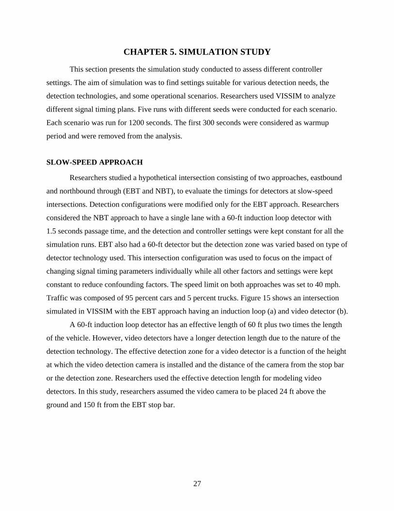
CHAPTER 5. SIMULATION STUDY

This section presents the simulation study conducted to assess different controller

settings. The aim of simulation was to find settings suitable for various detection needs, the

detection technologies, and some operational scenarios. Researchers used VISSIM to analyze

different signal timing plans. Five runs with different seeds were conducted for each scenario.

Each scenario was run for 1200 seconds. The first 300 seconds were considered as warmup

period and were removed from the analysis.

SLOW-SPEED APPROACH

Researchers studied a hypothetical intersection consisting of two approaches, eastbound

and northbound through (EBT and NBT), to evaluate the timings for detectors at slow-speed

intersections. Detection configurations were modified only for the EBT approach. Researchers

considered the NBT approach to have a single lane with a 60-ft induction loop detector with

1.5 seconds passage time, and the detection and controller settings were kept constant for all the

simulation runs. EBT also had a 60-ft detector but the detection zone was varied based on type of

detector technology used. This intersection configuration was used to focus on the impact of

changing signal timing parameters individually while all other factors and settings were kept

constant to reduce confounding factors. The speed limit on both approaches was set to 40 mph.

Traffic was composed of 95 percent cars and 5 percent trucks. Figure 15 shows an intersection

simulated in VISSIM with the EBT approach having an induction loop (a) and video detector (b).

A 60-ft induction loop detector has an effective length of 60 ft plus two times the length

of the vehicle. However, video detectors have a longer detection length due to the nature of the

detection technology. The effective detection zone for a video detector is a function of the height

at which the video detection camera is installed and the distance of the camera from the stop bar

or the detection zone. Researchers used the effective detection length for modeling video

detectors. In this study, researchers assumed the video camera to be placed 24 ft above the

ground and 150 ft from the EBT stop bar.

28

EBT

EBT

a) Induction Loop Detector b) Video Detector Figure 15. VISSIM Network for Single Lane EBT Approach.

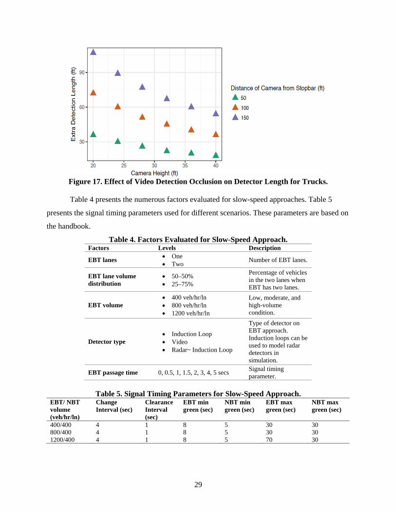
Figure 16 and Figure 17 illustrate the increase in the detection length for cars and trucks

for various camera heights and distances from stop bar. The effective detector length is longer

when camera height is low and distance of camera from the stop bar is large.

Figure 16. Effect of Video Detection Occlusion on Detector Length for Cars.

29

Figure 17. Effect of Video Detection Occlusion on Detector Length for Trucks.

Table 4 presents the numerous factors evaluated for slow-speed approaches. Table 5

presents the signal timing parameters used for different scenarios. These parameters are based on

the handbook.

Table 4. Factors Evaluated for Slow-Speed Approach. Factors Levels Description

EBT lanes • One • Two Number of EBT lanes.

EBT lane volume distribution

• 50–50% • 25–75%

Percentage of vehicles in the two lanes when EBT has two lanes.

EBT volume • 400 veh/hr/ln • 800 veh/hr/ln • 1200 veh/hr/ln

Low, moderate, and high-volume condition.

Detector type • Induction Loop • Video • Radar~ Induction Loop

Type of detector on EBT approach. Induction loops can be used to model radar detectors in simulation.

EBT passage time 0, 0.5, 1, 1.5, 2, 3, 4, 5 secs Signal timing parameter.

Table 5. Signal Timing Parameters for Slow-Speed Approach.

EBT/ NBT volume (veh/hr/ln)

Change Interval (sec)

Clearance Interval (sec)

EBT min green (sec)

NBT min green (sec)

EBT max green (sec)

NBT max green (sec)

400/400 4 1 8 5 30 30 800/400 4 1 8 5 30 30 1200/400 4 1 8 5 70 30

30

Researchers measured the following performance measures during the simulation study:

• Average delay and queue for the two approaches and the intersection.

• Average residual queue at the end of EBT and NBT phase.

• Percentage of max-outs.

HIGH-SPEED APPROACH

Signal timing for high-speed approach was evaluated using the intersection described in

the previous section with some minor differences. EBT approach had two lanes with 60 mph

speed limit. Researchers evaluated three EBT volumes: 400, 800, and 1200 veh/hr/ln. High-

speed approaches with advanced induction loops and radar detectors was studied. The inductive

loop configuration was used as the baseline for comparing the other technologies A 40-ft stop

bar detector and three upstream detectors at 275, 375, and 475 ft were used when induction loops

were used on EBT approach. Two detector configuration options were evaluated for induction

loop. In one case, the stop bar and upstream detector were on the same channel. The second

scenario consisted of the stop bar and upstream detectors on separate channels. These detector

configurations are based on the handbook. For radar detector, researchers modeled two

configurations: Radar 1 and Radar 2. Radar 1 detection zone consisted of an upstream detection

area between 2.5 and 5.5 seconds from the stop bar (decision zone) and a 40-ft stop bar detector.

Radar 2 detector configuration consisted of two 6-ft detectors at 355 and 485 ft from the stop bar

and a 40-ft detector at the stop bar. The stop bar and upstream detections were sent on separate

channels. Figure 18 and Figure 19 show the configuration for Radar 1 and Radar 2, respectively.

Following passage times were evaluated:

• Induction loop with all detections on same channel: 1.1, 1.5, 1.8, 2.5, 3, and 5 seconds.

• Induction loop with stop bar detector on separate channel: 2 seconds for stop bar detector.

1.1, 1.5, 1.8, 2.5, 3, and 5 seconds for upstream detectors.

• Radar 1: 2 seconds for the stop bar detector: 0.5, 0.9, 1.2, 1.9, 2.4, and 4.4 seconds for

upstream detectors.

• Radar 2: 1.8 seconds for the stop bar detector and 1.8 seconds for the upstream detectors.

31

Upstream detector

2.5 seconds

Detection mode: presenceUpstream detector passage time: 0.5, 0.9, 1.2, 1.9, 2.4 and 4.4 secondsStop bar detector passage time: 1.8 seconds

5.5 seconds

40 ft

Figure 18. Detector Configuration for Radar 1.

4 seconds

Detection mode: presenceUpstream detector passage time: 1.8 secondsStop bar detector passage time: 1.8 seconds

5.5 seconds

40 ft

6 ft

Figure 19. Detector Configuration for Radar 2.

Table 6 shows the signal timing parameters for different volumes. The passage time for

upstream detection for Radar 1 is 0.6 second less than the passage times for induction loop with

advanced detectors on separate channel. A 0.6 second offset is needed to find equivalent

scenarios. The offset considers the travel time to the stop bar at 60 mph from the closest

upstream induction loop detector (3.1 seconds) and Radar 1 (2.5 seconds). Researchers obtained

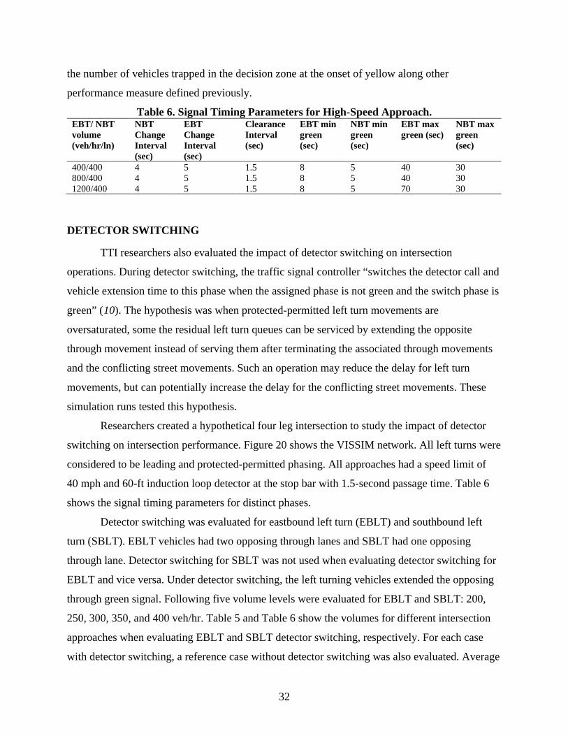
32

the number of vehicles trapped in the decision zone at the onset of yellow along other

performance measure defined previously.

Table 6. Signal Timing Parameters for High-Speed Approach. EBT/ NBT volume (veh/hr/ln)

NBT Change Interval (sec)

EBT Change Interval (sec)

Clearance Interval (sec)

EBT min green (sec)

NBT min green (sec)

EBT max green (sec)

NBT max green (sec)

400/400 4 5 1.5 8 5 40 30 800/400 4 5 1.5 8 5 40 30 1200/400 4 5 1.5 8 5 70 30

DETECTOR SWITCHING

TTI researchers also evaluated the impact of detector switching on intersection

operations. During detector switching, the traffic signal controller “switches the detector call and

vehicle extension time to this phase when the assigned phase is not green and the switch phase is

green” (10). The hypothesis was when protected-permitted left turn movements are

oversaturated, some the residual left turn queues can be serviced by extending the opposite

through movement instead of serving them after terminating the associated through movements

and the conflicting street movements. Such an operation may reduce the delay for left turn

movements, but can potentially increase the delay for the conflicting street movements. These

simulation runs tested this hypothesis.

Researchers created a hypothetical four leg intersection to study the impact of detector

switching on intersection performance. Figure 20 shows the VISSIM network. All left turns were

considered to be leading and protected-permitted phasing. All approaches had a speed limit of

40 mph and 60-ft induction loop detector at the stop bar with 1.5-second passage time. Table 6

shows the signal timing parameters for distinct phases.

Detector switching was evaluated for eastbound left turn (EBLT) and southbound left

turn (SBLT). EBLT vehicles had two opposing through lanes and SBLT had one opposing

through lane. Detector switching for SBLT was not used when evaluating detector switching for

EBLT and vice versa. Under detector switching, the left turning vehicles extended the opposing

through green signal. Following five volume levels were evaluated for EBLT and SBLT: 200,

250, 300, 350, and 400 veh/hr. Table 5 and Table 6 show the volumes for different intersection

approaches when evaluating EBLT and SBLT detector switching, respectively. For each case

with detector switching, a reference case without detector switching was also evaluated. Average

33

delay and queue length on EBLT, EBT, westbound through (WBT), and entire intersection were

analyzed for EBLT detector switching. Average delay and queue length on SBLT, southbound

through (SBT), NBT, and entire intersection were analyzed for SBLT detector switching.

EBT

Figure 20. VISSIM Network for Evaluating Detector Switching.

Table 7. Signal Timing Parameters for Detector Switching Scenarios. Movement Min

green (sec)

Change interval (sec)

Clearance interval (sec)

Max green (sec)

EBT 8 4 1 30 EBLT 5 4 1 18 WBT 8 4 1 30 WBLT (westbound left turn) 5 4 1 18 NBT 5 4 1 30 NBLT (northbound left turn) 5 4 1 15 SBT 5 4 1 30 SBLT (southbound left turn) 5 4 1 15

Table 8. Movement Volumes – EBLT Detector Switching. EBT EBLT WBT WBLT 800 veh/hr Varies 800 veh/hr 150 veh/hr NBT NBLT SBT SBLT 400 veh/hr 150 veh/hr 400 veh/hr 150 veh/hr

Table 9. Movement Volumes – SBLT Detector Switching. EBT EBLT WBT WBLT 800 veh/hr 150 veh/hr 800 veh/hr 150 veh/hr NBT NBLT SBT SBLT 400 veh/hr 150 veh/hr 400 veh/hr Varies

34

MAXIMUM GREEN TIME

This study compared the impact of different maximum green time on intersection

performance. Researchers studied a hypothetical intersection consisting of only two approaches,

eastbound and northbound through (EBT and NBT), to evaluate the timings for detectors at

slow-speed intersections. Detection configurations were modified only for the EBT approach.

Researchers considered the NBT approach to have a single lane with a 60-ft induction loop

detector with 1.5 seconds passage time, and the detection and controller settings were kept

constant for all the simulation runs. EBT also had a 60-ft induction loop detector. This

intersection configuration was used to focus on the impact of changing signal timing parameters

individually while all other factors and settings were kept constant to reduce confounding

factors. The speed limit on both approaches was set to 40 mph. Traffic was composed of

95 percent cars and 5 percent trucks. Figure 21 shows the intersection simulated in VISSIM.

Figure 21. VISSIM Network for Evaluating Maximum Green Times.

The NBT and EBT maximum green time for the base case were determined using the

handbook. The maximum green time for NBT was 30 seconds. EBT maximum green time was

40 and 70 seconds for moderate and high volume, respectively. EBT maximum green time was

increased by 5 and 10 seconds to understand the impact of maximum green time on intersection

performance. Table 10 shows the factors evaluated for this study. Researchers created 72

scenarios based on the combination of these factors. Intersection operations are not impacted by

maximum green time at low volumes, so low volume scenarios were not simulated.

35

Table 10. Factors Evaluated for Studying Maximum Green Time. Factors Variables Description EBT lane volume distribution

• 50–50% • 25-75%

Percentage of vehicles in the two lanes when EBT has two lanes

Volumes Levels • 800 veh/hr/lane • 1200 veh/hr/lane

Moderate and high-volume condition

Passage Times (seconds) 1.0., 1.5, 2.0, 3.0, 4.0, and 5.0 Signal timing parameter

Maximum green time

• Max green time by Traffic signal operation handbook

• +5 seconds • + 10 seconds

Maximum green time for EBT

SIMULTANEOUS GAP OUTS

The traffic signal timing manual defines the simultaneous gap as “all phases that are

timing concurrently to simultaneously reach a point of being committed to terminate (by gap-out,

max-out, or force-off) before they can be allowed to jointly terminate. If disabled, each of the

concurrent phases can reach a point of being committed to terminate separately and remain in

that state while waiting for all concurrent phases to achieve this status” (11).

This study compared the performance of high-speed intersections with and without

simultaneous gap outs on high-speed approaches. The study network consists of three

approaches: EBT, WBT, and NBT. Simultaneous and non-simultaneous gap out settings are

implemented on the EBT and WBT directions. EBT and WBT approaches have two lanes with a

60 mph speed limit, an upstream radar detector, and a 40-ft stop bar detector. NBT has a 60-ft

induction loop with 1.5-second passage time and speed limit of 40 mph. Traffic was composed

of 95 percent cars and 5 percent trucks.

Table 11 presents the factors evaluated. Nine combinations of high-speed approach

volumes were considered. A previous study on high-speed intersection showed that the passage

time of 0.5 second provided the best performance among all passage times, so a 0.5-second

passage time is used. There are nine scenarios with simultaneous gap on the high-speed approach

and nine without simultaneous gap on the high-speed approach.

36

Figure 22. VISSIM Network for Evaluating Simultaneous Gap.

Table 11. Factors Evaluated for Studying Simultaneous Gap. Factors Variables Description

Volumes Levels EBT • 400 veh/hr/lane • 800 veh/hr/lane • 1200 veh/hr/lane

Low, moderate and high volume condition

Volumes Levels WBT • 400 veh/hr/lane • 800 veh/hr/lane • 1200 veh/hr/lane

Low, moderate and high volume condition

Passage Times (seconds) • 0.5 seconds Signal timing

parameter

Gap out • Simultaneous • Non-Simultaneous

Type of gap out setting

37

CHAPTER 6. RESULTS

This section presents the results for the simulation studies described in the previous

chapter.

SLOW-SPEED APPROACH

As described in earlier chapters, TTI researchers assessed the impact of volumes on the

major street, number of lanes on the major street (EBT), lane distribution, detector types, and

passage times on the average delay for major street (EBT), minor street (NBT), and overall

intersection. Figure 23 and Figure 24 illustrate the results of this analysis. Average intersection

delay stays almost constant with an increase in passage time at low volumes. There is a slight

decrease in the major street average delay. However, the minor street delay increases sharply

with the increase in major street passage time at higher volumes. Average delay patterns for

induction loop and video detectors are similar across different factors. Thus, type of detectors

does not have a significant impact on performance when an intersection has low demand.

Figure 23. Average Delay for Slow-Speed Approaches – Single Lane EBT.

38

Figure 24. Average Delay for Slow-Speed Approaches – Two Lane EBT.

Average delay during the moderate volumes is similar to the average delay during low

volumes for the single-lane approach and the two-lane approach with equal volume distribution.

The average delay for the intersection and major street approach is higher when the major street

has an unequal distribution of vehicles on the two lanes. A passage time between 1 and 2 seconds

was found to be optimal based on delay experienced on the major street, minor street, and overall

intersection. When considering detection technology, video detectors in most scenarios

illustrated lower average intersection delay as compared to induction loop for the same passage

time. This implied that the length of detection zone needs to be considered when using lower

passage times.

The choice of passage time is crucial for managing delay at an intersection with high

volume. Tests indicated that a larger passage time on major street phases cause an increase in the

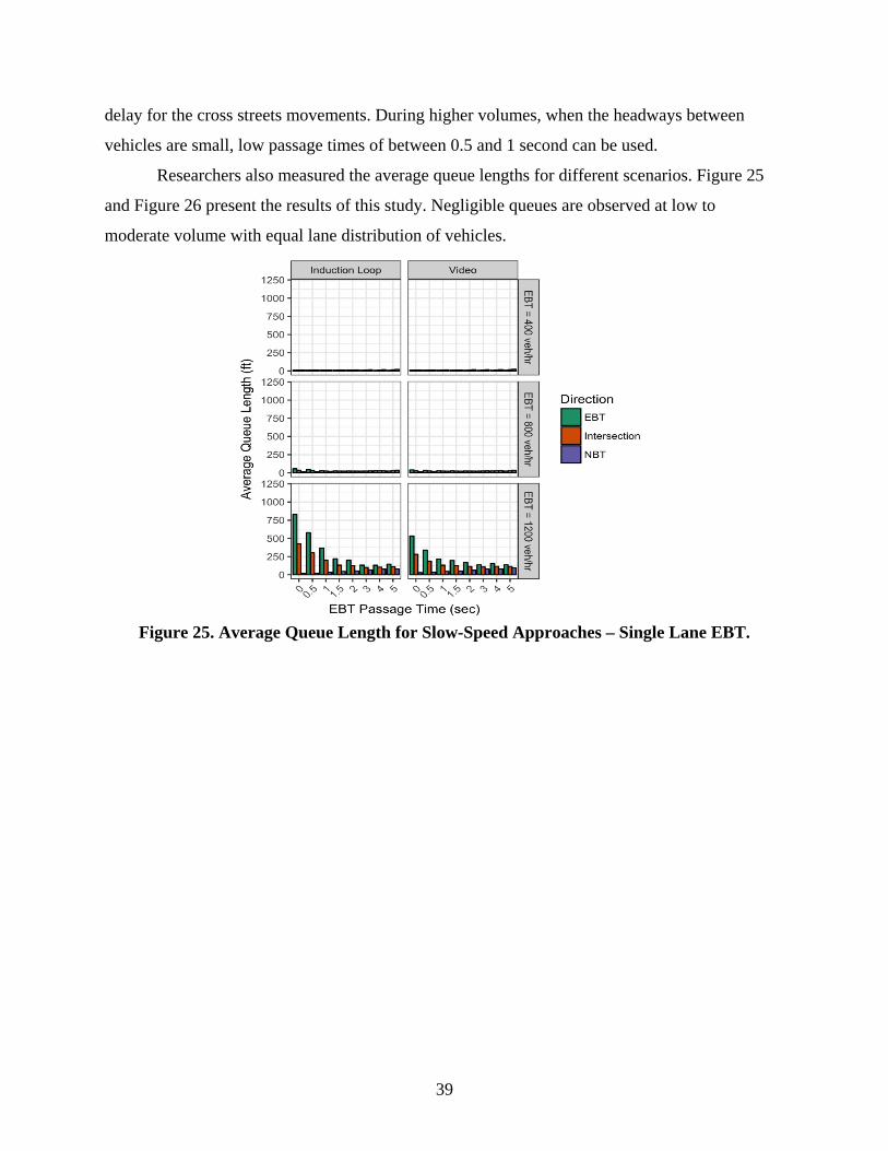
39

delay for the cross streets movements. During higher volumes, when the headways between

vehicles are small, low passage times of between 0.5 and 1 second can be used.

Researchers also measured the average queue lengths for different scenarios. Figure 25

and Figure 26 present the results of this study. Negligible queues are observed at low to

moderate volume with equal lane distribution of vehicles.

Figure 25. Average Queue Length for Slow-Speed Approaches – Single Lane EBT.

40

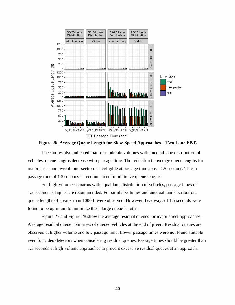
Figure 26. Average Queue Length for Slow-Speed Approaches – Two Lane EBT.

The studies also indicated that for moderate volumes with unequal lane distribution of

vehicles, queue lengths decrease with passage time. The reduction in average queue lengths for

major street and overall intersection is negligible at passage time above 1.5 seconds. Thus a

passage time of 1.5 seconds is recommended to minimize queue lengths.

For high-volume scenarios with equal lane distribution of vehicles, passage times of

1.5 seconds or higher are recommended. For similar volumes and unequal lane distribution,

queue lengths of greater than 1000 ft were observed. However, headways of 1.5 seconds were

found to be optimum to minimize these large queue lengths.

Figure 27 and Figure 28 show the average residual queues for major street approaches.

Average residual queue comprises of queued vehicles at the end of green. Residual queues are

observed at higher volume and low passage time. Lower passage times were not found suitable

even for video detectors when considering residual queues. Passage times should be greater than

1.5 seconds at high-volume approaches to prevent excessive residual queues at an approach.

41

Figure 27. Average Residual Queue Length for Slow-Speed Approaches – Single Lane

EBT.

Figure 28 shows the average residual queues on the major street for slow-speed

approaches on a multilane approach with balanced and unbalanced lane distribution. While some

residual queues were observed for uneven lane distribution at moderate volumes levels, much

larger queues were observed for the high-volume scenarios. This indicates max time used for

high-volume approaches having equal distribution of vehicles across lanes is not enough when

the vehicle distribution across lanes is not uniform. Moreover, passage time should be greater

than 1.5 seconds at high-volume approaches to prevent excessive residual queues at an approach.

42

Figure 28. Average Residual Queue Length for Slow-Speed Approaches – Two Lane EBT.

Figure 29 and Figure 30 illustrate the percent max-outs for the major street approaches.

The simulation results indicated that probability of max-outs increased with passage times

greater than 1.5 to 2 seconds with a slightly higher percentage for video detection compared to

inductive loops for single-lane approaches. These percentages increased significantly for the

two-lane approach case. Max-outs need to be monitored at moderate to high-volume approaches

with multiple lanes. Large numbers of max-outs indicate either that the demand on that approach

is being met thus max green needs to be increased or the passage time needs to be decreased to

make the operation snappier.

43

Figure 29. EBT Max-Outs for Slow-Speed Approaches – Single Lane EBT.

44

Figure 30. Max-Outs for Slow-Speed Approaches – Two Lane EBT.

The above results show that finding an optimal timing plan is a multi-objective

optimization problem. Average delay, queue lengths, residual queues, and max-outs need to be

considered simultaneously to choose signal controller parameters. In general, smaller passage

time for an approach reduces max-outs but increases the residual queues, delay, and queue length

for that approach and the intersection. Passage time between 1.5 and 2 seconds are optimal when

considering the above four criteria.

HIGH-SPEED APPROACH

Figure 31 illustrates average delay experienced on a high-speed approach with different

detection configurations and technologies. Under lower to moderate volume conditions,

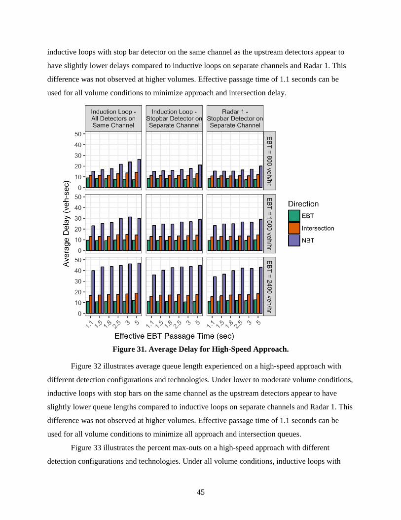
45

inductive loops with stop bar detector on the same channel as the upstream detectors appear to

have slightly lower delays compared to inductive loops on separate channels and Radar 1. This

difference was not observed at higher volumes. Effective passage time of 1.1 seconds can be

used for all volume conditions to minimize approach and intersection delay.

Figure 31. Average Delay for High-Speed Approach.

Figure 32 illustrates average queue length experienced on a high-speed approach with

different detection configurations and technologies. Under lower to moderate volume conditions,

inductive loops with stop bars on the same channel as the upstream detectors appear to have

slightly lower queue lengths compared to inductive loops on separate channels and Radar 1. This

difference was not observed at higher volumes. Effective passage time of 1.1 seconds can be

used for all volume conditions to minimize all approach and intersection queues.

Figure 33 illustrates the percent max-outs on a high-speed approach with different

detection configurations and technologies. Under all volume conditions, inductive loops with

46

stop bars on the same channel as the upstream detectors appear to have a slightly higher percent

of max-outs compared to inductive loops on separate channels and Radar 1. Radar 1 and

induction loops on separate channels perform better than induction detectors with all detectors on

the same channel.

Figure 32. Average Queue Length – High-Speed Approach.

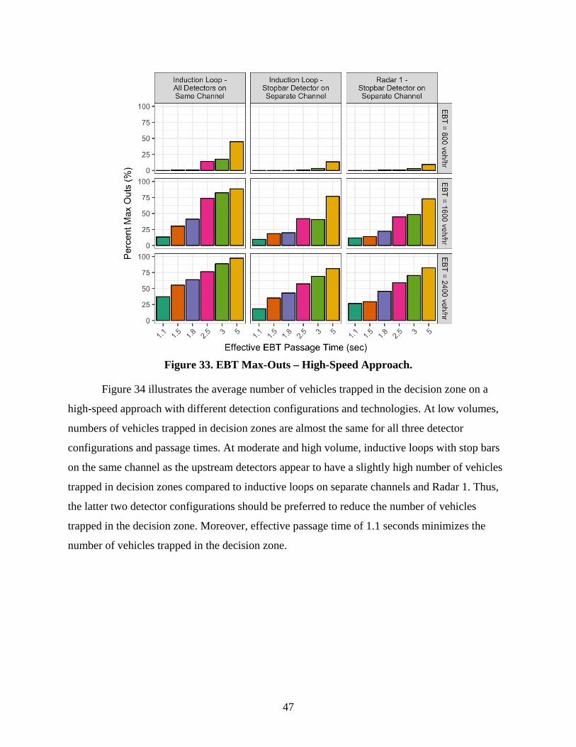
47

Figure 33. EBT Max-Outs – High-Speed Approach.

Figure 34 illustrates the average number of vehicles trapped in the decision zone on a

high-speed approach with different detection configurations and technologies. At low volumes,

numbers of vehicles trapped in decision zones are almost the same for all three detector

configurations and passage times. At moderate and high volume, inductive loops with stop bars

on the same channel as the upstream detectors appear to have a slightly high number of vehicles

trapped in decision zones compared to inductive loops on separate channels and Radar 1. Thus,

the latter two detector configurations should be preferred to reduce the number of vehicles

trapped in the decision zone. Moreover, effective passage time of 1.1 seconds minimizes the

number of vehicles trapped in the decision zone.

48

Figure 34. Number of Vehicles Trapped in Decision Zone – High-Speed Approach.

The above results show that Radar 1 and induction loop detectors with detectors on

separate channel are preferable at high-speed approaches. Moreover, 1.1-second effective

passage time (0.5 seconds for Radar 1) provide the best performance in terms of max-outs,

average delay, average queue length, and number of vehicles trapped in decision zone.

The average delay, queue length, max-outs, and number of vehicles trapped in decision

zones were similar for both radar detectors. Figure 35 and Figure 36 show the max-outs and

number of vehicles trapped in the decision zone for Radar 1 and Radar 2. Percent of max-outs

are lower for Radar 1 for any given volume level. Numbers of vehicles trapped in decision zones

are similar for both the detectors when Radar 2 has a passage time of 1.8 seconds, and Radar 1

has a passage time of 0.5 seconds for the upstream detector.

49

Figure 35. EBT Max-Outs – Radar 1 and Radar 2.

Figure 36. Number of Vehicles Trapped in Decision Zone – Radar 1 and Radar 2.

50

DETECTOR SWITCHING

Figure 37 and Figure 38 illustrate the delays experienced when detector switching was

implemented for EBLT turning vehicles turning across two through lanes. Figure 39 and Figure

40 illustrate the delays experienced when detector switching was implemented for SBLT

vehicles turning across a single through lane. Detector switching was successful in reducing the

delay and queues on the left turning approach when there are two opposing lanes.

Figure 37. Average Delay – EBLT Detector Switching.

Figure 38. Average Queue – EBLT Detector Switching.

51

Figure 39. Average Delay – SBLT Detector Switching.

Figure 40. Average Queue – SBLT Detector Switching.

MAXIMUM GREEN TIME

Figure 41 shows the percentage of max-outs for different scenarios. In the figure, Traffic

Signal Operations handbook (TSOH(1)) represents the maximum green time obtained from the

handbook; plus5 and plus10 are the maximum green times obtained by adding 5 and 10 seconds

to the maximum green time obtained from the handbook. At moderate volume, EBT max-outs

decrease with an increase in EBT maximum green time by both 5 seconds and 10 seconds. At

higher volume, the reduction in EBT max-outs mainly occurs when the maximum green time is

increased by 10 seconds.

52

Figure 42 and Figure 43 show the average delay and queue for EBT, NBT and

intersections under different conditions. Increasing the maximum green time has little effect on

the average delay and queues for the EBT approach and the entire intersection.

Figure 41. Max-Outs – Maximum Green Times.

53

Figure 42. Average Delay – Maximum Green Times.

Figure 43. Average Queue – Maximum Green Times.

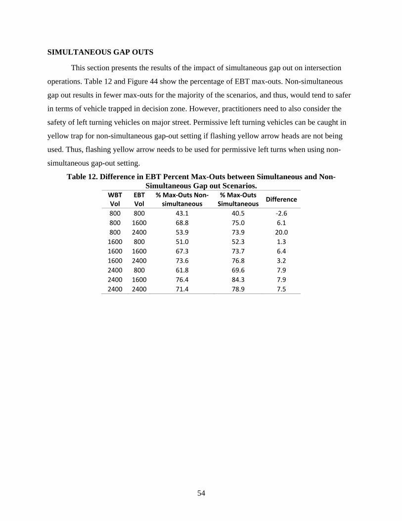
54

SIMULTANEOUS GAP OUTS

This section presents the results of the impact of simultaneous gap out on intersection

operations. Table 12 and Figure 44 show the percentage of EBT max-outs. Non-simultaneous

gap out results in fewer max-outs for the majority of the scenarios, and thus, would tend to safer

in terms of vehicle trapped in decision zone. However, practitioners need to also consider the

safety of left turning vehicles on major street. Permissive left turning vehicles can be caught in

yellow trap for non-simultaneous gap-out setting if flashing yellow arrow heads are not being

used. Thus, flashing yellow arrow needs to be used for permissive left turns when using non-

simultaneous gap-out setting.

Table 12. Difference in EBT Percent Max-Outs between Simultaneous and Non-Simultaneous Gap out Scenarios.

WBT Vol

EBT Vol

% Max-Outs Non-simultaneous

% Max-Outs Simultaneous Difference

800 800 43.1 40.5 -2.6 800 1600 68.8 75.0 6.1 800 2400 53.9 73.9 20.0

1600 800 51.0 52.3 1.3 1600 1600 67.3 73.7 6.4 1600 2400 73.6 76.8 3.2 2400 800 61.8 69.6 7.9 2400 1600 76.4 84.3 7.9 2400 2400 71.4 78.9 7.5

55

Figure 44. Max-Outs – Simultaneous vs. Non-simultaneous Gap.

Table 13 and Figure 45 shows the number of vehicles trapped in the decision zone in

EBT approach. Number of vehicle trapped in the decision zone are similar for Simultaneous and

non-simultaneous gap out scenarios. Simultaneous gap settings can have some effect in

decreasing the number of vehicles trapped in the decision zone when both high-speed approaches

have low volumes (800 veh/hr). Researchers also found that simultaneous gap setting does not

have an effect on overall intersection delay or queue.

Table 13. Vehicles Trapped in Decision Zone.

WBT Vol EBT Vol Veh in Decision Zone(veh/cycle) Non- Simultaneous

Veh in Decision Zone(veh/cycle) Simultaneous

Difference

800 800 1.38 1.27 -0.11 800 1600 2.19 2.27 0.08 800 2400 2.54 3.11 0.57

1600 800 1.78 1.98 0.20 1600 1600 2.50 2.65 0.15 1600 2400 3.38 3.45 0.08 2400 800 2.67 2.58 -0.09 2400 1600 3.51 3.27 -0.24 2400 2400 3.92 4.47 0.55

56

Figure 45. Number of Vehicles Trapped in Indecision Zone – Simultaneous vs. Non-

simultaneous Gap.

SUMMARY

The following observations were made for slow-speed through approaches at a 40 mph

speed limit:

• Low-Volume Scenarios:

o 0-second passage times provide snappier operations and minimize delay for all

approaches and the intersection.

o Negligible queues were found at major streets, minor streets, and intersections for all

passage times.

o Similar performance was observed for both induction loop and video detectors.

• Moderate-Volume Scenarios:

o Smaller passage times can be used when major street lanes have equal distribution of

vehicles.

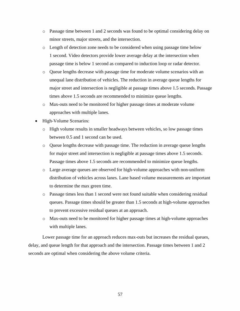
57

o Passage time between 1 and 2 seconds was found to be optimal considering delay on

minor streets, major streets, and the intersection.

o Length of detection zone needs to be considered when using passage time below

1 second. Video detectors provide lower average delay at the intersection when

passage time is below 1 second as compared to induction loop or radar detector.

o Queue lengths decrease with passage time for moderate volume scenarios with an

unequal lane distribution of vehicles. The reduction in average queue lengths for

major street and intersection is negligible at passage times above 1.5 seconds. Passage

times above 1.5 seconds are recommended to minimize queue lengths.

o Max-outs need to be monitored for higher passage times at moderate volume

approaches with multiple lanes.

• High-Volume Scenarios:

o High volume results in smaller headways between vehicles, so low passage times

between 0.5 and 1 second can be used.

o Queue lengths decrease with passage time. The reduction in average queue lengths

for major street and intersection is negligible at passage times above 1.5 seconds.

Passage times above 1.5 seconds are recommended to minimize queue lengths.

o Large average queues are observed for high-volume approaches with non-uniform

distribution of vehicles across lanes. Lane based volume measurements are important

to determine the max green time.

o Passage times less than 1 second were not found suitable when considering residual

queues. Passage times should be greater than 1.5 seconds at high-volume approaches

to prevent excessive residual queues at an approach.

o Max-outs need to be monitored for higher passage times at high-volume approaches

with multiple lanes.

Lower passage time for an approach reduces max-outs but increases the residual queues,

delay, and queue length for that approach and the intersection. Passage times between 1 and 2

seconds are optimal when considering the above volume criteria.

58

The following observations were made for detector switching at left turn approach:

• Detector switching was successful in reducing the delay and queues on the left turning

approach when there are two opposing lanes.

• Detector switching benefits are negligible when there is only one opposing lane.

Permissive left turns are adversely affected as number of opposing lanes increases. Thus,

detector switching is more beneficial when left turning vehicles have multiple opposing

lanes.

The following observations were made for high speed through approaches at 60 mph

speed limit:

• 1.1-second effective passage time (0.5 seconds for Radar 1) can be used for all volume

conditions to minimize all approach and intersection delay and queues when using

induction loops and Radar 1.

• 1.1-second effective passage time (0.5 seconds for Radar 1) results in fewer vehicles

trapped in the decision zone and fewer max-outs when using induction loops and Radar

1.

• Radar 2 with 1.8-second passage time has similar performance as Radar 1 with optimal

passage time setting.

• Radar detectors and induction loops on separate channels perform better than induction

detectors with all detectors on the same channel for reducing max-outs and the number of

vehicles trapped in the decision zone.

• Non-simultaneous gap out results in fewer max-outs.

• Simultaneous gap setting can decrease the number of vehicles trapped in the decision

zone when both high-speed approaches have low volumes.

59

CHAPTER 7. FIELD STUDY

This chapter describes the field tests conducted to analyze some of the controller settings

recommended in the previous chapter.

Researchers initially used “NTCIP Based Traffic Signal Evaluation and Optimization

Toolbox”(12) (Chaudhary, Sunkari, and Charara, 2014) for evaluating the intersection

performance measures. Only detector switching was considered to prevent disrupting the existing

intersection operations. Time to service, queue service time, occupancy on red, and number of

max-outs were used as surrogate measures for accessing intersection performance.

Researchers installed the toolbox at a high-speed intersection with a Siemens controller in

Wixon Valley at the intersection of US 190 and FM 2776 in the Bryan District. Researchers

installed the toolbox to collect the base case data. While collecting the base case data, the

toolbox caused the intersection to go in to flash two times. This was because of compatibility

issues with the signal controller. The toolbox communicates with the signal controller using

NTCIP protocol. However, some controllers communicate with the toolbox in a more efficient

manner. This tool box communicates with a Siemens controller at a frequency of approximately

240 milliseconds, which resulted in the controller going in to flash. However, the same toolbox

communicates with an Econolite controller at a frequency of approximately 85 milliseconds.

Researchers were unable to find any other intersection in the Bryan District that was using an

Econolite controller. Researchers tried unsuccessfully to locate a suitable intersection in the

Houston District. Upon the suggestion of Henry Wickes on the project panel and due to time and

resource constraints, researchers decided to use a location with Automated Traffic Signal

Performance Measure (ATSPM) to validate the signal settings findings.

The City of College Station has implemented the ATSPM from the Utah Department of

Transportation. However, Iteris implemented a user friendly signal performance measures

(SPMs) system over the ATSPM in College Station and gave access to TTI researchers. This

system is being used to collect the signal performance data. Iteris SPMs collect fewer

performance measures as compared to the NTCIP Based Traffic Signal Evaluation and

Optimization Toolbox. However, they provide high resolution data that can be used for accessing

the performance of an intersection. In this study, researchers focused on green duration and type

of phase termination for accessing an intersection performance.

60

TTI researchers, with the support of Iteris and the City of College Station engineers,

configured the detectors at the intersection of Ledgestone and Greens Prairie Trail. The objective

was to configure upstream detectors in each through lane and a detection in each lane just

downstream of the stop bar, as illustrated in Figure 46. This was accomplished by installing a

TS-2 IM Module that was developed by Iteris. This was module has a built-in Bus Interface Unit

(BIU) and was installed in place of the existing BIU, as illustrated in Figure 47.

1

3

4

5

17

19

20

22

21

3533

7

8

39

11

13

14

15

32

30

29

27

Bike Detector

23

24

55

61

5 Seconds Away

5 Seconds Away

3 Seconds Away

3 Seconds Away

Phase 6Phase 1

Phase 5Phase 2

Phase 4

Phas

e 3

Phas

e 8

62

Figure 46. Ledgestone Intersection Detector Layout.

Researchers intended on conducting a baseline assessment of the operating conditions

using some metrics like the Phase Termination Summary and the Clearance Interval Activity, as

illustrated in Figure 48 and Figure 49. As can be seen from these figures, the minor phases are

not using the green time much, as this area is driven by school demand and school being out for

summer means the volumes were very low. An analysis of the volumes using the SPM module

(Figure 50) confirmed the finding of the signal SPMs. Due to such low volumes at this

intersection and lack of infrastructure at other intersections, this effort was discontinued.

61

Figure 47. Iteris TS-2 IM Module Installed in the Cabinet.

62

Figure 48. Phase Termination Summary SPM by Iteris.

Figure 49. Clearance Interval Activity SPM by Iteris.

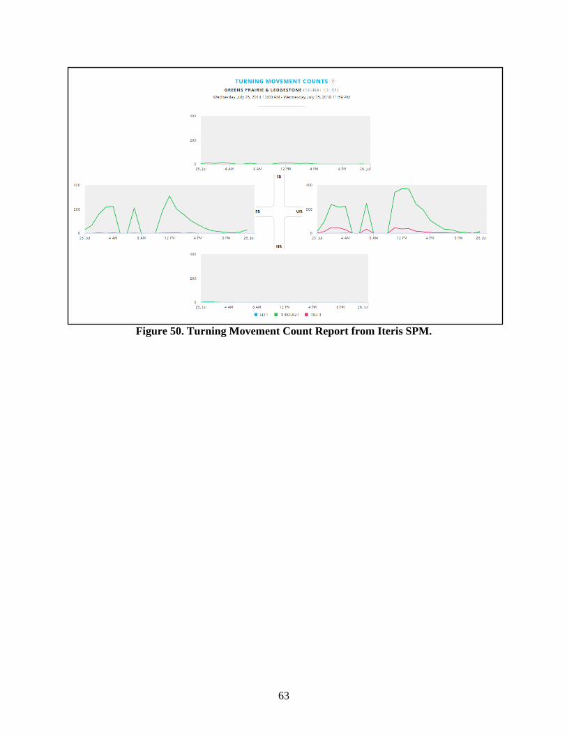
63

Figure 50. Turning Movement Count Report from Iteris SPM.

65

CHAPTER 8. GUIDELINES

Signal timing technicians and traffic engineers require a good understanding of

intersection characteristics for determining the signal controller setting. Factors including

detector length and speed limit at an approach are important for determining the signal controller

settings at intersections with an actuated signal controller. The handbook provides guidelines for

choosing the signal timing setting under different conditions. The following section discusses the

implications of results from this study on the guidelines for passage time and left turn signal

operations.

SLOW-SPEED APPROACH

Passage Time

Chapter 2 of the handbook provides the passage time for induction loops at slow-speed

approaches for various detector lengths and 85th percentile speed. Table 14 shows the

recommended passage times from the handbook. These passage time values meet the following

criteria:

• Ensure queue clearance—Prevent frequent premature gap outs and residual queues.

• Satisfy driver expectancy—Ensure the green time length is reasonable. Longer green time

might encourage conflicting street vehicles to get impatient and disrespect the signal

indication.

• Reduce max-out frequency—A high maximum allowable headway (MAH) can lead to

frequency max-out even at low volumes. This can cause large unwarranted delays on

conflicting phases.

Table 14. Passage Times for Stop Line Presence Detection (1).

66

These values were obtained using the following analytical model:

PT = MAH − Lv + Ld1.47 va

where,

• PT = passage time, seconds.

• MAH = maximum allowable headway, seconds.

• Ld = length of detection zone, ft.

• Lv = detected length of vehicle (use 17 ft).

• va = average approach speed (= 0.88* v85), mph.

• v85 = 85th percentile approach speed, mph.

According to the above results, the passage time for an approach with a 40 mph speed

limit and 60-ft and a 90-ft induction loop would be 1.5 seconds and 0.9 seconds, respectively.

Based on the results from this study, a passage time between 1 and 2 seconds is optimal for 60-ft

and 90-ft detectors. The following conclusions can be drawn from the above observation:

• Performance measures at an approach are insensitive to minor changes in detector length.

Thus, same passage times can be used for video, radar, magnetometer, and induction loop

detectors with equal detector lengths.

• This study found similar passage times as suggested in chapter 2 of traffic signal

operation handbook (9), which used an analytical model for recommending passage

times.

Detector Switching

Detector switching can be used at left turn approaches with higher volumes. It will reduce

the average delay and queue for the left turning vehicles.

HIGH-SPEED APPROACH

This study compared the scenarios when the advanced and stop bar detectors were on

separate and same channels (i.e., Option 1 and Option 3 specified in appendix C of the

handbook). Also, researchers evaluated radar detectors at high-speed approaches. Following are

the salient points based on this study:

67

• 0.5-second passage time for upstream detector provides the best performance for Radar 1,

which continuously tracks vehicles.

• Radar 2 with 1.8-second passage time for upstream detectors provides similar

performance as Radar 1.

• Advanced and stop bar detectors should be operated on separate channels when using

induction loop detectors and a passage time of 1.1 seconds for upstream detectors is

recommended.

• Non-simultaneous gap out results in fewer max-outs and are preferable when max-outs

are an issue.

• Flashing yellow arrow needs to be used on major street for permissive left turns when

using non-simultaneous gap-out setting to prevent left turning vehicle from getting

caught in yellow trap.

• Operators should also pay attention to how the particular controller handles detector

failures. To ensure that movements are not skipped when detectors fail, the operator

should verify that detectors fail in a constant call.

69

REFERENCES

1 Bonneson, J. A., Sunkari, S. R., and Pratt, M. P. (2009). Traffic signal operations handbook. Texas Transportation Institute, Texas A&M University System.

2 Middleton, D. R., Songchitruksa, P., Pratt, M. P., Sunkari, S. R., Geedipally, S. R., and Charara, H. A. (2015). Investigation of New Vehicle Detectors for High-speed Signalized Intersections. Texas Transportation Institute, Texas A&M University System.

3 Sun, D., Dodoo, L., Rubio, A., Penumala, H. K., Pratt, M., Sunkari, S., and Texas, A. (2012). Synthesis study of Texas signal control systems: technical report. Texas. Dept. of Transportation. Research and Technology Implementation Office.

4 Zimmerman, K., Bonneson, J., Pratt, M. P., and Sunkari, S. (2007). Technical Memorandum No. 2: Summary of Signal Timing Interviews with District Traffic Personnel (TxDOT Project No. 0–5629). College Station, Texas: Texas Transportation Institute, the Texas A&M University System.

5 GRIDSMART. (2018). GRIDSMART System. Retrieved June 12, 2018, from https://gridsmart.com/products/gridsmart-solution/.

6 Trafficware. (2017). Valence Pod System. Retrieved June 12, 2018, from http://www.trafficware.com/uploads/2/2/2/5/22256874/pod_system_brochure.pdf.

7 Wavetronix, LLC. (2016). SmartSensor Advance. Retrieved October 31, 2016, from http://www.wavetronix.com/en/products/smartsensor/advance/features.

8 Wavetronix, LLC. (2018). SmartSensor Matrix - Traffic Detection Devices - WavetronixTM - Product Catalog - Advanced Traffic Products, Inc. Retrieved June 12, 2018, from http://www.advancedtraffic.com/products/wavetronix/smartsensor-matrix.

9 Iteris. (2018). Vantage Vector Hybrid | Iteris, Inc. Retrieved June 12, 2018, from https://www.iteris.com/products/detection-sensors/vantage-vector-hybrid.

10 . Econolite, ASC/3 Advanced System Controllers Programming Manual, Page 11-9. Version 2.51.00, 28 February, 2012.

11 Koonce, P. (2008). Traffic signal timing manual. United States. Federal Highway Administration.

12 Chaudhary, N.A., Charara, H.A., and Sunkari, S.R. (2014). Development of NTCIP-Based Portable Traffic Signal Evaluation System. Texas Transportation Institute, Texas A&M University System.

impact of traffic signal controller settings on the use of

Documents