impact of the dense water flow over the sloping bottom on

1

Impact of the dense water flow over the sloping bottom on the open-sea

circulation: Laboratory experiments and the Ionian Sea

(Mediterranean) example

Miroslav Gačić1, Laura Ursella1, Vedrana Kovačević*1, Milena Menna1, Vlado Malačič2, Manuel Bensi1,

Maria-Eletta Negretti3, Vanessa Cardin1, Mirko Orlić4, Joël Sommeria3, Ricardo Viana Barreto5, Samuel 5

Viboud3, Thomas Valran3, Boris Petelin2, Giuseppe Siena1, Angelo Rubino5

1 National Institute of Oceanography and Applied Geophysics - OGS, Borgo Grotta Gigante 42/C, Sgonico (TS), 34010, Italy

2 National Institute of Biology, Marine Biology Station, Fornače 41, Piran, 6330, Slovenia

3 LEGI, CNRS UMR5519, University of Grenoble Alpes, Grenoble, 1209-1211 rue de la piscine, Domaine Universitaire, Saint

Martin d’Hères, 38400, France 10

4 Andrija Mohorovičić Geophysical Institute, Faculty of Science, University of Zagreb, Horvatovac 95, Zagreb, 10000, Croatia

5 University Ca’ Foscari of Venice, Dept. of Environmental Sciences, Informatics and Statistics, Via Torino 155, Mestre, 30172,

Italy

Correspondence to: Vedrana Kovačević ([email protected]) 15

Abstract. The North Ionian Gyre (NIG) displays prominent inversions on decadal scales. We investigate the role of internal

forcing, induced by changes of the horizontal pressure gradient due to the varying density of the Adriatic Deep Water (AdDW),

that spreads into the deep layers of the Northern Ionian Sea. In turn, the AdDW density fluctuates according to the circulation of

the NIG through a feedback mechanism named Bimodal Oscillating System. We set up laboratory experiments with a two-layer

ambient fluid in a circular rotating tank, where densities of 1000/1015 kg m-3 characterise the upper/lower layer, respectively. From 20

the potential vorticity evolution during the dense water outflow from a marginal sea, we analyse the response of the open-sea

circulation to the along-slope dense water flow. In addition, we show some features of the cyclonic/anticyclonic eddies that form

in the upper layer over the slope area. We illustrate the outcome of the experiments of varying density and varying discharge rates

associated with the dense water injection. When the density is high, 1020 kg m-3, and the discharge is large, the kinetic energy of

the mean flow is stronger than the eddy kinetic energy. On the other hand, when the density is smaller, 1010 kg m -3, and the 25

discharge is reduced, vortices are more energetic than the mean flow, that is, the eddy kinetic energy is larger than the kinetic

energy of the mean flow. In general, over the slope, following the onset of the dense water injection, the cyclonic vorticity

associated with a current shear develops in the upper layer. The vorticity behaves in a two-layer fashion, thus becoming anticyclonic

in the lower layer of the slope area. Concurrently, over the deep flat-bottom portion of the basin, a large-scale anticyclonic gyre

forms in the upper layer extending partly toward a sloping rim. Density record shows the rise of the pycnocline due to the dense 30

water sinking toward the flat-bottom portion of the tank. We show that the rate of increase of the anticyclonic potential vorticity is

proportional to the rate of the rise of the interface, namely, to the rate of decrease of the upper layer thickness (i.e., the upper layer

squeezing). The comparison of laboratory experiments with the Ionian Sea is made for a situation when the sudden switch from

https://doi.org/10.5194/os-2020-122Preprint. Discussion started: 8 January 2021c© Author(s) 2021. CC BY 4.0 License.

2

the cyclonic to the anticyclonic basin-wide circulation took place following the extremely dense Adriatic water overflow after the

harsh winter in 2012. We show how similar are the temporal evolution and the vertical structure in both laboratory and oceanic 35

conditions. The demonstrated similarity further supports the assertion that the wind-stress curl over the Ionian Sea is not of

paramount importance in generating basin-wide circulation inversions, as compared to the internal forcing.

1. Introduction

The effect of dense water outflow from marginal seas on the ocean circulation has attracted great attention because it represents

an important component of the global thermohaline circulation (Jungclaus and Backhaus, 1994; Dickson, 1995). Numerical and 40

laboratory studies of this phenomenon have been inspired primarily by the observations of mesoscale eddies over the dense water

outflow in the ocean (e.g., Denmark Strait, Gibraltar Strait) (Mory et al., 1987, Whitehead et al., 1990; Lane-Serff and Baines,

1998; Lane-Serff and Baines, 2000; Etling et al., 2000). The coupling between the upper layer circulation and the dense water

plume was also addressed by numerical modelling (see i.e., Spall and Price, 1998) which confirmed the formation of eddies in the

upper layer. The eddies were predicted to travel along isobaths with a characteristic speed which depends on reduced gravity, 45

bottom slope, and Coriolis parameter (Nof, 1983). The early hypotheses stated that the cyclones form by the stretching of the high

potential vorticity water column (Spall and Price, 1998). In addition to the formation of cyclonic eddies in the lighter upper part of

the water column, according to Lane-Serff and Baines (2000) secondary anticyclonic motion occupying a major part of the tank

develops. This is the only mention in the literature of this type of consequence of the dense water cascading off the slope.

The Ionian Sea, the deepest basin of the Mediterranean (maximum depth over 5000 m) together with its two adjacent basins, 50

the Adriatic and Aegean Seas, represents a key area for both the Eastern and Western Mediterranean. It is crossed by the main

Mediterranean water masses (Levantine Intermediate Water – LIW, Atlantic Water – AW) and it comprises the site of the Eastern

Mediterranean Deep Water (EMDW) formation, a process which takes place mainly in the Adriatic Sea. Adriatic Dense Water

(AdDW) overflows the Otranto Sill, represents the main component of the EMDW and spreads along the western continental slope

as a bottom-arrested current affecting the northern Ionian circulation. Only occasionally very dense water forms in the Aegean Sea 55

as it happened in the early 1990’s during the Eastern Mediterranean Transient - EMT (Roether et al., 1996; Klein et al., 1999). It

was shown that the Aegean dense water overflow affected the upper layer circulation increasing the cyclonic vorticity at the

continental slope area (Menna et al., 2019).

Analysis of long-term altimetric data reveals that the sea surface circulation in the Ionian shows peculiar characteristics

(Vigo et al., 2005): at decadal time scales it switches from a cyclonic basin-wide gyre occupying the entire northern area, to an 60

anticyclonic meandering. This fact contributes to determine the thermohaline properties of the interior Ionian basin, of the Adriatic

Sea, and of the Levantine and even the Western Mediterranean basins (Gačić et al., 2013). During the cyclonic circulation mode,

Ionian and Adriatic Seas are invaded by a highly saline Levantine water. On the other hand, during the anticyclonic circulation the

two basins are affected by the low-salinity waters of Atlantic and Western Mediterranean origin (Brandt et al., 1999). For more

than ten years the decadal inversions of the northern Ionian circulation have been the focus of Mediterranean scientists' attention 65

because the phenomenon is very prominent and involves a large part of the water column (about 2000 m deep). There has been a

long discussion about the mechanism generating such inversions and some scientists suggested, mainly based on the numerical

modelling studies, that the phenomenon is linked to the wind stress curl (see e.g., Pinardi et al., 2015; Nagy et al., 2019). Other

studies, however, showed that the wind curl variations are not strong enough to generate such changes; these studies sustain that


3

the inversions are due to the interplay between the dense water flow (Adriatic or Aegean origin) and the Ionian horizontal 70

circulation (e.g., Gačić et al. 2010; 2011; 2013; Theocharis et al., 2014; Velaoras et al., 2014). The long-term density variability

of the bottom water associated with the salinity variations in the deep-water formation site induce reversals of the horizontal

pressure gradient in the Ionian Sea and hence of the circulation pattern (Borzelli et al., 2009). The mechanism was named Adriatic-

Ionian Bimodal Oscillating System (BiOS) and described for the first time by Gačić et al. (2010). It is the purpose of this paper to

study in more detail the inversions of the open-ocean residual circulation generated by dense water flow over a sloping bottom, 75

and to understand whether this flow is strong enough to produce inversions in the upper-layer circulation like those observed in

the Ionian Sea.

To address the impact of the dense water flow on the basin-wide open-sea circulation and on the formation of anticyclonic

vorticity in the upper layer, we base our study on the analysis of the results of a series of rotating tank experiments with injection

of the dense water at the slope area. Our attention is concentrated on a two-layer system, which approximates rather well the Ionian 80

Sea conditions. Then, we examine the response of the central abyssal plain of the idealized basin to the dense water sinking and to

its along-slope flow and compare the findings with the observative studies. We also discuss mesoscale eddies and their specific

features in function of the dense water outflow rate. The dense water flow is quite often a time-limited phenomenon with the

duration of several months after the winter convection in a marginal sea; therefore, our experiments are designed to mimic this

kind of conditions. More specifically, we address the response time of the residual current field at the open sea area to the dense 85

water flow of the limited duration over the continental slope. Hence, we discuss the effect of different discharge rates of the dense

water at the slope on the surface circulation at the open sea attempting to reproduce the circulation inversions in the northern Ionian

Sea. Rubino et al. (2020), by comparing the results of experiments in the rotating tank with those obtained by a numerical model

and altimetry data, show qualitatively that the inversion of the circulation in the Ionian Sea can be solely explained in terms of the

onset of the dense water injection over the slope area. Starting from this finding, the present work goals are 1) to study the evolution 90

of potential vorticity fields both in the slope and in the central area of the rotating tank, using the outputs of three different

experiments, and 2) to compare them with vorticity obtained from altimetry (surface layer) and model derived (deep layer) flow

in the ‘real’ Ionian.

We distinguish the slope and central deep (flat bottom) areas in the tank that are equivalent to the continental slope and

deep zone of the northern Ionian basin, respectively. We compare the potential vorticity evolution in each area as related to the 95

dense water flow. The two areas are presumably controlled by different processes of the vorticity generation. In the central area

(flat bottom) the upper layer squeezing, due to the downslope sinking of the dense water to the lower layer, generates the upper

layer anticyclonic vorticity. In the slope area, the upper layer stretching due to the downslope water flow results in the generation

of the cyclonic vorticity. The lower layer on the slope is subject to squeezing and anticyclonic vorticity generation as related to the

formation of the dense water flow parallel to isobaths. 100

The linear barotropic vorticity equation for an f-plane approximation as derived from Lee-Lueng et al. (1995) in radial

coordinates for the surface layer without wind-stress forcing is:

𝛿𝜉

𝛿𝑡+

𝑓

𝐻−ℎ(𝑣 ∗ 𝑠 +

𝛿ℎ

𝛿𝑡) = 0 (1)

where ξ is the surface layer relative vorticity, f is the planetary vorticity, h and H are the lower layer and total fluid depth,

respectively, s is the bottom slope. Radial velocity component v is defined negative if directed toward the centre of the tank. In the 105

central deep area, the second term of Eq. (1) is zero (the bottom is flat). In this study we explore to what extent the linear vorticity


4

equation represents a good approximation of the flow in the slope and in the central flat-bottom areas. We discuss mechanisms

which should be taken into consideration in the case this equation does not describe satisfactorily the flow.

The paper is organized as follows: in section 2 we present experimental setup, an overview of the selected experiments and

data analysis methods. In section 3 measurements and results are described, while section 4 is dedicated to the comparison of the 110

laboratory results and Ionian Sea example. Finally, section 5 presents a summary and conclusions of the paper.

Figure 1: Scheme of the rotating tank (not in scale) and density configuration for the three experiments discussed in the paper, EXP 24,

EXP 26 and EXP 27. Left hand side: cross section with a central deep area, a slope and injectors IS1 and IS2; blue/cyan patches refer to 115 the lower/upper layers; numbers from 1 to 12 indicate inclined laser sheet levels. Right hand side: initial density in the lower/upper layers

(blue/cyan lines); density and discharge rate of the injected water (red/black colour from IS1/IS2); the thickness of the red and black

lines corresponds to discharge rates during various phases (for details see Tables 1 and 2). Only EXP 27 has both injectors active.


5

2. Data and methods 120

2.1 Experimental design

Apparatus, experimental set-up, and the velocity measurement methods at 12 levels within the tank, their horizontal resolution, as

well as the conductivity measurements (indicators of the water density) are described in detail by Rubino et al., 2020. Here we

report some essential information only.

Experiments were conducted at the Coriolis rotating platform at LEGI (Laboratoire des Écoulements Géophysiques et 125

Industriels), Grenoble, France. A circular tank of 13 m diameter and 1 m depth was adapted to simulate the sloping and deep flat-

bottom ocean geometry (Fig. 1).

The slope area was realized using an axisymmetric conical-shaped boundary descending toward the centre of the tank with a

constant slope which was determined by keeping dynamical similarity between the phenomenon to be simulated in the rotating

tank and that occurring in the Ionian Sea. The similarity results from the ratio between the gravitational (g’s) and Coriolis 130

accelerations (fu) being of the same order of magnitude for the two basins. Here g’ = gΔρ/ρ is the reduced gravity, Δρ is the density

difference between the injected water and the ambient water densities, f is the Coriolis parameter and u is the velocity component

tangential to isobaths. We introduce typical values for g’, f and u for the Ionian Sea (g’ = 1.5 x 10-3 m s-2, f = 10-4 s-1, u = 10-2 m s-

1) and take the value 5 x 10-2 for the western Ionian continental slope from the literature (Ceramicola et al., 2014). To get the

similarity between the laboratory experiments and the Ionian Sea we set the slope s in the tank to 0.1, g’ to 0.1 m s-2; for f we take 135

0.1 s-1, corresponding to one rotation day (1 revolution) lasting 120 s, while for a typical speed we chose 10-2 m s-1. In this way the

rotating tank slope angle is equal to 5.7 0 and the ratios of the two acceleration terms are of the same order of magnitude for both

basins. Hence, the slope area, with a total width of 4 m, gradually descends from the tank edge, where its height is 40 cm, down to

the tank bottom. The central deep area with constant depth has a diameter of 5 m.

140

Table 1. Initial conditions of the two layers and experiment duration: density (ρupper and ρlower) and thickness (hupper and hlower).

Note: one revolution takes 120 s, i. e., one rotation day.

ρupper

[kg/m3]

ρlower

[kg/m3]

hupper = H-h

[m]

hlower = h

[m]

duration

[rotation day]

EXP 24 999.2 1014.5 0.411 0.162 121.0

EXP 26 999.5 1013.5 0.351 0.221 126.5

EXP 27 999.5 1014.7 0.360 0.209 138.5

In this paper we consider three experiments where the ambient fluid was a two-layer system (see Tables 1 and 2, and Fig.

1 for their characteristics). The upper layer was always freshwater while the lower layer had a density of 1015 kg m-3. Dense water 145

was injected from a single injector (IS1) or from the pair of injectors (IS1 and IS2). The latter case simulated the EMT event when

presumably two dense water sources (Adriatic and Aegean Seas) were active. In the first part of all experiments (phase I, until the

45th day) the water of intermediate density (1010 kg m-3) was injected and then, to mimic the dense-water discharge event, water

of high-density (1020 kg m-3) was injected for another 45 days (phase II). Finally, experiments ended with about a 30-day interval

of the intermediate density water injection (phase III). The discharge rate was varied with the aim to study its influence on the 150

pattern of both open-sea and continental slope residual circulations, on the vorticity field and on the eddy formation.


6

Table 2. Configuration of injection sources IS1/IS2: ρ1/ρ2 and Q1/Q2 are densities and discharge rates, respectively, of injected

water.

IS1 IS2

ρ1

[kg/m3]

Q1

[10-3 m3/s]

ρ2

[kg/m3]

Q2

[10-3 m3/s]

duration/phase

[rotation days]

EXP 24 1010.2 0.8 0-45 (phase I)

1020.4 0.8 45-90 (phase II)

1010.2 0.8 90-121 (phase III)

EXP 26 1010.4 0.4 0-45 (phase I)

1019.4 0.4 45-90 (phase II)

1010.4 0.4 90-126.5 (phase III)

EXP 27 - - 1010.4 0.4 0-45 (phase I)

1019.8 1.6 1010.4 0.4 45-90 (phase II)

- - 1010.4 0.8 90-138.5 (phase III)

2.2 Data analysis 155

From the eastward and northward current components, we calculated radial and tangential velocities (in the right-hand side

coordinate system); a radial one (v) is defined positive toward the tank edge.

The horizontal spatial resolution, for all velocity components, as well as for other derived fields, like vorticity, at each of

the 12 vertical levels, is 5 x 5 cm.

For each vertical profile of density measured in the central deep area (by means of a probe Cp3, Fig. 1), we calculated the 160

Mixed Layer Depth (MLD) using the threshold method with a finite difference criterion (de Boyer Montegut et al., 2004),

considering a 1.5 kg/m3 vertical density gradient threshold and, as density reference, the value at 5 cm depth. On the other hand,

we determined the base of the pycnocline using the same method but taking as density reference, the value at 56, 50, 50 cm depth

for EXP 24, EXP 26 and EXP 27, respectively.

For what concerns the terms of the quasi-geostrophic linear vorticity equation (Eq. 1), the surface is defined as the mean of 165

levels 2 to 5, and the bottom as the mean of levels 10 and 11. Level 1 is discarded because in the central deep area it is too close

to the free surface and is therefore noisy. In the computation of the derivative of the curl, both the vorticity time series and its

derivative are smoothed with moving average on 7 points.

In the calculation of the time-lag cross correlation of vorticity over the tank slope area, we averaged vorticity values over

the levels 1 to 4 in each of three arbitrarily chosen zones. In the slope area, the levels 1-4 are well inside the upper layer of the 170

tank. The time-series are lag-shifted for a maximum positive and negative time-lags imposed by the integral time scale, i.e. the

sum of the normalized autocorrelation function, which gives the measure of the dominant correlation time scale (Emery and

Thomson, 2001), and is calculated for the entire slope area of the tank.

Mean Kinetic Energy (MKE) and Eddy Kinetic Energy (EKE) have been computed over the slope following Poulain et al.

(2001), in the surface layer defined as a depth interval containing velocity observations on levels 1 to 4. The mean velocity 175

components (eastward and northward) were calculated at each measurement grid point and within each phase.


7

We compare the current fields in the rotating tank and in the real ocean for a particular condition when a circulation inversion

event was observed in the northern Ionian Sea. Regarding the real ocean, for the surface we use the altimetry data, while for the

deep layer conditions we make use of the hydrodynamic model of the Mediterranean Forecasting System. The latter concerns the

physical reanalysis component, originating from the Copernicus Marine Service MEDSEA_REANALYSIS_PHYS_006_004 180

dataset supplied by the Nucleus for European Modelling of the Ocean (NEMO) (Simoncelli et al., 2019). This data set includes 3D

monthly-mean and daily-mean temperature, salinity, and horizontal current components (eastward and northward) covering the

entire Mediterranean Sea (https://doi.org/10.25423/MEDSEA_REANALYSIS_PHYS_006_004). The model has a horizontal grid

resolution equal to 1/16˚ (ca. 6-7 km) and 72 unevenly spaced vertical levels.

Daily absolute geostrophic velocities (AGV) derived from altimetric (surface) and model (1000 m depth) data are used to 185

estimate the relative vorticity. The resulting geostrophic vorticity fields are spatially averaged in the northern Ionian (37°-40°N;

15°-21°E), separating the centre of the northern Ionian (bins located on depths larger than 2200 m) from the slope (bins located on

depths smaller than 2200 m). Time series of these spatially averaged parameters are normalized (dividing by the Coriolis parameter)

and filtered using a 61-day moving average.

3. Results of data analyses 190

3.1 Density in the central deep area

The dense fluid sinks from the source toward the central portion of the tank within the distance on the order of one radius of

deformation and then it turns and flows along-slope (Smith, 1975; Juncklaus and Backhaus, 1994; Lane-Serff and Baines, 1998).

Due to the sinking of the dense fluid, the interface, intended as the upper boundary of the pycnocline layer, in the central deep area

of the tank rises. The rate of the interface rise is proportional to the volume discharge rate assuming that this water is distributed 195

evenly over the entire basin:

dh/dt =𝑄

𝜋𝑅(𝑡)2, (2)

where 𝑅(𝑡) = 𝑅0 + (ℎ

𝑠) is the radius of the cylinder filled by the discharge and R0 is the radius of the interface between the upper

and lower layers at t = 0.

This estimate in our case can be compared with the experimental data, i.e., the vertical density profiling near the centre of 200

the tank, which gives us the interface depth (H-h) in one point. The two values should coincide if the dense water volume is evenly

distributed over the entire tank. The interface rise results then in the squeezing of the upper layer which is proportional to the rate

of increase of the anticyclonic vorticity of the surface layer (see Eq. 1) in the central part of the basin. On the contrary, at the slope

area in the surface layer we should expect the generation of the cyclonic vorticity associated with the downslope flow of the dense

water. This dense current takes overlying ambient fluid into deeper areas causing a stretching of the water column. Conversely, 205

the bottom layer over the slope area should be squeezed due to the dense water downslope flow.

Vertical density profiling during experiments enables us to reconstruct either the MLD or the lower layer thickness (h) as a

function of time. We consider the lower layer thickness from experimental data as the total water depth in the tank minus the depth

of the MLD (red solid line in Fig. 2). The rise of the interface associated with the dense water sinking down the slope to the lower

layer of the central deep area is clear from the Hovmöller diagram. At the beginning of the experiment halocline is very thin but 210

thickens with time due to the eddy diffusion. Lower layer thickness shows different rates of change for different experiments. It is,


8

as follows from Eq. (2), directly proportional to the discharge rate and inversely proportional to the square of the radius of the

volume of the tank occupied by the injected water.

Integrating Eq. (2) we obtain:

215

ℎ = 𝑠𝑅0 {[(1 +ℎ0

𝑠𝑅0)

3

+3𝑄𝑡

𝜋𝑠𝑅03]

1

3− 1} (3)

where the subscript 0 indicates quantities at t = 0.


9

220

Figure 2: Temporal evolution of density and the Mixed Layer Depth (MLD, thick red line) for the experiments 24 (a), 26 (b) and 27 (c).

The base of the pycnocline is denoted by the thick green line. Black solid lines indicate the rotational days 45 and 90, i.e., the start and

the end of the high-density water injection, respectively (for reference see Fig. 1 and Tables 1 and 2). Black isoline step is 2 kg m-3, starting

from 1016 kg m-3 at bottom. 225

The slowest decrease of the upper layer thickness, i.e., a MLD decrease, is evident during the experiment 26, which is

characterized by the lowest dense water discharge rate. In that case, the rise (descent) of the upper (lower) boundaries of the

pycnocline layer probably depends both on the dense water sinking and the vertical mixing, which provokes the thickening of the


10

pycnocline layer. The temporal evolution of the MLD for the other two experiments is mainly due to the dense water sinking, while

the vertical mixing and turbulent diffusion probably play a minor role. This is evident from the rise of the interface (that is, the 230

upper boundary of the pycnocline) being larger than the deepening of the lower boundary. Indeed, as already pointed out, the rise

of the interface is directly proportional to the discharge rate and inversely proportional to the area of the base of the volume

occupied by the discharged water (Eq. 2). We limit our study to cases in which the filling up of the lower layer with the dense

water is to a larger extent responsible for the interface rise, i.e., to experiments 24 and 27.

We compare the MLD temporal evolution with variations of the lower layer thickness from the theoretical relationship (Eq. 235

3). The interface rise as a function of the dense water injection rate (Fig. 3) is a good approximation of the interface depth variations

in the central deep area. In fact, the inclination of the curves is remarkably close to each other. The offset between the theoretical

curve and the experimental data is present probably because the interface is not a plane but a layer of the finite thickness due to

the vertical diffusion.

240

Figure 3: Evolution of the lower layer thickness: experimental data from the vertical profiling at Cp3 (continuous red line), linear

regression curve (dashed line) and the term obtained from Eq. 4 (see text, blue line). Left panel EXP 24 and right panel EXP 27.

3.2 Vorticity in the upper and lower layers 245

The evolution of the potential vorticity of the upper layer for the central deep area is directly proportional to the dense water

injection rate (Eq. 1). Here we assume that the interface is horizontal over the entire central deep area. Dividing Eq. (1) by f and

defining now ζ as a relative vorticity normalized by the planetary vorticity f (ζ = ξ/f), and considering Eq. (2), we obtain the quasi-

geostrophic potential vorticity equation for the flat bottom:

250

𝛿𝜁

𝛿𝑡+

1

𝐻−ℎ

𝛿ℎ

𝛿𝑡= 0, (4)

or from Eq. (2) we have:

𝛿𝜁

𝛿𝑡+

1

𝐻−ℎ

𝑄

𝜋𝑅2 = 0 (5)


11

The temporal evolution of the vorticity in the two presented experiments (Fig. 4) indeed confirms the above considerations.

In the case of the experiment 24, when the dense water discharge rate was set constant to 0.8 10-3 m3 s-1, the vorticity in the upper 255

layer of the central deep area begins to decrease immediately after the start of the experiment, becoming anticyclonic already after

20 rotational days. It continues to decrease gradually until the end of phase II. The slope of the vorticity curve does not change

appreciably despite the high-density water discharge (1020 kg m-3) during phase II. At the same time, the vorticity in the upper

layer of the slope area shows monotonous increase reaching smaller absolute values than the anticyclonic vorticity in the central

deep area. Lower layer vorticity evolution (Fig. 4 left) over the slope area shows an increase in the anticyclonic vorticity, while 260

the vorticity in the central deep area is rather small.

In the case of experiment 27 (Fig. 4 right) the evolution of the vorticity in either the upper or lower layers of the deep central

and slope areas shows similar features as for the experiment 24. Differences between the two experiments stay at the initial part of

the time-series, when the dense water (1010 kg m-3) injection rate is only 0.4 10-3 m3 s-1 for the experiment 27 while for the

experiment 24 the injection rate starts with 0.8 10-3 m3 s-1 and remains constant throughout the entire duration. In experiment 27 265

the prominent vorticity variations occur only during phase II, when the high-density water (1020 kg m-3) has much stronger

discharge rate (1.6 10-3 m3s-1). About ten days after the onset of the dense water discharge the vorticity suddenly changes becoming

anticyclonic in the surface layer of the central area and almost simultaneously the flow becomes cyclonic in the upper layer of the

slope. In the central deep area, there is no clear signal of the lower layer vorticity variations. After the cessation of the high-density

water discharge (phase III), the intermediate dense water (1010 kg m-3) continues to be released at a discharge rate of 0.8 10-3 m3 270

s-1, which yields to a decrease of the anticyclonic vorticity in the surface layer of the central deep area.

Figure 4: Evolution of the average vorticity normalized by the Coriolis parameter for the EXP24 (left) and the EXP 27 (right). Vorticity 275 curves are smoothed with moving average on 15 points. In the legends, “centre” is referred to the central area of the tank (upper or

lower layer), while “slope” to the slope area (upper or lower layer).

To summarize, at the slope area the vorticity behaves in a two-layer fashion. In the case of experiment 24 in the lower layer

it becomes anticyclonic a few days after the beginning of the experiment, while in the upper layer (Fig. 4 left) it becomes cyclonic

with about ten days phase-lag with respect to the underneath part of the water column. In the case of the experiment 27 the 280

generation of the anticyclonic vorticity takes place only after the onset of the dense water injection with a high discharge rate (1.6

10-3 m3 s-1, phase II), while in the phase I we set up very low discharge rate which did not virtually affect the vorticity field. Again,


12

the response in the upper layer lags the lower layer vorticity. The vertical structure in the central deep area for both experiments

shows the occurrence of a strong anticyclonic motion in the upper layer, while in the lower layer there is no well-defined behaviour

of the vorticity. The two-layer distribution of the vorticity at the slope area can be explained in terms of a small vertical-to-lateral 285

friction ratio, whereas the single-layer circulation occurring occasionally in the center of the tank is supported by a relatively large

vertical-to-lateral friction ratio (Orlić and Lazar, 2009). This also suggests that we cannot neglect the frictional influence especially

at the slope.

Equation (5) suggests that for the flat bottom (central deep area of the rotating tank) the rate of change of the upper-layer

normalized relative vorticity, is equivalent to the inverse residence time (Monsen et al., 2002), i.e. the ratio of the dense water 290

injection rate and the volume of the upper layer. The rate of change of ζ is at the same time proportional to the time-derivative of

the lower layer thickness (Eq. 4). Variations of the upper-layer potential vorticity (Fig. 4) confirm qualitatively the results of the

Eq. (5), i.e., the time derivative of the normalized potential vorticity is smaller for the experiment 24 than for the experiment 27.

Indeed, in the case of the former experiment, the dense water discharge rate is half of the latter one. This does not mean that the

rate of change of the potential vorticity is twice as large for experiment 27 as for experiment 24 because it depends additionally on 295

the upper layer depth and on the radius R which are different for the two experiments.

From the flow field and the MLD, we can check how successfully the quasi-geostrophic potential vorticity equation for the

flat bottom does approximate the surface flow characteristics. The rate of change of the normalized potential vorticity is negatively

correlated with the rate of change of the lower layer thickness (Fig. 5) as follows from Eq. (2). In fact, the calculated correlation

coefficients (Table 3) are negative and statistically significant at the 95% confidence level. Therefore, in the flat-bottom area the 300

quasi-geostrophic potential vorticity equation approximates rather well the upper layer vorticity evolution. In addition, it is evident

that curves of the rate of change of the potential vorticity and the upper layer depth for the experiment 24 are noisier than for the

experiment 27, which is probably due to the more prominent mesoscale activity in the former experiment than in the latter, as it

will be shown later.

In the slope area we must consider also the topographic β-term (Eq. 1). Thus, we compare the rate of the vorticity change 305

with the sum of the rate of change of the lower layer thickness and the topographic β-term for the two experiments (Fig. 6). We

calculate the average radial velocity, which is negative for the downslope flow. We take the average lower layer radial velocity

over the entire slope area since the downslope dense-water flow generates stretching of the water column in the surface layer and

cyclonic vorticity. In fact, for a major part of the experiments the topographic β-term is negative (graph not shown) suggesting that

the cyclonic vorticity generation takes place due to the cross-isobath, downslope dense water flow. Generally, the correlation 310

coefficients for the slope area are smaller than for the central deep area. This confirms that at the continental slope the quasi-

geostrophic vorticity equation does not describe the vorticity variations as successfully as in the flat-bottom area. This can probably

be explained by the fact that the bottom viscous draining at the slope area is not included in the quasi-geostrophic vorticity equation.

This fact is also supported by a two-layer vorticity behaviour.

315


13

Table 3. (a) Correlation coefficients (r) between the terms of the vorticity equation (Eq. 1), for the central part of the tank. Upper

and lower limits of the coefficients are given for 95% confidence level (c.l.).

1

𝑓

𝛿𝜉

𝛿𝑡 and

1

𝐻−ℎ∗

𝛿ℎ

𝛿𝑡

Entire experiment duration Period 45-90 rot. days

r Limits 95% c.l. r Limits 95% c.l.

EXP24 -0.5466 -0.66/ -0.41 -0.6306 -0.77/-0.43

EXP27 -0.6357 -0.72/-0.53 -0.4581 -0.66/-0.20

320

Table 3. (b) Correlation coefficients (r) between the terms of the vorticity equation (Eq. 1), for the slope of the tank. Upper and

lower limits of the coefficients are given for 95% confidence level (c.l.).

1

𝑓

𝛿𝜉

𝛿𝑡 and

1

𝐻−ℎ(

𝛿ℎ

𝛿𝑡 + 𝑣 ∗ 𝑠)

Entire experiment duration Period 45-90 rot. days

r Limits 95% c.l. r Limits 95% c.l.

EXP24 0.4202 0.27/ 0.55 0.6268 0.42/ 0.77

EXP27 0.3930 0.24/ 0.52 0.4552 0.20/ 0.65

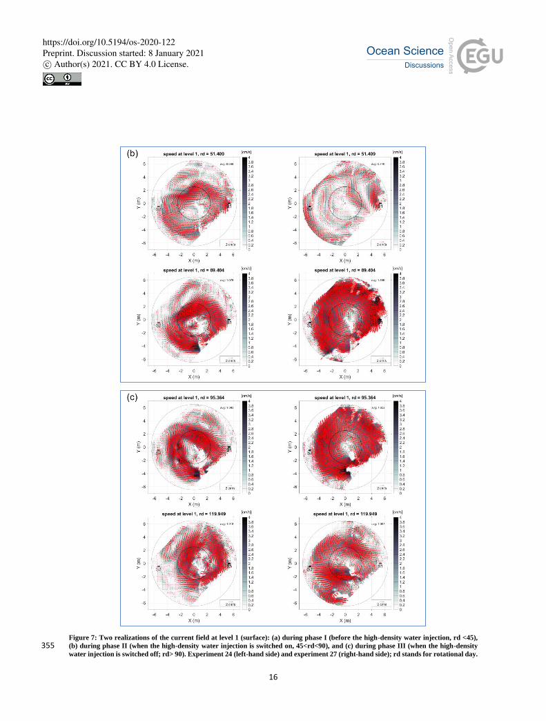
3.3 Eddies over the slope area

The time evolution of the flow field reveals that the two chosen experiments do exhibit the eddy formation on the slope but not of 325

the same intensity. Animated maps of the horizontal flow at level 1 for the entire experiment duration (animations S1 and S2 in

the Supplementary Material) support this difference. Here we illustrate the eddy formation by showing the two selected snapshots

from each of the three phases of the experiments (Fig. 7). Although eddies are not of our primary interest, we will shortly address

their characteristics for experiments 24 and 27 since, as stressed by Whitehead at al. (1990), “Isolated eddies are some of the most

beautiful structures in fluid mechanics”. Qualitatively speaking, experiment 24 shows stronger eddy activity than the experiment 330

27. To explain differences between the two experiments in terms of the eddy formation, we calculated the relative vortex stretching

and the relative importance of the viscous draining following the approach by Lane-Serff and Baines (2000). With a reference to

Fig. 3 in that paper, our calculations show indeed that the experiment 24 during the phase I falls within the parameter space where

the relationship between the relative stretching and the relative importance of the viscous draining supports the formation of eddies.


14

335

Figure 5: Time series in the central deep area of the rotating tank (flat bottom): the vorticity rate of change (

𝟏

𝒇

𝜹𝝃

𝜹𝒕, red line) and the rate

of change of the lower layer thickness (𝟏

𝑯−𝒉

𝜹𝒉

𝜹𝒕, black line) for the EXP24 (upper panel) and the EXP 27 (lower panel). For reference, see

Eq. 1, when slope s = 0.

340

Figure 6: Time series in the slope area: the vorticity rate of change (

𝟏

𝒇

𝜹𝝃

𝜹𝒕, red line) and the sum of the rate of change of the lower layer

thickness and the topographic β-term (𝟏

𝑯−𝒉(

𝜹𝒉

𝜹𝒕 + 𝒗𝒓𝒔), black line) for the EXP 24 (upper panel) and for the EXP 27 (lower panel). For

reference, see Eq. 1, when slope s = 0.1.


15

The experiment 27, on the other hand, having a discharge rate of only 0.4 10-3 m3s-1 during the phase I, falls within the overlapping 345

region and thus eddies are less likely to occur. In addition, both experiments 24 and 27 during phase II fall in the overlapping

region where the eddy formation is less likely to take place. In the final part of the experiments when the discharge rate is 0.8 10-3

m3s-1, the two experiments fall within the eddy region in the parameter space. Hence, the mesoscale eddies are likely to be formed

most of the time in the experiment 24, but only during the last part in the experiment 27.

350


16

Figure 7: Two realizations of the current field at level 1 (surface): (a) during phase I (before the high-density water injection, rd <45),

(b) during phase II (when the high-density water injection is switched on, 45<rd<90), and (c) during phase III (when the high-density 355 water injection is switched off; rd> 90). Experiment 24 (left-hand side) and experiment 27 (right-hand side); rd stands for rotational day.


17

The ratio between the eddy kinetic energy per unit mass (EKE) and the kinetic energy of the mean flow per unit mass

(MKE) measures the relative importance of eddies with respect to the mean flow. Thus, we calculate the average EKE and MKE

for both experiments for the three phases over the entire slope area, as well as the ratio between the two (Fig. 8). It is evident that

in the phase I for the experiment 24 EKE > MKE, i.e., eddies are more energetic than the mean flow (MKE), as already pointed 360

out from the relationship between the relative stretching and the relative importance of the viscous draining. For both experiments

MKE is larger than EKE in the phase II, as it also follows from the fact that the two experiments fall within the overlapping region

where eddies are less likely to be formed. Finally, in the phase III both experiments have MKE larger than EKE, although they fall

within the eddy region. This can be due to the rather high remaining energy of the mean flow from the phase II being larger than

the energy of the newly formed eddies. 365

Figure 8: Eddy kinetic energy (EKE) and kinetic energy of the mean motion (MKE) in the surface layer (mean velocities from levels 1-

4), spatially averaged over the slope area during phases I, II, and III (i.e., before, during, and after the high-density water injection) for

experiments 24 and 27.

The horizontal distribution of current vectors in the phase I shows dissimilarities between experiments 24 and 27. The 370

differences are partly due to the different dense water discharge rates (0.4 10-3 m3 s-1 for 27 and 0.8 10-3 m3 s-1 for 24). In both

experiments, we see the formation of mesoscale eddies and their progression downstream from the source. However, in the case

of the experiment 27 eddies are anticyclonic and weaker than in the case of the experiment 24. Downstream of the source of the

dense water during the experiment 24 cyclonic eddies prevail. This could be associated with the larger distance between the dense

water source and the interface in experiment 24 resulting in the longer sinking path of the dense water and the more intense 375

stretching of the water column. It should be specified that the dense water entering the upper layer during the phase I has density


18

of 2010 kg m-3 for both experiments, while the lower layer water density is 2015 kg m-3 and thus the inflowing water spreads on

the interface. The prevalence of the anticyclonic eddies during the experiment 27 is probably because the dense water source is

rather close to the interface and thus there is a weak column stretching. The anticyclonic eddy formation is due to the upper layer

squeezing because of the dense water along-slope flow on the interface. 380

During the phase II, when the dense water discharge is stronger for the experiment 27 than for the experiment 24, toward

the end of the phase the flow field shows strong clockwise basin wide circulation more spatially coherent for the experiment 27

than for the experiment 24. Eddy activity as a residual of the phase I is still prominent in the experiment 24. The phase III with the

same dense-water flow rate for both experiments shows the slowdown of the basin wide anticyclonic circulation and the relative

increase of the mesoscale activity. 385

To study in more detail the evolution of the vorticity field in the upper layer of the slope area, we calculate average vorticities

for three chosen zones at the slope of the tank (Fig. 9a) and the lagged cross-correlation between them, to estimate eddy propagation

direction and speed. As an example, we present here the results for experiment 24, which has a prominent eddy activity at the slope

area as shown earlier. The cross-correlation between zones 1 and 2 (Fig. 9b) displays a significant maximum for the positive phase-

lag at about 21 rotational days suggesting that the vorticity structures propagate prevalently anticlockwise between the two zones, 390

i.e., leaving the shallow water on their right. From this phase-lag we calculate the propagation speed which is thus about 0.3 cm s-

1 and this value is smaller than the eddy speed (1.3 cm s-1) estimated in the work by Lane-Serff and Baines (1998). On the other

hand, the cross correlation between zones 1 and 3 in general is the most significant showing the peak for a negative phase-lag at

around ten days revealing the propagation of the vorticity structures in the opposite direction, with a speed of about 1.1 cm s-1.

This is probably associated with the average advection speed of the basin-wide anticyclonic flow. The change of the propagation 395

direction can be explained by the fact that vorticity structures (eddies and meanders) firstly propagate cyclonically from the dense

water source, as noticed in various papers and experiments (see e.g., Etling et al., 2010 and references cited therein); then they start

to be advected by the basin-wide anticyclonic flow, which develops about ten days after the beginning of the experiment due to

the surface layer squeezing. The cross correlation between zones 2 and 3 is the least significant probably because zone 2 is under

the combined influence of eddies moving in opposite directions. It is evident from the horizontal distribution of current vectors 400

(see Supplementary material), that cyclonic or sometimes anticyclonic eddies continuously form downstream of the dense water

source due to the upper-layer stretching in the case of the high-density water spreading, or to the upper-layer squeezing associated

with the intermediate density (1010 kg m-3) water spreading along the interface between the upper and lower layers. These eddies

move counterclockwise until they experience the advection by the anticyclonic basin-wide flow and start moving in the opposite

direction. 405


19

Figure 9: Vorticity correlations over the slope for EXP24. Position of the three selected zones (a); time-lagged correlation coefficients

(solid line) between zones 1 and 2 (b), between zones 1 and 3 (c); between zones 2 and 3 (d). Upper and lower limits of the coefficients,

corresponding to the 95% confidence level, are indicated by dashed-dot lines. Rose shaded areas indicate positive correlation at 95%

confidence limits. The limits for the maximum time lag were set by the calculated correlation time for the entire slope area, equal to 410 about 22 rotation days.

4. Comparison between the laboratory experiment and the Ionian Sea

We compare the laboratory experiments, which simulate the effects of the dense water overflow into the real ocean with an event

occurred in the northern Ionian Sea characterized by the sudden change of the circulation as a consequence of the very dense water

flow from the Adriatic Sea following harsh winter (Mihanović et al., 2012; Bensi et al., 2013; Raicich et al., 2013; Gačić et al., 415

2014; Querin et al., 2016). This discharge event, which took place in 2012, generated an abrupt and temporary inversion of the

upper-layer Ionian circulation from cyclonic to anticyclonic. Gačić et al. (2014) were able to determine accurately the start and the

cessation of the dense water flow thanks to an ample availability of in situ data mainly from floats. They estimated that the sudden

inversion of the horizontal circulation from cyclonic to anticyclonic took place in June 2012 and subsequent return to cyclonic in

February/March 2013. To carry out the comparison with the tank experiment, we determine the response of the surface geostrophic 420

flow field to the dense water discharge event from satellite altimetry data. In addition, we use the density field during the event, as


20

well as the subsurface flow, from the hydrodynamic model. We simulate the real situation by releasing the dense water in the tank

for a limited time interval during the experiment (45 rotation days). As mentioned earlier, the flow field response in the tank was

observed from the current data while the density field variations were detected from the vertical profiling in the central deep area

of the tank. 425

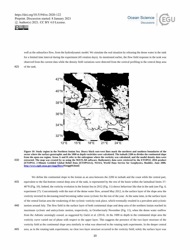
Figure 10: Study region in the Northern Ionian Sea. Heavy black east-west lines mark the northern and southern boundaries of the

sector where the surface geostrophic and the 1000 m depth vorticities were calculated. The isobath 2200 m divides the continental slope

from the open-sea region. Areas A and B refer to the subregions where the vorticity was calculated, and the model density data were

extracted. The map was created by us using the MATLAB software. Bathymetry data were retrieved by the ETOPO2_2016 product 430 (ETOPO2, 2-Minute Gridded Global Relief Data (ETOPO2v2), NOAA, World Data Service for Geophysics, Boulder, June 2006.

http://www.ngdc.noaa.gov/mgg/fliers/01mgg04.html)

We define the continental slope in the Ionian as an area between the 2200 m isobath and the coast while the central part,

equivalent to the flat-bottom central deep area of the tank, is represented by the rest of the basin within the latitudinal limits 37-435

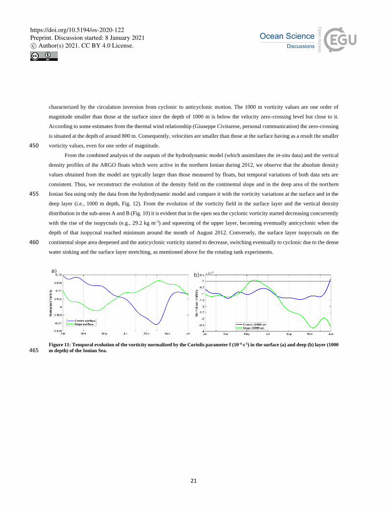
40°N (Fig. 10). Indeed, the vorticity evolution in the Ionian Sea in 2012 (Fig. 11) shows behaviour like that in the tank (see Fig. 4,

experiment 27). Concomitantly with the start of the dense water flow, around May 2012, in the surface layer of the slope area the

vorticity inverted its decreasing trend becoming rather soon cyclonic for the rest of the year. At the same time, in the surface layer

of the central Ionian area the weakening of the cyclonic vorticity took place, which eventually resulted in a prevalent anticyclonic

motion around July. The flow field in the surface layer of both continental slope and deep area of the northern Ionian reached its 440

maximum cyclonic and anticyclonic motion, respectively, in October/early November (Fig. 11), when the dense water outflow

from the Adriatic seemingly ceased, as suggested by Gačić et al. (2014). At the 1000 m depth in the continental slope area the

vorticity curve varied out of phase with respect to the upper layer. This suggests the presence of the two-layer structure of the

vorticity field at the continental slope area similarly to what was observed in the rotating tank experiments. In the deeper central

area, as in the rotating tank experiments, no clear two-layer structure occurred in the vorticity field; solely the surface layer was 445


21

characterized by the circulation inversion from cyclonic to anticyclonic motion. The 1000 m vorticity values are one order of

magnitude smaller than those at the surface since the depth of 1000 m is below the velocity zero-crossing level but close to it.

According to some estimates from the thermal wind relationship (Giuseppe Civitarese, personal communication) the zero-crossing

is situated at the depth of around 800 m. Consequently, velocities are smaller than those at the surface having as a result the smaller

vorticity values, even for one order of magnitude. 450

From the combined analysis of the outputs of the hydrodynamic model (which assimilates the in-situ data) and the vertical

density profiles of the ARGO floats which were active in the northern Ionian during 2012, we observe that the absolute density

values obtained from the model are typically larger than those measured by floats, but temporal variations of both data sets are

consistent. Thus, we reconstruct the evolution of the density field on the continental slope and in the deep area of the northern

Ionian Sea using only the data from the hydrodynamic model and compare it with the vorticity variations at the surface and in the 455

deep layer (i.e., 1000 m depth, Fig. 12). From the evolution of the vorticity field in the surface layer and the vertical density

distribution in the sub-areas A and B (Fig. 10) it is evident that in the open sea the cyclonic vorticity started decreasing concurrently

with the rise of the isopycnals (e.g., 29.2 kg m-3) and squeezing of the upper layer, becoming eventually anticyclonic when the

depth of that isopycnal reached minimum around the month of August 2012. Conversely, the surface layer isopycnals on the

continental slope area deepened and the anticyclonic vorticity started to decrease, switching eventually to cyclonic due to the dense 460

water sinking and the surface layer stretching, as mentioned above for the rotating tank experiments.

Figure 11: Temporal evolution of the vorticity normalized by the Coriolis parameter f (10-4 s-1) in the surface (a) and deep (b) layer (1000

m depth) of the Ionian Sea. 465


22

Figure 12: Vorticity variations (upper panels) as in Fig. 11 and the Hovmöller diagram of the potential density anomaly field (lower

panels) for the continental slope - area A (left hand side) and the open-sea - area B (right hand side), based on the numerical model data,

see Fig. 10 for the position of areas A and B. Please note different scales of the surface (left) and deep (right) vorticity values. 470

Similarity between the Ionian and the rotating tank can also be quantified by comparing the respective vorticity rate of

change, i.e., 𝛿𝜁

𝛿𝑡. It is inversely proportional to the residence time of the upper layer (see Eq. 5). Hence the ratio of the inclination

of the vorticity curve for the Ionian and the rotating tank, is inversely proportional to the ratio of their residence times associated

with the dense water flow rate. Calculating the receiving volume of the Ionian Sea and the tank and knowing the dense water flow 475

rate in the tank for the experiment 27 (1.6 10-3 m3 s-1) and the dense water outflow from the Adriatic (on average 3 105 m3 s-1

according to Lascaratos, 1993), we estimate the ratio between the residence times. On the other hand, we estimate 𝛿𝜁

𝛿𝑡 from vorticity

curves both for the rotating tank and the Ionian (see Figs. 4 and 11) and the ratio of the vorticity rate of change of the two basins.

Our results indeed show that the ratio between residence times of the Ionian Sea and the rotating tank is of the same order of

magnitude as the ratio of the vorticity rate of change in the rotating tank and in the Ionian Sea. This confirms the dynamical 480

similarities of the dense water flow in the two basins.

5. Summary and conclusions

The decadal inversions of the horizontal circulation, peculiar phenomena in the Ionian Sea, according to the BiOS theory (see e.g.,

Rubino et al., 2020 and papers cited therein) are not wind-induced but are due to inversions of the internal density gradients.

Observations reveal that a reversal can occur very rapidly, i.e., even at time scales on the order of a month (see Gačić et al., 2014). 485

Here we simulate this type of situation in the rotating tank and compare it with observational data gathered in the Ionian basin

during the 2012 exceptional dense water overflow. This remarkable phenomenon occurred when, due to the harsh 2012 winter the


23

BiOS cyclonic mode which started in 2011, was suddenly interrupted and reversed to the anticyclonic flow. To carry out the

comparison between such reversal and the tank experiments, we focus on two laboratory experiments where different dense water

discharge rates created the similar dynamics to that observed in the real ocean. For the two experiments analysed in detail the 490

ambient fluid consists in two layers: the upper one is made of freshwater while the lower layer has a density of 1015 kg m-3. In the

first part of the experiments, water of 1010 kg m-3 was discharged for a period of 45 rotational days (1 day = 120 sec) after which

a high-density water of 1020 kg m-3 was released until the 90th day. We vary the dense water flow rates of the two experiments and

observe the evolution of the current field. The formation of the large basin-wide anticyclonic gyre in the surface layer of the central

flat-bottom area of the tank initiates after the dense water flow starts. Concurrently, over the slope area in the upper layer the 495

cyclonic vorticity manifests itself as a series of counter-clockwise travelling mesoscale cyclones (leaving the shallow water on

their right) or in the form of a cyclonic basin-wide shear. We show that the mesoscale eddy activity depends on the dense water

discharge rate. Also, the mesoscale eddies propagate anticlockwise from the dense water source, until the onset of the basin-wide

anticyclonic circulation. Then, the vortices are advected by the mean basin-wide flow in the opposite direction. In the lower layer

of the slope area, instead, an anticyclonic vorticity is generated and therefore in that portion of the tank the current field behaves 500

in a two-layer fashion from the point of view of the vorticity pattern. The vorticity in the Ionian Sea shows a vertical structure both

in the continental slope and in the central deep area like in the rotating tank. We show that the evolution of the flow field in the

Ionian following the dense water outflow from the Adriatic is dynamically similar to the flow field in the rotating tank following

the dense water injection. The similarity is shown for the experiment with the dense water discharge rate of 1.6 10-3 m3 s-1 when

the ratio between the vorticity rate of change in the Ionian and in the tank is of the same order of magnitude as the inverse of the 505

ratio of the residence times. This laboratory experiment confirms that the internal forcing, the only forcing applied in the rotating

tank, is sufficient to create inversions of the basin-wide cyclonic circulation to the anticyclonic one in the Ionian Sea as already

hypothesized by the BiOS theory.

Data availability 510

All used data sets can be made available by request to the first and corresponding author.

Supplement

Link to S1&S2.zip

Authors contribution

MG, AR, JS designed the laboratory experiments; MG prepared the manuscript with the help of all co-authors; AR, LU, VK, 515

VM, MEN, VC, MO, JS, MM contributed to writing and editing of the manuscript and participated in the theoretical aspect

discussions; LU, VK, MM, MB, MEN, VC, RVB carried out the data analysis using specifically designed analysis routines; VK,

MB, MEN, VC, JS, RVB, SV, BP, GS, MG, AR performed the laboratory experiments.


24

Competing interest

The authors declare that they have no known competing financial interests or personal relationships that could have appeared to 520

influence the work reported in this paper.

Acknowledgments

We greatly appreciate the technical and scientific support offered by the LEGI staff during the project implementation. We thank

G. Civitarese for his enthusiasm and important contribution to the early work in the project preparation. We are grateful to Achim 525

Wirth for making available his design of the injectors used in the experiments. Finally, our thanks go to P. Del Negro for her

encouragement and interest in our project.

Financial support

The project BiOS - CRoPEx has received funding from the European Union’s Horizon 2020 research and innovation program

under grant agreement No. 654110, HYDRALAB+. 530

References

Bensi, M., Cardin, V., Rubino, A., Notarstefano, G., and Poulain, P. M.: Effects of winter convection on the deep layer of the

Southern Adriatic Sea in 2012, J. Geophys. Res. Oceans, 118, doi:10.1002/2013JC009432, 2013.

Borzelli, G.L.E, Gačić, M., Cardin, V. and Civitarese, G.: Eastern Mediterranean Transient and reversal of the Ionian Sea

circulation. Geophys. Res. Lett., 36, L15108, doi:10.1029/2009GL039261, 2009. 535

Brandt, P., Rubino, A., Quadfasel, D., Alpers, W., Sellschopp, J. and Fiekas H. V.: Evidence for the influence of Atlantic-Ionian

Stream fluctuations on the tidally induced internal dynamics in the Strait of Messina, J. Phys. Oceanogr., 29, 1071-1080, 1999.

Cazenave, A., Cabanes, C., Dominh, K., and Mangiarotti, S.: Recent sea level change in the Mediterranean Sea revealed by

TOPEX/Poseidon satellite altimetry. Geophys. Res. Lett., 28, 1607-1610, 2001.

Ceramicola, S., Praeg, D., Coste, M., Forlin, E., Cova, A., Colizza, E., and Critelli, S.: Submarine mass-movements along the 540

slopes of the active Ionian continental margins and their consequences for marine geohazards (Mediterranean Sea). In:

Submarine Mass Movements and Their Consequences. Advances in Natural and Technological Hazards Research, 37, pp. 295-

306. DOI: 10.1007/978-3-319-00972-8_26, 2014.

Civitarese, G., Gačić, M., Eusebi Borzelli, G. L., and Lipizer, M.: On the impact of the Bimodal Oscillating System (BiOS) on the

biogeochemistry and biology of the Adriatic and Ionian Seas (eastern Mediterranean), Biogeosciences, 7, 3987–3997, 2010, 545

doi:10.5194/bg-7-3987-2010, 2010.

de Boyer Montégut, C.: Mixed layer depth over the global ocean: An examination of profile data and a profile-based climatology.

J. Geoph. Res. 109. https://doi.org/10.1029/2004JC002378, 2004.


25

Emery, W. J. and Thomson, R.E.: Data Analysis Methods in Physical Oceanography. 2nd and revised ed., 638 pp., Elsevier Science

B.V., 2001. 550

Etling, D., Gelhardt, F., Schrader, U., Brennecke, F., Kuehn, G., Chabert d’Hieres, G., and Didelle, H.: Experiments with density

currents on a sloping bottom in a rotating fluid. Dyn. Atm. Oceans, 31, 139-164, 2000.

Dickson, R. R.: The Local, Regional, and Global Significance of Exchanges through the Denmark Strait and Irminger Sea, National

Research Council. Natural Climate Variability on Decade-to-Century Time Scales. Washington, DC: The National Academies

Press. https://doi.org/10.17226/5142, 1995. 555

Gačić, M., Eusebi Borzelli, G. L., Civitarese, G., Cardin, V., and Yari, S.: Can internal processes sustain reversals of the ocean

upper circulation? The Ionian Sea example, Geoph. Res. Lett., 37, L09608, 2010, doi:10.1029/2010GL043216, 2010.

Gačić, M., Civitarese, G., Euzebi Borzelli, G. L., Kovačević, V., Poulain, P.-M., Theocharis, A., Menna, M., Catucci, A. and

Zarokanellos, N.: On the relationship between the decadal oscillations of the Northern Ionian Sea and the salinity distributions

in the Eastern Mediterranean, J. Geoph. Res., 116, C12002, doi:10.1029/2011JC007280, 2011. 560

Gačić, M., Civitarese, G. Kovačević, V., Ursella, L., Bensi, M., Menna, M., Cardin, V., Poulain, P.-M., Cosoli, S., Notarstefano

G., and Pizzi, C.: Extreme winter 2012 in the Adriatic: an example of climatic effect on the BiOS rhythm. Ocean Science, 10,

513-522, https://doi.org/10.5194/os-10-513-2014, 2014.

Gačić, M., Schroeder, K., Civitarese, G., Cosoli, S., Vetrano, A., and Eusebi Borzelli, G. L.: Salinity in the Sicily Channel

corroborates the role of the Adriatic–Ionian Bimodal Oscillating System (BiOS) in shaping the decadal variability of the 565

Mediterranean overturning circulation. Ocean Science, 9, 83–90, www.ocean-sci.net/9/83/2013/ doi:10.5194/os-9-83-2013,

2013.

Jungclaus, H. J. and Backhous, J. O.: Application of a transient reduced gravity plume model to the Denmark Strait Overflow. J.

Geoph. Res., Atmospheres, 99(C6):12,375-12,396 1994.

Klein, B., Roether, W., Manca, B., Bregant, D., Beitzel, V., Kovačević, V., and Luchetta, A.: The large deep-water transient in the 570

Eastern Mediterranean. Deep-Sea Res., Part I-Oceanographic Research Papers - Deep-Sea Res. Part I-Oceanogr. Res. 46. 371-

414. 10.1016/S0967-0637(98)00075-2, 1999.

Lane-Serff, G. F., and Baines, P. G.: Eddy formation by dense flows on slopes in a rotating fluid. J. Fluid Mech. 363, 229-252,

1999.

Lane-Serff, G. F. and Baines, P. G.: Eddy formation by overflows in stratified water. J. Phys. Oceanogr., 30, 327–337, 2000. 575

Lascaratos, A.: Estimation of deep and intermediate water mass formation rates in the Mediterranean Sea. Deep-Sea Res. II, 40,

1327-1332, 1993.

Lee-Lueng, F. and Davidson, R. A.: A note on the barotropic response of sea level to time-dependent wind forcing. J. Geophys.

Res., 100, C2, 24955-24963, 1995.

Menna, M., Reyes Suarez, N. C., Civitarese, G., Gačić, M., Poulain, P.-M., and Rubino, A.: Decadal variations of the circulation 580

in the Central Mediterranean and its interactions with mesoscale gyres. Deep-Sea Research II, 164, 1-24, 2019,

https://doi.org/10.1016/j.dsr2.2019.02.004, 2019.

Mihanović, H., Vilibić, I., Carniel, S., Tudor, M., Russo, A., Bergamasco, A., et al.: Exceptional dense water formation on the

Adriatic shelf in the winter of 2012. Ocean Science 9(6):3701-3721, DOI: 10.5194/osd-9-3701-2012, 2012.

Monsen, N. E., Cloem, J. E., Lucas, L. V., and Monismith, S. G.: A comment on the use of flushing time, residence time, and age 585

as transport time scales. Limnology and Oceanography, 1545-1553, 2002.


26

Mory, M., Stern, M. E., and Griffiths, R. W.: Coherent baroclinic eddies on a sloping bottom. J. Fluid Mech. 183, 45–62, 1987.

Nagy, H., Di Lorenzo, E., and El-Gindy, A.: The impact of climate change on circulation patterns in the Eastern Mediterrnaean

Sea upper layer using Med-ROMS model, Progress in Oceanogr., 175(C):226-244, DOI: 10.1016/j.pocean.2019.04.012, 2019.

Nof, D.: The translation of isolated cold eddies on a sloping bottom. Deep-Sea Res., 30, 171-182, 1983. 590

Orlić, M. and Lazar, M.: Cyclonic versus Anticyclonic Circulation in Lakes and Inland Seas. J. Phys. Oceanogr., 19, 9, 2247-2263,

DOI: 10.1175/2009JPO4068.1, 2009.

Pinardi, N., Zavatarelli, M., Adani, M., Coppini, G., Fratianni, C., Oddo, P., Simoncelli, S., Tonani, M., Lyubartsev, V., Dobricic,

S., and Bonaduce, A.: Mediterranean Sea large-scale low-frequency ocean variability and water mass formation rates from 1987

to 2007: A retrospective analysis, Progress in Oceanogr., 132, 318-332, 2015 595

Poulain, P.-M.: Adriatic Sea surface circulation as derived from drifter data between 1990 and 1999, J. Mar. Syst., 29, 3-32, 2001.

Querin, S., Bensi, M., Cardin, V., Solidoro, C., Bacer, S., Mariotti, L., et al.: Saw‐tooth modulation of the deep‐water thermohaline

properties in the southern Adriatic Sea. J. Geoph. Res.: Oceans, 4585–4600, 2016.

Raicich, F., Malačič, V., Celio, M., Giaiotti, D., Cantoni, C., R. Colucci, R., Čermelj, B., and Pucillo, A.: Extreme air-sea

interactions in the Gulf of Trieste (North Adriatic) during the strong Bora event in winter 2012, J. Geophys. Res. Oceans, 118, 600

5238–5250, doi:10.1002/jgrc.20398, 2013.

Roether, W., Manca, B. B., Klein, B., Bregant, D., Georgopoulos, D., Beitzel, V., Kovačević, V., and Lucchetta, A.: Recent changes

in eastern Mediterranean deep waters, Science, 271, 333 – 335, 1996

Rubino, A., Gačić, M, Bensi, M., et al.:Experimental evidence of long-term oceanic circulation reversals without wind influence

in the North Ionian Sea. Sci. Rep. 10, 1905 https://doi.org/10.1038/s41598-020-57862-6, 2020. 605

Smith, P. C.: A streamtube model for the bottom boundary currents in the ocean, Deep-Sea Research, 22, pp. 853-874, 1975.

Simoncelli, S., Fratianni, C., Pinardi, N., Grandi, A., Drudi, M., Oddo, P., and Dobricic, S.: Mediterranean Sea Physical Reanalysis

(CMEMS MED-Physics) [Data set]. Copernicus Monitoring Environment Marine Service (CMEMS).

https://doi.org/10.25423/MEDSEA_REANALYSIS_PHYS_006_004, 2019.

Spall, M. A. and Price, J. F.: Mesoscale variability in Denmark Strait: The PV outflow hypothesis. J. Phys. Oceanogr., 28, 1598-610

1623, 1998.

Vigo, I., Garcia, D., and Chao, B. F.: Change of sea level trend in the Mediterranean and Black seas, J. Mar. Res., 63, 1085−1100,

doi:10.1357/002224005775247607, 2005.

Yan, H-M., Zhong, M., and Zho, Y-Z.: Determination of degree of freedom of digital filtered time series with an application to the

correlation analysis between the length of day and the southern oscillation index, Chinese Astronomy and Astrophysics, 28, 120-615

126, doi: 10.1016/j.chinastron.2004.01.014, 2004.

Theocharis, A., Krokos, G., Velaoras, D., and Korres, G.: An internal mechanism driving the alternation of the Eastern

Mediterranean dense/deep water sources, In The Mediterranean Sea: Temporal Variability and Spatial Patterns, edited by G. L.

E. Borzelli, et al., AGU Geophys. Monogr. Ser., 202, pp. 113–137, John Wiley, Oxford, U. K., doi:10.1002/9781118847572.ch8,

2014. 620

Velaoras, D., Krokos, G., Nittis, K., and Theocharis, A.: Dense intermediate water outflow from the Cretan Sea: A salinity driven,

recurrent phenomenon, connected to thermohaline circulation changes. J. Geophys. Res. 119, 4797–4820, 2014.

Whitehead, J. A., Stern, M. E., Flierl, G. R., and Klinger, B. A.: Experimental observations of baroclinic eddies on a sloping

bottom. J. Geophys. Res., 95, 9585–9610,1990.


impact of the dense water flow over the sloping bottom on

Documents