image formation. input - digital images intensity images – encoding of light intensity range...
TRANSCRIPT

Image Formation

Input - Digital Images
Intensity Images – encoding of light intensity
Range Images – encoding of shape and distance
They are both a 2-D array or matrix of numbers
These numbers could be 8-bit (most cases), 10-bit, or 12-bit data for black and white images and 24-bit data (Red, Green, and Blue) for color images.
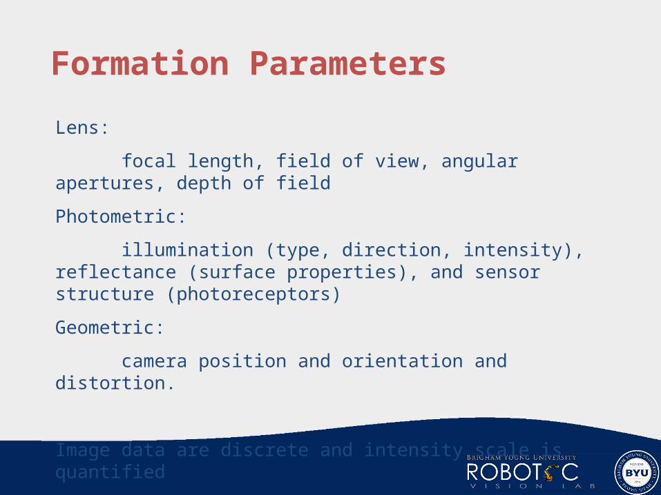
Formation Parameters
Lens:
focal length, field of view, angular apertures, depth of field
Photometric:
illumination (type, direction, intensity), reflectance (surface properties), and sensor structure (photoreceptors)
Geometric:
camera position and orientation and distortion.
Image data are discrete and intensity scale is quantified
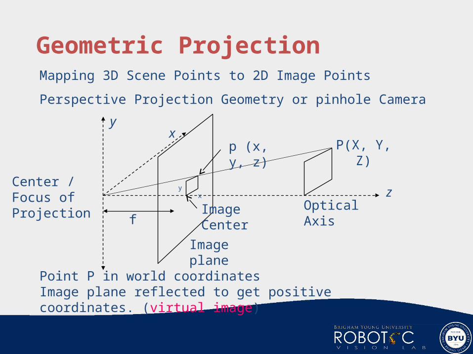
Geometric ProjectionMapping 3D Scene Points to 2D Image Points
Perspective Projection Geometry or pinhole Camera
z
f
yx
xy
P(X, Y, Z)
Image plane
Point P in world coordinatesImage plane reflected to get positive coordinates. (virtual image)
Center / Focus of Projection
Optical AxisImage Center
p (x, y, z)

Camera frame – the x, y, z coordinate system
Perspective Projection
? Transformation is not one-to-one
Recognizing or reconstructing objects in a 3D scene from one image is an ill-posed problem.
What are we trying to do?
Recapture information about the 3D original scene that an image depicts.
Z
Xfx
Z
Yfy

Full-Perspective Camera Fundamental Equations
They are nonlinear – magnification ratio (x/X) depends on Z
Weak-Perspective (or scaled orthography) Camera Fundamental Equations
They are linear – magnification ratio (x/X) is fixed
The scene depth is small relative to the average distance from the camera
Orthographic Projection is usually unrealistic
m = 1
Z
Xfx
Z
Yfy
Z
Xfx
Z
Yfy
Z
fm

Image Digitization
Sampling and Quantization:
A continuous function f(x,y) is sampled into a matrix with M rows and N columns.
The continuous range of the image function is split into K intervals.
Sampling Interval Δx, Δy
Square-pixel camera Δx = Δy otherwise
Sampling function
),(),(1 1
ykyxjxyxsM
j
N
k
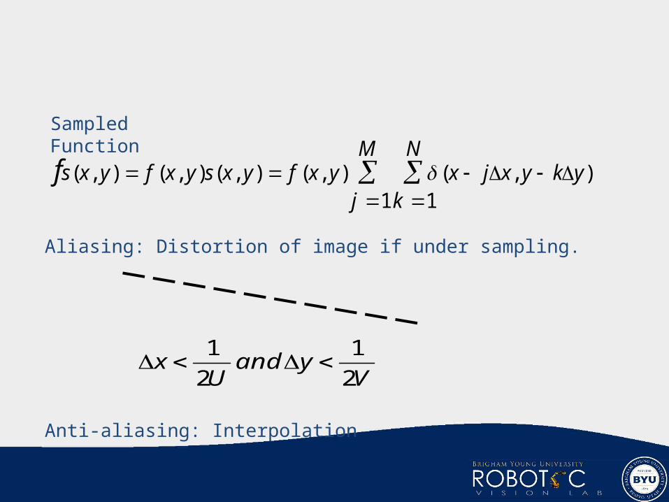
Sampled Function
M
j
N
kykyxjxyxfyxsyxfyxsf
1 1),(),(),(),(),(
Aliasing: Distortion of image if under sampling.
Vyand
Ux
2
1
2
1
Anti-aliasing: Interpolation
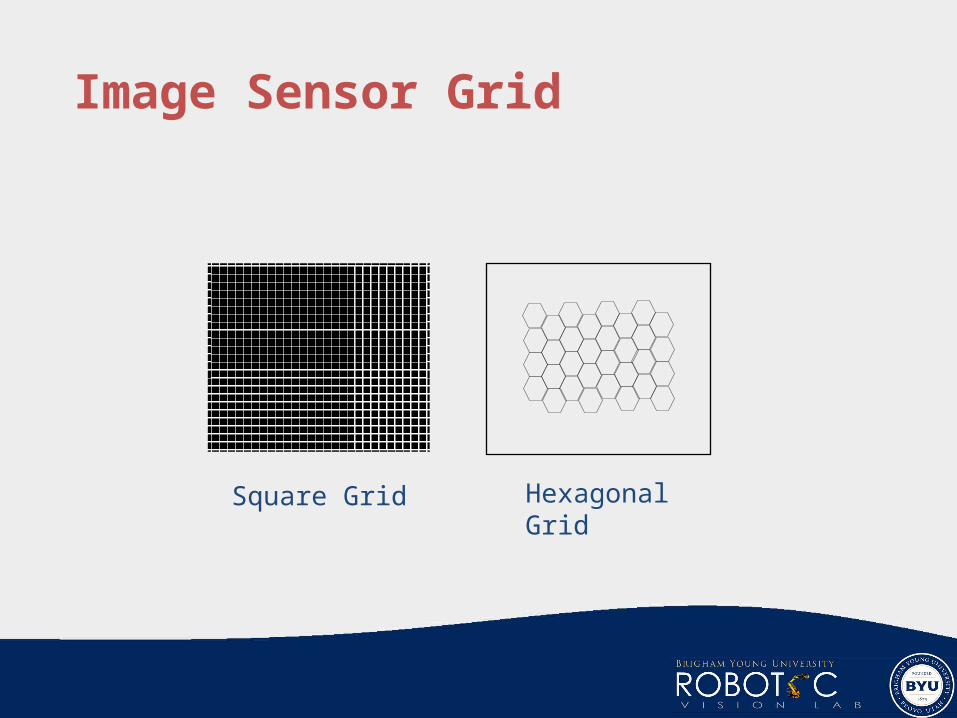
Image Sensor Grid
Square Grid Hexagonal Grid

Quantization
K intervals = 2b
b = number of bits
8 bits per pixel are commonly used.
1 bit for binary image
4 and 6 bits low resolution
10 and 12 bits high resolution
24 bits for color images

Digital Image Properties
Picture elements with finite size
Usually are arranged into a rectangular grid
2-D matrix whose elements are integer numbers
Euclidean Distance: Computationally Expensive22 )()(),(),,[( kjhikhjiDE
City Block
Chessboard
Quasi-Euclidean
|||| kjhiD
|}||max{| kjhiD

Euclidean :
City Block :
Chessboard :
Quasi-Euclidean :
2.236
3
2
2.414
BABABA yyxxppd )12(),( BABA yyxx
BABABA yyxxppd )12(),(
when
otherwise

Histogram
Contrast
local change in brightness
Image Quality
correlation, mean quadratic difference,mean absolute difference, maximum absolute difference
Image Noise
random degradation
from acquisition, transmission, processing

Problems in Digital ImagesGeometry Distortion: lens imperfection light beams are not bent correctly
Intensity Distortion: lens or light imperfectionintensity brighter in the center
Scattering: beams or radiation bent or dispersed by the medium through which they pass, aerial and satellite images (water vapor)
Blooming: imperfect insulation between cells, saturation and spill/leak to neighboring cells, very bright region
CCD Variations: imperfect manufacturing, different response to the same light
Clipping or Wrap-Around: saturation or loss high order bits loses sensitivity for bright objects, darker than it should be
Chromatic Distortion: different wavelengths bent differentlysame scene spot may show on different pixelssharp edge (step function) becomes blurry (ramp function)
Quantization Effects: mapping intensity to one of discrete gray values mixing and rounding problems, spatial quantization effects


Other Terms
Nominal Resolution: 500×500 pixels for a 10”×10” area
Sub-pixel Resolution: interpolation or other algorithms such as sub-pixel edge detection
Field of View (FOV): Angular Field of View
Depth of Field (DOF): Range of Depth in Focus
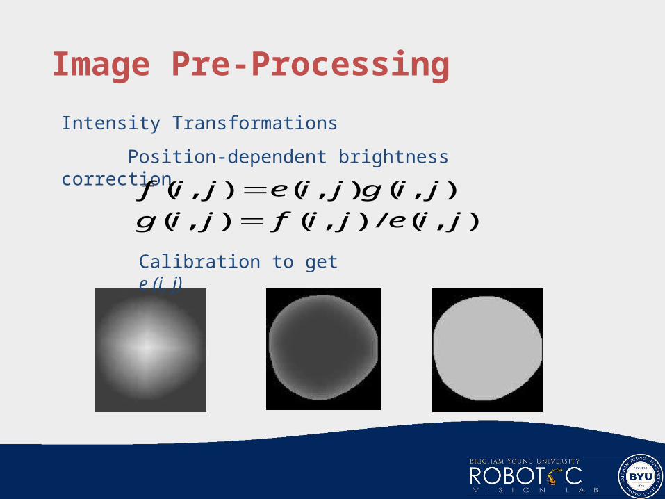
Image Pre-Processing
Intensity Transformations
Position-dependent brightness correction
),(/),(),(
),(),(),(
jiejifjig
jigjiejif
Calibration to get e (i, j)

Position-independent Brightness Correction
Look-up-table (LUT)
q = f (p)
p
q
Image Pre-Processing

Image Pre-Processing

Geometry Transformation (distortion)
Line Non-linearity Distortion
Panoramic Distortion
Skew Distortion
Distance Distortion
Perspective Distortion

Geometry Transformations
Pixel Co-ordinates Transformations
Intensity Interpolation
),(' yxTx x ),(' yxTy y
Image Pre-Processing

Image Pre-Processing
Pixel Co-ordinates Transformations
Maps the coordinates of the input image pixels to the point in the output image.
krm
r
rm
krk yxax
0 0
' krm
r
rm
krk yxby
0 0
'
It is a linear transformation. Needs pairs of (x,y) and (x’, y’) to calculate the coefficients. Usually low-order approximating polynomials m=2 or m=3 are used.
More points than coefficients are used to provide robustness for the least mean square method (SVD)

Points for calibration must be distributed to express the geometry transformation
The higher the degree of the approximating polynomial, the more sensitive to the distribution of these points.
Bilinear Transform: warping
Affine Transform: rotation, translation, scaling, skewing
xybybxbby
xyayaxaax
3210
3210
'
'
ybxbby
yaxaax
210
210
'
'
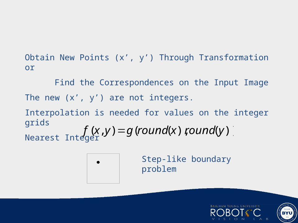
Obtain New Points (x’, y’) Through Transformation or
Find the Correspondences on the Input Image
The new (x’, y’) are not integers.
Interpolation is needed for values on the integer grids
Nearest Integer
))(),((),( yroundxroundgyxf
Step-like boundary problem

Linear Interpolation
),1()1(),()1)(1(),( klgbaklgbayxf )1,1()1,()1( klabgklgab
(x,y)
(l,k)
a
bBlurry on the edge
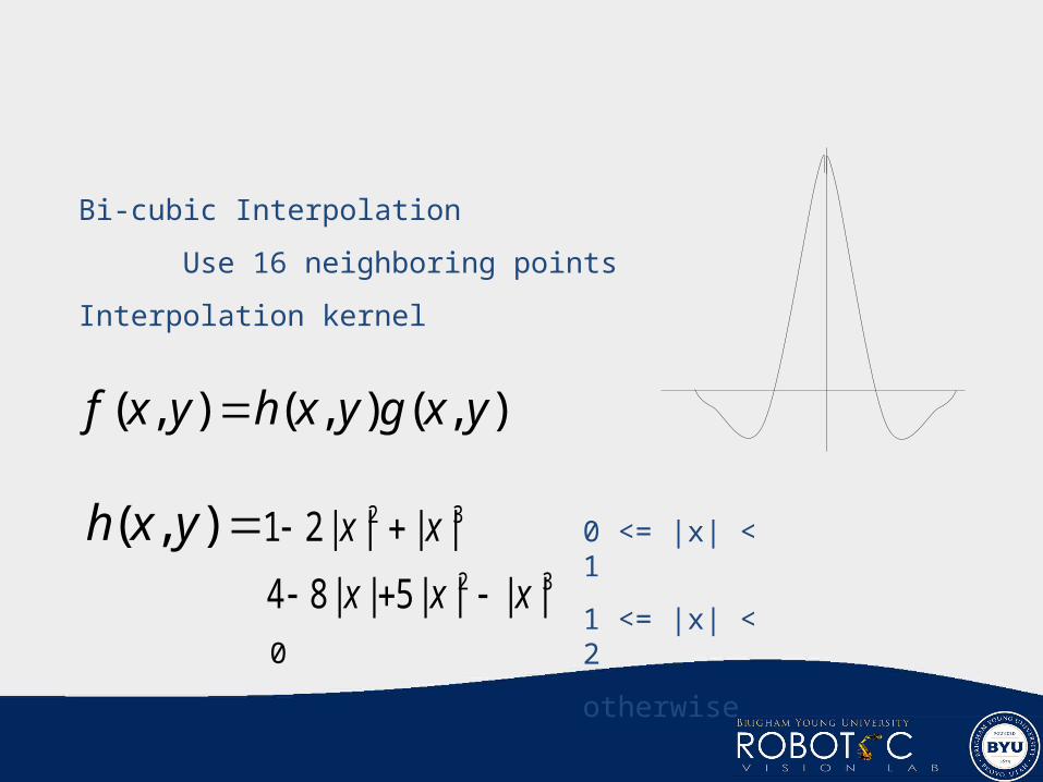
Bi-cubic Interpolation
Use 16 neighboring points
Interpolation kernel
),(),(),( yxgyxhyxf
32
32
||||5||84
||||21
xxx
xx
),( yxh 0 <= |x| < 1
1 <= |x| < 2
otherwise0