ieee transactions on plasma science, submitted 1 power

IEEE TRANSACTIONS ON PLASMA SCIENCE, SUBMITTED 1

Power Deposition on Tokamak Plasma-FacingComponents

Wayne Arter, Member, IEEE, Valeria Riccardo and Geoff Fishpool

Abstract—The SMARDDA software library is used to modelplasma interaction with complex engineered surfaces. A simpleflux-tube model of power deposition necessitates the following ofmagnetic fieldlines until they intersect geometry taken from aCAD (Computer Aided Design) database. Application is madeto 1) models of ITER tokamak limiter geometry and 2) MAST-U tokamak divertor designs, illustrating the accuracy and ef-fectiveness of SMARDDA, even in the presence of significantnonaxisymmetric ripple field. SMARDDA’s ability to exchangedata with CAD databases and its speed of execution also give itthe potential for use directly in the design of tokamak plasma-facing components.

I. INTRODUCTION

THE problem of economic electrical power generationusing tokamak nuclear fusion continues to generate new

technological challenges, even as the basic issues involvedin magnetically confining plasma become better understood.Tokamak reactor designs anticipate long periods, months toyears in length, of continuous plasma discharge operation atpowers of up to 2 GW. Helium “ash” produced by fusion thatcould otherwise prematurely terminate a discharge must becontinually removed from the edge, most likely taking withit a significant fraction of the total plasma power. Even inlarge tokamak experiments, the deposition of plasma energylost from the edge onto likely construction materials hasthe potential to do serious structural damage if restricted torelatively small areas of the size of the plasma “scrape-off”layer with its 1 cm or so thickness.

Plasma-facing component (PFC) is a generic term for anypart of the tokamak apparatus which could conceivably suffera significant amount of power deposition. The main types arelimiters, that are at least in part touching the plasma edge(see Figure 6 in Section III for illustration), and divertors, intowhich escaping plasma is channeled to be cooled and/or spreadout (see Figure 11 in Section IV) and which are expected to bean essential component of a power-producing reactor. In eithercase the physical objects interacting with plasma consist ofpanels or tiles made of or at least coated with refractory metal,protecting complex structures that for example provide activecooling. Although greater interest attaches to power handlingin divertors, most scenarios for tokamak discharge start-upinvolve a period of limiter operation with a comparativelyenergetic plasma.

W. Arter, V. Riccardo and G. Fishpool are employed by the UnitedKingdom Atomic Energy Authority, EURATOM/CCFE Fusion Association,Culham Science Centre, Abingdon, Oxon. UK OX14 3DB e-mail: (seehttp://www.ccfe.ac.uk).

Manuscript received XXXX.

This paper shows how a relatively small development ofthe software algorithms and modules described for a neutralbeam application in companion Paper I [1] has allowed theSMARDDA code to examine power deposition in both limiterand divertor geometries. The limiter studies were in support ofITER [2], whereas divertor designs were tested for the upgradeof the MAST spherical tokamak at Culham [3]. Althoughin both cases, SMARDDA was used to verify engineeringdesigns produced by others, the speed of execution of thesoftware would enable it to be more directly involved thedesign process.

A. Power deposition problem

Since the edge plasma is relatively cool, indicative temper-ature 10 eV, yet the field is relatively high, indicative level 5 T(in ITER), the typical ion gyro-radius is very small, 100µmcompared to a plasma minor radius measured in metres.Hence, as a consequence of the individual motions of thecharged particles (ignoring turbulent collective effects), theplasma that interacts with PFCs simply flows along lines ofmagnetic field. To spread the power over as large an areaas possible, it is therefore best to arrange the PFCs so thatmagnetic fieldlines are at close to tangential incidence on theirsurfaces, see formulae for power deposition Q in Section II-B.

For a given field alignment and shallow angle of incidence,designing individual tile surfaces is relatively straightfor-ward [4]. However, this is not a complete answer, in thatfirstly the fieldlines are are not strictly straight and secondly,the actual installation may differ substantially from the ideal,notably through the presence of gaps, and installation toler-ances will allow minor misalignments. The gaps, where powermight flow between the tiles/panels, are necessary to giveclearances for installation and to allow for thermal expansionduring discharges. Since the edges of the tiles, ie. thosesurfaces adjacent to the designed surfaces, are at nearly normalincidence to the field, they might have very high levels ofpower deposition unless nearby tiles were arranged to shadowthem. However, it is also important to minimise the shadowingof one designed surface by another as shadowing increasesoverall average power density.

Further, particularly within a divertor geometry, it may benecessary to allow for fieldline curvature and ripple, whereasfor limiters, it may be necessary to treat a range of differentfield alignments, corresponding to different types of dischargesand different times within a discharge. Hence there is theneed for software which can examine detailed designs of setsof tiles, ultimately defined using a CAD (Computer Aided

arX

iv:1

403.

7142

v2 [

phys

ics.

plas

m-p

h] 5

Apr

201

6

http://www.ccfe.ac.uk


Design) system, and their interaction with an accurate 3-Drepresentation of the magnetic field.

B. SMARDDA

As described in the companion Paper I [1], the SMARDDAsoftware was developed to have in principle all of the fea-tures necessary to perform design-relevant calculations forPFCs. Ancillary software takes geometry modelled using theCATIATM design system and converts it to the “open” vtkformat [5] expected by the main modules, which describes thegeometry as triangulated surfaces. Charged particles, producedby charge exchange reactions between a neutral beam andplasma in a duct, are tracked in a magnetic field until theystrike the duct walls, and the resulting power deposition isexamined. SMARDDA uses a specially designed algorithminvolving a special multi-octree type of hierarchical datastructure (HDS) to speed particle tracking.

However, it is very inefficient to track particle motionsdirectly when they anyway closely follow magnetic fieldlines,so development was necessary to solve the stream- or fieldlineequation of motion. In addition, new formulae for powerdeposition are required when it is the local magnetic flux tubethat is responsible for the process, and new ways are needed tointroduce “particles” into the model to represent the fieldlines.

Fortunately, the original SMARDDA development benefit-ted from the use of Object-Oriented Fortran in its implemen-tation, which mandates use of strictly defined and protectedobjects, hence a modular structure of code. The concept thusnaturally developed that SMARDDA should become muchmore a library of object-oriented modules from which codesfor specific purposes could be built as necessary. The originalHDSGEN software written to generate the HDS needed forSMARDDA ray-tracing exemplifies such a code.

Many codes have been written to track streamlines of fluidflow, and indeed the facility is available in the freely availableParaView software [6] used for the visualisation of vtk filesand indeed for much SMARDDA output. However, the re-quirement for streamlines to intersect surfaces is more unusual,and to meet this only literature involving magnetic fields seemsto be relevant. Particle-in-Cell (PIC) codes were discussedin Paper I, and as for codes designed specifically to followfieldlines, most are either not interested in wall interactions ormodel them with idealised geometry. The only documentedcode with the capability to treat realistic CAD designs atthe time of the SMARDDA development was Tokaflu [7],but this has a number of deficiencies, notably in respect ofcomputational efficiency. The authors of the general-purposeISDEP particle tracking software [8] do not explain how ittreats complex geometry. Very recently a module has beenadded to the magnetic field equilibrium software CREATE inorder to track fieldlines over triangulated geometry [9].

The new developments are discussed in the context of theuse of SMARDDA to perform the different modelling tasks,see next Section II-A.

II. GENERAL METHODS OF CALCULATION

A. Introduction

For both limiter and divertor cases, the geometry is logicallydivided into two types, the first is the part for which powerdeposition is to be calculated (the “results” geometry) and thesecond type is the geometry which protects the edges of thefirst by fieldline shadowing (the “shadowing geometry”). Animportant practical point is where to start the fieldlines, andfor efficiency it seems best to adopt the “adjoint” concept fromcomputer graphics, namely to begin the fieldlines on the resultsgeometry, and test whether they can be followed to the nominalsource of power at the tokamak midplane without striking theshadowing geometry. Hence the “results” geometry may alsobe referred to as the “launch” geometry, contrast Paper I whereparticles are launched to sample analytically defined beamletsand power is deposited on the shadowing geometry.

Figure 1 outlines the flow of data needed to calculatepower deposition on limiter tiles/panels (the data-flow for thedivertor case is very similar). The import of CAD (top left)using the CADfixTM package supplied by ITI TranscenData isdiscussed in detail in Paper I. Locally written software convertsa CADfix mesh for either results or shadowing geometry intovtk format at the point labelled “x mesh” in Figure 1, seeSection II-C below for more details. “EQDSK” file (top right)denotes a file format which describes a tokamak magneticfield equilibrium. Glasser’s DCON code [10] may optionallybe used to check the contents of the EQDSK file, or actas an interface to other equilibrium field file formats. Themagnetic field B is assumed to be axisymmetric, independentof toroidal angle φ, and thus can be described by a (poloidal)flux function ψ, together with a toroidal component specifiedby the flux function I(ψ).

In the limiter case, fieldline calculation takes place in acoordinate frame aligned with contours of ψ. Geometry andequilibrium data is combined by the GEOQ code to givethe “xψ mesh” file which has the geometrical informationin flux coordinates, see Section II-D below. The HDSGENcode, described in Paper I is shown in the red box to indicatethat it is only required for processing the shadowing geometry.Although it is apparently thereby implicitly assumed that the“results” geometry cannot be struck by a fieldline, the same tiletriangulation can in fact be part of both launch and shadowinggeometry.

The fieldline tracing and power deposition calculations arethen performed by the POWRES code, or the POWCAL codein the case of divertor calculations. The latter follows fieldlinesusing cylindrical polar coordinates in physical space. Featurescommon to both codes are described in the remainder ofthis Section, starting with the power deposition model as thisinforms subsequent material which is ordered after the flow ofFigure 1. Model features and files specific to the treatment ofnonaxisymmetric “ripple” field are described in Section IV.

B. Model of Power Deposition

A simple model of power deposition by plasma in flux tubesis used in calculations of the tokamak edge. Since it doesnot seem to have been fully documented elsewhere, details of


Fig. 1. The flow of data through the SMARDDA modules for limiterproblems.

Fig. 2. Flux tube of field B connecting the torus midplane with a surfaceindicated schematically in grey with normal n. The flux tube area is A1 atbottom right, at top left it is cut by a horizontal circle with area A0.

the derivation of the principal formula are presented in theAppendix A. The basic idea may be explained using Figure 2,which shows a flux-tube connecting the tokamak mid-planewith a physical surface of area A1. As it is assumed thatparticles follow fieldlines, all power entering the top of thetube strikes the surface at bottom. Further, the power at thetop of the tube is assumed to fall off exponentially with (major)radial distance at an empirically determined rate λm from thelast closed flux surface (LCFS) [11]. The LCFS is given byψ = ψm where ψm is the value of the poloidal flux where thegeometry touches the plasma, or equal to ψ at the X-point incase of divertor plasmas. In Appendix A, the power density Qdeposited on the PFC is shown to vary as

Q = CstdB · n exp

(− (ψ − ψm)

λmRmBpm

)(1)

where ψ is the flux function value for the tube at the mid-plane,and the other quantities including the power normalisationfactor Cstd (see Appendix A) are fixed for a given equilibriumand geometry. The formula is found to be a very accurate fitfor suitably chosen λm to data from many different tokamakexperiments [12].

1) Eich formula for Power Deposition: Eich’s formula[13] is relevant only to divertor geometries. It accounts forthe spread of power into the “private flux” region of thedivertor, apparently caused by some kind of collective plasmabehaviour. Relative to the previous formula Eq. (1), there isan additional parameter σ to describe the fall-off length forpower deposited in the private flux region, so that Q variessmoothly across the surface ψ = ψm, as

QE = CEB · n exp

[(σ

2λq

)2

− ∆ψ

RmBpmλq

]FE(ψ) (2)

whereFE(ψ) = erfc

(σ

2λq− ∆ψ

RmBpmσ

)(3)

andCE =

FPloss4πRmλqBpm

(4)

In the above, ∆ψ = ψ − ψm, λq now denotes the char-acteristic decay length outside the private flux region, andother quantities are as defined in Appendix A. Despite itsformidable appearance QE(ψ) is analytically integrable andthe normalisation is exact.

C. Meshing and Mesh Refinement

1) Meshing: It is generally sufficient for limiter plasmasto consider shadowing by adjacent panels only, as confirmedby SMARDDA calculations with the ITER geometry, seeSection III. This is not necessarily true for divertor plasmas,but for the MAST-U work there is the simplification that thedivertor design has twelve-fold symmetry about the major axis.Hence in both cases, the region to be meshed is reduced toa small fraction of the total limiter/divertor area, since thereare some 360 panels in ITER designs (cf. over 100 tiles inMAST-U divertor).

A major saving both in user and computer time isachieved by only meshing the surfaces of PFCs. For MAST-U, compared to the typical tile or panel surface dimensionsof 30 cm×1 m, the inter-tile gaps are approximately 2 mm.This implies that to verify absence of power deposition onthe tile edges, triangles with a side of order this length will berequired. A uniform meshing at 2 mm is excessive in requiringover 105 triangles per tile, so it is economical to produce asurface mesh which grades down to this size only in the criticalareas, as elsewhere a 30 mm spacing is sufficient, at least forexploratory calculations, see Section III and Section IV.

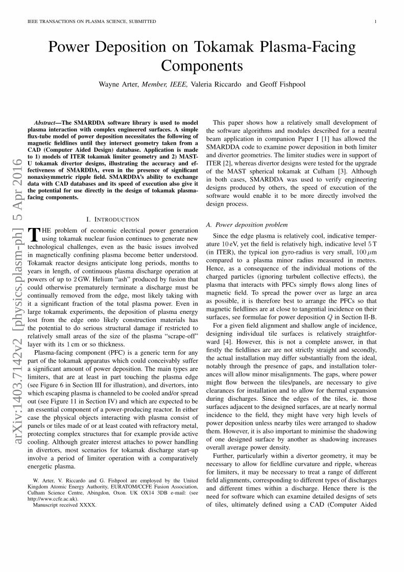
2) Automatic Mesh Refinement: One unique feature of theCADfixTM package used for the meshing is its FORTRANAPI (Application Programmer Interface). This API has beenused in the development of the CFMCN code capable notonly of generating the vtk files describing triangulations, butalso to produce a succession of refinements automatically fora given triangulation. Each triangle is separately divided intofour as indicated in Figure 3 with the important feature that thesplitting points are geometry-conforming, ie. they lie on theCAD surface and are not just averages of pre-existing points.This ability to produce meshes at ×4 and ×16 resolution ismost helpful for convergence studies.


Fig. 3. This illustrates the subdivision of a triangle into four congruentparts by geometry-conforming points which is performed automatically bythe CFMCN code.

3) Surface Accuracy: For the most part, it is the shadowingof PFC surfaces which is the main issue. However, sincepower deposition Q ∝ B · n with B arranged to be nearlyperpendicular to n, if accurate numerical values are needed, itis necessary to be able to reproduce the surface normal direc-tion accurately. The economical approach to data adopted bySMARDDA relies on approximating the tile normal using thenormals of the triangular facetting, rather than say augmentingthe triangulation file with n values extracted from the CADdatabase. The consequent error in Bn = B ·n is examined indetail in Appendix B for a simple configuration of a toroidalfield intersecting a vertical cone of apex angle π/2− α.

Assuming that beyond a certain major radius, the cone ismeshed with “Union Jacks” as explained in Appendix B, thenthe surface normal computed using plane triangular facets oftoroidal angular extent ∆φ has a component in the toroidaldirection equal to (∆φ/2) sinα. (The factor of 1

2 arisesultimately because two edges define the normal.) However thelogical place to calculate Bn is at the triangle barycentre wherethe geometry-conforming normal is found to contain a factorof 1

3 , leading to an error in Q scaling as ∆Q ∝ (∆φ/6) sinα.The “Union Jack” mesh, although pleasing to the eye, isactually here very bad for ∆Q. Even so, the linear scalingof error with mesh-spacing is likely to apply for most stylesof triangulation, and accounts for the irregular appearance ofQ plots on the (coarse) base meshes seen in later sections.

D. Magnetic Field Import

For input to GEOQ (Figure 1), different ITER field dis-tributions are specified using EQDSK files produced by theCREATE-NL software from the Consortio CREATE [14],whereas equivalent files for MAST-U work are produced bythe locally written Fiesta code [15]. The file format specifiesψ as a set of values on a regularly spaced grid in (R,Z).Direct product cubic spline interpolation of the sample valuesand their derivatives using the de Boor package [16] is usedin the obvious way to define the magnetic field at any pointin the gridded region.

Once the flux has been interpolated, it is straightforward tocalculate ψm for the limiter plasmas. To determine other pa-rameters such as Rm and ψm for X-point plasmas, it is helpfulto work in the coordinate system given by ψ and θ, poloidalangle measured about the O-point in the centre (Rcen, Zcen) ofthe plasma. Use of an analytically defined coordinate such as θ

reduces these other parameter determinations to a sequence of1-D golden-section searches, each in the radial or ψ-direction.

Since the ITER calculations work directly with (ψ, θ) fluxcoordinates, it is necessary to calculate the (inverse) mappingfunctions R(ψ, θ) and Z(ψ, θ). Fortunately for limiter calcu-lations, these are only needed at such a distance from theX-point that both are well-behaved functions of ψ. They arecalculated point-by-point in much the same way as the otherparameters, ie. for each point (ψi, θj) of a regular lattice influx coordinates, a search is conducted along the radius θ = θjto find (Ri, Zj) such that ψ(Ri, Zj) = ψi. Cubic splines areused throughout to ensure good accuracy, which is tested bycombining a forward with a backwards mapping, ie. using(R,Z) evaluated at (ψi, θj) as argument to ψ(R,Z), andverifying that |ψ − ψi| is accurate to at least 1 part in 104.

E. Fieldline tracing

In terms of ψ and I(ψ), the magnetic field components incylindrical polars are

BR = − 1

R

∂ψ

∂ZBT = I/R (5)

BZ =1

R

∂ψ

∂R

where BT is the toroidal component of field, directed in theφ coordinate. The standard fieldline equation is

x =dx

dt= B(x) (6)

where dot denotes differentiation with respect to pseudo-time tmeasured along the fieldline. For time independent fields itmay be helpful to think of t as corresponding to fieldlinelength. When flux coordinates are used, Eq. (6) simplifies to

dθ

dφ= (1/I)R/J(ψ, θ) (7)

where J(ψ, θ) is the Jacobian of the mapping transformation.Although the computational costs of solving the ordinary

differential equations (ODEs) of Eq. (6) are usually negligibleon modern hardware, it is still important to choose a numericalalgorithm tailored to present requirements, namely

1) Relatively inexpensive, because 103–105 or more field-lines will need to be computed, corresponding the sizeof triangulation of the results geometry.

2) Millimetre accuracy in following fieldlines, correspond-ing to the expected accuracy in the position of PFCssubject to thermal expansion effects.

3) Step sizes such that the fieldline is approximatelystraight over one step in t, to ensure accurate geometryintersection.

These requirements are most easily met by a low orderscheme with adaptive timestepping to ensure (2). Runge-Kutta-Fehlberg (RKF) also known as (aka) Embedded Runge-Kuttaschemes with step adaptation by the Shampine-Watts [17] akaCash-Karp algorithm are well documented and relatively easyto implement. There is however a further restriction on order ofaccuracy, for Shampine-Watts relies on a degree of smoothness


of the solution x(t) at least that of the RKF scheme inorder to estimate accurately the error in the integration. As iswell-known, cubic splines have discontinuous third derivative,hence is sensible to use third order RKF. Details of the specificschemes implemented are presented in Appendix C.

F. Diagnostics

The diagnostics produced by the SMARDDA codes will beadequately exhibited by plots in Section III and Section IV.Output suitable for the open source plotting tool gnuplot isproduced by GEOQ, and all plots of 3-D fields unsurprisinglyuse the vtk format to be visualised with ParaView [19].Moreover, ParaView can perform a wide range of analyses offield data, which give it the capability for example, to calculatethe total power deposited on a tile from the contributions ofindividual elements.

III. APPLICATION TO ITER

A. Background

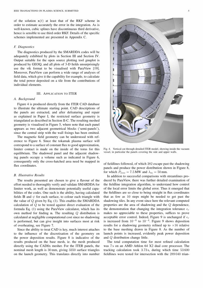
Figure 4 is produced directly from the ITER CAD databaseto illustrate the ultimate starting point. CAD descriptions ofthe panels are extracted, and after defeaturing and repairas explained in Paper I, the restricted surface geometry istriangulated as described in Section II-C. The resulting meshedgeometry is visualised in Figure 5, where note that each panelappears as two adjacent geometrical blocks (‘semi-panels’),since the central strip with the wall fixings has been omitted.

The magnetic field geometry can be understood with ref-erence to Figure 6. Since the tokamak plasma surface willcorrespond to a surface of constant flux to good approximation,limiter contact is made on the inside of the torus for thisequilibrium. The shadowed panel and the adjacent shadow-ing panels occupy a volume such as indicated in Figure 6,consequently only the cross-hatched area need be mapped influx coordinates.

B. Illustrative Results

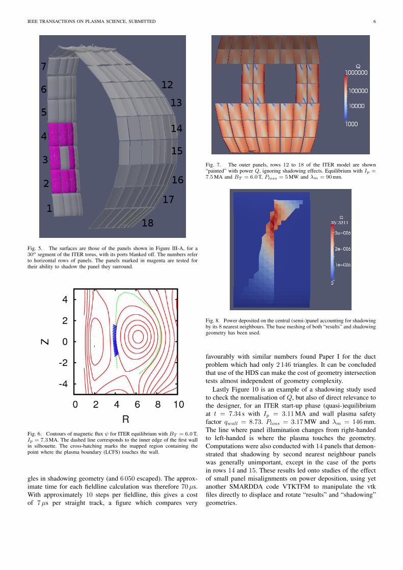
The results presented are chosen to give a flavour of theeffort needed to thoroughly verify and validate SMARDDA forlimiter work, as well as demonstrate potentially useful capa-bilities of the codes. One such is the ability, having calculatedfields B and ψ for each surface, to colour each triangle withthe value of Q given by Eq. (1). This enables the SMARDDAcalculation of Q to be tested against direct evaluation of theformula Eq. (1) using the ParaView calculator, which has itsown method for finding n. The resulting Q distribution iscalculated at negligible computational cost since no shadowingis performed, but can give insight into surfaces most at riskof overheating, see Figure 7.

Since the ability to treat CAD is key, much interest attachesto the influence of the discretisation of the geometry onthe power deposition results. Figure 8 is indicative of theresults produced on the base mesh, ie. the mesh produceddirectly using the CADfix mesher. For the ITER panels, thenominal mesh length is 30 mm, giving 3350 surface triangleson the launch geometry. This translates directly into number

Fig. 4. Vertical cut through detailed ITER model, showing inside the vacuumvessel, in particular the panels covering the side and upper walls.

of fieldlines followed, of which 382 escape past the shadowingpanels and produce the power distribution shown in Figure 8,for which Ploss = 7.5 MW and λm = 50 mm.

In addition to successful comparisons with streamlines pro-duced by ParaView, there was further detailed examination ofthe fieldline integration algorithm, to understand how controlof the local error limits the global error. Thus it emerged thatthe fieldlines are so close to being straight in flux coordinatesthat as few as 10 steps might be needed to get past theshadowing tiles. In any event since here the relevant computedproperties are the area of shadowing and the Q dependence,the demonstration that changing the integration tolerance εrmakes no appreciable to these properties, suffices to proveacceptable error control. Indeed, Figure 9 is unchanged if εris increased from 10−6 to 10−4. Figure 9 shows depositionresults for a shadowing geometry refined up to ×16 relativeto the base meshing drawn in Figure 8. As the number oflaunch points is increased, evidently peak power depositionand Q distribution change little.

The total computation time for most refined calculationwas 7 s on an AMD Athlon 64 X2 dual core processor. Thetracking calculation took 3.73 s, during which time 53 600fieldlines were tested for intersection with the 289 040 trian-


Fig. 5. The surfaces are those of the panels shown in Figure III-A, for a30o segment of the ITER torus, with its ports blanked off. The numbers referto horizontal rows of panels. The panels marked in magenta are tested fortheir ability to shadow the panel they surround.

Fig. 6. Contours of magnetic flux ψ for ITER equilibrium with BT = 6.0T,Ip = 7.3MA. The dashed line corresponds to the inner edge of the first wallin silhouette. The cross-hatching marks the mapped region containing thepoint where the plasma boundary (LCFS) touches the wall.

gles in shadowing geometry (and 6 050 escaped). The approx-imate time for each fieldline calculation was therefore 70µs.With approximately 10 steps per fieldline, this gives a costof 7µs per straight track, a figure which compares very

Fig. 7. The outer panels, rows 12 to 18 of the ITER model are shown“painted” with power Q, ignoring shadowing effects. Equilibrium with Ip =7.5MA and BT = 6.0T, Ploss = 5MW and λm = 90mm.

Fig. 8. Power deposited on the central (semi-)panel accounting for shadowingby its 8 nearest neighbours. The base meshing of both “results” and shadowinggeometry has been used.

favourably with similar numbers found Paper I for the ductproblem which had only 2 146 triangles. It can be concludedthat use of the HDS can make the cost of geometry intersectiontests almost independent of geometry complexity.

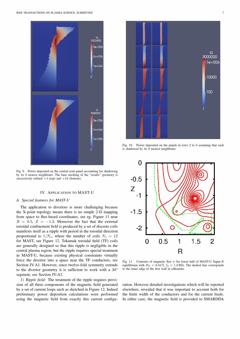
Lastly Figure 10 is an example of a shadowing study usedto check the normalisation of Q, but also of direct relevance tothe designer, for an ITER start-up phase (quasi-)equilibriumat t = 7.34 s with Ip = 3.11 MA and wall plasma safetyfactor qwall = 8.73. Ploss = 3.17 MW and λm = 146 mm.The line where panel illumination changes from right-handedto left-handed is where the plasma touches the geometry.Computations were also conducted with 14 panels that demon-strated that shadowing by second nearest neighbour panelswas generally unimportant, except in the case of the portsin rows 14 and 15. These results led onto studies of the effectof small panel misalignments on power deposition, using yetanother SMARDDA code VTKTFM to manipulate the vtkfiles directly to displace and rotate “results” and “shadowing”geometries.


Fig. 9. Power deposited on the central semi-panel accounting for shadowingby its 8 nearest neighbours. The base meshing of the “results” geometry issuccessively refined ×4 (top) and ×16 (bottom).

IV. APPLICATION TO MAST-U

A. Special features for MAST-U

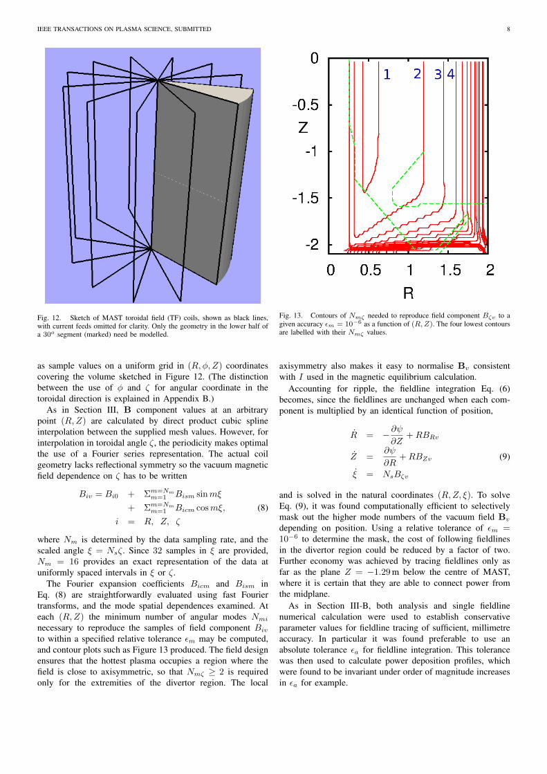
The application to divertors is more challenging becausethe X-point topology means there is no simple 2-D mappingfrom space to flux-based coordinates, see eg. Figure 11 nearR = 0.5, Z = −1.3. Moreover the fact that the externaltoroidal confinement field is produced by a set of discrete coilsmanifests itself as a ripple with period in the toroidal directionproportional to 1/Ns, where the number of coils Ns = 12for MAST, see Figure 12. Tokamak toroidal field (TF) coilsare generally designed so that this ripple is negligible in thecentral plasma region, but the ripple requires special treatmentin MAST-U, because existing physical constraints virtuallyforce the divertor into a space near the TF conductors, seeSection IV-A1. However, since twelve-fold symmetry extendsto the divertor geometry it is sufficient to work with a 30o

segment, see Section IV-A2.1) Ripple field: The treatment of the ripple requires provi-

sion of all three components of the magnetic field generatedby a set of current loops such as sketched in Figure 12. Indeedpreliminary power deposition calculations were performedusing the magnetic field from exactly this current configu-

Fig. 10. Power deposited on the panels in rows 2 to 6 assuming that eachis shadowed by its 8 nearest neighbours.

Fig. 11. Contours of magnetic flux ψ for lower half of MAST-U Super-Xequilibrium with BT = 0.64T, Ip = 1.0MA. The dashed line correspondsto the inner edge of the first wall in silhouette.

ration. However detailed investigations which will be reportedelsewhere, revealed that it was important to account both forthe finite width of the conductors and for the current feeds.In either case, the magnetic field is provided to SMARDDA


Fig. 12. Sketch of MAST toroidal field (TF) coils, shown as black lines,with current feeds omitted for clarity. Only the geometry in the lower half ofa 30o segment (marked) need be modelled.

as sample values on a uniform grid in (R,φ, Z) coordinatescovering the volume sketched in Figure 12. (The distinctionbetween the use of φ and ζ for angular coordinate in thetoroidal direction is explained in Appendix B.)

As in Section III, B component values at an arbitrarypoint (R,Z) are calculated by direct product cubic splineinterpolation between the supplied mesh values. However, forinterpolation in toroidal angle ζ, the periodicity makes optimalthe use of a Fourier series representation. The actual coilgeometry lacks reflectional symmetry so the vacuum magneticfield dependence on ζ has to be written

Biv = Bi0 + Σm=Nmm=1 Bism sinmξ

+ Σm=Nmm=1 Bicm cosmξ, (8)

i = R, Z, ζ

where Nm is determined by the data sampling rate, and thescaled angle ξ = Nsζ. Since 32 samples in ξ are provided,Nm = 16 provides an exact representation of the data atuniformly spaced intervals in ξ or ζ.

The Fourier expansion coefficients Bicm and Bism inEq. (8) are straightforwardly evaluated using fast Fouriertransforms, and the mode spatial dependences examined. Ateach (R,Z) the minimum number of angular modes Nminecessary to reproduce the samples of field component Bivto within a specified relative tolerance εm may be computed,and contour plots such as Figure 13 produced. The field designensures that the hottest plasma occupies a region where thefield is close to axisymmetric, so that Nmζ ≥ 2 is requiredonly for the extremities of the divertor region. The local

Fig. 13. Contours of Nmζ needed to reproduce field component Bζv to agiven accuracy εm = 10−6 as a function of (R,Z). The four lowest contoursare labelled with their Nmζ values.

axisymmetry also makes it easy to normalise Bv consistentwith I used in the magnetic equilibrium calculation.

Accounting for ripple, the fieldline integration Eq. (6)becomes, since the fieldlines are unchanged when each com-ponent is multiplied by an identical function of position,

R = −∂ψ∂Z

+RBRv

Z =∂ψ

∂R+RBZv (9)

ξ = NsBζv

and is solved in the natural coordinates (R,Z, ξ). To solveEq. (9), it was found computationally efficient to selectivelymask out the higher mode numbers of the vacuum field Bv

depending on position. Using a relative tolerance of εm =10−6 to determine the mask, the cost of following fieldlinesin the divertor region could be reduced by a factor of two.Further economy was achieved by tracing fieldlines only asfar as the plane Z = −1.29 m below the centre of MAST,where it is certain that they are able to connect power fromthe midplane.

As in Section III-B, both analysis and single fieldlinenumerical calculation were used to establish conservativeparameter values for fieldline tracing of sufficient, millimetreaccuracy. In particular it was found preferable to use anabsolute tolerance εa for fieldline integration. This tolerancewas then used to calculate power deposition profiles, whichwere found to be invariant under order of magnitude increasesin εa for example.


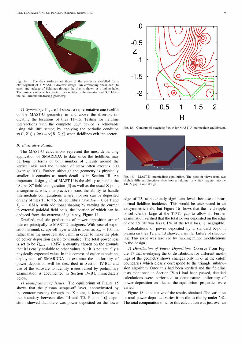
Fig. 14. The dark surfaces are those of the geometry modelled for a30o segment of a MAST-U divertor design. An enveloping “bean-can” tocatch any leakage of fieldlines through the tiles is shown as a lighter halo.The numbers refer to horizontal rows of tiles in the divertor and “C” labelsthe coil armour shadowing geometry.

2) Symmetry: Figure 14 shows a representative one-twelfthof the MAST-U geometry in and above the divertor, in-dicating the locations of tiles T1–T5. Testing for fieldlineintersections with the complete 360o device is achievableusing this 30o sector, by applying the periodic conditionx(R,Z, ξ + 2π) = x(R,Z, ξ) when fieldlines exit the sector.

B. Illustrative Results

The MAST-U calculations represent the most demandingapplication of SMARDDA to date since the fieldlines maybe long in terms of both number of circuits around thevertical axis and the number of steps often exceeds 500(average 100). Further, although the geometry is physicallysmaller, it contains as much detail as in Section III. Animportant design goal of MAST-U is the ability to handle the“Super-X” field configuration [3] as well as the usual X-pointarrangement, which in practice means the ability to handleintermediate configurations wherein power can be depositedon any of tiles T1 to T5. All equilibria have BT = 0.64 T andIp = 1.0 MA, with additional shaping by varying the currentin external poloidal field coils, the location of which can bededuced from the extrema of ψ in say, Figure 11.

Detailed, realistic predictions of power deposition are ofinterest principally to MAST-U designers. With ease of expo-sition in mind, scrape-off layer width is taken as λm = 10 mm,rather than the more realistic 3 mm in order to make the plotsof power deposition easier to visualise. The total power lossis set to be Ploss = 1 MW, a quantity chosen on the groundsthat it is easily scalable to other values, but it is not actually aphysically expected value. In this context of easier exposition,deployment of SMARDDA to examine the uniformity ofpower deposition will be described in Section IV-B2, anduse of the software to identify issues raised by preliminaryexamination is documented in Section IV-B1, immediatelybelow.

1) Identification of Issues: The equilibrium of Figure 15shows that the plasma scrape-off layer, approximated bythe contour passing through the X-point, is located close tothe boundary between tiles T4 and T5. Plots of Q depo-sition showed that there was power deposited on the lower

Fig. 15. Contours of magnetic flux ψ for MAST-U intermediate equilibrium.

Fig. 16. MAST-U intermediate equilibrium. The plots of views from twoslightly different directions show how a fieldline (in white) may get into theT4/T5 gap in one design.

edge of T5, at potentially significant levels because of near-normal fieldline incidence. This would be unexpected in anaxisymmetric field, but Figure 16 shows that the field rippleis sufficiently large at the T4/T5 gap to allow it. Furtherexamination verified that the total power deposited on the edgeof one T5 tile was less 0.1 % of the total loss, ie. negligible.

Calculations of power deposited by a standard X-pointplasma on tiles T2 and T3 showed a similar failure of shadow-ing. This issue was resolved by making minor modificationsto the design.

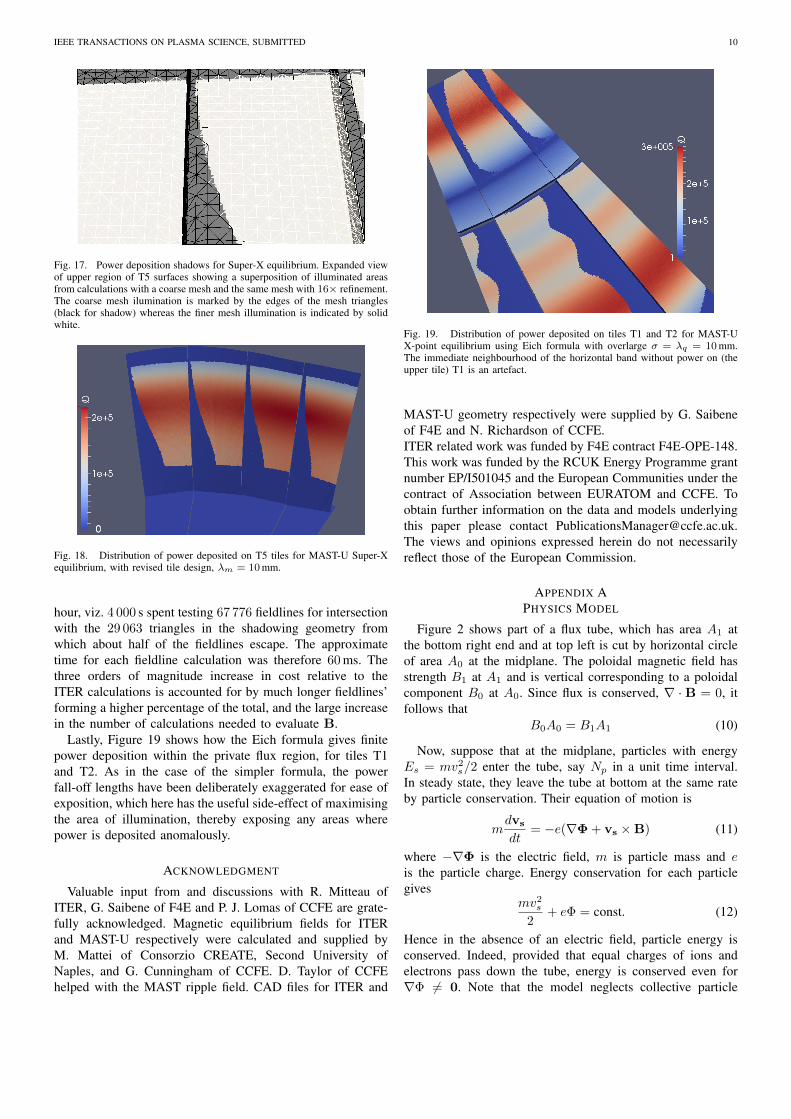
2) Distribution of Power Deposition: Observe from Fig-ure 17 that overlaying the Q distributions for different mesh-ings of the geometry shows changes only in Q at the cutoffboundaries which clearly correspond to the triangle subdivi-sion algorithm. Once this had been verified and the fieldlinetests mentioned in Section IV-A1 had been passed, detailedcalculations were performed to demonstrate uniformity ofpower deposition on tiles as the equilibrium properties werevaried.

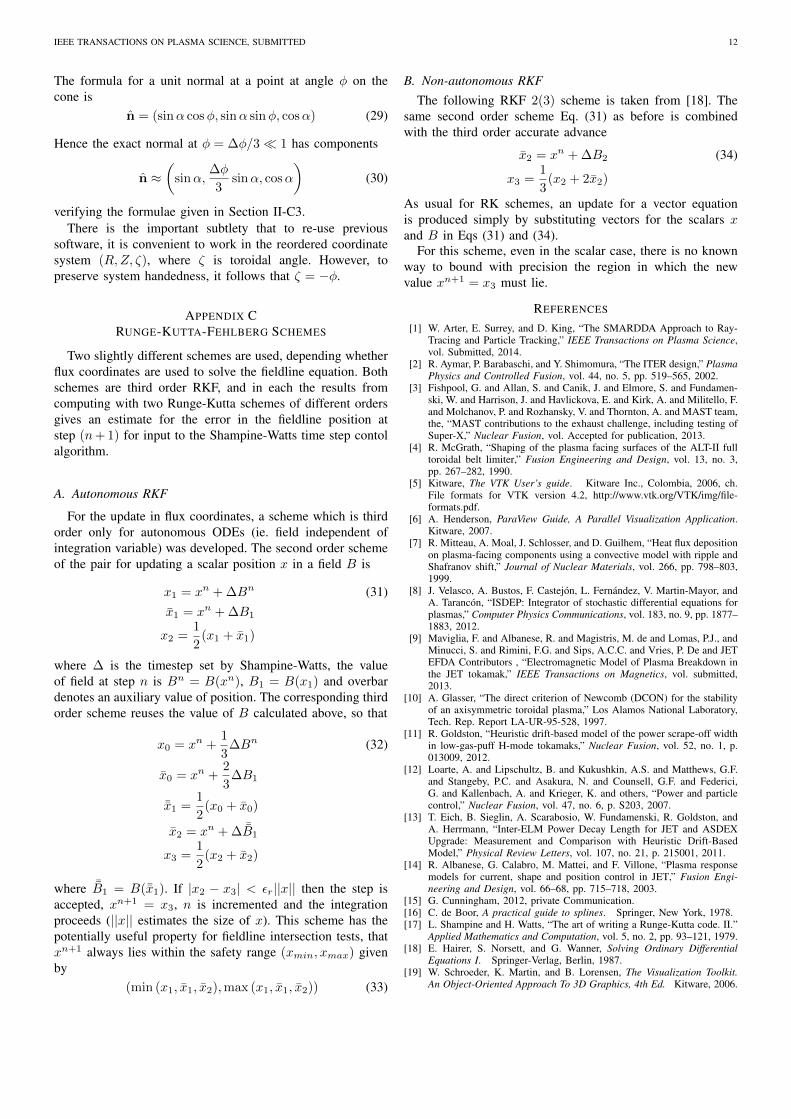
Figure 18 is indicative of the results obtained. The variationin total power deposited varies from tile to tile by under 5 %.The total computation time for this calculation was just over an


Fig. 17. Power deposition shadows for Super-X equilibrium. Expanded viewof upper region of T5 surfaces showing a superposition of illuminated areasfrom calculations with a coarse mesh and the same mesh with 16× refinement.The coarse mesh ilumination is marked by the edges of the mesh triangles(black for shadow) whereas the finer mesh illumination is indicated by solidwhite.

Fig. 18. Distribution of power deposited on T5 tiles for MAST-U Super-Xequilibrium, with revised tile design, λm = 10mm.

hour, viz. 4 000 s spent testing 67 776 fieldlines for intersectionwith the 29 063 triangles in the shadowing geometry fromwhich about half of the fieldlines escape. The approximatetime for each fieldline calculation was therefore 60 ms. Thethree orders of magnitude increase in cost relative to theITER calculations is accounted for by much longer fieldlines’forming a higher percentage of the total, and the large increasein the number of calculations needed to evaluate B.

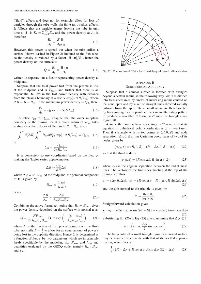
Lastly, Figure 19 shows how the Eich formula gives finitepower deposition within the private flux region, for tiles T1and T2. As in the case of the simpler formula, the powerfall-off lengths have been deliberately exaggerated for ease ofexposition, which here has the useful side-effect of maximisingthe area of illumination, thereby exposing any areas wherepower is deposited anomalously.

ACKNOWLEDGMENT

Valuable input from and discussions with R. Mitteau ofITER, G. Saibene of F4E and P. J. Lomas of CCFE are grate-fully acknowledged. Magnetic equilibrium fields for ITERand MAST-U respectively were calculated and supplied byM. Mattei of Consorzio CREATE, Second University ofNaples, and G. Cunningham of CCFE. D. Taylor of CCFEhelped with the MAST ripple field. CAD files for ITER and

Fig. 19. Distribution of power deposited on tiles T1 and T2 for MAST-UX-point equilibrium using Eich formula with overlarge σ = λq = 10mm.The immediate neighbourhood of the horizontal band without power on (theupper tile) T1 is an artefact.

MAST-U geometry respectively were supplied by G. Saibeneof F4E and N. Richardson of CCFE.ITER related work was funded by F4E contract F4E-OPE-148.This work was funded by the RCUK Energy Programme grantnumber EP/I501045 and the European Communities under thecontract of Association between EURATOM and CCFE. Toobtain further information on the data and models underlyingthis paper please contact [email protected] views and opinions expressed herein do not necessarilyreflect those of the European Commission.

APPENDIX APHYSICS MODEL

Figure 2 shows part of a flux tube, which has area A1 atthe bottom right end and at top left is cut by horizontal circleof area A0 at the midplane. The poloidal magnetic field hasstrength B1 at A1 and is vertical corresponding to a poloidalcomponent B0 at A0. Since flux is conserved, ∇ · B = 0, itfollows that

B0A0 = B1A1 (10)

Now, suppose that at the midplane, particles with energyEs = mv2s/2 enter the tube, say Np in a unit time interval.In steady state, they leave the tube at bottom at the same rateby particle conservation. Their equation of motion is

mdvs

dt= −e(∇Φ + vs ×B) (11)

where −∇Φ is the electric field, m is particle mass and eis the particle charge. Energy conservation for each particlegives

mv2s2

+ eΦ = const. (12)

Hence in the absence of an electric field, particle energy isconserved. Indeed, provided that equal charges of ions andelectrons pass down the tube, energy is conserved even for∇Φ 6= 0. Note that the model neglects collective particle


(‘fluid’) effects and does not for example, allow for loss ofparticles through the tube walls via finite gyro-radius effects.It follows that the particle energy leaving the tube in unittime at A1 is Et = Σ

Np

s=1Es, and the power density at A1 istherefore

EtA1

=EtB1

A0B0(13)

However, this power is spread out when the tube strikes asurface (shown dashed in Figure 2) inclined to the flux-tube,so the density is reduced by a factor |B · n|/B1, hence thepower density on the surface is

Q =EtA0× B · n

B0(14)

written to separate out a factor representing power density atmidplane.

Suppose that the total power lost from the plasma is lostat the midplane and is Ploss, and further that there is anexponential fall-off in the lost power density with distancefrom the plasma boundary at a rate ∝ exp(−∆R/λm), where∆R = R−Rm. If the maximum power density is Q0, then

EtA0

= Q0 exp(−∆R/λm) (15)

To relate Q0 to Ploss, imagine that the outer midplaneboundary of the plasma lies at a major radius of Rm. Inte-grating over the exterior of the circle R = Rm gives∫ ∞

0

d(∆R)

∫ 2π

0

RmdθQ0 exp(−∆R/λm) = Ploss (16)

or

Q0 =Ploss

2πRmλm(17)

It is convenient to use coordinates based on the flux ψ,making the Taylor series approximation

∆R ≈ ∂ψ

∂R∆ψ (18)

where ∆ψ = ψ−ψm. At the midplane, the poloidal componentof B is given by

Bpm =1

R

∂ψ

∂R(19)

hence∆R

λm≈ ∆ψ

λmRmBpm(20)

Combining the above formulae, noting that B0 = Bpm, givesthe power density deposited on the surface with normal n as

Q =FPloss

2πRmλmBpmB · n exp

(− (ψ − ψm)

λmRmBpm

)(21)

where F is the fraction of lost power going down the flux-tube, normally F = 1

2 to allow for an equal amount of power’sbeing lost in the opposite direction. Hence Q is determined asa function of flux ψ by two parameters which are in principlefreely specifiable by the modeller, viz. Ploss and λm, andquantities evaluated by the GEOQ code, namely Rm, Bpmand ψm.

Fig. 20. Construction of “Union Jack” mesh by quadrilateral cell subdivision.

APPENDIX BGEOMETRICAL ACCURACY

Suppose that a conical surface is facetted with trianglesbeyond a certain radius, in the following way, viz. it is dividedinto four-sided areas by circles of increasing radius centred onthe cone apex and by a set of straight lines directed radiallyoutward from the apex. These small areas are then bisectedby lines joining their opposite corners in an alternating patternto produce a so-called “Union Jack” mesh of triangles, seeFigure 20.

Assume the cone to have apex angle π/2 − α, so that itsequation in cylindrical polar coordinates is Z = −R tanα.Then if a triangle with its top corner at (R, 0, Z) and nodeseparation (∆r, 0,∆z) has Cartesian coordinates of two of itsnodes given by

(x, y, z) = (R, 0, Z), (R−∆r, 0, Z −∆z) (22)

so that the third node is

(x, y, z) = (R cos ∆φ,R sin ∆φ,Z) (23)

where ∆φ is the angular separation between the radial meshlines. The vectors of the two sides meeting at the top of thetriangle are thus

s1 = (∆r, 0,∆z), s2 = (R cos ∆φ−R+ ∆r,R sin ∆φ,∆z)(24)

and the unit normal to the triangle is given by

n =s1 × s2|s1 × s2|

(25)

Straightforward calculation gives

s1×s2 = R∆r (tanα sin ∆φ,−R(1− cos ∆φ) tanα, sin ∆φ)(26)

Substituting Eq. (26) in Eq. (25) gives, assuming that ∆φ� 1,

n ≈(

sinα,∆φ

2sinα, cosα

)(27)

The barycentre of a small triangle lying in a curved surfacemay be assumed to coincide with that of its facetted approxi-mation, which lies at

1

3(2R−∆r +R cos ∆φ,R sin ∆φ, 3Z −∆z) (28)


The formula for a unit normal at a point at angle φ on thecone is

n = (sinα cosφ, sinα sinφ, cosα) (29)

Hence the exact normal at φ = ∆φ/3� 1 has components

n ≈(

sinα,∆φ

3sinα, cosα

)(30)

verifying the formulae given in Section II-C3.There is the important subtlety that to re-use previous

software, it is convenient to work in the reordered coordinatesystem (R,Z, ζ), where ζ is toroidal angle. However, topreserve system handedness, it follows that ζ = −φ.

APPENDIX CRUNGE-KUTTA-FEHLBERG SCHEMES

Two slightly different schemes are used, depending whetherflux coordinates are used to solve the fieldline equation. Bothschemes are third order RKF, and in each the results fromcomputing with two Runge-Kutta schemes of different ordersgives an estimate for the error in the fieldline position atstep (n+ 1) for input to the Shampine-Watts time step contolalgorithm.

A. Autonomous RKF

For the update in flux coordinates, a scheme which is thirdorder only for autonomous ODEs (ie. field independent ofintegration variable) was developed. The second order schemeof the pair for updating a scalar position x in a field B is

x1 = xn + ∆Bn (31)x1 = xn + ∆B1

x2 =1

2(x1 + x1)

where ∆ is the timestep set by Shampine-Watts, the valueof field at step n is Bn = B(xn), B1 = B(x1) and overbardenotes an auxiliary value of position. The corresponding thirdorder scheme reuses the value of B calculated above, so that

x0 = xn +1

3∆Bn (32)

x0 = xn +2

3∆B1

¯x1 =1

2(x0 + x0)

x2 = xn + ∆ ¯B1

x3 =1

2(x2 + x2)

where ¯B1 = B(¯x1). If |x2 − x3| < εr||x|| then the step isaccepted, xn+1 = x3, n is incremented and the integrationproceeds (||x|| estimates the size of x). This scheme has thepotentially useful property for fieldline intersection tests, thatxn+1 always lies within the safety range (xmin, xmax) givenby

(min (x1, x1, x2),max (x1, x1, x2)) (33)

B. Non-autonomous RKFThe following RKF 2(3) scheme is taken from [18]. The

same second order scheme Eq. (31) as before is combinedwith the third order accurate advance

x2 = xn + ∆B2 (34)

x3 =1

3(x2 + 2x2)

As usual for RK schemes, an update for a vector equationis produced simply by substituting vectors for the scalars xand B in Eqs (31) and (34).

For this scheme, even in the scalar case, there is no knownway to bound with precision the region in which the newvalue xn+1 = x3 must lie.

REFERENCES

[1] W. Arter, E. Surrey, and D. King, “The SMARDDA Approach to Ray-Tracing and Particle Tracking,” IEEE Transactions on Plasma Science,vol. Submitted, 2014.

[2] R. Aymar, P. Barabaschi, and Y. Shimomura, “The ITER design,” PlasmaPhysics and Controlled Fusion, vol. 44, no. 5, pp. 519–565, 2002.

[3] Fishpool, G. and Allan, S. and Canik, J. and Elmore, S. and Fundamen-ski, W. and Harrison, J. and Havlickova, E. and Kirk, A. and Militello, F.and Molchanov, P. and Rozhansky, V. and Thornton, A. and MAST team,the, “MAST contributions to the exhaust challenge, including testing ofSuper-X,” Nuclear Fusion, vol. Accepted for publication, 2013.

[4] R. McGrath, “Shaping of the plasma facing surfaces of the ALT-II fulltoroidal belt limiter,” Fusion Engineering and Design, vol. 13, no. 3,pp. 267–282, 1990.

[5] Kitware, The VTK User’s guide. Kitware Inc., Colombia, 2006, ch.File formats for VTK version 4.2, http://www.vtk.org/VTK/img/file-formats.pdf.

[6] A. Henderson, ParaView Guide, A Parallel Visualization Application.Kitware, 2007.

[7] R. Mitteau, A. Moal, J. Schlosser, and D. Guilhem, “Heat flux depositionon plasma-facing components using a convective model with ripple andShafranov shift,” Journal of Nuclear Materials, vol. 266, pp. 798–803,1999.

[8] J. Velasco, A. Bustos, F. Castejon, L. Fernandez, V. Martin-Mayor, andA. Tarancon, “ISDEP: Integrator of stochastic differential equations forplasmas,” Computer Physics Communications, vol. 183, no. 9, pp. 1877–1883, 2012.

[9] Maviglia, F. and Albanese, R. and Magistris, M. de and Lomas, P.J., andMinucci, S. and Rimini, F.G. and Sips, A.C.C. and Vries, P. De and JETEFDA Contributors , “Electromagnetic Model of Plasma Breakdown inthe JET tokamak,” IEEE Transactions on Magnetics, vol. submitted,2013.

[10] A. Glasser, “The direct criterion of Newcomb (DCON) for the stabilityof an axisymmetric toroidal plasma,” Los Alamos National Laboratory,Tech. Rep. Report LA-UR-95-528, 1997.

[11] R. Goldston, “Heuristic drift-based model of the power scrape-off widthin low-gas-puff H-mode tokamaks,” Nuclear Fusion, vol. 52, no. 1, p.013009, 2012.

[12] Loarte, A. and Lipschultz, B. and Kukushkin, A.S. and Matthews, G.F.and Stangeby, P.C. and Asakura, N. and Counsell, G.F. and Federici,G. and Kallenbach, A. and Krieger, K. and others, “Power and particlecontrol,” Nuclear Fusion, vol. 47, no. 6, p. S203, 2007.

[13] T. Eich, B. Sieglin, A. Scarabosio, W. Fundamenski, R. Goldston, andA. Herrmann, “Inter-ELM Power Decay Length for JET and ASDEXUpgrade: Measurement and Comparison with Heuristic Drift-BasedModel,” Physical Review Letters, vol. 107, no. 21, p. 215001, 2011.

[14] R. Albanese, G. Calabro, M. Mattei, and F. Villone, “Plasma responsemodels for current, shape and position control in JET,” Fusion Engi-neering and Design, vol. 66–68, pp. 715–718, 2003.

[15] G. Cunningham, 2012, private Communication.[16] C. de Boor, A practical guide to splines. Springer, New York, 1978.[17] L. Shampine and H. Watts, “The art of writing a Runge-Kutta code. II.”

Applied Mathematics and Computation, vol. 5, no. 2, pp. 93–121, 1979.[18] E. Hairer, S. Norsett, and G. Wanner, Solving Ordinary Differential

Equations I. Springer-Verlag, Berlin, 1987.[19] W. Schroeder, K. Martin, and B. Lorensen, The Visualization Toolkit.

An Object-Oriented Approach To 3D Graphics, 4th Ed. Kitware, 2006.

ieee transactions on plasma science, submitted 1 power

Documents