ieee transactions on biomedical engineering 1 an

IEEE TRANSACTIONS ON BIOMEDICAL ENGINEERING 1

An unsupervised transfer learning algorithm forsleep monitoring

Xichen She1, Yaya Zhai2, Ricardo Henao3, Christopher W. Woods3, Geoffrey S. Ginsburg3, Peter X.K. Song1,and Alfred O. Hero, Fellow, IEEE4

1Department of Biostatistics, University of Michigan, Ann Arbor, MI 481092Department of Computational Medicine and Bioinformatics, University of Michigan, Ann Arbor, MI 48109

3Center for Applied Genomics and Precision Medicine, Duke University, Durham, NC 277084Departments of Electrical Engineering and Computer Science, Biomedical Engineering, and Statistics, University

of Michigan, Ann Arbor, MI 48109

Abstract—Objective: To develop multisensor-wearable-devicesleep monitoring algorithms that are robust to health disruptionsaffecting sleep patterns. Methods: We develop an unsupervisedtransfer learning algorithm based on a multivariate hiddenMarkov model and Fisher’s linear discriminant analysis, adap-tively adjusting to sleep pattern shift by training on dynamicsof sleep/wake states. The proposed algorithm operates, withoutrequiring a priori information about true sleep/wake states,by establishing an initial training set with hidden Markovmodel and leveraging a taper window mechanism to learn thesleep pattern in an incremental fashion. Our domain-adaptationalgorithm is applied to a dataset collected in a human viralchallenge study to identify sleep/wake periods of both uninfectedand infected participants. Results: The algorithm successfullydetects sleep/wake sessions in subjects whose sleep patternsare disrupted by respiratory infection (H3N2 flu virus). Pre-symptomatic features based on the detected periods are found tobe strongly predictive of both infection status (AUC = 0.844) andinfection onset time (AUC = 0.885), indicating the effectivenessand usefulness of the algorithm. Conclusion: Our method caneffectively detect sleep/wake states in the presence of sleeppattern shift. Significance: Utilizing integrated multisensor signalprocessing and adaptive training schemes, our algorithm is ableto capture key sleep patterns in ambulatory monitoring, leadingto better automated sleep assessment and prediction.1

Index Terms—Data covariate shift, Fisher’s linear discrimi-nant analysis, Sleep monitoring, Human viral challenge study,Wearable.

I. INTRODUCTION

BEING an essential part of the daily life cycle, sleep hasrepeatedly been found to be associated with immune,

cardiovascular, and neuro-cognitive function [1], [2], amongother functions. Many studies have revealed that changesin sleep pattern can be an important modulator of humanresponse to diseases. For example, in a human viral challenge(HVC) study [3], researchers found that nasal inoculation withrhinovirus type 23 significantly reduced total sleep time amongsymptomatic individuals during the initial active phase of theillness. In another study [4], shorter sleep duration in the weeks

1This research was partially supported by the Prometheus Program ofthe Defense Advanced Research Projects Agency (DARPA), grant numberN66001-17-2-4014.

preceding an exposure to a rhinovirus was found associatedwith lower resistance to illness. Therefore, the developmentof effective sleep monitoring methods has been of increasinginterest.

Polysomnography (PSG) is the gold standard for sleepmonitoring in sleep-related studies [5], [6]. The standardPSG procedure measures multiple bio-signals, including elec-troencephalogram (EEG), electrocardiogram (ECG), and elec-tromyogram (EMG), and requires a registered technician ata clinical lab to perform sleep scoring according to the R& K guidelines [7]. Recently much effort has been made toremedy the inconvenience of manual scoring and, alternatively,to provide automated analysis of the PSG signals, see [8], [9],[10] among others. While PSG provides relevant informationabout sleep sessions, it is usually excessively expensive, re-strictive and cumbersome, especially when the primary goalis to monitor sleep/wake sessions outside of the lab setting. Inparticular, its reliance on specialized equipment only availablein dedicated facilities hinders its application to field-basedambulatory studies and related clinical practice.

Thus there has been growing interest in developing cost-effective and reliable alternatives to PSG for sleep monitoring.Actigraphy (ACTG), which records movement by devicesequipped with an accelerometer, is one of the most popularchoices. ACTG has been widely used to study sleep/wake pat-terns, for example, in [11], [12], [13], [14]. More applicationsof ACTG to study various sleep disorders, circadian rhythm,as well as its validity in comparison to the PSG can be foundin systematic review papers [15], [16], [17], and referencestherein. A critical drawback of ACTG signal analysis is that itequates sleep to immobility. Many algorithms designed forACTG, such as in [11] and [18], use a weighted movingaverage of the measured movement to assign a sleep/wakestate to each epoch, in which the beginning of a sleep sessionis typically marked by activity falling below a pre-specifiedthreshold. In practice, however, sleep often significantly lagsbehind wrist immobility, leading to ACTG over-estimation ofthe sleep duration [16], [14].

With the proliferation of multiple wearable sensors, portablemultimodal systems have been developed to improve the ac-

arX

iv:1

904.

0372

0v1

[st

at.A

P] 7

Apr

201

9


curacy of sleep/wake detection by integrating multiple signalsbesides accelerometry-measured activities. Signals capturedby wearable sensors can include blood volume pulse (BVP),heart rate (HR), electrodermal activity (EDA), temperature,respiration effort (RSP), ambient light and sound, which canbe collected by wrist-worn, ankle-worn, arm-worn, lapel-worn,chest-worn and other devices such as mobile phones [19],[20],[6]. These methods usually require training samples witha priori labels of true sleep/wake states, which are oftenprovided by PSG or self-reported sleep diaries.

Existing methods of sleep/wake detection usually train acommon stationary model for all subjects. This could be prob-lematic for sleep monitoring under perturbed environments,where both inter-subject variability and intra-subject temporalvariation of sleep pattern impede direct application of suchmethods. For example, in an HVC study, distributions of wakeand sleep states may be significantly different between infectedindividuals and uninfected ones, and vary substantially overthe whole study period due to the self-therapeutic capacityof individual immune systems. This phenomenon is known as“data shift” [21], and methods capable of adapting to data shiftbelong to the transfer learning framework [22].

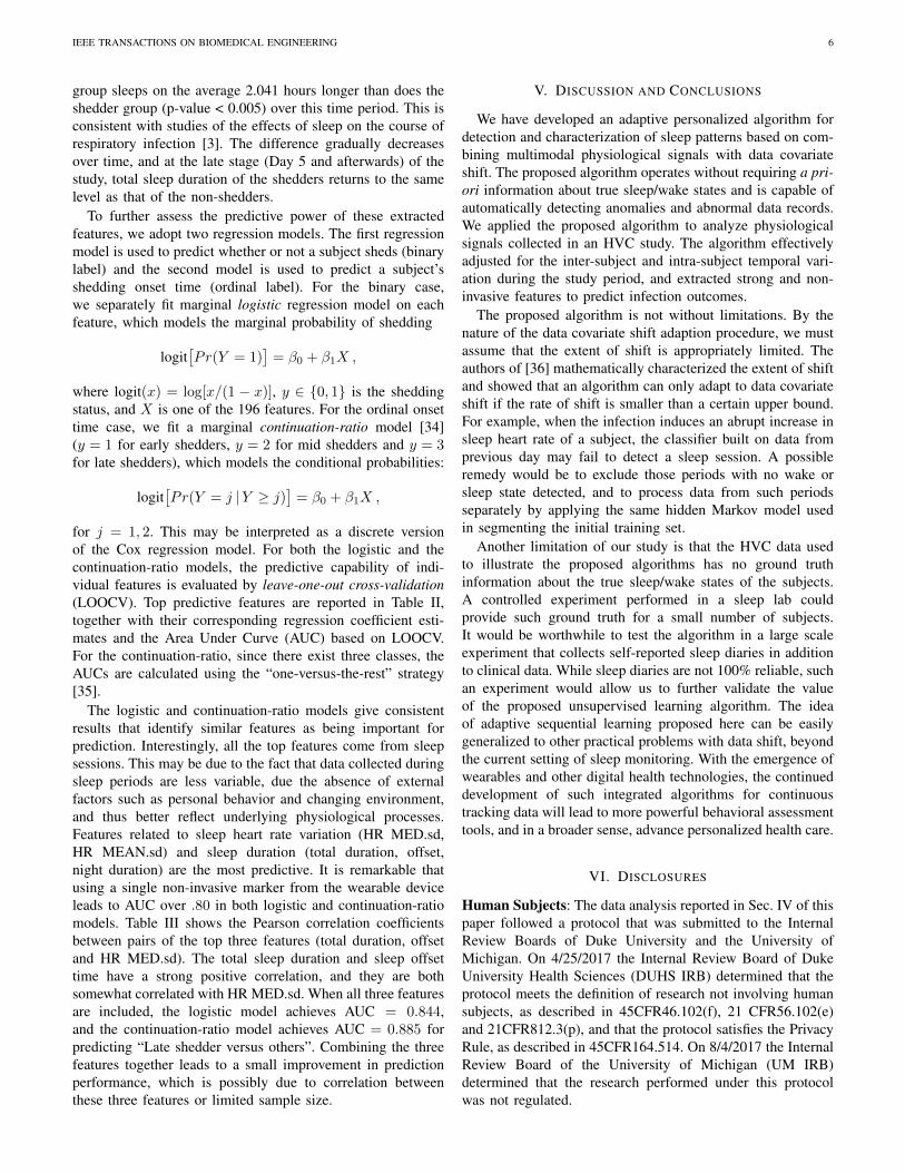
In this paper, we develop an unsupervised transfer learn-ing algorithm based on multivariate hidden Markov model(HMM) and Fisher’s linear discriminant analysis (LDA) toinfer the sleep/wake states of an individual under perturbedenvironments using multimodal signals collected by a portablesystem, such as a wearable device. The proposed algorithmdoes not require a priori information about true states fortraining, and adaptively adjusts to sleep pattern shift bysequentially re-training models with samples most relevantto the current time point. We illustrate an application of theproposed algorithm on tracking data collected by a wearablewristband in an HVC study. Through the detected sleep/wakesessions, we discovered several physiological features stronglypredictive to early-stage infection outcomes of clinical im-portance, including infection status and infection onset time.Figure 1a shows a general pipeline of processing and analyzingpersonal wearable data, consisting of an adaptive thresholdingmodule for anomaly filtering and a sequential learning module(Figure 1b) based on HMM and Fisher’s LDA.

The remainder of this paper is organized as follows: weintroduce data pre-processing steps in Section II. Section IIIpresents the proposed algorithm for sleep/wake detection indetail. Section IV contains an application of the proposedalgorithm to wearable data collected in an HVC study, withadditional results from statistical analyses of the detectedsleep/wake sessions. Finally, Section V contains some con-cluding remarks.

II. DATA PRE-PROCESSING

Our algorithm aims to detect sleep/wake sessions basedon multimodal physiological signals captured by a portablesystem, such as 3-axis acceleration, heart rate, and skintemperature. Wearable sensors often capture data at highfrequencies, and because of the fact that they are worn bysubjects in non-laboratory situations, the raw data collected

are often voluminous and noisy. We propose a pre-processingpipeline for the raw sensor data containing the following steps.

A. Segmentation and summarization

To mitigate the impact of occasional poor readings andreduce computational burden, we segment the whole timelineinto non-overlapping epochs of equal length. Three summarystatistics, namely, mean (MEAN), median (MED) and standarddeviation (SD), are extracted from each type of bio-signalwithin each epoch. For one epoch, if more than 90% ofthe designed capacity (sampling frequency × epoch lengthin seconds) is not observed, such as when the device waspowered-off, data from this epoch is marked as “not available(NA)". The resulting summary statistics from the three typesof signals are denoted by{

Xi,t, i = 1, . . . , n, t = t1, t2, . . . , tN},

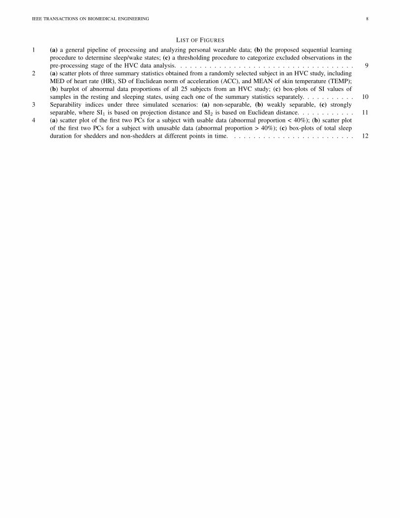
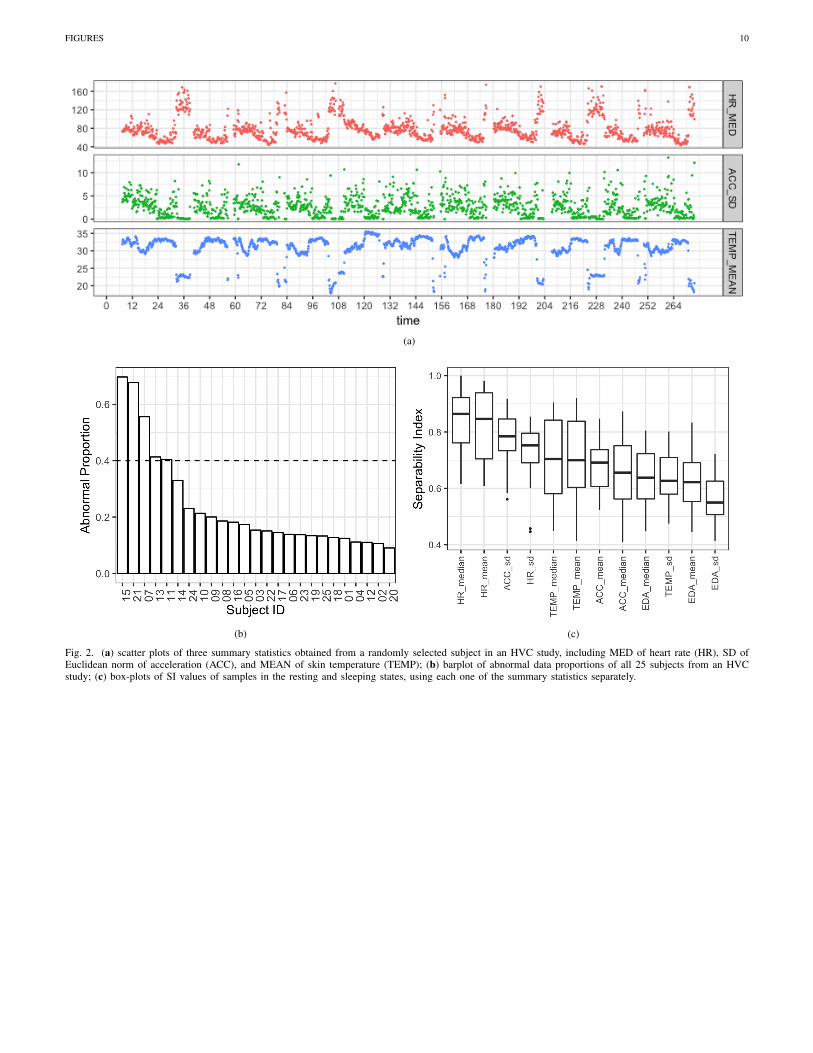
where t is the time stamp aligned to a certain origin witht1, t2, . . . , tN denoting respective starting times of each epoch,and Xi,t represents a 3×p-dimensional vector of the summarystatistics for subject i during an epoch starting at t with p beingthe number of signals available. As an example, Figure 2ashows scatter plots of three summary statistics obtained from arandomly selected subject in an HVC study, including MED ofheart rate (HR), SD of Euclidean norm of acceleration (ACC),and MEAN of skin temperature (TEMP).

B. Abnormal observations filtering

Summarization alone cannot handle abnormal readings thatoccur over an extended period of time. In the example shownin Figure 2a, it is clear that there exist abnormal values inthe summarized data, such as biologically impossible lowtemperature (e.g. < 20◦C) or extremely high heart rate (e.g.> 160bpm). This could be due to poor contact of sensors tothe subject or simply the case that the device was not wornduring the time period. These abnormal readings can seriouslycompromise the performance of our sleep detection algorithmintroduced in Section III, and therefore we propose an adaptivethresholding procedure using a subset of summary variablesXi,t = (X1i,t, . . . , XMi,t). The selected variables should havedistinctive distributions under normal and abnormal situations.For example, the mean temperature is usually much lower inabnormal cases, when the sensor measures ambient tempera-ture rather than body temperature. We then filter out data thatwith Xi,t /∈ Ci, where Ci is a joint feasible region determinedby a sequence of cutoff values {ci1, . . . , ciM} for Xi,t.

The subject dependent cutoff values are obtained by sep-arately performing k-means clustering on each variable inXi,t, and partitioning samples into three clusters, corre-sponding to three states: sleep, wake and abnormal. Let{Sim1, Sim2, Sim3} be the resulting clusters with centers(centroids) {µim1, µim2, µim3} arranged in descending order.Consider again the example of mean temperature. The clusterSim3 having the smallest center value was observed to con-sist of abnormal samples. Occasionally, the variation withinabnormal samples is even larger than the difference betweensleep and wake state, in which case the middle cluster may


also contain abnormal samples. We identify these cases bycomparing the distances between Sim1, Sim2 and Sim2, Sim3.Specifically, the set of normal, i.e., non-abnormal, samplesSnorim based on mean temperature is determined as follows:

Snorim =

{Sim1 ∪ Sim2 if |µim2 − µim1| < |µim3 − µim2|,Sim1 o.w..

With the normal sets Snorim for m = 1, · · · ,M , the cutoff

values are then

cim =

{Q0.025({Xmi,t ∈ Snor

im }) if µi,nor > µi,abn,

Q0.975({Xmi,t ∈ Snorim }) o.w.,

where Qq(·) calculates the q−quantile of samples, and µi,nor,µi,abn are mean measurement values of the normal and abnor-mal set, respectively. To robustify our classification procedureswe used a quantile-thresholding rule to exclude samples nearthe boundary of the normal set. We found the 2.5% and97.5% quantiles to provide adequate robustness for our databut other threshold values may be selected at the discretionof the analyst. The feasible interval for Xmi,t is [cim,+∞) ifµi,nor > µi,abn and (−∞, cim] otherwise.

III. AN ADAPTIVE SLEEP DETECTION ALGORITHM

We propose an adaptive sequential learning algorithm toidentify sleep periods using multimodal bio-signals, whichaccounts for a potential sleep pattern shift due to perturbedenvironments. The proposed algorithm is applied to each sub-ject separately. Thus, for simplicity of notation, we suppressthe subscript i in the following discussion.

A. Initial training set based on hidden Markov model

We first establish an initial training set Sini ={(xt, yt), t = t1, . . . , tn0

}using a multivariate hidden

Markov model (HMM) [23], where xt is a subset of observedsummary statistics Xt, relevant to the circadian pattern, andyt is the latent label indicating sleep status (yt = 0 if wake;yt = 1 if sleep). The end point tn0 of the initial training set isselected as the time before potential perturbation on the sleeppattern, so that we can posit a multivariate HMM as follows:

xt | (ut = k) ∼ N(µk,Σk), k = 1, . . . ,K,

where the discrete latent variable ut follows a Markov processwith transition matrix AK×K . The variable ut is closelyrelated to, but not necessarily the same as, yt dependingon whether xt has multiple states during wake sessions. Infact, the sleep/wake label yt estimates are derived from theestimated latent variable ut. For example, the mean heart ratemay have two different states (resting and active) when thesubject is awake, in which case ut has three states, i.e., K = 3,with both the resting and active state corresponding to yt = 0.In the following discussion, we will focus on the derivedbinary label yt, since our primary goal is to detect sleep/wakesessions.

To select the optimal set of xt as well as optimal numberof states K for each subject, we suggest first specifying alist of possible model configurations, for example, a two-state

trivariate HMM using MEAN and SD of heart rate and SD ofacceleration. A series of HMMs are then fitted and evaluatedby the separability index (SI) proposed in (4) and the HMMmodel with the maximum SI from the pool of candidates isselected as the model for deciding sleep/wake states yt in theinitial training set.

B. Sequential learning with Fisher’s LDA

Due to potentially perturbed environments, the underlyingdistribution of xt | yt may not be stationary over time. Thus,the initial training set cannot be directly used to determine thesleep labels for subsequent epochs. We propose performingFisher’s LDA in a sequential fashion using the same summarystatistics as used in the chosen HMM, resulting in a dynamicclassifier that is capable of adjusting for covariate shift.Panel (b) in Figure 1 demonstrates this sequential learningprocedure and Algorithm 1 below summarizes the major stepsto implement it.

Fisher’s LDA is a powerful tool for dimension reduction andclassification [24]. It is motivated by the idea of finding theoptimal direction vector w, onto which the projected scoresof training samples have the largest “separability" betweenclasses. Let the training dataset be

{(xt, yt), t ∈ Ttrn

}and

let zt = wTxt denote the projected scores. The separabilityis measured by the following ratio of between-class variationand within-class variation:

J(w) =(z1· − z)2 + (z0· − z)2∑

t∈G1(zt − z1·)2 +

∑t∈G0

(zt − z0·)2, (1)

where Gk = {t : yt = k, t ∈ Ttr} for k = 0, 1 denote indicesof data from two classes, respectively, zk· =

∑t∈Gk

zt/|Gk|for k = 0, 1 are the class-specific mean scores and z is theoverall mean score. The optimal w that maximizes (1) is

w = S−1W (x1· − x0·), (2)

where xk· =∑

t∈Gkxt/|Gk| for k = 0, 1 and SW =∑

k=0,1

∑t∈Gk

(xt − xk·)(xt − xk·)T , known as the within-

class scatter matrix. Let σ2k =

∑t∈Gk

(zt − zk·)2/(|Gk| − 1)for k = 0, 1 be the class-specific sample variances. For a testsample xt′ , we build a classifier based on the projection vectorw from Fisher’s LDA and predict the label using the followingrule:

yt′ = 1

{(zt′ − z0·)2

σ20

− (zt′ − z1·)2

σ21

> log

(γσ21

σ20

)}, (3)

wherezt′ = wTxt′ and γ is a multiplicative factor for thethreshold with its value set to 1 by default in our HVC analysis.In other words, the label of a test sample depends on therelative distance of the sample to the class centroids weightedby dispersion. Assuming the conditional distribution xt | ytis multivariate normal for both classes, it is easy to show that(3) is equivalent to the Naive Bayes classifier [24] based onthe projected score z.

While the sleep pattern may gradually shift over time,we will assume that the change is negligible within a shortwindow. Therefore, we process and predict sleep labels in-crementally within batches of non-overlapping time windows


Algorithm 1 Sequential learning with adaptive-size sliding window1: current = tn0

. Start from the initial training set2: while current < tN do . Continue until all epochs are labeled3: for l in 1 to L do . Consider all window lengths4: procedure FISHER’S LDA(train = (current− dl, current], test = (current, current+ ∆t])5: w = S−1W (x1· − x0·)6: zt′ = wTxt′

7: yt′ = 1{

(zt′ − z0·)2/σ20 − (zt′ − z1·)2/σ2

1 > log(γ σ21/σ

20)}

8: SI(dl) = SI(train, test; dl) . Separability index for a given window lengths9: d0 = which.max(SI(dl)) . Select the optimal window lengths with maximum SI

10: yt′,opt = yt′ | d0 . Determine the labels using the optimal window11: current = current+ ∆t . Move on to the next test batch

of pre-specified length ∆t. This is similar to approaches usedin online learning [25], except that we use predicted labelsinstead of true labels, which are not available to us. To bemore specific, after establishing the initial training set, weperform the Fisher’s LDA using the same summary statisticsas used in the chosen HMM and predict sleep labels for epochscoming from the next test batch

{xt, tn0 < t ≤ tn0 +∆t, t ∈

{t1, · · · , tN}}

. The processed batch is then added to the poolof labeled samples so as to form an enlarged training datasetused to renew Fisher’s LDA classifier. The process continuessequentially until all epochs are labeled.

Inspired by methods for concept drift adaption in thesupervised online learning literature [26], [27], [28], [29], weincorporate a taper windowing mechanism which excludesoutdated training samples that are distant in time from thecurrent batch under investigation and no longer representative.To implement this mechanism we adopt a sliding-windowtechnique for performing Fisher’s LDA in which only the mostrecently labeled training samples are used. The length of thewindow has to be carefully determined to achieve a desirableperformance. Unlike the case of supervised online learning,with no information on true labels, it is infeasible to selectoptimal window length by maximizing prediction accuracy intest batches. Instead, the separability index (SI) [30], [31] ismaximized as a proxy for accuracy. Specifically, first specify aset of candidate window lengths

{d1, · · · , dL

}. Then, letting

tn denote the most recent epoch with sleep label, and creatingTtrn(dl) =

{t : tn − dl < t ≤ tn, t ∈ {t1, · · · , tN}

}for

l = 1, · · · , L and Ttst ={t : tn < t ≤ tn + ∆t, t ∈

{t1, · · · , tN}}

, we define the epochs in the candidate trainingdatasets and test batch, respectively. For a single window oflength dl, perform an initial pass of Fisher’s LDA with trainingsamples {(xt, yt), t ∈ Ttrn(dl)}. Let w(dl) be the optimaldirection vector given by (2). Then, predict labels with asecond pass, using the resulting Fisher’s LDA classifier onthe test batch, and calculate the following separability indexof the joint set of training and test samples:

SI(dl) =

∑t∈Ttrn(dl)∪Ttst{yt + y(t) + 1} MOD 2

|Ttrn(dl)|+ |Ttst|, (4)

where yt is the sleep label for epoch starting at t (predictedlabel if t ∈ Ttst), and y(t) is the (predicted) label of its nearestneighbor. In our method, nearest neighbors are determined by

the “ projection distance” defined, for samples from epoch tand t′, as follows:

h(t, t′) = |w(dl)T (xt − xt′)|. (5)

Among the candidate window sizes, the one maximizing thecriterion SI(dl) is used to derive Fisher’s LDA that predictsthe sleep labels of samples in the current test batch.

The sleep periods are often detected as bursts, often con-sisting of one or more continuous sessions interrupted byshort time periods. While such bursty behavior could bedirectly incorporated into an HMM model, e.g., a semi-Markovswitching process, we take a simpler approach and smooththese short interruptions by applying a median filter on theestimated sleep state yt sequence. The whole timeline isthen partitioned into consecutive continuous sleep and wakesessions. If there exists prior information on the minimalduration of sleep/wake sessions of interest, it can be usedto set a threshold for detected session length. For example,the deep sleep period, defined as Stage 3 & 4 of non-rapideye movement (NREM) period, usually starts 30 minutes aftersleep onset and lasts approximately 20 to 40 minutes in thefirst sleep cycle [32]. Hence, a 60-minute threshold can beapplied to include only sleep sessions with at least one deepsleep period.

C. Separability index

By definition (4), SI is the proportion of samples whichshare the same label with their nearest neighbors, and henceSI ∈ [0, 1]. Intuitively, when samples from two classes formtwo tight, well-separated clusters with little overlap, the nearestneighbor of one sample from, say, Class 0, will most likelybelong to Class 0 as well, which will result in a large SIvalue close to 1. In contrast, when samples from two classesfollow exactly the same distribution, i.e., completely non-separable, then the nearest neighbor of one sample will haveequal probability of being Class 0 or Class 1, and thus, the SIof these samples is close to 0.5. A large SI value implies strongseparability of classes, and is usually an indication of reliableprediction. SI also depends on the measure of distance usedto determine the nearest neighbors. The projection distancecaptures the difference among samples on the optimal directionw that is most relevant to distinguishing between the two


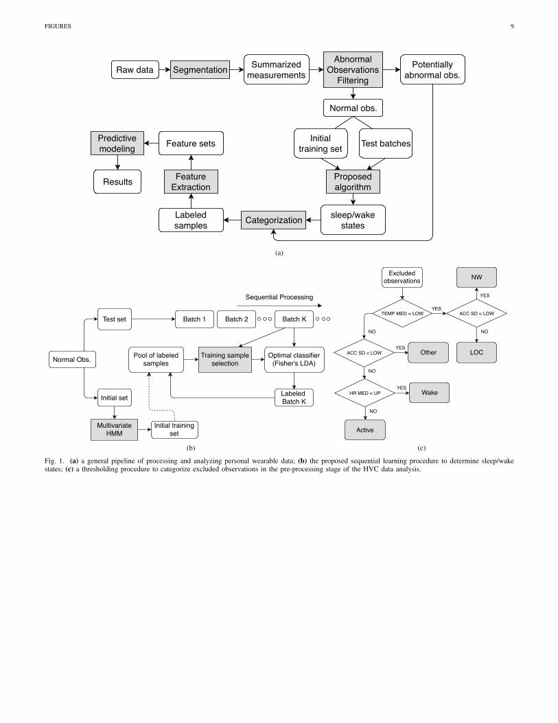
classes, and thus is better than Euclidean distance in regard tocharacterizing separability, as demonstrated by Figure 3.

Figure 3 illustrates three simulated cases with differentlevels of separability. Two variables (X1, X2) are generatedfrom BVN(µ1, µ2, 1, 1, 0). For samples in Class 0 (indicatedby red dots), µ1 = µ2 = 0, while for samples in Class 1(indicated by green triangles), we considered three settings:(1) µ1 = µ2 = 0; (2) µ1 = µ2 = 1.5; (3) µ1 = µ2 = 3, cor-responding to non-, weakly and strongly separable scenarios.SI values based on both projection distance and Euclideandistance are reported for each case. We observe that SI isindeed able to effectively characterize separability, and thatthe projection distance is preferred since it gives value closerto 0.5 in the non-separable case and value closer to 1 in thestrongly separable case.

IV. APPLICATION TO DATA FROM AN HVC STUDY

We applied the proposed algorithm to an anonymized ver-sion of a dataset collected from 25 participants enrolled in alongitudinal human viral challenge (HVC) study, which wasfunded by DARPA under the Prometheus program. In thishuman challenge study, some of the participants developeddisturbed sleep patterns shortly after infection by a pathogen(H3N2). Four channels of physiological signals, including 3-axis acceleration, heart rate, skin temperature and electroder-mal activity, were collected by a wrist-worn device, EmpaticaE4 (Empatica Inc. USA), over the time course of the study(11 days).

A. Adaptive sleep detection

The median (MED) of heart rate and skin temperaturewere used in the pre-processing stage for anomaly detection.Figure 2b shows the bar-plot of abnormal data proportions ofall subjects, and 5 of them were excluded from further analysesdue to high proportion of abnormal readings (> 40%).

To select proper candidate summary statistics for sleepdetection, we extracted data from a typical awake but restingperiod (21:00 - 22:00) and a sleeping period (03:00 - 04:00)for each subject. Separability indices of samples in the restingand sleeping states were then calculated marginally usingone summary statistic at a time. These indices were used asmeasures of the difference between these states. Figure 2cshows the box-plots of SI values for all summary statistics.We chose three summary statistics with high average SI values(> 0.7), namely, MED and SD of heart rate and SD ofacceleration, as candidates for xt. These summary statisticswere then used to identify sleep/wake sessions for the subjects.Note that MEAN and MED of heart rate are almost identical,so only MED is selected.

Based on the detected sleep/wake sessions, and using MEDof heart rate and skin temperature and SD of acceleration,we further categorized abnormal samples excluded in the pre-processing stage into the following states:• device not worn (NW): lower-than-normal TEMP MED

and lower-than-normal ACC SD;• lost of contact (LOC): lower-than-normal TEMP MED

and normal ACC SD;

• active: normal TEMP MED and higher-than-normal HRMED and ACC SD).

Here the normal ranges of these summary statistics are deter-mined by a well established rule of thumb [33] as follows:

LOW = Q0.25 − 1.5 ∗ (Q0.75 −Q0.25),

UP = Q0.75 + 1.5 ∗ (Q0.75 −Q0.25), (6)

where Q0.25 and Q0.75 are the 25% and 75% sample quantilesof the empirical distributions over detected wake sessions. Thiscategorization procedure is illustrated in Figure 1c.

We also performed principle component analysis (PCA)on the 3 × 4 summary statistics from all epochs for eachsubject separately. This analysis was used to confirm theeffectiveness of the proposed method in detecting abnormalsamples and sleep/wake sessions. Figures 4a and 4b showthe scatter plot of the first two principle components (PC)for a subject with usable data (abnormal proportion < 40%)and a subjects with unusable data (abnormal proportion >40%). For the subject with usable data, the data points formdistinct clusters consistent with the categories identified bythe proposed method. The subject with unusable data presentsa completely different pattern in its PCA components, withthe abnormal observations showing a systematic trend thatcorresponds to a device that is either malfunctioning, not wornproperly, or not worn.

B. Predictive modeling

Finally, we considered predicting clinical outcomes with the196 features extracted from the identified sleep/wake sessions.Each wake session is assigned to a day according to its onsettime, while a sleep session is assigned to its onset day ifthere exists a substantial wake period (> 5 hours) prior to thesession. Otherwise, it is assigned to the previous day. Table Isummarizes the physiological features derived from sleep andwake sessions for each day, where duration and onset/offsettimes are exclusive features for sleep sessions, while the othersare shared by sleep and wake sessions. The linear/quadraticcoefficients are obtained from running linear and quadraticregression models of each summary statistic computed overa time of day. All features related to standard deviation arelog-transformed.

The 20 subjects with usable data are classified accordingto the clinical outcome of accumulated viral shedding fromthe zeroth to the fifth day. Subjects in the first class are thosewho showed positive accumulated viral shedding, and they arecalled “shedders.” In this dichotomization, eight of 20 suchsubjects are shedders, while 12 others are “non-shedders”.In addition, using a three-level ordinal scale, subjects withpositive viral shedding within 48 hours after inoculation aredenoted “early shedders” (2 out of 20); those with positiveviral shedding between 48 hours and 72 hours are denoted“mid shedders” (6 out of 20), and others are denoted “lateshedders” (12 out of 20, identical to non-shedders).

Figure 4c shows box-plots of total sleep duration for shed-ders and non-shedders at different points in time. We observea clear difference between the two groups on Day 0, whichis the first 24 hours after viral inoculation. The non-shedder


group sleeps on the average 2.041 hours longer than does theshedder group (p-value < 0.005) over this time period. This isconsistent with studies of the effects of sleep on the course ofrespiratory infection [3]. The difference gradually decreasesover time, and at the late stage (Day 5 and afterwards) of thestudy, total sleep duration of the shedders returns to the samelevel as that of the non-shedders.

To further assess the predictive power of these extractedfeatures, we adopt two regression models. The first regressionmodel is used to predict whether or not a subject sheds (binarylabel) and the second model is used to predict a subject’sshedding onset time (ordinal label). For the binary case,we separately fit marginal logistic regression model on eachfeature, which models the marginal probability of shedding

logit[Pr(Y = 1)

]= β0 + β1X ,

where logit(x) = log[x/(1 − x)], y ∈ {0, 1} is the sheddingstatus, and X is one of the 196 features. For the ordinal onsettime case, we fit a marginal continuation-ratio model [34](y = 1 for early shedders, y = 2 for mid shedders and y = 3for late shedders), which models the conditional probabilities:

logit[Pr(Y = j |Y ≥ j)

]= β0 + β1X ,

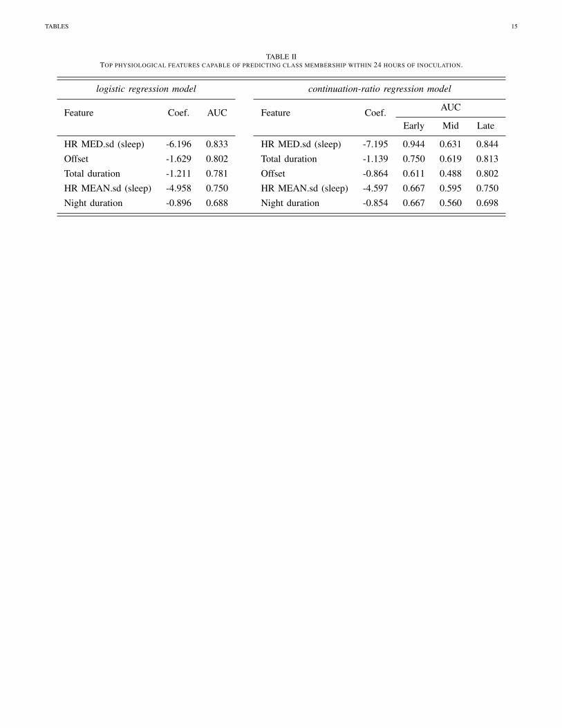
for j = 1, 2. This may be interpreted as a discrete versionof the Cox regression model. For both the logistic and thecontinuation-ratio models, the predictive capability of indi-vidual features is evaluated by leave-one-out cross-validation(LOOCV). Top predictive features are reported in Table II,together with their corresponding regression coefficient esti-mates and the Area Under Curve (AUC) based on LOOCV.For the continuation-ratio, since there exist three classes, theAUCs are calculated using the “one-versus-the-rest” strategy[35].

The logistic and continuation-ratio models give consistentresults that identify similar features as being important forprediction. Interestingly, all the top features come from sleepsessions. This may be due to the fact that data collected duringsleep periods are less variable, due the absence of externalfactors such as personal behavior and changing environment,and thus better reflect underlying physiological processes.Features related to sleep heart rate variation (HR MED.sd,HR MEAN.sd) and sleep duration (total duration, offset,night duration) are the most predictive. It is remarkable thatusing a single non-invasive marker from the wearable deviceleads to AUC over .80 in both logistic and continuation-ratiomodels. Table III shows the Pearson correlation coefficientsbetween pairs of the top three features (total duration, offsetand HR MED.sd). The total sleep duration and sleep offsettime have a strong positive correlation, and they are bothsomewhat correlated with HR MED.sd. When all three featuresare included, the logistic model achieves AUC = 0.844,and the continuation-ratio model achieves AUC = 0.885 forpredicting “Late shedder versus others”. Combining the threefeatures together leads to a small improvement in predictionperformance, which is possibly due to correlation betweenthese three features or limited sample size.

V. DISCUSSION AND CONCLUSIONS

We have developed an adaptive personalized algorithm fordetection and characterization of sleep patterns based on com-bining multimodal physiological signals with data covariateshift. The proposed algorithm operates without requiring a pri-ori information about true sleep/wake states and is capable ofautomatically detecting anomalies and abnormal data records.We applied the proposed algorithm to analyze physiologicalsignals collected in an HVC study. The algorithm effectivelyadjusted for the inter-subject and intra-subject temporal vari-ation during the study period, and extracted strong and non-invasive features to predict infection outcomes.

The proposed algorithm is not without limitations. By thenature of the data covariate shift adaption procedure, we mustassume that the extent of shift is appropriately limited. Theauthors of [36] mathematically characterized the extent of shiftand showed that an algorithm can only adapt to data covariateshift if the rate of shift is smaller than a certain upper bound.For example, when the infection induces an abrupt increase insleep heart rate of a subject, the classifier built on data fromprevious day may fail to detect a sleep session. A possibleremedy would be to exclude those periods with no wake orsleep state detected, and to process data from such periodsseparately by applying the same hidden Markov model usedin segmenting the initial training set.

Another limitation of our study is that the HVC data usedto illustrate the proposed algorithms has no ground truthinformation about the true sleep/wake states of the subjects.A controlled experiment performed in a sleep lab couldprovide such ground truth for a small number of subjects.It would be worthwhile to test the algorithm in a large scaleexperiment that collects self-reported sleep diaries in additionto clinical data. While sleep diaries are not 100% reliable, suchan experiment would allow us to further validate the valueof the proposed unsupervised learning algorithm. The ideaof adaptive sequential learning proposed here can be easilygeneralized to other practical problems with data shift, beyondthe current setting of sleep monitoring. With the emergence ofwearables and other digital health technologies, the continueddevelopment of such integrated algorithms for continuoustracking data will lead to more powerful behavioral assessmenttools, and in a broader sense, advance personalized health care.

VI. DISCLOSURES

Human Subjects: The data analysis reported in Sec. IV of thispaper followed a protocol that was submitted to the InternalReview Boards of Duke University and the University ofMichigan. On 4/25/2017 the Internal Review Board of DukeUniversity Health Sciences (DUHS IRB) determined that theprotocol meets the definition of research not involving humansubjects, as described in 45CFR46.102(f), 21 CFR56.102(e)and 21CFR812.3(p), and that the protocol satisfies the PrivacyRule, as described in 45CFR164.514. On 8/4/2017 the InternalReview Board of the University of Michigan (UM IRB)determined that the research performed under this protocolwas not regulated.


Conflict-of-interest: The authors have no conflicts of interestto disclose.

REFERENCES

[1] M. A. Miller, “The role of sleep and sleep disorders in the development,diagnosis, and management of neurocognitive disorders,” Frontiers inneurology, vol. 6, p. 224, 2015.

[2] M. R. Irwin, “Why sleep is important for health: a psychoneuroim-munology perspective,” Annual review of psychology, vol. 66, 2015.

[3] C. L. Drake, T. A. Roehrs, H. Royer, G. Koshorek, R. B. Turner, andT. Roth, “Effects of an experimentally induced rhinovirus cold on sleep,performance, and daytime alertness,” Physiology & behavior, vol. 71,no. 1-2, pp. 75–81, 2000.

[4] S. Cohen, W. J. Doyle, C. M. Alper, D. Janicki-Deverts, and R. B.Turner, “Sleep habits and susceptibility to the common cold,” Archivesof internal medicine, vol. 169, no. 1, pp. 62–67, 2009.

[5] K. A. Kaplan, J. Hirshman, B. Hernandez, M. L. Stefanick, A. R.Hoffman, S. Redline, S. Ancoli-Israel, K. Stone, L. Friedman, J. M.Zeitzer et al., “When a gold standard isnâAZt so golden: Lack ofprediction of subjective sleep quality from sleep polysomnography,”Biological psychology, vol. 123, pp. 37–46, 2017.

[6] J. Dunn, R. Runge, and M. Snyder, “Wearables and the medicalrevolution,” Personalized medicine, vol. 15, no. 5, pp. 429–448, 2018.

[7] A. Rechtschaffen and A. Kales, “A manual of standardized terminology,techniques and scoring system of sleep stages in human subjects,” BrainInformation Service, University of California, Los Angeles.

[8] A. Flexerand, G. Dorffner, P. Sykacekand, and I. Rezek, “An automatic,continuous and probabilistic sleep stager based on a hidden markovmodel,” Applied Artificial Intelligence, vol. 16, no. 3, pp. 199–207, 2002.

[9] A. Malhotra, M. Younes, S. T. Kuna, R. Benca, C. A. Kushida, J. Walsh,A. Hanlon, B. Staley, A. I. Pack, and G. W. Pien, “Performance of anautomated polysomnography scoring system versus computer-assistedmanual scoring,” Sleep, vol. 36, no. 4, pp. 573–582, 2013.

[10] D. Y. Kang, P. N. DeYoung, A. Malhotra, R. L. Owens, and T. P.Coleman, “A state space and density estimation framework for sleepstaging in obstructive sleep apnea,” IEEE Transactions on BiomedicalEngineering, vol. 65, no. 6, pp. 1201–1212, 2018.

[11] R. J. Cole, D. F. Kripke, W. Gruen, D. J. Mullaney, and J. C. Gillin,“Automatic sleep/wake identification from wrist activity,” Sleep, vol. 15,no. 5, pp. 461–469, 1992.

[12] M. L. Blood, R. L. Sack, D. C. Percy, and J. C. Pen, “A compari-son of sleep detection by wrist actigraphy, behavioral response, andpolysomnography,” Sleep, vol. 20, no. 6, pp. 388–395, 1997.

[13] J. Hedner, G. Pillar, S. D. Pittman, D. Zou, L. Grote, and D. P. White,“A novel adaptive wrist actigraphy algorithm for sleep-wake assessmentin sleep apnea patients,” Sleep, vol. 27, no. 8, pp. 1560–1566, 2004.

[14] M. Marino, Y. Li, M. N. Rueschman, J. W. Winkelman, J. Ellenbogen,J. M. Solet, H. Dulin, L. F. Berkman, and O. M. Buxton, “Measuringsleep: accuracy, sensitivity, and specificity of wrist actigraphy comparedto polysomnography,” Sleep, vol. 36, no. 11, pp. 1747–1755, 2013.

[15] A. Sadeh, P. J. Hauri, D. F. Kripke, and P. Lavie, “The role of actigraphyin the evaluation of sleep disorders,” Sleep, vol. 18, no. 4, pp. 288–302,1995.

[16] S. Ancoli-Israel, R. Cole, C. Alessi, M. Chambers, W. Moorcroft, andC. P. Pollak, “The role of actigraphy in the study of sleep and circadianrhythms,” Sleep, vol. 26, no. 3, pp. 342–392, 2003.

[17] A. T. Van De Water, A. Holmes, and D. A. Hurley, “Objectivemeasurements of sleep for non-laboratory settings as alternatives topolysomnography–a systematic review,” Journal of sleep research,vol. 20, no. 1pt2, pp. 183–200, 2011.

[18] D. F. Kripke, E. K. Hahn, A. P. Grizas, K. H. Wadiak, R. T. Loving, J. S.Poceta, F. F. Shadan, J. W. Cronin, and L. E. Kline, “Wrist actigraphicscoring for sleep laboratory patients: algorithm development,” Journalof sleep research, vol. 19, no. 4, pp. 612–619, 2010.

[19] W. Karlen, C. Mattiussi, and D. Floreano, “Improving actigraphsleep/wake classification with cardio-respiratory signals,” in Engineeringin Medicine and Biology Society, 2008. EMBS 2008. 30th AnnualInternational Conference of the IEEE. IEEE, 2008, pp. 5262–5265.

[20] S. Saeb, T. R. Cybulski, S. M. Schueller, K. P. Kording, and D. C. Mohr,“Scalable passive sleep monitoring using mobile phones: opportunitiesand obstacles,” Journal of medical Internet research, vol. 19, no. 4,2017.

[21] J. G. Moreno-Torres, T. Raeder, R. Alaiz-RodríGuez, N. V. Chawla, andF. Herrera, “A unifying view on dataset shift in classification,” PatternRecognition, vol. 45, no. 1, pp. 521–530, 2012.

[22] S. J. Pan, Q. Yang et al., “A survey on transfer learning,” IEEETransactions on knowledge and data engineering, vol. 22, no. 10, pp.1345–1359, 2010.

[23] I. Visser, M. Speekenbrink et al., “depmixs4: an r package for hiddenmarkov models,” Journal of Statistical Software, vol. 36, no. 7, pp. 1–21,2010.

[24] J. Friedman, T. Hastie, and R. Tibshirani, The elements of statisticallearning. Springer series in statistics New York, NY, 2001.

[25] S. Shalev-Shwartz et al., “Online learning and online convex optimiza-tion,” Foundations and Trends R© in Machine Learning, vol. 4, no. 2, pp.107–194, 2012.

[26] G. Widmer and M. Kubat, “Learning in the presence of concept drift andhidden contexts,” Machine learning, vol. 23, no. 1, pp. 69–101, 1996.

[27] R. Klinkenberg and T. Joachims, “Detecting concept drift with supportvector machines,” in Proceedings of the 17th International Conferenceon Machine Learning, 2000, pp. 487–494.

[28] J. Gama, I. Žliobaite, A. Bifet, M. Pechenizkiy, and A. Bouchachia, “Asurvey on concept drift adaptation,” ACM computing surveys, vol. 46,no. 4, p. 44, 2014.

[29] L. I. Kuncheva and I. Žliobaite, “On the window size for classificationin changing environments,” Intelligent Data Analysis, vol. 13, no. 6, pp.861–872, 2009.

[30] C. Thornton, “Separability is a learner’s best friend,” in 4th NeuralComputation and Psychology Workshop, London, 9–11 April 1997.Springer, 1998, pp. 40–46.

[31] J. Greene, “Feature subset selection using Thornton’s separability indexand its applicability to a number of sparse proximity-based classifiers,”in Proceedings of Annual Symposium of the Pattern Recognition Asso-ciation of South Africa, 2001.

[32] M. A. Carskadon, W. C. Dement et al., “Normal human sleep: anoverview,” Principles and practice of sleep medicine, vol. 4, pp. 13–23, 2005.

[33] J. W. Tukey, Exploratory data analysis. Addison-Wesley, Reading, MA,1977.

[34] A. Agresti, Analysis of ordinal categorical data. John Wiley & Sons,2010, vol. 656.

[35] C. M. Bishop, Pattern recognition and machine learning. springer,2006.

[36] D. P. Helmbold and P. M. Long, “Tracking drifting concepts byminimizing disagreements,” Machine learning, vol. 14, no. 1, pp. 27–45,1994.


LIST OF FIGURES

1 (a) a general pipeline of processing and analyzing personal wearable data; (b) the proposed sequential learningprocedure to determine sleep/wake states; (c) a thresholding procedure to categorize excluded observations in thepre-processing stage of the HVC data analysis. . . . . . . . . . . . . . . . . . . . . . . . . . . . . . . . . . . . . 9

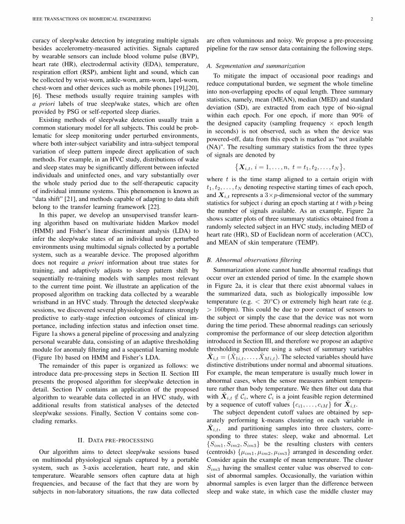
2 (a) scatter plots of three summary statistics obtained from a randomly selected subject in an HVC study, includingMED of heart rate (HR), SD of Euclidean norm of acceleration (ACC), and MEAN of skin temperature (TEMP);(b) barplot of abnormal data proportions of all 25 subjects from an HVC study; (c) box-plots of SI values ofsamples in the resting and sleeping states, using each one of the summary statistics separately. . . . . . . . . . . 10

3 Separability indices under three simulated scenarios: (a) non-separable, (b) weakly separable, (c) stronglyseparable, where SI1 is based on projection distance and SI2 is based on Euclidean distance. . . . . . . . . . . . 11

4 (a) scatter plot of the first two PCs for a subject with usable data (abnormal proportion < 40%); (b) scatter plotof the first two PCs for a subject with unusable data (abnormal proportion > 40%); (c) box-plots of total sleepduration for shedders and non-shedders at different points in time. . . . . . . . . . . . . . . . . . . . . . . . . . 12

FIGURES 9

Raw data Summarizedmeasurements

Potentiallyabnormal obs.

Normal obs.

SegmentationAbnormal

ObservationsFiltering

Initialtraining set Test batches

Proposedalgorithm

sleep/wakestatesCategorizationLabeled

samples

Feature sets

Results FeatureExtraction

Predictivemodeling

(a)

Normal Obs.

Initial set

Test set

MultivariateHMM

Initial trainingset

Batch 1 Batch 2 Batch K

Training sampleselection

Pool of labeledsamples

Optimal classifier (Fisher's LDA)

Labeled Batch K

Sequential Processing

(b)

Excludedobservations

TEMP MED < LOW ACC SD < LOWYES

NW

YES

LOC

NO

ACC SD < LOW

NO

HR MED < UP Wake

Active

Other

YES

YES

NO

NO

(c)

Fig. 1. (a) a general pipeline of processing and analyzing personal wearable data; (b) the proposed sequential learning procedure to determine sleep/wakestates; (c) a thresholding procedure to categorize excluded observations in the pre-processing stage of the HVC data analysis.

FIGURES 10

(a)

(b) (c)

Fig. 2. (a) scatter plots of three summary statistics obtained from a randomly selected subject in an HVC study, including MED of heart rate (HR), SD ofEuclidean norm of acceleration (ACC), and MEAN of skin temperature (TEMP); (b) barplot of abnormal data proportions of all 25 subjects from an HVCstudy; (c) box-plots of SI values of samples in the resting and sleeping states, using each one of the summary statistics separately.

FIGURES 11

(a) SI1 = 0.470, SI2 = 0.605 (b) SI1 = 0.750, SI2 = 0.785 (c) SI1 = 1.000, SI2 = 0.990

Fig. 3. Separability indices under three simulated scenarios: (a) non-separable, (b) weakly separable, (c) strongly separable, where SI1 is based on projectiondistance and SI2 is based on Euclidean distance.

FIGURES 12

(a) (b)

(c)

Fig. 4. (a) scatter plot of the first two PCs for a subject with usable data (abnormal proportion < 40%); (b) scatter plot of the first two PCs for a subjectwith unusable data (abnormal proportion > 40%); (c) box-plots of total sleep duration for shedders and non-shedders at different points in time.

FIGURES 13

LIST OF TABLES

I Features (196 in total) extracted from sleep (100) and wake (96) sessions for each day from 20 subjects in anHVC study. . . . . . . . . . . . . . . . . . . . . . . . . . . . . . . . . . . . . . . . . . . . . . . . . . . . . . . . 14

II Top physiological features capable of predicting class membership within 24 hours of inoculation. . . . . . . . . 15III Pairwise Pearson correlations among top three features. . . . . . . . . . . . . . . . . . . . . . . . . . . . . . . . 16

TABLES 14

TABLE IFEATURES (196 IN TOTAL) EXTRACTED FROM SLEEP (100) AND WAKE (96) SESSIONS FOR EACH DAY FROM 20 SUBJECTS IN AN HVC STUDY.

Name Number Description

Duration 2 total sleep, night sleepOnset/offset 2 night sleep onlyHR summary 9×2 3 (mean, median, s.d.) × 3 (mean, median, s.d. within session) × 2 (sleep, wake)HR linear coef. 6×2 3 (mean, median, s.d.) × 2 (coef.0, coef.1) × 2 (sleep, wake)HR quadratic coef. 9×2 3 (mean, median, s.d.) × 3 (coef.0, coef.1, coef.2) × 2 (sleep, wake)TEMP 24×2 same as HRACC 24×2 same as HREDA 24×2 same as HR

TABLES 15

TABLE IITOP PHYSIOLOGICAL FEATURES CAPABLE OF PREDICTING CLASS MEMBERSHIP WITHIN 24 HOURS OF INOCULATION.

logistic regression model continuation-ratio regression model

Feature Coef. AUC Feature Coef. AUC

Early Mid Late

HR MED.sd (sleep) -6.196 0.833 HR MED.sd (sleep) -7.195 0.944 0.631 0.844Offset -1.629 0.802 Total duration -1.139 0.750 0.619 0.813Total duration -1.211 0.781 Offset -0.864 0.611 0.488 0.802HR MEAN.sd (sleep) -4.958 0.750 HR MEAN.sd (sleep) -4.597 0.667 0.595 0.750Night duration -0.896 0.688 Night duration -0.854 0.667 0.560 0.698

TABLES 16

TABLE IIIPAIRWISE PEARSON CORRELATIONS AMONG TOP THREE FEATURES.

Total duration Offset HR MED.sd

Total duration 1 0.778 0.434Offset 1 0.485HR MED.sd 1

ieee transactions on biomedical engineering 1 an

Documents