Identifying preferences for public transport investments under a constrained budget

David Hensher, Chinh Ho, and Corinne MulleyInstitute of Transport and Logistics Studies

TRB 94th Annual Meeting January 11 – 15, 2015 Washington, D.C.

Outline

› Introduction

› Public preference survey

› Model

› Results

› Summary and policy relevance

2

Introduction

› Urban areas face increasing demand for new public transport investments.› Budgets are often constrained.› Public preference is important to understand from the community

perspective- How government should spend money and gain voter support, and

- To answer questions like

- How the public would temper their preference for a new modern light rail system if its geographical scope were to be limited by budget considerations?

- How society would view a bus based system giving greater network coverage for the same budget outlay as a proposed modern rail-based system?

3

Drivers of Public Preferences for PT

› Relevant factors associated with modal image, service quality and voting preferences were shortlisted through a best–worst experiment (phase I).

› 20 key drivers are classified into four groups:- Investment (construction time, route length, population coverage, ROW, maintenance cost)

- Service (capacity, peak and off-peak frequency, travel time vs car, fare vs car-related costs)

- Design (Ticketing, Transfer, boarding, safety and security)

- General characteristics (assured period of operation, risk of closing down after this assured period, level of attracting business around stations/stops, % car users switch to the system, environmental friendliness).

› The list of drivers is not complete for some respondents while surplus for others. The survey instrument accounts for this.

4

Choice Experiment – Unlabelled

5

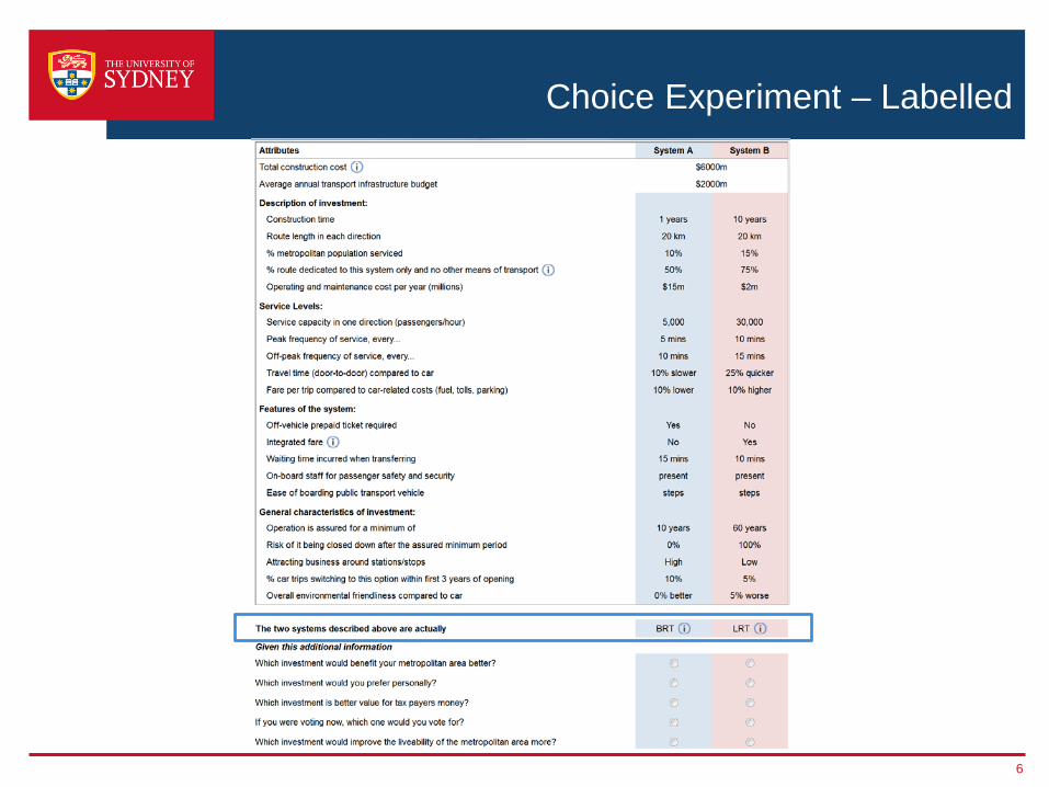
Choice Experiment – Labelled

6

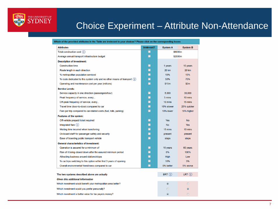
Choice Experiment – Attribute Non-Attendance

7

Choice Experiment – Not included Attributes

8

The Survey

› Online survey with panels from PureProfile and SSI› A pilot survey design used D-error measure and distributed to 200

respondents (100 samples from each panel)› Model estimated on the pilot sample to obtain priors for the main survey› Stated Choice Experiment redesigned and distributed to 400 PureProfile

respondents› Model re-estimated on 600 samples to obtain more accurate priors› SC survey redesigned and distributed to 400 SSI respondents› Respondents were sought in all Australian capital cities with population-

based quotas applied for each phase› A total sample of 1,018 respondents was obtained (18 surplus), giving

2,036 observations for final model estimation

9

The Sample

City Actual TargetSydney 271 270Melbourne 241 240Canberra 100 100Brisbane 201 200Adelaide 80 50Perth 70 50Darwin 21 50Hobart 34 50Total 1,018 1,010

Socio-economic profile Mean (std.dev)Age (years) 43.84 (15.5)

Proportion full time employed 0.41

Proportion part time employed 0.19

Proportion students 0.17

Working hours per week 20.75 (16.99)

Number of adults in household 2.11 (0.89)

Number of children in household 0.66 (1.03)

Personal income in $1000 62.47 (40.47)

Number of cars in household 1.66 (0.98)

Member of PT association (%) 9

Member of env. association (%) 6

10

The Model

› Mixed logit models with heteroscedastic conditioning and error components (HMLEC) with vs. without attributes non-attendance (ANA)

› Utility that the qth voter derives from alternative j:

› Probability that person qth votes for PT system j in choice situation c:

Budget Modal(BRT=1)

1δ M(1 )[ (0 , ) ]

jjqcq j kjq kjqq

Kjq ANAkjqq k jqU B X

=γ ε+= + α + β +∑

Parameter estimate under ANA

{ }{ }

1

1

2

1

2exp (1 ) (0 , ) ( )

ex

exp

exp (1 ) (0 , ) )p(

j kjq kjq cq

qc

j kjq kjq cq

Kq cq iq jq ANAkjq q jq jqk

jqc JK

q cq iq jq ANAkjq q j

j

j q jqkj

B M X B MP

B M X B M

=

==

+ δ + γ α + β + λ + η θ

= + δ + γ α + β + λ + η θ

∑

∑ ∑

11

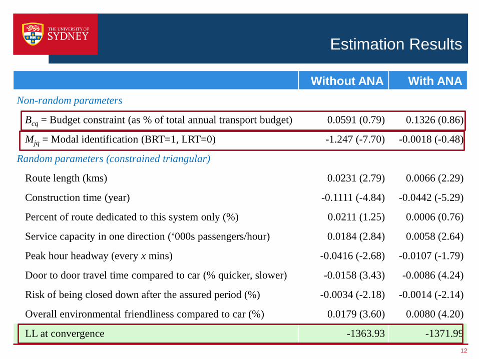
Estimation Results

Without ANA With ANANon-random parameters

Bcq = Budget constraint (as % of total annual transport budget) 0.0591 (0.79) 0.1326 (0.86)

Mjq = Modal identification (BRT=1, LRT=0) -1.247 (-7.70) -0.0018 (-0.48)

Random parameters (constrained triangular)

Route length (kms) 0.0231 (2.79) 0.0066 (2.29)

Construction time (year) -0.1111 (-4.84) -0.0442 (-5.29)

Percent of route dedicated to this system only (%) 0.0211 (1.25) 0.0006 (0.76)

Service capacity in one direction (‘000s passengers/hour) 0.0184 (2.84) 0.0058 (2.64)

Peak hour headway (every x mins) -0.0416 (-2.68) -0.0107 (-1.79)

Door to door travel time compared to car (% quicker, slower) -0.0158 (3.43) -0.0086 (4.24)

Risk of being closed down after the assured period (%) -0.0034 (-2.18) -0.0014 (-2.14)

Overall environmental friendliness compared to car (%) 0.0179 (3.60) 0.0080 (4.20)

LL at convergence -1363.93 -1371.9912

Utility Profiles

› Using fully compensatory model (w/o ANA)

. 57

1. 13

1. 70

2. 26

2. 83

. 00-. 250 . 000 . 250 . 500 . 750 1. 000 1. 250-. 500

ULRT UBRT

Dens

ity

. 26

. 52

. 78

1. 04

1. 30

. 00-2 -1 0 1 2 3-3

UTOTU UTOTLDe

nsity

BRT vs. LRT Modal labelled vs. Unlabelled

13

Marginal Rate of Substitution (MRS)

con_time (10 years)

ROW (%)

Capacity (1k pax/hour)

Peakfreq (mins)

TrvlTime (% quicker vs car)

Riskclose (%)

EnvFriendly (%)-1.0

0.0

1.0

2.0

3.0

4.0

5.0

Aver

age

WTP

±st

d de

v

Willingness to forgo 1km route length in return for other factors

BRT LRT BRT=LRT

14

Conclusions

› Under fully compensatory assumptions, it would seem that, however appealing the quality of service attributes, LRT is still preferred to BRT

› Once what really matters to each individual is narrowed down, LRT is no longer unambiguously preferred to BRT

› Budget constraint is of little interest to the community even if such a constraint has implications for how much of the new infrastructure can be built

› An ongoing challenge to identify ways to inform the population at large about the relative merits of bus-based public transport infrastructure solutions when budgets are constrained

15

Identifying preferences for public transport investments under a constrained budget

David Hensher, Chinh Ho, and Corinne MulleyInstitute of Transport and Logistics Studies

TRB 94th Annual Meeting January 11 – 15, 2015 Washington, D.C.

Resident Preference Model (Fixed Route Length)

› Identifying gains in voter support for BRT in the presence of LRT

BRT costs half LRT to build

BRT costs 75% LRT to build

BRT serves 50% more people

BRT has no negative prejudice

ROW: BRT 80%, LRT 20%

Voters are not familiar with BRT

BRT costs half LRT to build

Voters are familiar with BRT

BRT serves 50% more people

-4% -2% 0% 2% 4% 6% 8% 10% 12% 14%

Change to support for BRT

17