Identifying Multimodal, Non-Gaussian Parameter Distributions in

Groundwater Transport Modeling

Ming Ye (mye@fsu.edu) and Xiaoqing Shi (xshi@fsu.edu) Department of Scientific Computing, Florida State University

Gary Curtis: U.S. Geological Survey, Menlo ParkJichUn Wu: Department of Hydrosciences, Nanjing University, China

This research is supported in part by DOE SBR Grant: DE-SC0002687

NSF-EAR Grant: 0911074ORAU/ORNL High Performance Computing (HPC) Program

Uncertainty Quantification• “In a typical application of the statistical

paradigm, there's some quantity Δ about which I'm at least partially uncertain,

• and I wish to quantify my uncertainty about Δ, for the purpose of – sharing this information with other people (inference)

or – helping myself or others to make a choice in the face

of this uncertainty (decision-making).• Uncertainty quantification is usually based on a

probability model M, which relates Δ to known quantities (such as data values D).”

Model Uncertainty: why it matters and what to do about it (Draper)

Mathematical Formulation• Given a model M• Quantity of interest, Δdue to parametric uncertainty of the model• Predictions of Δ given observation D,

,p M D ,E M D ,Var M D0.10

0.08

0.06

0.04

0.02

0.00

p(

)

806040200 = Peak Dose (mrem/yr)

Reg

ulat

ory

Crit

erio

nor and

Meyer et al., 2007

Pathways of Groundwater Contamination

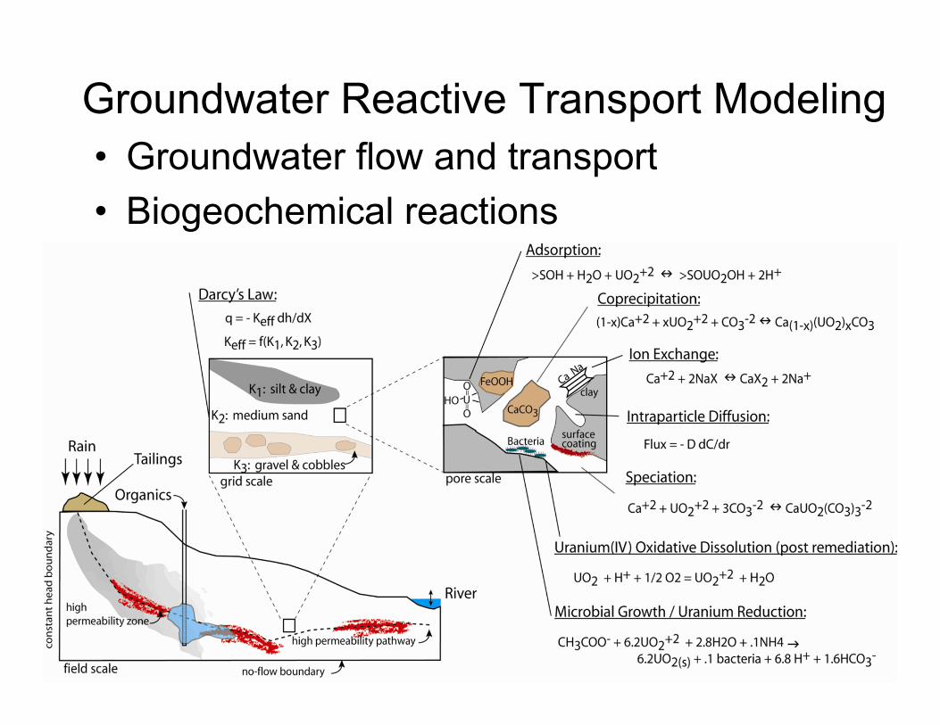
Groundwater Reactive Transport Modeling• Groundwater flow and transport• Biogeochemical reactions

Challenges in Uncertainty Quantification for Reactive Transport Modeling

• Groundwater reactive transport models are nonlinear with respect to its parameters due to nonlinear reaction equations and coupling of reactions and processes.

• The nonlinearity always leads to complex response surfaces of objective functions (e.g., least square or likelihood).

• As a result, probability distributions for model parameters may be non-Gaussian and have multiple modes, which questions the accuracy of the methods that assume (explicitly or implicitly) normal or lognormal distributions for parameters of reactive transport models.

Uranium Mill Tailing at Naturita, CO

• NATURITA MILL AND DISPOSAL SITE$86.3 million Cost of cleanup The Vanadium Corp. of America began operating the mill in 1939. The mill processed 704,000 tons of uranium ore for the Manhattan Project from 1942 to 1958. In the late 1970s, a private corporation bought the tailings pile and moved it to another site called Hecla/Durita to extract additional uranium and vanadium.

• Left behind: At and around the original mill, 138 acres were contaminated. Groundwater beneath the site was contaminated.

• The fix: From 1993 to 1997, DOE removed 800,000 yards of contaminated material and put it in a disposal site near Uravan. Contamination was left in place on 22 acres. More than one acre was left because the radiation levels were so high that workers would have been at risk.

http://www.denverpost.com/news/ci_15996355

Toxic legacy of uranium haunts proposed Colorado mill, By Nancy Lofholm, The Denver Post, 9/5/2010

Column ExperimentsColumn experiment (0.1m scale)

Kohler et al. (1996) studied U(VI) transport in laboratory columns packed with purified quartz powder.

Seven column experiments were conducted with different pH values and variable U(VI), F- and pH buffer concentrations.

The experiments were simulated with reactive transport modeling that combined surface complexation with aqueous speciation.

Surface Complexation Model (SCM)

• SjOH represents a surface hydroxyl functional groupand the subscript j denotes the type, each with a different binding affinity and surface site density

• Each SCM model contains the following adjustable parameters: surface complexation formation constant, K fraction (f) of the total surface site density for each site

type

2j 2 2 j 2S OH+UO +H O S OUO OH+2H

Model Parameters and Global Sensitivity Analysis

• The model has four parameters: – Three formation constants: logK1, logK2, and logK3– The fraction of the strong site: logSite

• The two most sensitive parameters: logK1 and logSite

0 2x103 4x103 6x103 8x103

Mean

2.0x103

4.0x103

6.0x103

8.0x103

104

1.2x104

logK1

logSite

logK3

logK2

Model C4 MOAT Analysis

2+ +1 2 2 1 2S OH+UO +H O=S OUO OH+2H

2+ +2 2 2 2 2S OH+UO +H O=S OUO OH+2H

2+ +2 2 2 2S OH+UO =S OUO +H

Weak Site:

Strong Site:

Model Calibration• The model is calibrated

against three experiments(Experiments 1, 2, and 8).

• The calibrated parametersgive satisfactory simulations.

• The rising limb is controlled by logK1 of the weak site and the declining limb by logK2 and logK3 of the strong site.

0 4 8 12 16 20Pore Volumes

0.2

0.4

0.6

0.8

1

Experiment 1SimulationObservation

0 2 4 6 8 10Pore Volumes

0.2

0.4

0.6

0.8

1

Experiment 2SimulationObservation

0 4 8 12 16Pore Volumes

0

0.2

0.4

0.6

0.8

1

Experiment 8SimulationObservation

Uncertainty Quantification

• When calculating the linear confidence interval, model parameters are assumed to be Gaussian.

• When calculating the nonlinear confidence interval, model parameters are assumed to have a single mode (not necessarily Gaussian).

• The intervals are too narrow, indicating that parameter uncertainty is underestimated.

C/C

0

• Use the calibrated model to predict data of another experiment (Expt 5) not used for the calibration.

• Predictive uncertainty is quantified using linear and nonlinear confidence interval.

Response Surface of Least-square Objective Functions

• Obtained using brute-force Monte Carlo with 120,000 simulations.• Response surface has multiple minima.• Global optimization is needed.• Parameter distributions are likely non-Gaussian and have multiple modes.

logK1 and logSite. logK1, logSite, and logK2.

• Parameter distribution with two modes

• Samples from the two modes

• Model simulations with two clusters: one is closer to observations than the other.

• Two minima exhibits, one global and the other local.

Simple Monte Carlo Simulations• Brute-force simulations, no numerical tricks.• Histograms of the four parameters indicate that the parameters

distributions are non-Gaussian and have multiple modes.

-8 -7.6 -7.2 -6.8 -6.4 -6 -5.6 -5.2 -4.8 -4.4 -4logK1

0

0.1

0.2

0.3

0.4

-3.4 -3.2 -3 -2.8 -2.6 -2.4 -2.2 -2 -1.8 -1.6 -1.4 -1.2 -1 -0.8 -0.6logSite

0

0.02

0.04

0.06

-4.8 -4.4 -4 -3.6 -3.2 -2.8 -2.4 -2 -1.6 -1.2logK2

0

0.01

0.02

0.03

0.04

0.05

0 0.2 0.4 0.6 0.8 1 1.2 1.4 1.6 1.8 2logK3

0

0.01

0.02

0.03

0.04

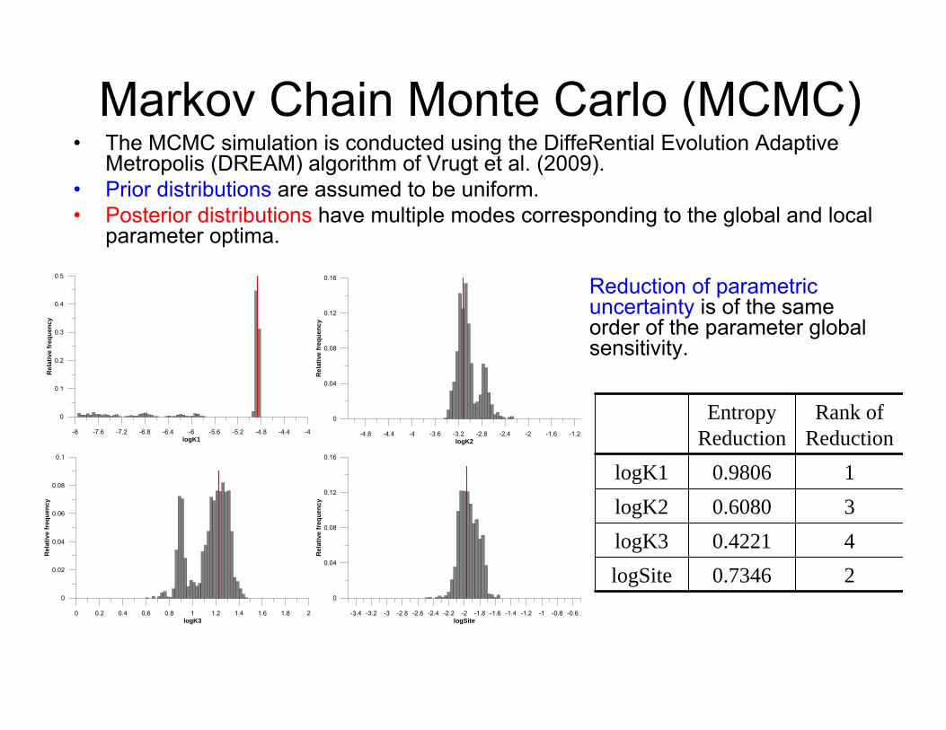
Markov Chain Monte Carlo (MCMC)• The MCMC simulation is conducted using the DiffeRential Evolution Adaptive

Metropolis (DREAM) algorithm of Vrugt et al. (2009). • Prior distributions are assumed to be uniform.• Posterior distributions have multiple modes corresponding to the global and local

parameter optima.

-8 -7.6 -7.2 -6.8 -6.4 -6 -5.6 -5.2 -4.8 -4.4 -4logK1

0

0.1

0.2

0.3

0.4

0.5

Rel

ativ

e fr

eque

ncy

-3.4 -3.2 -3 -2.8 -2.6 -2.4 -2.2 -2 -1.8 -1.6 -1.4 -1.2 -1 -0.8 -0.6logSite

0

0.04

0.08

0.12

0.16

Rel

ativ

e fr

eque

ncy

-4.8 -4.4 -4 -3.6 -3.2 -2.8 -2.4 -2 -1.6 -1.2logK2

0

0.04

0.08

0.12

0.16

Rel

ativ

e fr

eque

ncy

0 0.2 0.4 0.6 0.8 1 1.2 1.4 1.6 1.8 2logK3

0

0.02

0.04

0.06

0.08

0.1

Rel

ativ

e fr

eque

ncy

20.7346logSite40.4221logK330.6080logK210.9806logK1

Rank of Reduction

Entropy Reduction

Reduction of parametric uncertainty is of the same order of the parameter global sensitivity.

Uncertainty Quantification

• Calculating the credible interval does not make any assumptions on parameter distributions.

• The nonlinear credible interval is superior because of its larger coverage especially the peak of the breakthrough curve.

• Calculating the credible interval is computationally expensive, requiring thousands of model executions.

C/C

0

• Linear/nonlinear confidence intervals: Regression methods

• Nonlinear credible intervals: Bayesian methods.

Conclusions• Due to model nonlinearity, the response surface

of the least-square objective function is complex with heterogeneous mixture local minima and maxima of the objective function.

• This leads to non-Gaussian distributions of model parameters with multiple modes.

• For such parameter distributions, the conventional regression methods cannot accurately quantify parametric uncertainty.

• MCMC methods are effective and efficient for accurately quantifying predictive uncertainty in reactive transport modeling.