Ideal Polymer Chain.

Ideal Polymer Chain.Ideal chain is a chain in which the links do not interact if they are not close long the chain. In other words, the so-called volumeinteractions, i.e. interactions between distant links which come closeto each other due to the chain flexibility, are neglected.Polymer chains behave as ideal ones at the so-called Θ-conditions,(we will discuss this issue in more detail in one of the nextlectures).Consider first a freely-jointed chain of N segments of length l:

From the symmetry considerations, it is obvious that the mean end-to-end distance of the chain R equals 0. The size of the coil istherefore characterized by

→

Freely-Jointed Chain.

2

1 1 1 1

n n n n

i j i ji j i j

R u u u u= = = =

= = ∑ ∑ ∑∑

22

1 1 1 , 1,

n n n n

i j i i ji j i i j

i j

R u u u u u= = = =

≠

= = +∑∑ ∑ ∑

but for the freely-jointed chain 0i ju u =

for ,i j≠ and therefore

1i=

22 2 ,n

iR u Nl Ll L Nl= = = =∑

, where L is the contour length of the chain

2 1/ 2 ,R R N l R L=

Freely-Jointed Chain.

We see that:

- the conformation of the ideal chain is far from rectilinear;

- the ideal chain forms an entangled coil;

- the trajectory of the chain is equivalent to the trajectory of a Brownian particle.

2 1/ 2 ,R R N l R L=

Chain with a Fixed Valency Angle.

The aforementioned result for the typical coil size R ~ N , is valid for an ideal chain with any flexibility mechanism.Indeed, consider for example the model with fixed valency angleγ between the segments of length b (assume for simplicity that u(ϕ) = 0):

1/2

ϕγ

C C

C As before22

1 1 1 , 1,,

n n n n

i j i i ji j i i j

i j

R u u u u u= = = =

≠

= = +∑∑ ∑ ∑

2 2iu b=

, but now 0i ju u ≠

Instead of that we have:

2 2 2

, 1cos

n

iji ji j

R Nb b θ=

≠

= + ∑ , where θ is an angle between ith and jth segments.

ij

Chain with a Fixed Valency Angle.

γii+1

γii+1 i+2

, 1cos cosi iθ γ+ =

2, 2cos cosi iθ γ+ =

Continuing in the same way, we get ,cos coski i kθ γ+ = , and thus

2 2 2cos 1 cos21 cos 1 cos

Nb Nb Nbγ γγ γ

+≈ + =

− −

2 2 2 2 2,

1 1 1 12 cos 2 cos

N N i N N ik

i i ki k i k

R Nb b Nb bθ γ− −

+= = = =

= + = + ≈∑∑ ∑∑

(where k = j - i)

Chain with a Fixed Valency Angle.

The final result is, therefore:

Thus, within the model with a fixed valency angle we once again get an entangled coil: the typical size of the coil is once again proportional to the square root of the contour length of the chain. This result is a universal feature of the ideal chains regardless ofthe particular flexibility model.

For the value of R is larger than for the freely-jointed chain, while for it is smaller.

o90γ <o90γ >

2 1/ 2 1 cos1 cos

R R N b γγ

+=

−

Persistent Length of a Polymer Chain.

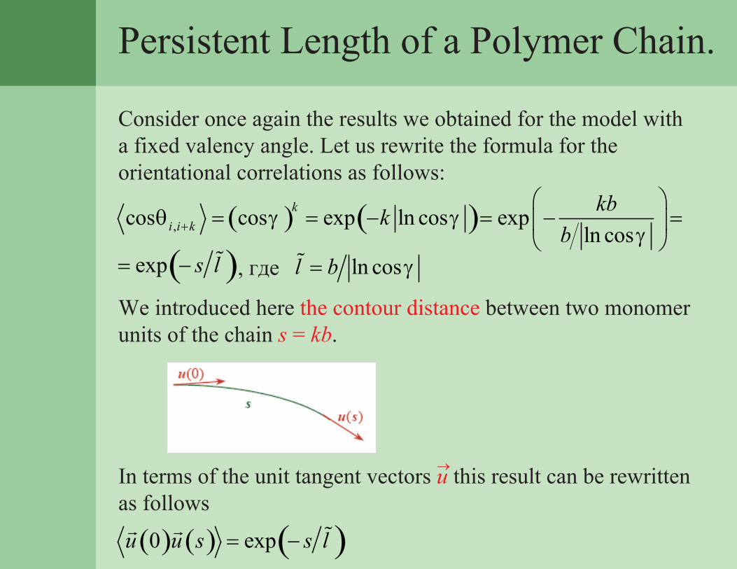
Consider once again the results we obtained for the model with a fixed valency angle. Let us rewrite the formula for the orientational correlations as follows:

( ) ( ),cos cos exp ln cos expln cos

ki i k

kbkb

θ γ γγ+

= = − = − =

( )exp s l= − , где ln cosl b γ=

We introduced here the contour distance between two monomerunits of the chain s = kb.

( ) ( ) ( )0 expu u s s l= −

In terms of the unit tangent vectors u this result can be rewritten as follows

→

Persistent Length of a Polymer Chain.

( ) ( ) ( )0 expu u s s l= −

We derived the formula within a modelwith a fixed valency angle. It is, however universal, i.e. validfor any model of polymer flexibility: orientational correlations decay exponentially along the chain.

For s << l the chain stays almost rectilinear, while at s >> l the memory about the chain orientation is completely lost.Therefore, one can divide an ideal chain into segments of lengthl and assume them to be rectilinear and independent from each other. Thus,

~

~ ~

2 2LR R l Lll

=

We get once again the same result: the size of the coil R is proportional to the square root of the chain length L.

~The characteristic length of this decay l is called a persistent length of the chain.

Kuhn Segment of a Polymer Chain.

We know now that for idea chain 2R LThe Kuhn segment length l of a chain is defined as

2l R L= (for large L)

(i.e., the equality is valid by definition)2R Ll=

Both l and l are used in actual practice.The Kuhn segment length l has an intrisic advantage of being easily measurable in the experiment, while an intrinsic advantage of the persistent length l is that it has a simple and transparent microscopic meaning.

~

~

One always has . For example, for the model with a fixedvalency angle

l l

1 cos , ln cos1 cos

l b l bγγ

γ+

= = ⇒−

1 cosln cos1 cos

l l γγ

γ+

=−

Kuhn Segment of a Polymer Chain.

1 cosln cos1 cos

l l γγ

γ+

=−

2.0

2.1

2.2

1.90 π/4

γ

l / l~

The ratio is always closeto 2. In the limit of it exactly equals two.This limit corresponds tothe persistent flexibilitymechanism.

l l0γ →

Indeed, let simultaneously 0, , 0N bγ → →∞ → in such a way that

We get in this way a filament whose flexibility is evenly distributed, i.e. a persistent chain.

Nb L const= = и2 2

1 cos 2 41 cos 1 1 2

b bl b constγγ γ γ

+= = = =

− − +

Thus, for a persistent chain . The meaning of the factor 2 isquite simple: the correlations along the chain spread in two directions.

2l l =

Stiff Chains vs. Flexible Chains.

From the macroscopic point of view a polymer chain can be considered as a filament characterized by two lengths:the typical chain diameter d and the Kuhn segment length l:

Thus, we have now a quantitative parameter that characterizes the chain stiffness: the length of the Kuhn segment l (or the persistent length l, which is proportional to l).~

Normally, the Kuhn segment length is larger than the typical sizeof a monomer unit characterized either by d or by the contour length per one unit l .0

Stiff Chains vs. Flexible Chains.The chains are called flexible if , and stiff if .( )0l d l ( )0l d l

Most of the polymers with carbone backbone belong to the flexible class, e.g.:

0l lPoly(ethylene oxide) 2.5 Poly(vinyl chloride) 4Poly(ethylene) 3.5 Poly(styrene) 5Poly(methyl metacrylate) 4 Poly(acrylamide) 6.5

0l l

To the stiff class belong double-stranded DNA, helical polypeptides, aromatic polyamides, etc. Here are several examples:

0l lCellulose diacetate 26 DNA (in double helix) 300Poly(para-benzamide) 200 Poly(benzyl-L-glutamate) 500

0l l

Polymer Volume Fractioninside an Ideal Coil.

The typical size of an ideal coil is

( )1/ 2 ,R Ll

therefore, its volume V is of order

( )3/ 2V Ll

Thus., the volume fraction of the polymer in a coil

( )

1/ 2 3/ 22

3/ 2 1Ld d dL lLl

φ =

is extremely small for large L.

Gyration Radius of an Ideal Coil.

Center of mass of a mechanical system (and polymer coil, in particular) is defined as

01 1

1 1N N

i i ii i

r m r rNM N= =

= =∑ ∑

where the second equation is vaid for a homopolymer whosemonomer units all have a same mass.Moreover, gyration radius of a coil is defined by

( ) ( )2 220 0

1 1

1 1N N

i i ii i

S m r r r rNM N= =

= − = −∑ ∑

The value of gyration radius can be measured directly in the lightscattering experiments, which will be discussed in one of the subsequent lections.For an ideal coil one can show that

2 21 16 6

S R Ll= =

Probability Distribution for the End-to-End Distance in the Ideal Coil.

The trajectory of a freely-jointed chain is analogous to that of a Brownian particle, the contribution of each segment is independentof others. Therefore, according to the central limit theorem,if N >> 1 the probability distribution for the end-to-enddistance in the ideal chain takes the Gaussian form

( )NP R

( ) ( )23/ 222

32 3 exp2N

RP R NlNl

π−

= −

This is the reason why the ideal polymer coil is also often called“Gaussian coil”.Note, the normaliztion condition, and the fact that the dependencesof different coordinates are factorisable:

( ) ( ) ( ) ( )N N x N y N zP R P R P R P R=

( ) 3 1NP R d R =∫

Probability Distribution for the End-to-End Distance in the Ideal Coil.

( ) ( )23/ 222

32 3 exp2N

RP R NlNl

π−

= −

R undergoes extremely large fluctuations.

→

For other models with exponentially decaying orientationalcorrelations the Gaussian distribution remains valid, if onerewrites it in the universal form:

( ) ( ) ( )2 23/ 23/ 22 22 2

3 32 3 exp 2 3 exp2 2N

R RP R Nl RNl R

π π−−

= − ⇒ −

This form does not depend of any microscopic details of amodel in question.