thermal investigations on polymer dispersed liquid … investigations on polymer dispersed liquid...
TRANSCRIPT

HAL Id: tel-00982712https://tel.archives-ouvertes.fr/tel-00982712
Submitted on 24 Apr 2014
HAL is a multi-disciplinary open accessarchive for the deposit and dissemination of sci-entific research documents, whether they are pub-lished or not. The documents may come fromteaching and research institutions in France orabroad, or from public or private research centers.
L’archive ouverte pluridisciplinaire HAL, estdestinée au dépôt et à la diffusion de documentsscientifiques de niveau recherche, publiés ou non,émanant des établissements d’enseignement et derecherche français ou étrangers, des laboratoirespublics ou privés.
Thermal investigations on polymer dispersed liquidcrystal composites and thermo-electric polymer
composites using photothermal techniquesMaju Kuriakose
To cite this version:Maju Kuriakose. Thermal investigations on polymer dispersed liquid crystal composites and thermo-electric polymer composites using photothermal techniques. Other [cond-mat.other]. Université duLittoral Côte d’Opale, 2013. English. <NNT : 2013DUNK0319>. <tel-00982712>

THERMAL INVESTIGATIONS ON
POLYMER DISPERSED LIQUID CRYSTAL COMPOSITES
& THERMO-ELECTRIC POLYMER COMPOSITES
USING PHOTOTHERMAL TECHNIQUES
A THESIS
submitted to
L’UNIVERSITE DU LITTORAL - COTE D’OPALE
for the award of the degree of
Doctor of Philosophy in Physics
by
Maju KURIAKOSE
Defended on 26 June 2013 before the board of examiners consists of:
Agustın SALAZAR Professor Rapporteur
Universidad del Paıs Vasco, Spain
Gilles TESSIER Maıtre de Conferences, HDR Rapporteur
ESPCI Paris Tech
Dorin DADARLAT Researcher specialist Examinateur
INCDTIM, Cluj-Napoca, Romania
Emmanuel GUILMEAU CNRS Senior Researcher Examinateur
CRISMAT, Universite de Caen
Michael DEPRIESTER Maıtre de Conferences(Supervisor) Examinateur
Universite du Littoral Cote d’Opale
Abdelhak HADJ SAHRAOUI Professor (Director of Thesis) Examinateur
Universite du Littoral Cote d’Opale
Unite de Dynamique et Structure des Materiaux Moleculaires

Acknowledgement
There is always a world of people behind the scenes, with supports, sacrifices and good
hopes in order to accomplish each and every piece of work. My PhD thesis wouldn’t exist
without all of those my well wishers and supporters. Therefore, I would like to use this
opportunity to thank everyone those who helped me to carry out this thesis work and also
all those who have supported me to be what I am at present, as a professional and as a
person.
Firstly, I would like to thank Dr. Jean-Marc BUISINE, Director of the Unite de Dy-
namique et Structure des Materiaux Moleculaires (UDSMM), for accepting my candidature
as well as providing me all the necessary supports for my entire stay in France during the
thesis work.
Equally, I am thankful to Dr. Abdelhak Hadj Sahraoui (Professor) and Dr. Michael
Depriester (Maıtre de Conferences) for welcoming me as their student and giving me all
scientific supports to do this PhD in UDSMM, Universite du littoral cote d’opale (ULCO),
Dunkerque.
Dr. Abdelhak has been an excellent mentor in all respects- kind, efficient, firm and metic-
ulous in weeding out all weak links in my work, attitude and in my thesis. I am very
happy and proud to say that I have been a part of his group. I am also grateful to him for
being generous with my holidays whenever I wanted to visit my family in India, for all the
conference trips that he funded and giving proper guidance and word of supports in the
midst of difficult situations.
Michael has been a good friend, daily supervisor and upto a certain extend, my local
guardian too, all rolled into one during the last two and a half years. He was sincerely
attentive to all my doubts and ideas. He has been always with helping mentality and with-
out his helps my earlier days in France, hardly knowing french, would be a real tragedy.
I am grateful to both of you for all your supports, corrections and reviews of my thesis
i

ii
text and also for all the numerous enjoyable technical discussions.
Prof. Frederick Roussel (Universite de Lille 1) has been kind hearted for supplying some
of the samples and passing their related informations. I am grateful to him for his contri-
butions and supports.
My sincere thanks to the board of examiners, Dr. Agustın Salazar (Professor, Uni-
versidad del Paıs Vasco, Spain) and Dr. Gilles Tessier (Maıtre de Conferences, ESPCI
Paris Tech) as reporters, as well as Dr. Dorin Dadarlat (Research specialist, INCDTIM,
Cluj-Napoca, Romania) and Emmanuel Guilmeau (CNRS Senior Researcher, CRISMAT,
University of Caen) as examiners, for their kind acceptance to evaluate this thesis work
and to come for the viva.
If there is a person who can claim, through him I am here, then that is Dr. Stephane
Longuemart. He has been a wonderful colleague, always open for discussions on scientific
problems and kind hearted to help me during my arrival and stay in France by perceiving
them in advance. I am deeply indebted to him for all his helps and advices.
I am also thankful to Sylvain Delenclos for helping me in preparing some of the samples
and sharing his experiences.
Special thanks to Benoit Escorne, for his timely helps in needs of technical supports, and
thanks to Benoit Duponchel, Chantal Dessailly for their administrative helps.
It is always hard to find places like this where its members embrace people from different
cultures and considering them as their family. I never felt that I was in an alien environ-
ment even though there has been a big language barrier. My heartfelt thanks to Corinne
Kolinsky, Abdelylah Daoudi, Philippe Hus, Fabrice Goutier, Mathieu Bardoux, Abdelaziz
Elass, Remi Deram, Aoumeur Boulerouah, Yahia Boussoualem, Alejandro Segovia, and
all other fellow workers as well as the members of the lab at Calais and Lille parts, for
their supports, being treated me as a member among you and delivering me cheerful and
enjoyable days.
Obtaining experience from experts are priceless blessings. I would be lacking of many
scientific techniques, if I had not been at ATF, Katholieke Universiteit Leuven, Belgium.
The year before starting of this PhD and a week during the thesis work, I have come
across brand new ideas and activities while I was working under Prof. Christ Glorieux. I
am grateful to him for all his scientific advices and supports. Also, I am thankful to Dr.
Rajesh Ravindran Nair and Dr. Preethy C. Menon, post doctoral researchers, for their

iii
assistance and generous supports on research activities at ATF.
Like many others, there was a cause for me also for choosing the field of Photothermal
techniques and thermal transport studies as my favourite subject of research. It happened
when I was being selected to conduct research works under the guidance of Prof. K. N.
Madhusoodanan, Dept. of Instrumentation, Cochin University of Science and Technology
(CUSAT), India. I am deeply indebted to him for introducing me this research field and
providing me scholarship for my stay as well as grants for various research activities.
I am also grateful to Prof. Jacob Philip, Director, Sophisticated Tests and Instrumentation
Centre, India for his valuable advices and many helps for continuing and extending my
research career into European universities.
I have been fortunate to had many friends during my research career, all of them
coloured my days both in India and Europe. They are: Nisha Radha, Nisha M. R., Uma
S., Anu Philip & Subin, Ginson T. J., Prof. Raghu O., Prof. Manjusha K. P., Prof. Viji
Chandra, Prof. Alex A. V., Prof. Benjamin, late prof. Satish, Sreeprasanth & Krishna,
Joice Thomas & Nithya, Sandeep Sangameswaram & Parvathy, Dhanya, Vinay & Santhi,
Lathesh K. C. & Ramya, Rany & Doni, Applonia, Rini, Minta, Liya, Suchithra Sundaram,
Dr. Rojin & Sumitha, Mohanan chettan & Latha chechi, Mahesh Vyloppilly & Lakshmi,
Jose and many more (extremely sorry to those whose names I missed!). I enjoyed their
friendship and care very much.
Sharon Fellowship Church Karingachira, India., is not only a church but it is more or
less a home for me. I am deeply indebted to all the church members and the pastor: Dr.
Georgekutty K. B. as well as the previous pastors for their spiritual supports, advices and
cares.
If there is any place where I get the highest of all- appreciation, love, compassion,
support and acceptance, then that is my home. I am undoubtedly fortunate to born as the
son of Mrs. Leela and Mr. M. A. Kuriakose. They educated me, protected me and fulfilled
all my daily needs by sacrificing many of their happiness and well-being. Their priceless
deeds couldn’t be described here and a word of gratitude is just not worthy enough to
honour them. I am grateful to both my parents for all their invaluable cares and blessings.
This is also true while saying about my parent in-laws, Mr. T. M. Mathew and Mrs.
Valsamma. Their righteous deeds astound me and their prayers keep me safe. Heartfelt
thanks to both of them for all their cares.

iv
I actually feel lucky and proud to be the one and only brother of Liju Kuriakose, a christian
missionary to Chathisgarh, India., from whom I have gained my first scientific experiences,
in his small home electronics lab. I have been always fascinated by his thoughts and social
interactions. Many thanks to him and his wife, Lisa and their children, Abel and Angel
for all their supports to me.
More than that, I am blessed for having Sharon Mathew and his wife Toniya along with
their daughter Johanna, as well as our little Akku (though he is extra taller than me) as
my brother in-laws. They are much like my own brothers and I am grateful to them for
their loving heart towards me.
Many many thanks also to all my cousins, uncles and aunts, and neighbours for their cares
and concerns.
“A wife of noble character who can find? She is worth far more than rubies. Proverbs
31:10”. My wife, Sneha, can be best described by this verse. She has been with me
during my entire PhD time, by sacrificing her professional life, helping and comforting me
in all the difficulties and cheerfully waited for my return from lab late at night in many
days. Moreover, she has been also a wonderful mother to our son, Johan. I am extremely
thankful to her for making my PhD research life much easier.
“Through him all things were made; without him nothing was made that has been made.
John 1:3”. Looking back to the ways I have gone through, I would say ‘God cares for me’.
He made me, leads me and helps me. So, above all, I am richly blessed to have wonderful
family, invaluable friends and excellent and outstanding mentors as my research guides. I
give thanks to the almighty God- the Father, the Son and the Holy-spirit for all the loving
kindness that He has bestowed upon me.
Maju Kuriakose 03-May-2013
Dunkerque

v
Picture of Peace
There once was a King who offered a prize to the artist who would paint the best picture of peace.
Many artists tried. The King looked at all the pictures, but there were only two he really liked,
and he had to choose between them.
One picture was of a calm lake. The lake was a perfect mirror for the peaceful towering moun-
tains all around it. Overhead was a blue sky with fluffy white clouds. All who saw this picture
thought that it was a perfect picture of peace.
The second picture had mountains, too. But these were rugged and bare. Above was an angry
sky from which rain fell, and in which lightning played. Down the side of the mountain tumbled
a foaming waterfall. This did not look peaceful at all. But when the King looked further, he saw
behind the waterfall a tiny bush growing in a crack in the rock. In the plant a mother bird had
built her nest. There, in the midst of the rush of angry water, sat the mother bird on her nest...
a picture of perfect peace.
Which picture won the prize? The King chose the second picture. Why? “Because,” explained
the King, “peace does not mean to be in a place where there is no noise, trouble or hard work.
Peace means to be in the midst of all those things and still be calm in your spirit. That is the
real meaning of peace.”
Author Unknown

vi
List of Publications in Peer reviewed Journals
During PhD
1. Photothermoelectric Effect as a Means for Thermal Characterization of Nanocom-
posites Based On Intrinsically Conducting Polymers and Carbon Nanotubes
Maju Kuriakose, Michael Depriester, Roch Chan Yu King, Frederick Roussel, and Abdelhak Hadj
Sahraoui Journal of Applied Physics, 113, 044502, (2013)
2. Improved Methods For Measuring Thermal Parameters of Liquid Samples Using Pho-
tothermal Infrared Radiometry
Maju Kuriakose, Michael Depriester, Dorin Dadarlat and Abdelhak Hadj Sahraoui Measurement
Science and Technology, 24 (2013) 025603 (9pp)
3. Thermal Parameters Profile Reconstruction of a Multilayered System by a Genetic
Algorithm
M. Kuriakose, M. Depriester, M. Mascot, S. Longuemart, D. Fasquelle, J. C. Carru, and A. Hadj
Sahraoui. (DOI: 10.1007/s10765-013-1473-4, International Journal of Thermophysics, 2013)
4. The Photothermoelectric (PTE) Technique, an Alternative to Photothermal Calorime-
try (To be Submitted)
D. Dadarlat, M. Streza, M. Kuriakose, M. Depriester, A. H. Sahraoui
5. Maxwell Wagner Sillars effects on the thermal transport properties of Polymer dis-
persed liquid crystals (To be Submitted)
M. Kuriakose, S Delenclos, M Depriester, S Longuemart and A H Sahraoui
Additional Papers
1. Dynamics of Specific Heat And Other Relaxation Processes in Supercooled Liquids
by Impulsive Stimulated Scattering
J Fivez, R Salenbien, M Kuriakose Malayil, W Schols and C Glorieux (Journal of Physics:
Conference Series 278 (2011) 012021)
2. Thermal Analysis of PNIPAAm-PAAm Mixtures via Photopyroelectric Technique
G. Akin Evingur, P. Menon, R. Rajesh, M. Kuriakose and C. Glorieux (Journal of Physics:
Conference Series 214 (2010) 012034)

Dedicated to My Family and My Church

Contents
Acknowledgement i
Abstract 1
Introduction 7
1 Photothermal Techniques:- An Overview 11
1.1 Photothermal phenomena . . . . . . . . . . . . . . . . . . . . . . . . . . . 11
1.2 Contact Photothermal Techniques . . . . . . . . . . . . . . . . . . . . . . . 13
1.2.1 Photopyroelectric Technique (PPE) . . . . . . . . . . . . . . . . . . 14
1.2.2 Piezoelectric detection . . . . . . . . . . . . . . . . . . . . . . . . . 15
1.2.3 Photothermoelectric Technique (PTE) . . . . . . . . . . . . . . . . 15
1.3 Non-Contact Photothermal Techniques . . . . . . . . . . . . . . . . . . . . 16
1.3.1 Photoacoustic Spectroscopy (PA) . . . . . . . . . . . . . . . . . . . 16
1.3.2 Photothermal Beam Deflection (PBD) . . . . . . . . . . . . . . . . 17
1.3.3 Impulsive Stimulated Scattering . . . . . . . . . . . . . . . . . . . . 17
1.3.4 Photothermal Radiometry (PTR) . . . . . . . . . . . . . . . . . . . 19
1.4 Summary . . . . . . . . . . . . . . . . . . . . . . . . . . . . . . . . . . . . 19
2 Theory of Heat Transfer Through Multi-layered Systems 20
2.1 Heat transfer through multi layered Systems . . . . . . . . . . . . . . . . . 21
2.1.1 Heat Diffusion Equation . . . . . . . . . . . . . . . . . . . . . . . . 21
2.1.2 Solution of 1-Dimensional Heat Diffusion Equation for Periodically
Varying Temperature Field . . . . . . . . . . . . . . . . . . . . . . . 24
2.1.3 Temperature Field for Different Layers . . . . . . . . . . . . . . . . 25
2.2 Special Cases and Approximations . . . . . . . . . . . . . . . . . . . . . . 28
viii
CONTENTS ix
2.2.1 Optically Opaque Sample (A Surface Absorption Model) . . . . . . 28
2.3 Summary . . . . . . . . . . . . . . . . . . . . . . . . . . . . . . . . . . . . 30
3 Polarisation Field Effects on Heat Transport in PDLCs- Investigations
Using Improved Photothermal Radiometry Techniques 31
3.1 Photothermal Infrared Radiometry (PTR) . . . . . . . . . . . . . . . . . . 32
3.1.1 Thermal Parameters from Radiometry signals . . . . . . . . . . . . 33
3.1.2 Measuring Liquid Samples Using Photothermal Radiometry (A Novel
Approach) . . . . . . . . . . . . . . . . . . . . . . . . . . . . . . . . 33
3.1.2.1 Back-Front PTR (BF-PTR) :- For Finding Absolute Ther-
mal Diffusivity . . . . . . . . . . . . . . . . . . . . . . . . 34
3.1.2.2 Back PTR (B-PTR) :- For Simultaneous Detection of Dif-
fusivity and Effusivity . . . . . . . . . . . . . . . . . . . . 37
3.1.2.3 Front-PTR (F-PTR) . . . . . . . . . . . . . . . . . . . . . 39
3.1.3 Photothermal Radiometry Experimental Set Up . . . . . . . . . . . 41
3.1.3.1 From Laser Excitation to Infrared Detection . . . . . . . . 41
3.1.3.2 Electronic Circuitry and Signal Recording . . . . . . . . . 42
3.1.3.3 Temperature Controlling . . . . . . . . . . . . . . . . . . . 43
3.1.3.4 Electric Field Varying Experiments . . . . . . . . . . . . . 43
3.1.3.5 Cell for Liquid Samples . . . . . . . . . . . . . . . . . . . 44
3.2 Validation of PTR Methods for Liquids . . . . . . . . . . . . . . . . . . . . 45
3.2.1 Results obtained with BF-PTR configuration . . . . . . . . . . . . . 46
3.2.1.1 BF-PTR experiment with water . . . . . . . . . . . . . . . 46
3.2.1.2 BF-PTR experiment on 5CB with varying electric field . . 48
3.2.2 Results obtained with B-PTR configuration . . . . . . . . . . . . . 50
3.2.2.1 B-PTR experiment on glycerol . . . . . . . . . . . . . . . 50
3.2.2.2 B-PTR experiment on 5CB with varying electric field . . . 54
3.2.2.3 B-PTR experiment on 5CB with varying temperature . . . 54
3.2.3 Results obtained Using F-PTR configuration . . . . . . . . . . . . . 56
3.2.4 Plausibility of PTR Methods for Characterizing Liquid Sample’s
Thermally . . . . . . . . . . . . . . . . . . . . . . . . . . . . . . . . 58
3.3 PDLC Results . . . . . . . . . . . . . . . . . . . . . . . . . . . . . . . . . . 58

x CONTENTS
3.3.1 Maxwell-Wagner-Sillars Effect . . . . . . . . . . . . . . . . . . . . . 60
3.3.2 Thermophysical, Electrical and Dielectric Properties . . . . . . . . . 62
3.3.3 Chemical Synthesis . . . . . . . . . . . . . . . . . . . . . . . . . . . 62
3.3.4 PDLC Under Varying Electric Field . . . . . . . . . . . . . . . . . . 63
3.3.4.1 Effective Medium Theory and Interfacial Thermal Resistance: 66
3.3.5 PDLC Under Frequency Varying Electric Field . . . . . . . . . . . . 68
3.3.5.1 Experimental Results on PDLCs as function of Frequency 68
3.3.5.2 Effective Thermal Conductivity of LC Droplets . . . . . . 69
3.3.5.3 Frequency Dependent Thermal Conductivity and MWS Effect 73
3.4 Summary of the Experimental Results on Liquid Samples . . . . . . . . . . 77
4 Thermal Characterization of Thermoelectric Polymer-Nano Composites
using A Novel Photothermoelectric (PTE) Technique 78
4.1 Introduction . . . . . . . . . . . . . . . . . . . . . . . . . . . . . . . . . . . 78
4.2 A Novel PhotoThermoElectric Technique (PTE) . . . . . . . . . . . . . . . 79
4.2.1 Simulations on Convection Effects and Sensitivity . . . . . . . . . . 81
4.2.2 Experimental Results using PTE technique . . . . . . . . . . . . . . 82
4.2.2.1 Intrinsically Conducting Polymers . . . . . . . . . . . . . 82
4.2.2.2 Sample Preparation . . . . . . . . . . . . . . . . . . . . . 84
4.2.2.3 Experimental Details . . . . . . . . . . . . . . . . . . . . . 85
4.2.2.4 Results and Discussion . . . . . . . . . . . . . . . . . . . . 86
4.3 Photothermal Radiometry Experiments as a Validation for PTE Results . 88
4.3.0.5 Thermal Properties of PANI-CNT nanohybrids using PTR
technique . . . . . . . . . . . . . . . . . . . . . . . . . . . 89
4.4 Results and Discussions on Thermoelectric Properties of PANI-CNT nanohy-
brids . . . . . . . . . . . . . . . . . . . . . . . . . . . . . . . . . . . . . . . 91
4.4.0.6 Summary of the results on PANI-CNT samples . . . . . . 94
4.5 PTE Technique for Thermal Investigation of Solids samples . . . . . . . . . 95
4.5.1 Front Photothermoelectric Configuration (FPTE) . . . . . . . . . . 95
4.5.2 Back Photothermoelectric Configuration (BPTE) . . . . . . . . . . 97
4.5.3 Comparison with PPE . . . . . . . . . . . . . . . . . . . . . . . . . 98
4.5.4 Mathematical simulations . . . . . . . . . . . . . . . . . . . . . . . 98

CONTENTS xi
4.5.5 Experiments on Solid Samples Using PTE technique . . . . . . . . 99
4.5.5.1 Experimental Results . . . . . . . . . . . . . . . . . . . . 101
4.5.5.2 Summary of PTE Experimental Results on Solid Samples 105
4.6 Summary . . . . . . . . . . . . . . . . . . . . . . . . . . . . . . . . . . . . 106
General Conclusions and Future Outlook 108
Appendix 113
Bibliography 115

Abstract
Investigations on thermal transport properties of heterogeneous substances with existing
and newly developed techniques are described in this manuscript. Primarily, we present
newly developed, high sensitive and accurate methods for thermal characterization of liq-
uids using photothermal radiometry (PTR). A three layer thermal configuration in which
the sample liquid at the centre of transparent top and bottom layers serve as the sample
container. Absorbing coatings at each inner surfaces (in contact with the sample) of both
the top and bottom windows absorb the exciting laser radiation and acts as the point
of heat generation. Moreover, the top window used for the experiments (made of CaF2)
is transparent to infrared signals generated at the CaF2-sample boundary. In this type
of configuration, the sample can be heated from the top as well as from bottom. We
propose two configurations so called back-PTR (B-PTR), in which the heating for sam-
ple and reference scans are from the back side, and back-front-PTR (BF-PTR) for which
front and back laser heatings for the sample are being utilized. B-PTR gives any two of
the thermal parameters simultaneously (thermal diffusivity and effusivity or conductivity)
and needs replacement of the sample liquid with a known reference liquid while BF-PTR
provides absolute thermal diffusivity of the sample under investigation without using a
separate reference liquid. Our experimental results show that the uncertainty in measured
thermal parameters, thermal diffusivity, effusivity and conductivity, are in the same order
of magnitude as existing contact photothermal measuring techniques with an additional
advantage of non-contact capability. B-PTR and BF-PTR methods are used to study
polymer dispersed liquid crystal samples.
Polymer dispersed liquid crystal (PDLC) samples of polystyrene (PS) - 5CB (4-Cyano-
4′-pentylbiphenyl) are prepared by solvent induced phase separation methods. The samples
are prepared for two different weight ratios of 5CB:PS (85:15 and 73:27). Both samples
are analysed under polarizing microscope and calculated approximate liquid crystal (LC)
1

Abstract
droplet sizes inside PS matrix. Dynamic thermal properties of both samples are analysed
versus amplitude varying applied electric field (EF) with constant frequency as well as
versus frequency varying electric field with constant amplitude. For amplitude varying ex-
periments, we find the thermal properties are increased from an initial value to a maximum
until a threshold field is reached and stay unaltered with further increase in the amplitude
of the applied EF. The changes are attributed to the effect of EF on aligning the liquid
crystal director in the direction of the EF. Using effective medium theory, we deduce the
kapitza resistance at the LC droplet- PS matrix boundaries. These results are also used
to calculate reorientation angle (θ) of the liquid crystal droplets. Investigation on ther-
mal parameters of PDLC samples under frequency dependent EF with constant threshold
amplitude corresponding to the saturation point of increase in thermal parameters (found
from the amplitude varying studies) are used to analyse depolarization field effects called
as Maxwell-Wagner-Sillars (MWS) effect. Our results clearly show the thermal properties
of the samples are prone to depolarizing field effects at the lower frequencies of the ap-
plied EF. The experimental results are modelled against existing theories to predict electric
properties of the sample composites. We have also deduced the droplet elastic constant
(K). As obtained values for K are slightly lower than the reported bulk values of 5CB.
Second part of the manuscript describes the development of a novel photothermal tech-
nique based on thermoelectric (TE) effect. This technique, so called photothermoelectric
(PTE), is particularly useful for thermally characterizing thermoelectric materials without
using a separate sensor for measuring induced temperature changes. PTE technique is
presented both theoretically and experimentally. The experiments are done on polyaniline
(PANI) - carbon nanotube (CNT) composite pellets by measuring Seebeck voltage gener-
ated by the samples upon heating by a modulated laser beam alike other photothermal
experiments using a lock-in amplifier. Additional PTR experiments are done on the same
samples and the results are in good agreement with the one found by PTE technique. Later
on, the chapter experimentally describes the possibility of PTE technique to be used for
finding thermal transport properties of materials by using TE materials as photothermal
sensors with known thermal properties. Two methods have been developed to find ther-
mal effusivity and diffusivity of samples under investigation. In the first method, so called
front-PTE, the TE sensor in contact with the sample via a coupling liquid having known
thermal parameters, is irradiated with a chosen chopping frequency of the laser beam and
2

Abstract
the signal is recorded as a function of the thickness of coupling fluid by implementing
thermal wave resonant cavity (TWRC) procedure. This method is used to find sample’s
thermal effusivity. In the second case, so called back-PTE, the sample is irradiated directly
using a modulated laser beam and photothermal signals from TE sensor which is in con-
tact with the sample as a function of chopping frequency of the laser beam is analysed to
find sample’s thermal diffusivity. The validation measurements are performed by choosing
material samples having known thermal parameters while covering wider range of typical
parameter values.
3

Resume
Les investigations des proprietes du transport thermique dans les substances heterogenes
avec des techniques existantes ou nouvellement developpees sont decrites dans ce memoire
de these. Dans une premiere partie, une nouvelle methode, precise et hautement sensible
de caracterisation des parametres thermiques de liquides par radiometrie photothermique
(PTR) est presentee. Une configuration a 3 couches ou l’echantillon liquide est emprisonne
entre 2 fenetres transparentes est proposee. Des depots opaques appliques sur la surface des
milieux transparents a l’interface fenetre-liquide absorbent le faisceau laser et permettent
la generation de chaleur. De plus, la fenetre avant (en CaF2) est transparente aux radia-
tions infrarouges emises a son interface avec l’echantillon. Dans ce type de configuration,
l’echantillon peut etre chauffe aussi bien par le dessus que par le dessous. Nous proposons 2
configurations. La premiere s’appelle la ≪ configuration arriere ≫ (B-PTR) dans laquelle
la perturbation de l’echantillon et du materiau de reference s’effectuent par la face arriere
et la seconde est nommee la ≪ configuration avant-arriere ≫ (BF-PTR) ou les faces avant
et arriere de l’echantillon sont successivement chauffees. La B-PTR donne deux parametres
thermiques simultanement (diffusivite et effusivite ou conductivite thermiques) et necessite
le remplacement de l’echantillon liquide par un liquide de reference tandis que la BF-PTR
fournit la diffusivite thermique absolue sans requerir a un quelconque liquide de reference.
Nos resultats experimentaux montrent que les incertitudes sur les parametres thermiques
sont similaires aux techniques photothermiques classiquement utilisees pour les liquides
avec ici l’avantage d’offrir une mesure sans contact. Par la suite, ces 2 configurations ont
ete utilisees pour l’etude de polymeres disperses dans des cristaux liquides (PDLC).
Des echantillons de polystyrene (PS)- 5 CB (4-Cyano-4’-pentyl-biphenyle) ont ete
prepares par melange de ces elements avec un solvant, suivi d’une evaporation de ce
dernier. Deux echantillons de 5CB/PS aux fractions massiques differentes ont ete prepares
(85/15 % et 73/27 %). Chaque echantillon a ete observe aux microscopes polarisants
4

Resume
et la taille des gouttelettes dans la matrice PS a ete evaluee. Les proprietes thermiques
dynamiques de chaque echantillon ont ete mesurees en fonction de l’amplitude du champ
electrique applique a une frequence constante aussi bien qu’en fonction de la frequence
du champ electrique a une amplitude fixe. Pour les experiences ou l’amplitude du champ
electrique est la variable, nous trouvames que la valeur des parametres thermiques s’accroıt
jusqu’a atteindre une limite qui ne peut etre depassee par tout accroissement additionnel
du champ. Ces changements sont attribues a l’alignement des directeurs des cristaux
liquides dans la direction du champ electrique. Par l’utilisation de la theorie des milieux
effectifs, nous deduisımes la resistance de Kapitza aux interfaces gouttelette - matrice.
Ces resultats ont alors ete utilises pour calculer l’angle de reorientation (θ) des gouttes
de cristaux liquides. Les analyses sur les parametres thermiques d’echantillons PDLC en
fonction de la frequence du champ electrique, pour une amplitude fixee correspondant a
la valeur de saturation des parametres thermiques, sont utilisees pour analyser les effets
du champ de depolarisation appele effet Maxwell-Wagner-Sillars (MWS). Nos resultats
montrent clairement que les proprietes thermiques sont sujettes aux effets du champ de
depolarisation aux basses frequences. Les resultats experimentaux sont modelises selon
les theories predisant les proprietes electriques des composites. Nous en avons egalement
deduit la constante elastique des gouttelettes (K) qui se trouve etre plus faible que celle
reportee dans la litterature pour le 5 CB pur.
La seconde partie de ce manuscrit decrit la nouvelle technique photothermique basee sur
l’effet thermoelectrique (TE). Cette technique egalement appelee photothermoelectricite
(PTE) est particulierement utile pour caracteriser thermiquement les materiaux thermo-
electriques sans avoir a recourir a un capteur exterieur pour mesurer le changement de
temperature. Cette technique est presentee a la fois theoriquement et experimentalement.
Ces experiences sont realisees avec des composites polyaniline/nanotubes de carbone
(PANI/NTC) par mesure de la tension Seebeck generee par l’echantillon thermoelectrique
chauffe par un faisceau laser. Des mesures additionnelles a l’aide de la PTR sur ces memes
echantillons ont ete realisees et les resultats sont en bon accord avec ceux trouves avec la
PTE. Plus loin, ce chapitre evoque la possibilite d’utiliser les materiaux thermoelectriques
comme capteur photothermique (aux caracteristiques thermiques connues) pour mesurer
les parametres thermiques via deux approches. Pour la premiere methode, appelee PTE
≪ avant ≫, le capteur TE, en contact avec l’echantillon par l’intermediaire d’un fluide
5

Resume
de couplage aux parametres thermiques connus, est illumine avec un faisceau laser a une
frequence de modulation adequatement choisie et le signal est enregistre en fonction de
l’epaisseur du fluide de couplage par l’implementation d’une cavite resonnante a ondes
thermiques (TWRC). Cette methode est utilisee pour obtenir l’effusivite thermique de
l’echantillon. Dans la seconde methode appelee PTE ≪ arriere ≫, l’echantillon est irradie
directement par le faisceau laser et le signal photothermique provenant du capteur TE
est analyse afin d’en extraire la diffusivite thermique de l’echantillon. La validation des
methodes a ete realisee en selectionnant des materiaux aux parametres connus.
6

Introduction
In the ever extending fields of research, studies on thermal transport properties of materials
are significant in many technological areas such as electronics [1], energy [2, 3], safety [4],
heat exchangers [5, 6], health [7, 8] etc. As the technology grows, the ever shrinking sizes
and increasing performance of instruments are always raising questions about thermal
management and heat dissipation [9, 10]. Since heat is one of the unwanted by-product
of almost all energy conversion processes, there is a huge interest to reduce the wastage of
energy as heat as well as to remove heat effectively from the point of generation, in order to
protect the device from over heating and thereby preventing system failure. The leap from
micro to nano scale designing are also facing challenges on the successful implementation of
the techniques. At nano scale, the physical behaviour of materials changes abruptly than
while considering its properties in the bulk state. The factors like: grain boundary effects
[11], inter facial thermal resistance [12, 13], surface roughness effects etc. are dominant
at low dimensions. These effects may produce anomalous behaviour such as: changes in
different phonon modes [14, 15], thermal conductivity [11, 16], phonon mean free path [17],
refractive index [15] and so forth in the physical properties of materials [18].
As part of this PhD work, we investigate thermal transport properties of two different
classes of technologically important material composites by studying them while consid-
ering all possible and aforementioned thermophysical behaviour of materials and keeping
their design aspects in mind. In these, the first class contains polymer dispersed liquid
crystal samples (PDLC) and the second deals with polymer thermo-electic (TE) compos-
ites. Both of these classes of material samples have been studied [19, 20, 21, 22] and
being investigated in our laboratory by many researchers to understand their physical and
chemical properties. So our present work is an extension to give more insight into the
thermophysical properties of these materials.
Polymer dispersed liquid crystals have been attracted the scientists and manufactures
7

Introduction
because of its many advantages over conventional liquid crystal (LC) displays. Manufactur-
ing easiness, cost effectiveness and extended working conditions are some of its advantages.
Electro-optic and thermo-dynamic behaviours of PDLCs were widely studied because of
its direct application on practical implementations. So far, to the best of our knowledge,
no studies were reported on PDLC’s thermal behaviour other than the one reported from
our lab [23].
On a fundamental point of view, PDLCs are heterogeneous mixtures and the transport
properties are dependent on their constituent ratios, LC droplet size and shape, applied
electric or magnetic fields, temperature, time and so on. Since these systems are more vul-
nerable and very sensitive to such process parameters, PDLCs are inherently more complex
and often difficult to predict their behaviour without having a sound understanding versus
different precess conditions.
Most often, since the PDLCs are operated by applied electric fields, their dielectric prop-
erties are also playing an important role in its working. Because of the system’s hetero-
geneity, the difference in dielectric parameters lead to the manifestation of polarization
field effects which is generally called as Maxwell-Wagner-Sillars (MWS) effect. Different
electro-optical studies were reported on MWS effects in PDLCs but, until now, to the best
of our knowledge, no electro-thermal studies are reported on MWS effects in PDLCs. Thus
we investigate on the thermal and electro-thermal behaviours of PDLCs to study MWS
effects on their thermal transport properties.
As part of the thermal investigation on PDLCs, we have developed high sensitive and ac-
curate methods for liquid samples using photothermal radiometry (PTR) technique. These
novel PTR methods principally have the capability to probe dynamic thermal transport
properties like thermal diffusivity, effusivity and conductivity of liquid samples under inves-
tigation with enough resolution like other contact photothermal techniques. Since PTR is
a non-contact technique, the newly developed methods are particularly suitable for electric
field varying studies. In contact photothermal techniques, like photopyro electric (PPE)
technique, the application of external electric field can produce extra noises and thus the
experimental procedures are more difficult and tricky to obtain electrical signals from pyro
sensors which are free from electric field interferences used to reorient the sample.
Chapter 2 gives the underlying theory of heat transfer through layered systems with spe-
cial cases which can directly apply to analyse signals obtained from the used photothermal
8
Introduction
experimental techniques. Chapter 3 presents the theoretical as well as the experimental
aspects of novel PTR methods for liquids and the studies on PDLCs.
The second part of this manuscript deals with polymer thermoelectric materials and
their thermal studies. The energy consumption [24] and thus the loss of energy, partic-
ularly in the form of heat, are increased in this modern era. Since the efficiency stays
roughly less than 50% for most of the energy conversion systems (eg. automotive engines
[25]), the necessity to improve performance is a major concern for the entire world. This
is not only due to the scarcity and running out of the energy sources but also because of
its contribution towards the global warming[26]. These threats lead researchers to perform
studies on improving the efficiency of various energy converters [27, 28] and waste heat
energy recovery [29, 30] possibilities.
Recently, the research on heat energy to electricity converters, which are called as thermo-
electric generators (TEG), are more intensified. Thermoelectric energy harvesting could
be an additional solution for the energy crisis in the near future. Since these materials are
solid state converters, electricity is generated without any mechanical movements, their
developments are much promising. Though various kinds of semi conducting or metallic
TEGs are already available in the market, their wide applications are restricted due to
the insufficient efficiency. So the researchers are working by relying on various theoretical
concepts in order to develop high efficiency TEGs.
Polymer TE materials are also introduced after the findings of electrically conducting
polymers. Until now, these materials are showing lower efficiencies than metallic or semi-
conducting TEGs. But these materials are potentially interesting because of their low cost,
easiness in processing, light weight and flexibility.
Thermal properties of TEGs are involved in controlling material’s energy conversion
efficiency. Usually the classical thermal characterization methods like 3ω, photothermal
techniques, hotwire methods etc. have been using to find their thermal properties. Since
all these measurement techniques use a separate sensor, the results are prone to be erro-
neous due to factors such as deviations in sensor’s thermal properties, interface thermal
resistance of sample-sensor assembly in contact methods etc.
In order to overcome such errors and to carry out measurements in a much more reliable
way, we introduce a novel thermal characterization technique for TE samples in which the
TE sample itself serves as the sensor. Here the seebeck voltage generated by TE materials
9

Introduction
upon absorbing an intensity modulated laser beam is used to find the thermal parameters
of the irradiated TE sample. We present the thermal transport studies on certain polymer
nanotube composite TE materials by this newly developed method, so called Photothermo-
electric (PTE) technique, and validates the obtained results using classical PTR technique.
Further, we present the use of PTE technique for the thermal characterization of solid and
liquid samples while using TE materials as sensors as if pyro materials in PPE technique.
Chapter 4 contains the developments, validation and application of novel PTE technique.
It particularly compares the results from a set of polyaniline-carbon nanotube composites.
These are prepared in a special chemical method in which the polymer is wrapped around
nanotubes by in-situation polymerization process. The chapter ends by opening the po-
tential use of TE sensors as photothermal sensors to characterize solid and liquid samples
by presenting various experimental results.
10

Chapter 1
Photothermal Techniques:- An
Overview
The studies on thermal transport properties of materials have extensive applications in
diverse areas. Knowledge of thermal properties of materials give one to optimize the usage
where he/she can find applications. In high functioning materials, for example electri-
cally insulated and heat conducting coatings on copper windings in power transformers,
a better knowledge of thermal properties of the coating material and the heat transfer at
coating-substrate interfaces are important; since these properties are vital for the lifetime
and functionality of transformers. On the other hand, by knowing the thermal proper-
ties, we can find the thickness of the coating layer on a substrate with high accuracy
(inverse problem). Photothermal spectroscopy with a handful of flexible and accurate
measuring methods give us the possibility of measuring thermal properties of matter in a
non-destructive manner. This chapter gives an introduction about various photothermal
methods.
1.1 Photothermal phenomena
The discovery of photoacoustic effect by Alexander Graham Bell in the nineteenth century
was originally pioneered the field of thermal investigation of materials in an optically
activated means. Bell’s invention was first reported in 1880 of his work on the photophone
(fig.1.1). Later he demonstrated that the strength of the acoustic signal strongly depends
on the amount of incident light absorbed by the material in the cell [31]. Nevertheless, the
11

1.1. Photothermal phenomena
Figure 1.1: Bell’s photophone and related experiments for sound transmission and reproduction by the
aid of sunlight [31].
difficulty in quantifying the phenomenon, which was mainly due to the lack of detection
mechanism (the investigator’s ear was the detector), obstructed further developments until
1970s. Eventually after the findings of some measuring techniques, revived the research on
photoacoustic effect and gave a rebirth to the field.
The word ‘photothermal’ represents the process of absorption of photons in a material
which accounts for the generation of heat and thus a temperature increase. This process
gives rise to a number of physical phenomena including refractive index change (thermo
refluctance) [32, 33], acoustic wave generation (thermoelastic effect) [34, 35], pyroelectric
effect [36], infrared emission in a material sample under study. The common choice of the
source for thermal excitation is a laser source with power ranging from micro watts to a
few watts.
Figure (1.2) shows some of these signals generated inside a sample after the thermal
excitation. More over, all of these following phenomena are material dependent and thus
by measuring these physical changes may reveal us the thermal properties of material under
investigation.
In the photothermal field, the existing techniques can be classified into two categories:
contact and non-contact techniques. In contact techniques, a temperature or heat flux
measuring sensor is placed in contact with a material sample, detects directly the thermal
12

1.2. Contact Photothermal Techniques
Figure 1.2: Photothermal signals generated by the thermal excitation on a sample material
variations in the sample (e.g., photopyroelectric spectroscopy). On the other hand, in non-
contact techniques, the measurement is remote and thus, an induced temperature variation
can be measured from various following physical phenomena like pressure variation (e.g., a
photoacoustic cell detects the pressure variations in the surrounding air medium in contact
with the sample due to the periodic heating), infrared emission (photothermal radiometry),
refractive index changes (photothermal beam deflection) etc. which can be observed in and
around a material sample upon thermal excitation. Some of these widely used techniques
are described in this chapter under the classes of contact or non-contact photothermal
techniques.
1.2 Contact Photothermal Techniques
Generally, contact techniques directly measures the dynamic temperature variations of a
sample due to the periodical heating. Since it needs direct contact, any of them (the sam-
ple or the sensor), must have the property of sticking together without making any void
space or air gap in between. So the applications are limited but can be overcome by the
13

1.2. Contact Photothermal Techniques
help of suitable coupling fluids.
Photopyroelectric (PPE) technique is one of the well established contact photothermal
technique based on pyroelectric properties of some materials. Because of its high accuracy
and sensitivity PPE has been used widely. Another kind of similar technique uses piezo-
electric materials instead of pyros for as sensors. Some other techniques in this category,
but not based on photothermal effect, are transient hot wire (THW) methods [37, 38, 39]
and 3ω techniques [40]. Here we are restricting our reviews only on techniques based on
photothermal effect.
1.2.1 Photopyroelectric Technique (PPE)
Pyroelectric effect is based on the ability of a material to generate temporary voltage due
to a change in heat flux through the material. The variation of temperature in the material
produces a change in material’s electrical polarization, which results in charge generation.
In photopyroelectric technique (PPE), a modulated light source provides necessary temper-
ature oscillations inside the sensor, directly or through the sample which is in contact with
the sensor generate electrical signals. As generated photothermal signals contain both the
thermal and optical properties of the sample-sensor assembly. Analysing these obtained
signals with suitable theoretical model reveal the thermal properties of sample materials
[41, 42, 43]. PPE techniques can be used to characterize solids [44], liquids [45] and gases
[46]. The advantages of high sensitivity, large bandwidth (typically milli Hz to several kHz
of dynamic response), high signal to noise ratio and simplicity to implement [36, 47] have
attracted the researchers significantly to use PPE techniques widely.
Common pyroelectric sensors used to carry out PPE measurements are polyvinylidene di-
fluoride (PVDF or PVF2) and LiTaO3 single crystals. Normally, the pyro slabs are cut
so that the permanent polarization fields are oriented in orthogonal direction with respect
to the transducer surface. These polarization charges are coupled with the conducting
electrode coatings on each surface of the transducer. When a temperature fluctuation
comes, the thermal equilibrium looses and thereby a spontaneous polarization builds up.
It produces the charge imbalance and opens the way to flow charges through the connected
external circuitry. This charge flow in relation with the temperature fluctuations can be
14
1.2. Contact Photothermal Techniques
written as:
q(t) =pA
lp
∫ lp
0
T (z, t)dz = pAT (t) (1.1)
where,
t⇒ time z ⇒ arbitrary direction
lp ⇒ thickness of pyro sensor A⇒ area of the sensor
T (z, t) ⇒ temperature p⇒ pyroelectric coefficient
T (t) ⇒ spacially averaged temperature
Using eq. (1.1) we can find out the temperature fields of a sample-sensor stacked system
and it gives the thermal properties of the sample.
1.2.2 Piezoelectric detection
An alternative technique in the photothermal field is based on the piezoelectric properties
of certain materials used as sensors (such as a lead zirconate titanate (PZT) ceramic), to
find thermal properties of samples [48, 49, 50]. Temperature fluctuations produce a usual
spatially averaged thermal expansion on both surfaces and also a thermal decay along the
thickness of the sample causes expansion of the front surface than the rear. The latter
results in bending of the sample proportional to the average thermal gradient inside the
sample. The net expansion on the sample surface caused by these two mechanisms produce
a voltage between the two ends of the PZT sensor, which is in contact with the sample
and thus the thermal properties can be found from these piezoelectric signals.
1.2.3 Photothermoelectric Technique (PTE)
This novel PT technique introduced as part of this thesis work [51] which is based on the
Seebeck effect of certain materials (A property which produce electrical potential differ-
ence between the ends when it is subjected to a temperature difference between the same
ends). The sensors are made of thermoelectric materials and this new method can be
used efficiently to find thermal transport properties of thermoelectric materials directly
by considering the sample itself as sensor. PTE technique is also capable of characteriz-
ing materials thermally in a similar manner as PPE works. The temperature dependent
potential difference from the sensor is given by:
15

1.3. Non-Contact Photothermal Techniques
∆V = S
∫ Tz=0
Tz=l
dT (1.2)
where,
l ⇒ thickness of thermo sensor S ⇒ Seebeck Coefficient
An elaborate theoretical and experimental details are added in the later chapters of this
manuscript.
1.3 Non-Contact Photothermal Techniques
Non-contact photothermal spectroscopy contains a wide variety of techniques. In these,
each one of them stands out for their own distinctiveness in measuring ability or applica-
tion possibility. The advantage of non-contact probing opens more applicability than the
contact techniques (e.g., nano-meter thick film characterization, dealing with hazardous
or highly reacting materials). Some of these widely using photothermal techniques are
mentioning hereafter.
1.3.1 Photoacoustic Spectroscopy (PA)
Photoacoustic phenomena is based on the acoustic wave generation in materials due to
the absorption of photons. The revival of photothermal techniques based on photoacoustic
effect was experimentally and theoretically pioneered by the works of Kreuzer [52] and
Rosencwaig [53]. Typically, a dedicated microphone detects the pressure variations near
to a sample under light induced periodical thermal excitations. These detected signals
from the microphone, contains the thermal information about the sample specimen under
investigation. PA techniques have been gained a great acceptance even from its beginning
and rapidly expanded [54] with successful methods to characterize different types of ma-
terial samples and under different process conditions (e.g., under magnetic field). Even
though the poor bandwidth, restricts the applicability of this technique. Its sensitivity and
non-contact investigation possibility are major advantages.
16

1.3. Non-Contact Photothermal Techniques
1.3.2 Photothermal Beam Deflection (PBD)
Photothermal Beam Deflection spectroscopy based on the mirage effect, was introduced
by Boccara, Fournier, and Badoz [55, 56]. A sample under periodical thermal excitation
produce thermal perturbation in the gas medium in contact with the heating surface.
These thermal perturbations produce a refractive index change in the medium. If a second
probe beam passing in parallel to the sample surface, through the gas phase where the
refractive index changes happened, can get deflected in proportion to the temperature rise
in the sample specimen. These deflected probe beams, can be detected by using position-
sensitive diode detectors, contain the thermal properties of the sample under investigation.
Using proper theoretical models, one can find the thermal properties of the sample in
relation with the detector output.
1.3.3 Impulsive Stimulated Scattering
Impulsive stimulated scattering (ISS) is a time domain experimental technique which has
the advantage to measure directly the density dynamics on subnanosecond to millisecond
time scales [57]. In this technique [58], an impulsive stimulated scattering of probe laser
beam crossing the bulk of a (semi-) transparent sample (in transmission mode) gives the
thermal as well as acoustic information about the sample. The scattering was induced
by photothermal and photoacoustic excitation of the sample by a pulsed laser with pico-
second pulse duration. Practically, in the case of a heterodyne type of detection, both
the pump and probe laser beams are split in two diffraction orders by means of a phase
mask, and recombined on the sample using a 2-lens telescope with a given magnification,
which is essentially imaging the optical phase modulation induced by a phase mask with
known grating space onto an equivalent light intensity pattern in the crossing region. Due
to partial optical absorption of the pulsed pump laser, impulsive heating and thermal
expansion occurs according to the intensity grating pattern. This launches two counter-
propagating acoustic wave packets with the same spatial periodicity as the optical grating,
on top of the thermal expansion grating, which is slowly washing out due to thermal
diffusion between the hot (illuminated) and cold (dark) parts of the grating. The spatially
periodic dynamic density changes resulting from both the thermal expansion and acoustic
wave evolution results in proportional diffraction of the probe laser beams, which, by virtue
17

1.3. Non-Contact Photothermal Techniques
of the symmetry of the optical configuration, are automatically mixed with their reference
counterparts, as depicted in fig. 1.3.
Figure 1.3: Heterodyne Detection set-up for thermal and acoustic wave propagation
This heterodyne mixing allows to optically amplify the light intensity modulation of
both light beams on the photodetectors. By tuning the optical phases of these light beams
by means of a glass slide or wedge in the optical path of one or both probe beams in between
the lenses, the heterodyned signal components can be made opposite in sign. Differential
detection of both probe beams then results in a signal in which the total heterodyne
component has a double magnitude, while the dc components of the reference beams, as
well as the homodyne components, are removed from the signal. It allows to find the
thermal and acoustic responses of a sample. ISS by heterodyne diffraction used in such
transmission configuration allows to accurately determine on one hand the longitudinal
speed of acoustic waves by determining the frequency fsignal of the periodical part of the
signal (induced by the propagating acoustic wave density grating), and calculating the
corresponding acoustic velocity as cL=λfsignal, with λ, the spatial period of the optical
grating, which can be controlled by choosing the spatial periodicity of the phase mask, and
the optical magnification factor of the lens telescope. On the other hand, the decay of the
18

1.4. Summary
thermal expansion grating evolves exponentially according to exp(-q2αtht), with q=2π/λ,
the wave number of the grating, and αth, the thermal diffusivity of the sample. By analyzing
the periodic and decaying components of the signal ISS thus allows to simultaneously
determine the longitudinal velocity and thermal diffusivity of materials [59, 60, 61].
1.3.4 Photothermal Radiometry (PTR)
Photothermal Radiometry or Photothermal Infrared Radiometry is an extensively using
non-contact PT technique mainly for the thermal characterization of coating materials.
The technique is based on the detection of infrared radiation, which comes out of the
sample specimen due to the periodical thermal excitation by laser absorption. It posses
a broad frequency response range, typically from mHz to a few MHz depending on the
detection mechanism, and accuracy to find thermal properties of samples having thickness
down to sub-micron scales [62]. Generally, the PTR experiments are less complex and
experimental requirements can be easily fulfilled in comparison with many other non-
contact techniques, e.g., PA technique needs an air tight photoacoustic cell. Since PTR is
the major part of this thesis work, more details in the theoretical and experimental point
of view can be found in the subsequent chapters of this manuscript.
The field of photothermal calorimetry contains a variety of experimental techniques
and methods mentioned other than here. One can find a broader review on these topics
from different resources [54, 63, 64, 47, 65].
1.4 Summary
In this chapter, we have given an overview of photothermal phenomena and different pho-
tothermal techniques. All the techniques have been described under two main categories:
contact, and non-contact. The applicability of different techniques and the sensing mech-
anisms are also being described qualitatively.
19

Chapter 2
Theory of Heat Transfer Through
Multi-layered Systems
Introduction
The fashion of adjusting a body to its surrounding temperature changes depends on its
thermal properties such as: specific heat (C, the amount of heat per unit mass required
to raise the temperature by one degree Celsius, unit: Jkg−1K−1), Thermal Diffusivity
(α, a parameter which describes how far the thermal diffusion modulation travels away
from the source, unit: m2s−1), Thermal Conductivity (κ, a parameter which describes
how efficiently it conducts heat through its body, unit: Wm−1K−1), Thermal Effusivity (e,
square root of thermal inertia, unit: JK−1m−2s−1/2) etc. On the process of irradiating an
opaque homogeneous isotropic sample, heat diffuses from its surface to interior, undergoes
damping and phase shift. The mechanism of heat transfer also depends on the time period
of irradiation (modulation frequency) and thermal properties of the surrounding media.
Fourier law of heat transfer defines how the heat diffuses inside a material in the form of
differential equations. Thus, by solving the heat diffusion equation with clearly defined
experimental boundaries, one can quantitatively find the process of heat transfer in a
material.
This chapter gives the theoretical background necessary for the investigation of thermal
transport properties of various material samples studied in this thesis.
20

2.1. Heat transfer through multi layered Systems
2.1 Heat transfer through multi layered Systems
Heat transfer inside a medium is basically a diffusion process rather than wave motion. A.
Salazar gave a comprehensive view on classical Fourier law of heat diffusion and proposed
relation between first derivative of the temporal component with the second derivatives of
spatial terms which satisfies parabolic heat transfer equation, in comparison to electromag-
netic wave equation which satisfies a hyperbolic relation. Nevertheless, we can assume that
the heat propagation posses wave properties even though, unlike electromagnetic waves,
heat waves do not carry energy i.e., the average intensity over a period is zero [66].
Heat diffusion equation governs the heat transfer through a material specimen. Let
us consider an infinitesimally small volume dV of homogeneous isotropic medium in space
with dimensions dx, dy and dz in the arbitrary X, Y and Z directions respectively, as
in fig. (2.1). Now, when a heat flux, qz, allowed to pass through this volume in the Z
direction, can produce a change in its thermodynamic state of equilibrium if the energy is
absorbed by the specimen. As gained extra energy will in turn completely stored or partly
stored and dissipates the remaining, over the course of time. The complete description of
such situation based on the principle of conservation of energy may include four processes:
the amount of energy received into the specimen, the amount of energy generated inside
the specimen, the amount of energy stored in the specimen and the amount of energy flown
out of the specimen. The heat diffusion equation derives from these physical processes.
In the following section, the four previously mentioned physical processes are described
mathematically in order to derive the heat diffusion equation [65, 67].
2.1.1 Heat Diffusion Equation
1. Energy Received: The entrance (or travel) of energy in the form of heat into the unit
volume specimen can be: by conduction, by convection, by radiation or by the combination
of either two or three of these phenomena. In our experimental conditions, it is reasonable
to assume that the heat transfer is only via conduction because of the contributions via
convection or radiation are negligibly smaller since the induced temperature changes are
smaller than a few milli Kelvin and each measurement lasts only for a short period of time
(usually upto milli seconds). Thus, the heat flux, qi (where i can be x, y or z depending
on the direction of heat flux), entered into a unit volume via convection in arbitrary X, Y ,
21

2.1. Heat transfer through multi layered Systems
and Z directions, can be expressed by the aid of Fourier’s law as:
qx = −k∂T∂x x
dydz qy = −k∂T∂y y
dzdx qz = −k∂T∂z z
dxdy (2.1)
Figure 2.1: Heat transfer model
where, κ is the proportionality constant
known as thermal conductivity of the medium.
The negative sign is because of the heat trans-
fer is in the direction of decreasing temperature.
The total energy received by the system from all
the three directions can be expressed as,
Er = qx + qy + qz (2.2)
2. Energy Generated: Let us consider a pe-
riodically heating laser source having peak intensity, I0, travelling in the z direction with
angular frequency ω = 2πf ,
I (z) = I0 cos (ωt− ψ) (2.3)
where, f is the frequency of modulation, t is the time (sec) and ψ is the phase shift.
Without loosing generality, further we can consider ψ = 0 and since the incident laser
intensity only contribute to sample’s periodical heating (and hence the generated heat
wave is completely in the positive upper axis), we can rewrite the above equation as,
I (z) =1
2I0 [1 + cos (ωt)] (2.4)
and in polar form (generally the imaginary sinusoidal term can be ignored),
I (z) =1
2I0(
1 + eiωt)
(2.5)
The incident laser beam (photons) on materials produce thermal excitation via light ab-
sorption. This generation of heat depends on material’s optical absorption coefficient (β)
and the efficiency of conversion of absorbed light into heat (η) by non radiative excitation
at a particular wavelength. Thus, the heat density generated at any point z because of the
incident radiation can be written as:
22

2.1. Heat transfer through multi layered Systems
Eg = βeβzηI02
(
1 + eiωt)
, (z ≤ 0) (2.6)
Inverse of optical absorption coefficient is known as the optical absorption length or pen-
etration depth (µβ). Equation (2.6) has a frequency dependent dynamic part and also a
stationary part. Apparently we are interested only in the dynamic part of Eg.
3. Energy Stored: Considering the energy received in the system completely redis-
tributed as the kinetic energy, then the stored energy can be identified as the rate of
temperature change, ∂T/∂t (T is the temperature and t is time), of the specimen and
which depends on its density (ρ) and the specific heat (C). Then the stored energy can be
represented as:
Est = ρC∂T
∂tdx dy dz (2.7)
4. Energy flown out: The heat flux leaving the system is the space derivative of the
flux entering into the volume. Tailor expansion of the heat flux over the space gives the
amount of heat flux exiting the specimen and is given by, omitting the higher order terms,
Ef =qx+dx + qy+dy + qz+dz
=qx +∂qx∂x
dx+ qy +∂qy∂y
dy + qz +∂qz∂z
dx (2.8)
Combining four of these above mentioned contributions of heat energy [eqs. (2.2), (2.6),
(2.7), (2.8)] in unit volume, dV , we obtain the complete picture of heat propagation in dV ,
which is given by:
Er + Eg − Est − Ef = 0 (2.9)
which gives:
qx + qy + qz +Eg −[
qx +∂qx∂x
dx+ qy +∂qy∂y
dy + qz +∂qz∂z
dx
]
− ρC∂T
∂tdx dy dz = 0 (2.10)
Simplifying and rearranging eq. (2.10) gives:
∂2T
∂x2+∂2T
∂y2+∂2T
∂z2+Eg
κ=ρC
κ
∂T
∂t(2.11)
Equation (2.11) is known as the “Heat Diffusion Equation” in three dimensions.
23

2.1. Heat transfer through multi layered Systems
Dealing with the heat diffusion equation in three dimensions is more complex and needs
much computational tasks. So we are only dealing with the one-dimensional form of heat
propagation in all our experimental and theoretical studies. This assumption is quite valid
and reasonable if the direction of heat transfer is only in one direction (say, in the Z
direction) and there is no heat diffusion (∆T = 0) in the other two directions (towards X
and Y directions).
2.1.2 Solution of 1-Dimensional Heat Diffusion Equation for Pe-
riodically Varying Temperature Field
One dimensional heat equation having heat propagation only in the Z direction can be
written as:
∂2T
∂z2=
1
α
∂T
∂t−Q (2.12)
where, Q = Eg/κ, is the source term and α = κ/ρC is the thermal diffusivity. The
periodically oscillating temperature field as a function of angular frequency (ω) and time
(t), similar to eq. (2.5) for the oscillating intensity, can be written as, excluding the
stationary part:
T (ω, t) = T0eiωt (2.13)
where, T0 is the peak value of the temperature oscillations. Equation (2.12), in the form
of partial differential equation can be solved by the separation of variable method (see
Appendix of this chapter).
Hence, a proposed solution for the 1-Dimensional heat transfer equation (2.12) for peri-
odically oscillating temperature field and including the transient part of the source term
(Q) explicitly, is given by:
T (z, t) =
(
Aeσz +Be−σz − EβeβzηI02κ
)
eiωt (2.14)
where, A, B and E are constants which can be found by solving the equation using proper
boundary conditions and σ is the complex wave number.
24

2.1. Heat transfer through multi layered Systems
Solving eq. (A-6) for finding σ gives:
σ2 F = iωF
α(2.15)
∴ σ =
√
iω
α= (1 + i)
√
πf
α(2.16)
= (1 + i)1
µs
(2.17)
here, µs is known as the thermal diffusion length.
2.1.3 Temperature Field for Different Layers
In the last subsection 2.1.2, we have derived the general solution for the temperature field
of a sample specimen with a heat flux flowing in the z direction. This can be extended for
any number of layers. In most of our experiments, we are dealing with a system of three
layers in which each of them having its own thermophysical properties.
Figure 2.2: A three layer system
Figure 2.2 represents such a model of system in which a periodically modulated laser
beam is allowed to fall at the top of layer-1, at z = 0, provided that the layer-0 is
transparent to the laser beam (e.g., air or quartz). The laser absorption and thereby the
thermal excitation inside the sample depends on the material characteristics and which
can be expressed by the eq. (2.6). Considering no laser absorption is happening in the
layer-0 and the incident laser beam is completely absorbed or blocked by the layer-1, then
25

2.1. Heat transfer through multi layered Systems
the equations for the temperature fields T0, T1 and T2 corresponding to layer-0, layer-1
and layer-2 respectively, can be written as:
T0 =(
A0eσ0z +B0e
−σ0z)
eiωt (z ≥ 0) (2.18)
T1 =
(
A1eσ1z +B1e
−σ1z − Eβe−βzηI02κ1
)
eiωt (0 ≥ z ≥ −d) (2.19)
T2 =(
A2eσ2z +B2e
−σ2z)
eiωt (z ≤ −d) (2.20)
The eq. (2.19) contains both the heat conduction part and the source term. The coefficient
E in the source term is determined by forcing function and it is given by the eq. (2.24). So
the constant part (i.e., the term excluding eβz and eiωt) of the source term (further calls
by ‘ǫ’) is given by:
ǫ =βηI0
2κ1(β2 − σ21)
(2.21)
By substituting eq. (2.14) in eq. (2.12) we obtain:
σ21
(
T1 + EβeβzηI02κ1
eiωt)
− β2EβeβzηI02κ1
eiωt =iω
α1
T1 −(
βeβzηI02κ1
)
eiωt (2.22)
σ21
(
T1 + EEg
κ1
)
− β2EEg
κ1= σ2
1T1 −Eg
k1(2.23)
∴ E =1
β2 − σ21
(2.24)
Certainly the eqs. (2.18, 2.19, 2.20) have unknown coefficients and need to be solved
against proper boundary conditions in order to find out its values. Before that, It is also
reasonable to assume that the coefficient A0 in eq. (2.18) is zero since the temperature at
infinity is zero. Also in the same way, the coefficient B2 in eq. (2.20) becomes zero. While
looking for the boundary conditions, we can assume that the heat flux is continuous and
the temperatures are same at the layer-layer interface. These can be written as:
κ0∂T0∂t
= κ1∂T1∂t
, T0 =T1, (z = 0) (2.25)
κ1∂T1∂t
= κ2∂T2∂t
, T1 =T2, (z = −d) (2.26)
Now we have three equations for the temperatures with four unknowns and four boundary
conditions. Applying the boundary conditions into the eqs (2.18, 2.19) at z = 0 gives:
− b01B0 − A1 +B1 = − β
σ1ǫ (2.27)
B0 − A1 −B1 = −ǫ (2.28)
26

2.1. Heat transfer through multi layered Systems
Similarly, by applying boundary conditions to the eqs. (2.19, 2.20) at z = −d gives:
A1e−σ1d −B1e
σ1d − b21A2 =β
σ1ǫe−βd (2.29)
A1e−σ1d +B1e
σ1d − A2 = ǫe−βd (2.30)
Here, b01 and b21 are given by:
b01 =k0σ0k1σ1
=e0e1
(2.31)
b21 =k2σ2k1σ1
=e2e1
(2.32)
where, e0, e1 and e2 are the thermal effusivities of layer-0, layer-1 and layer-2 respectively.
Equations (2.28, 2.28, 2.30, 2.30) in matrix form is given by:
−b01 −1 1 0
1 −1 −1 0
0 e−σ1d −eσ1d −b210 e−σ1d eσ1d −1
B0
A1
B1
A2
=
− βσ1E
−Eβσ1Ee−βd
Ee−βd
(2.33)
Using Cramer’s rule, one can solve the above matrix and the unknowns are given by:
B0 = ǫ
[
(1 + b21) eσ1d
(
βσ1
− 1)
+ (1− b21) e−σ1d
(
βσ1
+ 1)
+ 2e−βd(
b21 − βσ1
)]
(1 + b01) (1 + b21) eσ1d − (1− b01) (1− b21) e−σ1d(2.34)
A1 = ǫeσ1d (1 + b21)
(
b01 +βσ1
)
+ e−βd (1− b01)(
b21 − βσ1
)
(1 + b01) (1 + b21) eσ1d − (1− b01) (1− b21) e−σ1d(2.35)
B1 = ǫe−βd (b01 + 1)
(
b21 − βσ1
)
+ e−σ1d (1− b21)(
b01 +βσ1
)
(1 + b01) (1 + b21) eσ1d − (1− b01) (1− b21) e−σ1d(2.36)
A2 =ǫ
σ1
[
−eσ1d−βd (1 + b01)(
σ1 +βσ1
)
+ e−σ1d−βd (1− b01)(
σ1 − βσ1
)
+ 2σ1
(
b01 +βσ1
)]
(1 + b01) (1 + b21) eσ1d − (1− b01) (1− b21) e−σ1d(2.37)
Substituting these eqs. (2.34, 2.35, 2.36, 2.37) in the eqs. (2.18, 2.19, 2.20) for temperature
fields give:
T0 = ǫ
[
(1 + b21) eσ1d
(
βσ1
− 1)
+ (1− b21) e−σ1d
(
βσ1
+ 1)
+ 2e−βd(
b21 − βσ1
)]
(1 + b01) (1 + b21) eσ1d − (1− b01) (1− b21) e−σ1de−σ0zeiωt, (z ≥ 0)
(2.38)
T1 = ǫ
eσ1d (1 + b21)(
b01 +βσ1
)
+ e−βd (1− b01)(
b21 − βσ1
)
(1 + b01) (1 + b21) eσ1d − (1− b01) (1− b21) e−σ1deσ1z +
e−βd (b01 + 1)(
b21 − βσ1
)
+ e−σ1d (1− b21)(
b01 +βσ1
)
(1 + b01) (1 + b21) eσ1d − (1− b01) (1− b21) e−σ1de−σ1z − eβz
eiωt, (0 ≥ z ≥ −d) (2.39)
27

2.2. Special Cases and Approximations
T2 =ǫ
σ1
[
−ed(σ1−β) (1 + b01)(
σ1 +βσ1
)
+ ed(−σ1−β) (1− b01)(
σ1 − βσ1
)
+ 2σ1
(
b01 +βσ1
)]
(1 + b01) (1 + b21) eσ1d − (1− b01) (1− b21) e−σ1deσ2(z+d)eiωt,
(z ≤ −d) (2.40)
Equations (2.38, 2.39, 2.40) represent the complete solution in order to find the tem-
perature fields at different depths of a three layer system. Even though all these equations
seem to be lengthier and consists of many parameters, usually the case studies make it
smaller and much more interesting.
2.2 Special Cases and Approximations
Thermal characterisation of materials needs different modes of experimentations depending
on the sample of interest. For example, a transparent glass needs an absorbing layer for
the incident laser beam while a steel sample not; a semitransparent sample allows the
laser radiation upto a longer depth and thereby the point of heat generation also stretch
forth, which means that the condition for volume absorption is met. The plausibility to
determine the thermal parameters is also depending on the physical dimensions of the
sample, because, the thermal diffusion length governs the depth upto where a thermal
wave can travel. So the experimental situations can differ according to the sample’s optical,
physical, dimensional or thermal properties. Here we are mentioning only a few special
cases that suits to our experiments. A more broader study about different special cases
can be found in literatures [67, 68, 36].
2.2.1 Optically Opaque Sample (A Surface Absorption Model)
Let us consider a situation at which the intensity of the laser excitation for heat generation
is attenuated by a factor of 1/e inside a sample layer (say, layer-1 ), then the optical
absorption length (µβ = β−1), inverse of the optical absorption coefficient, is smaller than
the sample thickness, d, and thus the sample is optically opaque. Again, if the penetration
depth, µβ, is much lesser than the thermal diffusion length of the sample layer, then the
material is optically opaque and the criterion for ‘surface absorption’ is also met. Thus the
28

2.2. Special Cases and Approximations
condition for optically opaque sample with surface absorption is given by:
µs ≫ µβ, Surface absorption
d > µβ, Optically opaque
Under these conditions and at nominal experimental frequency range, it is pretty rea-
sonable to assume that:
e−βd ≈ 0
β/σ1 ± 1 ≈ β/σ1
β2 − σ2 ≈ β2
The incident light to heat conversion efficiency, η, is usually considered as one. All these
approximation can be applied to eqs. (2.38, 2.39, 2.40). We are mainly interested in
temperature fields at the top and bottom surfaces of layer-1, at z = 0 and z = −d. Thus
rewriting eq. (2.38) at (z = 0) for layer-1 gives:
T0(ω, z = 0) =I0
2σ1k1(1 + b01)
(
1 + ℜ2e−2σ1d
1−ℜ0ℜ2e−2σ1d
)
eiωt (2.41)
where, ℜ0 and ℜ2 are given by:
ℜ0 =1− b011 + b01
ℜ2 =1− b211 + b21
(2.42)
The quantities b01 and b21 are the ratios of effusivities of adjacent layers given by eqs.
(2.31 and 2.32). It represents the thermal mismatch between the layers. While measuring
single layered solid samples, the top and bottom surrounding layers are air, having a lowest
effusivity of 5.7 JK−1m−2s−1/2 [69]. This makes the effusivity ratios become much smaller
than one. Again, if it is the case of liquid samples, the top and bottom layers could be
of glass or similar type of materials which will be chosen in such a way that the thermal
mismatch is minimized in order to obtain highest accuracy[44, 70], resulting, b01 and b21
are much smaller in comparison to the quantity β/σ1. So the eq. (2.39) at (z = −d) can
be approximated and rewritten as:
T1(ω, z = −d) = I0e−σ1d
2σ1k1(1 + b01)(1 + b21)
(
2
1−ℜ0ℜ2e−2σ1d
)
eiωt (2.43)
29

2.3. Summary
Or in another form,
T1(ω, z = −d) = I02σ1k1(1 + b01)
(
(1 + ℜ2) e−σ1d
1−ℜ0ℜ2e−2σ1d
)
eiωt (2.44)
Now the equations of temperature fields look fairly simple compared to the full equations
and yet valid. Further we can neglect also the temporal term, since the experiments are
conducted in frequency domain.
2.3 Summary
This chapter principally contains the necessary theoretical descriptions which suits to the
chosen photothermal experiments those have been used in this thesis work. It started by
deriving the heat diffusion equation and then solving it for one dimensional heat transfer for
a three layer system. Later the solutions are being treated under practical circumstances
by special cases and approximations, under which, theoretical models can be developed for
measuring liquid and solid samples.
30

Chapter 3
Polarisation Field Effects on Heat
Transport in PDLCs- Investigations
Using Improved Photothermal
Radiometry Techniques
Introduction
This chapter deals with the theoretical and experimental results obtained by photother-
mal radiometry (PTR) technique to measure thermal properties of liquid samples with
novel approaches. The chapter primarily gives the underlying theory for analysing signals
from PTR experiments and secondly, it deals with the development of two novel PTR
methods which give high accuracy on results than the existing PTR methods for thermal
characterization of liquids. In addition, the chapter also contains the validation experi-
ments on thermal investigation of some common liquids as well as temperature dependent
phase transition studies and electric field (EF) dependent thermal transport studies of 5CB
(4-Cyano-4’-pentylbiphenyl) liquid crystal (LC).
Finally, it presents the studies on polarization field effects on the thermal properties
of Polymer Dispersed Liquid Crystal (PDLC) samples using the newly developed PTR
techniques. Experiments on PDLC samples have been mainly aimed for the investigation
on the variation of their thermal properties as a function of frequency of the applied
31

3.1. Photothermal Infrared Radiometry (PTR)
electric field. Our observations are confirming this thermal dependence on frequency (of
the applied electric field) due to the presence of polarization field effects, which is also
known as Maxwell-Wagner-Sillars (MWS) effect. The obtained results are modelled against
existing theories on MWS effect for finding the elastic and electrical properties of PDLC
samples from their thermal informations.
3.1 Photothermal Infrared Radiometry (PTR)
Photothermal Infrared Radiometry[71, 68] (PTR) is an efficient and accurate non-
destructive technique able to find the thermal properties of materials. As the name
specifies, it uses the infrared radiation coming out of the material under investigation and
gives us the advantage of investigating materials in a non contact manner. Because of the
non-contact ability of PTR, it is mainly used to characterize solid materials, where the
contact techniques can produce errors due to the contact resistance at the sample-sensor
interface. Considering the thermal investigation capability of layered systems [72, 73, 74],
thin films [75], liquids [76, 77] etc., PTR has its own space in the field of thermal
characterisation of materials.
0.1 1 10 10010
0
105
1010
1015
1020
Wavelength (µm)
Planck function
Monochro
matic I
rradia
nce (
W/m
3)
10000K
5000K
2000K
1000K
300K
50K
Figure 3.1: Black body radiation
According to the concept of Black body
radiation, a perfect black body emits elec-
tromagnetic radiation when its temperature
is above absolute zero. Planck’s work gave
the first indication of quantum nature of
light and the atom. He derived Stefan-
Boltzmann law and the Wien law which
relates the temperature of a body and the
wavelength of the emitted radiation. Thus
black body curves are called as Planck’s
Curves. Even though the irradiating sam-
ples are not perfect black bodies, still we can apply the formula involved in the Planck
Curves given by:
W (λ, T ) =2hc2λ−5
ehc
λkBT − 1(3.1)
32

3.1. Photothermal Infrared Radiometry (PTR)
where, c is the speed of light (3× 10⁸m/s), h is the Planck’s constant (6.62606957× 10⁻³⁴
Js) and kB is the Boltzmann constant (1.3806488×10⁻²³ JK−1. λ, T are the wavelength in
µm and absolute temperature in K respectively. Agreeing to the above mentioned theories
of black body radiation, objects having temperature around 2000 K emit radiation with
maximum intensity in the wavelength of red color. Thus, for materials at room temperature
(∼ 300 K), emit radiations mainly in the Infrared (IR) region of the electromagnetic wave
spectrum corresponding to the ro-vibrational energy transition (see fig (3.1)).
3.1.1 Thermal Parameters from Radiometry signals
Dealing with the experimental data and retrieving back the thermal informations is an
important part of thermal analysis. Usually the data consists of frequency dependent
amplitude and phase measured and recorded by a lock-in amplifier represented by the
complex relation:
V(z, ω) = Z(ω)Γ(z, ω) (3.2)
Here, Z(ω) represents the instrumental transfer function and Γ(z, ω) contains the thermal
information of the sample. Due to the difficulty in quantifying the frequency dependent
instrumental transfer function, the experimental analysis needs normalization of the data
obtained by dividing two separate frequency scans:
- a usual sample scan and a reference scan with different material in exactly
identical experimental conditions.
- a sample scan followed by a reference scan on the same sample using different
experimental configuration.
This normalised signal, free from the instrumental transfer function and contains only
the thermal parameters of the sample and the reference material. By analytically solving
or numerically fitting this normalised signal against proper equation(s) derived for the
temperatures in the last section 2.2, unveils the thermal properties of the sample.
3.1.2 Measuring Liquid Samples Using Photothermal Radiome-
try (A Novel Approach)
Generally measuring liquid samples need proper holder or encapsulation because of its
flowing nature. As a result it increases the experimental difficulties also. In order to reduce
33

3.1. Photothermal Infrared Radiometry (PTR)
the complexity of the data analysis and thereby increasing the accuracy and certainty of
the measured thermal properties, a three layer system with liquid sample at the centre
of two transparent semi infinite windows has been considered in this novel approach [78],
as shown in the fig. 3.2. The possibility of irradiating the sample from the top, at the
interface of layer-0 and layer-1, as well as from the bottom, at the interface of layer-1 and
layer-2, has been used for these measurements.
Since the experimental signal is in the infrared (IR) region (λ ∼10µm) and since the
signal detection is from the top of the sample, a visible - infrared (VIR) transparent CaF2
upper window (layer-0 ) was chosen. At the bottom, we have used visible transparent glass.
Consequently a laser absorbing coating at the liquid interface side of both of the windows
has been accomplished in order to completely block the laser beam at each of the sample
boundaries and to provide necessary thermal excitation.
3.1.2.1 Back-Front PTR (BF-PTR) :- For Finding Absolute Thermal Diffu-
sivity
Similar to the self normalisation procedure used to find the thermal diffusivity of solids
[79], one can obtain the absolute thermal diffusivity of the liquid sample employing this
configuration. Since it is a self normalisation procedure, the results posses high precision
and are independent of the thermal parameters of the surrounding layers. One needs to
know only the thickness of the sample accurately, to determine the thermal diffusivity and
vice versa. The experimental configuration is depicted as in fig. 3.2 with back by front
normalisation. In the front frequency scan, the laser heating and the signal generation
are at the CaF2-sample interface. For the back frequency scan, the laser heating is at
the backing-sample interface and the signal is detected from the CaF2-sample interface.
Since the back signal propagates through the sample, it posses very high sensitivity to its
thermal properties. At the same time, because of the heavily damped nature of the heat
waves during its propagation towards the point of detection, we are bounded to some finite
extend of the modulation frequency range, determined both by the thermal parameters of
the sample and by the thickness of the sample cavity. Above this range the signal to noise
ratio becomes much lower.
The normalized signal for the BF-PTR configuration is obtained by dividing eq. (2.43)
34

3.1. Photothermal Infrared Radiometry (PTR)
Figure 3.2: Theoretical model for liquid measurement using photothermal radiometry. (a) Front detec-
tion. (b) Rear (back) detection.
with eq. (2.41) and it can be written as:
ΓBF (ω) =T1(ω, z = −d)T0(ω, z = 0)
=Ib2κ1σ1If2σ1κ1
(
2e−σ1d
1 + ℜ2e−2σ1d
)
(3.3)
where, Ib and If are the peak intensities of the laser radiation for the back and front
excitation respectively. Doing further simplification one can arrive at:
ΓBF (ω) = Afe−σ1d
(
1
1 + ℜ2e−2σ1d
)
(3.4)
with,
Af = 2Ib
If (1 + b21), ℜ2 =
(1− b21)
(1 + b21), b21 =
e2e1
Further, at higher modulation frequencies, the term exp(−2σ1d) in eq. (3.4) can be ap-
proximated to zero. Thus the equation for the BF-PTR configuration can be written as:
ΓBF (ω) = Afe−σ1d (3.5)
Figure 3.3(c, d) shows the percentile error in amplitude, phase and thermal diffusivity
(α) from each, while using approximated model, eq. (3.5), instead of the full model,
eq. (3.4), simulated with water as the sample and thickness, d=100µm. The plots show
the valid frequency domain of the approximated model for conducting experiments. This
domain will change according to the material properties and the sample thickness. But
35
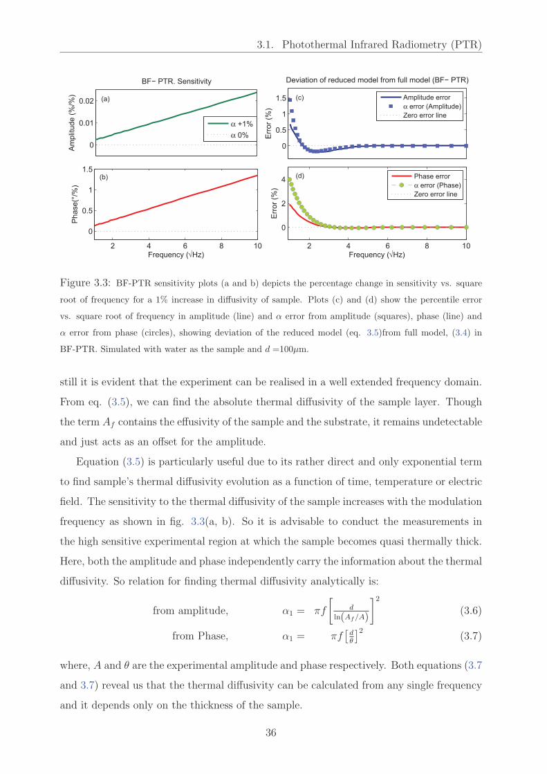
3.1. Photothermal Infrared Radiometry (PTR)
0
0.01
0.02
BF− PTR. Sensitivity
Am
plit
ude (
%/%
)
α +1%
α 0%
2 4 6 8 10
0
0.5
1
1.5
Frequency (√Hz)
Phase(°
/%)
0
0.5
1
1.5
Deviation of reduced model from full model (BF− PTR)
Err
or
(%)
Amplitude error
α error (Amplitude)
Zero error line
2 4 6 8 10
0
2
4
Frequency (√Hz)
Err
or
(%)
Phase error
α error (Phase)
Zero error line
(a) (c)
(b) (d)
Figure 3.3: BF-PTR sensitivity plots (a and b) depicts the percentage change in sensitivity vs. square
root of frequency for a 1% increase in diffusivity of sample. Plots (c) and (d) show the percentile error
vs. square root of frequency in amplitude (line) and α error from amplitude (squares), phase (line) and
α error from phase (circles), showing deviation of the reduced model (eq. 3.5)from full model, (3.4) in
BF-PTR. Simulated with water as the sample and d =100µm.
still it is evident that the experiment can be realised in a well extended frequency domain.
From eq. (3.5), we can find the absolute thermal diffusivity of the sample layer. Though
the term Af contains the effusivity of the sample and the substrate, it remains undetectable
and just acts as an offset for the amplitude.
Equation (3.5) is particularly useful due to its rather direct and only exponential term
to find sample’s thermal diffusivity evolution as a function of time, temperature or electric
field. The sensitivity to the thermal diffusivity of the sample increases with the modulation
frequency as shown in fig. 3.3(a, b). So it is advisable to conduct the measurements in
the high sensitive experimental region at which the sample becomes quasi thermally thick.
Here, both the amplitude and phase independently carry the information about the thermal
diffusivity. So relation for finding thermal diffusivity analytically is:
from amplitude, α1 = πf
[
d
ln(Af/A)
]2
(3.6)
from Phase, α1 = πf[
dθ
]2(3.7)
where, A and θ are the experimental amplitude and phase respectively. Both equations (3.7
and 3.7) reveal us that the thermal diffusivity can be calculated from any single frequency
and it depends only on the thickness of the sample.
36

3.1. Photothermal Infrared Radiometry (PTR)
3.1.2.2 Back PTR (B-PTR) :- For Simultaneous Detection of Diffusivity and
Effusivity
Alike back photopyroelectric (BPPE) technique [36, 80], the so called Back-PTR (B-PTR)
configuration posses high sensitivity and allows simultaneous detection of thermal diffusiv-
ity and effusivity of the sample. As in the case of BF-PTR, here also we are bounded to
some maximum range of modulation frequency. As shown in figure 3.2(b), the heat is gen-
erated at the backing-sample interface and the signal detection is from the CaF2-Sample
interface for both scans, the sample and reference scans. The normalized equation derived
from eq. (2.43) is given by:
ΓB(ω) =T1(ω, z = −d)T
′
1(ω, z = −d) =e′
1
e1
(
1 + b′
01
) (
1 + b′
21
)
eσ′
1d
(1 + b01) (1 + b21) eσ1d
[
1−ℜ′
0ℜ′
2e−2σ
′
1d
1−ℜ0ℜ2e−2σ1d
]
(3.8)
The variables with prime show the thermal parameters of the reference material and with-
out prime represent the sample.
0
0.5
1
1.5
2
Am
plit
ude (
% /
%)
B−PTR: Sensitivity plots
100
101
102
0
0.2
0.4
0.6
0.8
Frequency (Hz)
Phase (
° /
%)
e, α (+1%)
e: (+1%), α (0%)
α (+1%), e (0%)
Figure 3.4: Simulated plots of frequency dependent amplitude and phase of a typical liquid sample
(α1 =1.48 ×10⁻⁷m2s−1, e1 =650 Jm−2K−1s−1/2, d= 50µm) showing the percentile change in amplitude
(upper plot) and phase (lower plot) with +1% change in α1 and e1, (circles); +1% change in e1 keeping
0% change in α1 (dotted line with cross) and +1% change in α1 keeping 0% change in e1 (dashed line).
Figure 3.4 contains the simulations using equation (3.8) for the percentage variation
of the frequency dependent normalized amplitude and phase plotted with +1% change in
37

3.1. Photothermal Infrared Radiometry (PTR)
Table 3.1: Thermal parameters used for simulations.
Diffusivity Effusivity Conductivity
(m2s−1) (Jm−2K−1s−1/2) (Wm−1K−1)
CaF2 3.58 ×10⁻⁶ 5135 9.71 a
Quartz 8.4 ×10⁻⁷ 1590 —
Waterb 1.43 ×10⁻⁷ — 0.598
a Data sheet, Crystran Ltd. b Ref.[81] water at 20 0C.
thermal diffusivity and effusivity of a typical liquid sample (circles) (α1=1.48 ×10⁻⁷m2s−1,
e1 =650Jm−2K−1s−1/2) having thickness, d = 50µm, sandwiched between CaF2 top layer
and bottom glass substrate (table 3.1). The dotted line with cross shows a change in
thermal effusivity (e1) by +1% keeping original diffusivity (α1, 0%) while the dashed line
represents +1% change in diffusivity and original effusivity (e1, 0%).
The trends of these plots demonstrate that the sensitivity towards thermal diffusivity
of the sample is monotonically increasing with the increase in modulation frequency for
both the amplitude and phase. It is also evident that the amplitude is sensitive to the
thermal effusivity in the entire frequency range while the phase is sensitive only at the lower
frequency region. Apparently, for such measurements which needs a physical replacement
of the sample with a reference material, a varying proportionality factor (Af ) may be
needed to consider in the fitting domain in order to nullify the offset that can come in the
signal amplitude because of many reasons, restricts the use of amplitude alone for finding
thermal parameters. Thus, in this case, an effusivity sensitive phase data in the lower
frequency region is needed to determine both of the thermal parameters from eq. (3.8).
Further more, B-PTR gives the advantage of finding thermal diffusivity and effusivity
simultaneously from a single frequency for those measurements in which Af is kept fixed
(means: no physical sample-reference replacement). This is the case when the used ref-
erence material is the sample itself in a particular condition (ambient temperature, zero
applied electric field etc.) where its thermal parameters are known. It helps to avoid time
consuming frequency scans while preserving better accuracy. Sample’s thermal diffusivity
can be calculated from the phase and the effusivity from the combined amplitude and phase
signals. The analytical expression for sample’s thermal diffusivity, α1, and effusivity, e1, are
38

3.1. Photothermal Infrared Radiometry (PTR)
given by equations (3.9) and (3.10) respectively. Both of these equations are derived from
equation (3.8) considering that the sample is at quasi thermally thick (µs ≈ d) frequency
regime and thus the negative exponential term has negligible contribution (e−2σ1d ≈ 0).
α1 =
(
d√αrπf
d√πf − θ
√αr
)2
(3.9)
e1 =− 1
2
{
L−R +
√
(L−R)2 − 4J
}
(3.10)
where,
R =exp(θ)
erA
(
e2r + erL+ J)
L = e0 + e2 J = e0e2
A is the normalized amplitude and θ is the normalized phase. αr and er are thermal
diffusivity and effusivity of the reference material respectively. f represents the modulation
frequency and d is the sample thickness.
3.1.2.3 Front-PTR (F-PTR)
Rather easier but less sensitive than the rear detection involved models, this, so called
front-PTR configuration is depicted as in Fig. 3.2(a). The laser excitation and the signal
detection are from the same side (CaF2 face), at the interface between CaF2 (layer: 0 )
and Sample (layer: 1 ), of the sample cell assembly for both the sample and reference
scans. The temperature field at the sample surface (z = 0) is described by the eq. (2.41)
which is obtained from the surface absorption model. To avoid the use of a second reference
material and thereby minimizes errors due to possible distortions in the experimental setup
due to the sample-reference replacement and also uncertainties on the reference material’s
thermal properties, we have carried out the reference scan with the same sample with semi
infinite thickness. Hence it gives better accuracy on the results and provides the possibility
of measuring the absolute values of sample thermal parameters. The equation for F-PTR
model with sample of known thickness, d, normalised with same semi infinite sample is
obtained from eq. (2.41) and can be written as:
ΓF (ω) =1 + R2e
−2σ1d
1−R0R2e−2σ1d(3.11)
Figure 3.5 shows the frequency dependent procentile sensitivity variations of the nor-
malised amplitude and phase for 5% change in thermal diffusivity and effusivity, one by
39

3.1. Photothermal Infrared Radiometry (PTR)
−2
0
2
4x 10
−3
Am
plit
ude (
% /
%)
sensitivity plots; F−PTR
100
101
102
103
−0.2
−0.1
0
0.1
Frequency(Hz)
Phase (
° /
%)
α (+5%)
e (+5%)
α, e (+5%)
Figure 3.5: Frequency dependent sensitivity plots of the F-PTR model for the percentage change in
amplitude (upper plot) and phase (lower plot) for percentage change in thermal parameters. The solid
line represents a +5% change in sample thermal diffusivity without varying effusivity while the dashed line
corresponds to a change of +5% in effusivity keeping diffusivity same as reference. The circles represents
a change of +5% in both α and e. The simulation has been done for liquid sample with typical thermal
parameters (α1 =1.48×10⁻⁷ m2s−1, e1 =650 Jm−2K−1s−1/2) and d =30 µm with steel as backing and
CaF2 as the top layer. The normalisation has been done with the same sample while making it semi
infinite.
40

3.1. Photothermal Infrared Radiometry (PTR)
one and together, for a typical liquid sample having distinctive values of thermal parame-
ters (α1 =1.48×10⁻⁷ m2s−1, e1 =650 Jm−2K−1s−1/2). The sample is sandwiched between
a CaF2 window (layer-0) and a steel substrate (layer-2) holding thermal parameters as in
the table 3.1. Here the choice of steel substrate is because of its high thermal effusivity
that improves the sensitivity via the increased thermal mismatch between the sample and
backing. This configuration allows one to find out the thermal diffusivity and effusivity of
a liquid sample simultaneously knowing the thermal parameters of the surrounding layers
and the sample thickness. The zero crossing method [82] is also valid for finding the ther-
mal diffusivity of the sample from the normalised phase knowing only the thickness (d)
and zero crossing frequency (f(θ=0)) and is given by:
α1 =4d2f(θ=0)
π, n = 1, 2, 3... (3.12)
3.1.3 Photothermal Radiometry Experimental Set Up
The general procedure for conducting PTR experiments is relatively simple [65]. Like other
photothermal techniques [63], the sample under investigation is heated periodically at a
frequency, f = ω/2π, where ω is the angular frequency, using an intensity modulated laser
beam. These heat pulses diffuse into the sample layers and produce periodic temperature
variations, thus emitting infrared (IR) waves. These emitted IR signals are collected by
the aid of proper optical arrangements and focused into an IR detector. A lock-in ampli-
fier locked at the same modulation frequency of excitation quantify the output from IR
detector. As obtained signal contains both the thermal parameters of the sample layers
and the contribution from instrumental transfer function which comes from the underlying
electronic circuitry. A proper normalisation procedure allows one to filter out the signal
that depends only on thermal parameters of the sample layer system. Figure 3.6 shows the
schematic representation of a classical PTR set up.
3.1.3.1 From Laser Excitation to Infrared Detection
Laser source:- Laser beam of wavelength (λ =532 nm) corresponding to the green color
in the electromagnetic spectrum has been used as the source (manufacturer Laser Quantum,
He-Ne, Ventus HP 532, 1.4 mm spot size).
41

3.1. Photothermal Infrared Radiometry (PTR)
IR Detector
Laser
Beam Expander
Mirrors Parabolic
Mirror
Pre Amplifier
Lock in
Computer
Sample
Figure 3.6: Photothermal infrared Radiometry set up
Acousto-optic Modulator:- The laser module contains an internal modulator with a
maximum modulation frequency of about 10 kHz. For intensity modulations above this
frequency range, a separate acousto-optic modulator (IntraAction, AOM-40) was used.
Optical arrangements:- The Infrared signal coming out of the sample surface was
collected and focused by two parabolic gold coated mirrors (Edmund Optics, 90 DEG Off
Axis Parabolic, M2 R184613-10140). A telescopic lens arrangement with a magnification
factor of six has been used to make the spot size (8.4 mm) big enough to avoid three
dimensional effects at the experimental range of frequencies.
IR Detector:- A liquid nitrogen cooled HgCdTe Infrared detector (Judson Technologies,
Model: J15D12-M204-S01M-60; bandwidth: DC - 250 kHz) was used. Photograph from
an experiment showing the sample, detector and optical arrangements are displayed in fig.
3.7
3.1.3.2 Electronic Circuitry and Signal Recording
The detector signal was converted to voltage and pre amplified by PA 300 pre-amplifier.
This amplified signal was then connected to a Lock-in amplifier ( SIGNAL RECOVERY,
42

3.1. Photothermal Infrared Radiometry (PTR)
Figure 3.7: A photograph of the experimental setup
model: 7260, maximum oscillator frequency: 250 kHz). The Lock-in was connected to a
personnel computer via Agilent GPIB (General Purpose Interface Bus) card. The complete
experiment was automatized using LabVIEW software from National Instruments (NI).
Figure 3.8 is the LabVIEW front panel for controlling and recording the experiments
automatically.
3.1.3.3 Temperature Controlling
A home made heater powered by a programmable power supply (Instek, PSS-2005, 0-20V,
0-5A) was used for heating the sample cell. This helped to conduct experiments under
constant temperature as well as to carry out measurements under varying temperature. As
used temperature controller, controlled by a computer based PID (Proportional Integral
Derivative) controller, had the ability to regulate temperature better than 10 mK inside
the sample cell.
3.1.3.4 Electric Field Varying Experiments
For electric field varying measurements (e.g., liquid crystal re-orientation), signal from
a function generator (RIGOL, DG2021A) was amplified with a ×20 Voltage amplifier
(model:F20A) and applied to the sample cavity.
43

3.1. Photothermal Infrared Radiometry (PTR)
Figure 3.8: Front panel of the LabVIEW program used for the automation of experiments.
3.1.3.5 Cell for Liquid Samples
A 2.mm thick (24.mm diameter) CaF2 window (from Crystran, UK) having good infrared
transmission range (λ = 300nm to 10µm) was used as the top semi-infinite layer for all
the front and back experiments. While for the backing we have chosen special quartz
cuvettes (cells with detachable windows, type: QS 124, sample space thickness error ≤
±5%, from Hellma analytics), which in principle serves as the sample holder and gives
excellent accuracy over the sample thickness.
Figure 3.9: Photograph of the cell assembly used for liquid measurements using PTR technique
For all liquid measuring methods, sample heating by the laser absorption was achieved
by making thin opaque metallic coatings at both of the interfaces; sample-CaF2 and sample-
backing interfaces. These metallic coatings were also served as electrodes for the electric
field varying experiments. The thickness of these coatings were typically a few hundreds of
44

3.2. Validation of PTR Methods for Liquids
nanometers and assumed to have no effect on the normalized signal because these coatings
are thermally very thin in our experimental frequency range. It was also insured that
no incident laser beam was transmitted through the opaque coatings at the interfaces
validating the surface absorption model. Figure 3.9 shows the cell windows used for the
liquid experiments. The CaF2-Sample-backing assembly was mounted inside a 25 mm
holder and tighten together in order to maintain the sample thickness unchanged.
3.2 Validation Experiments on PTR Methods for
Measuring Thermal Properties of Liquid Samples
Verification of the PTR methods for thermal characterization of liquids described in sec-
tion 3.1.2 has been investigating firstly using water and glycerol as samples, which are
having well known thermal parameters. All the experiments were carried out at ambient
temperatures (20-22 0C). Experimental setup and the cell arrangements for liquid sample
encapsulation are described in section 3.1.3. The thermal parameters of the surrounding
layers and reference materials used for the normalisation procedure are given in table 3.2.
Table 3.2: Thermal parameters used as input data for fitting.
MaterialDiffusivity Effusivity Conductivity
(m2s−1) (Jm−2K−1s−1/2) (Wm−1K−1)
CaF2 3.58 ×10⁻⁶ 5135 9.71 a
Quartz 8.4 ×10⁻⁷ 1506 1.38
Waterb 1.43×10⁻⁷ 1581 0.598
Steel – 7535 –
a Data sheet, Crystran Ltd., b Ref.[81] water at 20 0C.
45

3.2. Validation of PTR Methods for Liquids
3.2.1 Results obtained with BF-PTR configuration
3.2.1.1 BF-PTR experiment with water
The normalized experimental amplitude and phase for water sample plotted as a function of
square root of modulation frequency is shown in figure 3.10. A least square fitting has been
done on the experimental amplitude, phase and complex (fitting amplitude and phase data
together simultaneously) data against theoretical model described in eq. (3.5) in order to
extract the thermal diffusivity of the sample under investigation. The best fitting results
corresponding to lowest χ2 values are given in table 3.3 together with other literature
values for comparison. The agreement of the results with the thermal diffusivity values
from literature support the validity of the method. The precision cells helped to minimize
the errors due to thickness uncertainties and which are neglected in the calculations.
10−1
100
Norm
alis
ed A
mplit
ude
BF−PTR
4 5 6 7 8 9
−250
−200
−150
−100
Square root of Frequency (√Hz)
Norm
alis
ed P
hase (
0)
Experiment
Best fit
Figure 3.10: Normalized BF-PTR signal amplitude (upper plot) and phase (lower plot), plotted as a
function of square root of the modulation frequency for water sample (d =100µm). The circles are from
the experimental data and the full line represents the best fit. CaF2 window is used as the top layer and
quartz cell as the backing.
Least Square Analysis and Error Calculation :
In table 3.3, the best fit values and their statistical uncertainties (σp) for diffusivity (α1)
(one of the fitted parameter) calculated from each type of experimental signals (amplitude,
phase and complex) are presented. The χ2 cost function is calculated by:
46

3.2. Validation of PTR Methods for Liquids
Table 3.3: Thermal Diffusivity from BF-PTR.
Sample
BF-PTR
LiteratureAmplitude Phase Complex
fitting fitting fitting
10−7(m2s−1) 10−7(m2s−1)
Water 1.441±0.005 1.435± 0.006 1.436± 0.006 1.437±0.008a , 1.43b
E.G 0.926±0.006 0.924±0.007 0.922±0.009 0.918±0.002c
Lanolin 0.50±0.02 0.49±0.02 0.53±0.03 —
a[45] at 250C; b[81] at 20 0C; c[83].
χ2 =1
N
N∑
j=1
[Γexp (ωj)− Γtheory (ωj,p)]2 (3.13)
with N , the number of summed quadratic differences of the experimental and theoretical
values; ωj(j = 1...N), the experimentally available frequencies; Γexp (ωj), is the normalized
experimental signal; Γtheory (ωj,p), corresponding theoretical normalized signal. p is the
set of fitting parameters. Least square analysis finds best set of fit parameters by varying all
of them (fit parameters) so that a lowest χ2 value is achieved. Then the fitting uncertainty
σp for each fit parameter, e.g. α1, is calculated by varying its value around the best fit
while keeping all other parameters constant.
σp =
√
2
(N − P ) ∂2
dp2(χ2(p)/χ2(p0))
(3.14)
Here, p0 is the optimised set of fitted parameters corresponding to the lowest χ2 value
obtained from the least square analysis and p is the set of parameters containing the
varying parameter for which the uncertainty to be calculated. In eq. (3.14), the second
order partial derivative of χ2 function was obtained by fitting a parabola through χ2(p),
where p is the varying parameter during the χ2 analysis. The steepness of this parabola is
inversely proportional to the fit parameter’s uncertainty.
Interestingly the small values of the uncertainties comparable with the PPE measure-
ment results represent the high sensitivity of the method and quality of the experimental
47

3.2. Validation of PTR Methods for Liquids
1.42 1.44 1.46
x 10−7
0.05
0.1
0.15
(1.441+/−0.005)10−7
χ2
α (m2s
−1)
1.42 1.44 1.46
x 10−7
1
1.5
2
x 10−3
(1.435+/−0.006)10−7
α (m2s
−1)
1.42 1.44 1.46
x 10−7
1
1.5
2
(1.436+/−0.006)10−7
α (m2s
−1)
(b) (c)(a)
χ2 analyses (BF−PTR, water sample)
Figure 3.11: χ2 analyses in the neighbour hood of its minimum for calculating the statistical uncertainty.
Analyses on amplitude (a); phase (b); and on complex (c) data.
signal. The experimental results on ethylene glycol (E.G) and lanolin (wool wax)[84] are
also included in table 3.3.
3.2.1.2 BF-PTR experiment on 5CB with varying electric field
Liquid Crystals and their Physical Characteristics :
Liquid crystal (LC) compounds are special class of materials exhibiting crystal ordering
in liquid state. Because of such unique property, LCs unfolded improved class of optical
devices which are thin, light in weight and even foldable. Thermodynamically, this liquid
crystalline phase exists in between the melting point and the isotropic clearing tempera-
ture of material. Ordinarily, LCs may display one or more mesophases depending on the
molecular symmetry and three major classes of these mesophases are: nematic, smectic
and cholesteric. The differences between these mesophases are coming from their lattice
order parameter.
Nematic liquid crystals tend to align themselves parallel to one another along an ar-
bitrary principle axis (n). While cholesteric phase happens when there is a “twisting” of
the nematic director between consecutive layers, usually in helix form. In smectic phase,
the molecules align parallel to one another within a layer and inter layer translational
movements are restricted. Figure 3.12 schematically explains these LC phases.
Liquid crystals in its crystalline phase are opaque and turbid fluid to our naked eye
but it shows characteristic optical textures due to its strong birefringence property when
looking through a polarizing microscope. In normal form, direction of the director, n,
48

3.2. Validation of PTR Methods for Liquids
can be in any arbitrary direction within the mesophase. Interestingly, these directions
and thereby their properties can be controlled by different ways, e.g, rubbing or surface
treatment of the material in contact, applying electric or magnetic field etc. These unusual
optical properties and the possibility to control it have attracted the scientific world to use
it in various areas.
Nematic phase Smectic phase Cholesteric phase
n n
Figure 3.12: Three of the main liquid crystal phases.
Here, we have studied the vari-
ations of 5CB liquid crystal ther-
mal diffusivity under varying elec-
tric field (EF) (sinusoidal elec-
tric field of fixed frequency (fe)=
1kHz was chosen to avoid polariza-
tion field effects at LC-electrode
boundaries). Figure 3.13 shows a
schematic representation of liquid
crystal molecular alignment before
and after the application of an ap-
plied electric field. When the LC sample is sandwiched between the cell walls, all the
molecules take the direction parallel to the cell wall. This alignment depends on the sur-
face characteristics of the cell surface in contact with LC. Different chemical and physical
treatments governs the LC molecular alignment. Since the thermal transport properties
are anisotropic in LC materials, the heat transport is maximum in the direction of the
molecular alignment axis or director (n). So, if n is parallel to the cell wall (like in fig.
3.13(a)), the thermal conductivity normal to the cell wall (normal to n) is lower than that
in the parallel direction. Now, upon the application of a sufficiently strong electric field,
the LC molecules try to align in the direction of EF, normal to the cell walls. Thus the
thermal conductivity also increases in this direction.
Experimental Results on 5CB Liquid Crystal :
Laser intensity modulated frequency scans for different applied electric fields on LC
sample were conducted for finding thermal parameters. Normalisation for each back fre-
quency scan has been done with the corresponding front frequency scan. The results were
obtained by fitting the normalized experimental signals using equation (3.5). In practice,
49

3.2. Validation of PTR Methods for Liquids
Figure 3.13: LC molecules under zero and an applied electric field.
a single front frequency scan serves the purpose as the normalisation signal for all the back
scans because, the front signals are less sensitive to the variation of the sample’s thermal
parameters and thus resulting in similar or same amplitude and phase values in all the
front scans. It is also worthy to mention that the scans were done near to sample’s quasi
thermally thick regime, where the experimental signal is most sensitive to the sample’s
thermal diffusivity. The experiment has been carried out around ∼ 28 0C (nematic phase:
25 0C - 35 0C). The LC is dropped into the sample holder and heated above 35 0C, until its
clearing temperature, before closing the cell for the experiment. Our results on the electric
field dependent thermal diffusivity of 5CB are shown in figure 3.14.
The thermal diffusivity variation is about 9% without doing any pre surface treatments
which is necessary to obtain high degree planar alignment and thereby increased thermal
parameter contrast [85]. This behaviour of the thermal diffusivity of 5CB as a function of
electric field is similar to the one obtained with PPE in reference [23].
3.2.2 Results obtained with B-PTR configuration
3.2.2.1 B-PTR experiment on glycerol
Back-PTR (B-PTR) method has the advantage of getting thermal diffusivity and effusivity
of liquid samples simultaneously with high certainty. Figure 3.15 shows the frequency
dependent experimental result on glycerol (sample) normalized with water (reference).
The thermal parameters used for the reference liquid are from table 3.2. The experimental
data (amplitude, phase and complex) have been fitted with equation (3.8) to obtain the
thermal diffusivity and effusivity. The results obtained for the best fitting values of glycerol
50

3.2. Validation of PTR Methods for Liquids
0 0.2 0.4 0.6 0.8 18.6
8.8
9
9.2
9.5x 10
−8 Diffusivity with errorbar vs. E.Field (5CB)
Electric Field (Vrms
/µm)
α (
m2s
−1)
Figure 3.14: Variation of thermal diffusivity of 5CB liquid crystal ( at 28 0C) vs. varying electric field
(sinusoidal, 1kHz) from the BF-PTR experiment.
with statistical uncertainties are shown in table 3.4 and these results are in good agreement
with the already reported values. For checking if the obtained set of values having any
pair wise fitting dependency, we have performed a contour map for the χ2 cost function vs.
α and e as in figure 3.16(a). It shows closed curves around the best fitting pair of values
which confirms the absence of any interdependency between the two thermal parameters.
Most Squares Inversion and Multi-Fold Degeneracy :
Assessment of two fold degeneracy (between any two fitting parameters) can be brought
out by plotting contour plots but a three fold or higher (multi fold) degeneracy cannot be
viewed in 2-D plots. Here a third fitting parameter called proportionality factor (Af )
which comes from the sample-reference replacement (Af has effect only on the amplitude
and not on the phase. A possible reason for including Af is coming from the small changes
in absorbed laser intensity due to the sample cell rearrangements which can alter the
amount of photothermal heat generation) may introduce the chances to have a three fold
degeneracy (same results for different sets of input parameters) between the three unknown
fitting parameters (α, e and Af ). It can be brought out by doing so called “Most Squares
51

3.2. Validation of PTR Methods for Liquids
Table 3.4: B-PTR and F-PTR Experimental results on Glycerol.
MethodDiffusivity Effusivity
×10−8(m2s−1) (JK−1m−2s−1/2)
B-PTR
Amplitude fit 9.45 ± 0.02 958 ± 2
Phase fit 9.425 ± 0.007 940 ±10
Complex fit 9.43 ± 0.02 945 ± 3
F-PTR Complex fit 9.5 ± 0.3 945 ±11
Ref.[81] (250C) 9.99 923
0.4
0.5
0.6
0.7
0.8
Norm
ais
ed A
mplit
ude
B−PTR Experiment on Glycerol Sample
100
101
102
−40
−30
−20
−10
0
Frequency (Hz)
Norm
alis
ed P
hase (
°)
Full Experimental Data
Fitted Region
Fit
Figure 3.15: Experimental result on glycerol (sample) normalized with water (reference) plotted as a
function of f . Amplitude (upper plot) and phase (lower plot) are fitted simultaneously. The symbols show
the experimental curve and the full line represents the best fit (d=50µm).
52

3.2. Validation of PTR Methods for Liquids
Inversion” [45, 86]. In classical least-squares error analysis procedure (described in section
3.2.1.1), each parameter vary around its best fit value keeping all other parameters fixed
unambiguously and calculates the error. While in the case of most squares error analysis,
each chosen value of a selected parameter (e.g., α) around its best fit is optimized by varying
all other fitted parameters until minimizing the χ2 cost function. So, for each value of the
selected parameter, an additional least square analysis by minimizing the χ2 cost function
is being carried out in order to optimize the full set of fit parameters. The results from the
most squares analysis can be analysed as in the following way. If the analysis shows a single
minimum, which means that the obtained set of values are unique. On the other hand if it
shows a flat line, it indicates a multi-fold degeneracy which means that the fit parameter
set satisfies more than one solution for the same experimental data. Figure 3.16(b, c)
shows the least square and most-squares analysis for the thermal diffusivity and effusivity.
The parabolic shape of the plots indicate the absence of degeneracy with all other fitting
parameters for each of these thermal quantities. The sharpness of the parabola is a proof
of lower statistical uncertainty and high accuracy of the experimental method. From fig.
3.16(b, c) it can be noted that the most squares curves are broader than the χ2 curves.
This is because the most squares analysis take into account of covariance with the other
fitting parameters.
9.3 9.45 9.6
x 10−8
1
2
α (m2s
−1)
χ2 /
χ2 min
imum
875 950 1025
1
2
e (JK−1
m−2
s−1/2
)
Contour plot
α (m2s
−1)
e (
JK
−1m
−2s
−1/2
)
4.2e−0050.000168
0.000168
0.000168
0.000168
0.00
0.0006729.3 9.4 9.5 9.6
x 10−8
900
930
960
990
χ2
Most square(a) (b)
Most squares Error analysis
(c)
Figure 3.16: Contour plot (a) showing the closed curves with χ2 minima around the best fitting values
of α and e confirms the absence of degeneracy. Most square error analysis (full line) plotted along with
the least-square (dashed line) for thermal diffusivity (b) and effusivity (c) confirming that the results are
unique. The statistical uncertainty is inversely proportional to the sharpness of the parabolic minima. The
analysis is for the B-PTR experiment (fig. 3.15) with glycerol as sample and water as the reference.
53

3.2. Validation of PTR Methods for Liquids
3.2.2.2 B-PTR experiment on 5CB with varying electric field
0.8
0.9
1
B−PTR, 5CB − Electric Field Varying Experiment
Norm
alis
ed A
mplit
ude
5.5 6 6.5 7
−8
−6
−4
−2
0
Square root of Frequency (√Hz)
Norm
alis
ed P
hase (
°)
EF=4mV/µm EF=60mV/µm EF=1V/µm
Figure 3.17: Normalized experimental signals (symbols) and the best fits(lines) are plotted vs. laser
modulation frequency for 5CB liquid crystal sample under three different electric fields. Signals are fitted
to obtain α and e keeping Af fixed. The reference signal was from the sample at zero electric field.
Employing B-PTR experimental method, we have also investigated the variations of
α and e for 5CB liquid crystal sample with varying electric field. The obtained results
are from the scans performed at high sensitive frequency region, where the sample was
in quasi thermally thick regime. The frequency scan at zero electric field was taken as
the reference signal for normalisation for all other signals with applied electric field, thus
the Af kept fixed. The reference thermal parameters for the 5CB at zero electric field for
thermal diffusivity was from the BF-PTR result on 5CB and for the effusivity was from
reference[23]. Figure 3.17 shows the typical normalized experimental signals as a function
of frequency for three different electric fields. The normalized signals were fitted using
equation (3.8) and figure 3.18 shows the obtained thermal diffusivity and effusivity values
plotted as a function of applied electric field.
3.2.2.3 B-PTR experiment on 5CB with varying temperature
Depending on the temperature, liquid crystal materials show different phases such as crys-
talline (C), smectic (Sm), nematic (N), isotropic (I) etc. So the thermal transport prop-
54

3.2. Validation of PTR Methods for Liquids
0 0.2 0.4 0.6 0.8 18.6
8.8
9.2
9.6x 10
−8
Electric Field (Vrms
µm−1
)
α (
m2s
−1)
B−PTR: Thermal Diffusivity and Effusivity vs. Electric Field (5CB)
0 0.2 0.4 0.6 0.8 1560
580
600
620
Electric Field (Vrms
µm−1
)e (
JK
−1m
−2s
−1/2
)
(b)(a)
Figure 3.18: Variation of thermal diffusivity,(a) and thermal effusivity,(b) with error bar of 5CB liquid
crystal as a function of electric field. Results from B-PTR experiments done at 28 0C.
erties are also different in these phases. Moreover, on the transition from one phase to
another, different transport properties show continuous or discontinuous transitions due to
the change in its molecular order parameter. Here, we are investigating the widely studied
temperature dependent N-I transition in 5CB for validating B-PTR method.
Since B-PTR has the advantage of finding thermal diffusivity and effusivity simultane-
ously from a single frequency for those measurements in which Af is kept fixed, it helps to
avoid time consuming frequency scans while preserving better accuracy. Sample’s thermal
diffusivity can be calculated from the phase and the effusivity from the combined amplitude
and phase signals considering the sample is at quasi thermally thick (µs ≈ d) frequency
regime where the negative exponential term in equation (3.8) can be approximated to zero
(e−2σ1d ≈ 0). The analytical expression for α and e are given by:
αs =
(
d√αrπf
d√πf − θ
√αr
)2
(3.15)
es = −1
2
{
L−R +
√
(L−R)2 − 4J
}
(3.16)
where,
R =exp(θ)
erA
(
e2r + erL+ J)
L = ec + eb J = eceb
55

3.2. Validation of PTR Methods for Liquids
and A is the normalized amplitude and θ is the normalized phase. er, es, ec and eb are the
thermal effusivities of reference, sample, CaF2 window and backing respectively. αs and αr
are the thermal diffusivities of sample and reference respectively. f represents the modu-
lation frequency and d is the sample thickness. Figure 3.19 shows the variation of thermal
diffusivity, effusivity and conductivity (calculated from α and e) vs. temperature for the
5CB liquid crystal. The temperature dependent experimental signal was normalized with
the signal at the isotropic phase and the reference values were chosen from reference[85].
The experiment has been done with a single stage temperature controller with temperature
resolution better than 10 mK.
4
6
8
x 10−8 B−PTR (N−I phase transition of 5CB)
α (
m2s
−1)
500
600
e (
JK
−1m
−2s
−1/2
)
25 30 35 40 43
0.13
0.16
Temperature (°C)
κ (W
m−
1K
−1)
(c)
(b)
(a)
Figure 3.19: Experimental results on variations of thermal diffusivity (a), thermal effusivity (b) and
thermal conductivity (c) from the temperature varying B-PTR experiment around the Nematic - Isotropic
(NI) phase transition of 5CB. The experiment has been done at f =32Hz (laser modulation frequency)
and d =36µm. The thermal conductivity has been calculated from e and α.
3.2.3 Results obtained Using F-PTR configuration
In order to validate F-PTR method, we have measured thermal diffusivity and effusivity
of glycerol. The experiment has been conducted as described in section 3.1.2 and the
56

3.2. Validation of PTR Methods for Liquids
normalisation has been done with the same semi infinite sample. The results on glycerol as
the sample are included in table 3.4. The sample is sandwiched between the CaF2 window,
which acts as the semi infinite top layer, and a highly effusive steel backing in order to obtain
better sensitivity to sample’s thermal parameter changes. The sample space is created by
an O-ring shaped mica film and placed in between the top layer and the backing. The
thickness of the sample space has been calibrated using water as the sample having known
thermal parameters as indicated in table 3.2. The normalised experimental amplitude and
phase plotted as a function of modulation frequency, as shown in fig. 3.20, are fitted using
eq. (3.11).
0.92
0.94
0.96
0.98
Norm
alis
ed A
mplit
ude
F−PTR , Glycerol Sample
102
103
−2
0
2
4
Frequency (Hz)
Norm
alis
ed P
hase (
°)
Figure 3.20: Normalized experimental signal for Glycerol sample (d =38µm) using F-PTR plotted as a
function of laser modulation frequency. Normalisation has been done with semi infinite sample. Circles
show the experimental data and the full line represents the best fit.
The obtained results from our experiments are in good agreement with the already
reported values and also with the results obtained with B-PTR experiments. The un-
certainties in the experimental results, obtained from the least squares error analysis by
minimizing the χ2 cost function, for each thermal parameters, are also included in table
3.4. Since this configuration has less sensitivity towards sample’s thermal parameters, the
results have bigger uncertainties than the results from BF-PTR or B-PTR configurations.
57

3.3. PDLC Results
3.2.4 Plausibility of PTR Methods for Characterizing Liquid
Sample’s Thermally
Until now, the most used method for liquids thermal characterization is probably the PPE
calorimetry. The main advantage of this method compared to other PT techniques is its
simplicity: it measures directly the temperature variation of the sample with the special
feature for liquids of a perfect liquid/pyroelectric sensor thermal contact. In this work, we
propose the PTR technique as an alternative calorimetry. Concerning the accuracy of the
investigations, in both techniques, when using sandwiched detection cells, it was demon-
strated [70, 44] that it is connected with the values of the thermal parameters of the layers
of the detection cell; more exactly, the accuracy is increased when the values of the thermal
effusivity of the liquid and backing layers are close. In the PTR configurations proposed
in this work, the backing layer is glass with a thermal effusivity rather close to the typical
liquids, so the experiment is optimized in order to obtain high accuracy. While considering
the signal to noise ratio, PPE outperforms PTR, which limits the temperature resolution
granted by the PTR in highly resolved temperature dependent measurements. Some re-
cent advances in IR detection technologies promising us improved sensing possibilities [87]
which in principle allows to perform experiments at extremely low laser powers than it
requires now. The requirement of IR transparency of the first layer of the proposed PTR
detection cell can be easily fulfilled, a lot of commercially available materials satisfying this
criterion.
3.3 Thermal Transport Studies in Polymer Dispersed
Liquid Crystals (PDLC) Under Frequency Depen-
dent Electric Field
Polymer Dispersed Liquid Crystals (PDLCs) are the subject of study in our lab for the
past few years. Until now only the different aspects governing the thermodynamic of
the phase separation and the electro-optical performances (transmission properties, drive
voltage, switching times, etc.) of these materials have been extensively investigated. The
studies on thermal transport properties of PDLC samples can be very interesting in this
58

3.3. PDLC Results
heterogeneous material composite. We have used the PTR technique developed for liquid
studies to determine the thermal behaviour of the PDLC systems under applied electric
field.
PDLCs are modified edition of the conventional LC technology. These are made up of
micron or sub-micron sized LC droplets encapsulated inside a polymer matrix. One of the
usual procedure of preparation is in-situation polymerization of host polymer matrix in the
presence of LC proceeded by phase separation. This manufacturing procedure is especially
simple and avoids the requirements of surface aligning or cell filling and sealing which
are needed in the case of twist cells. Conventional LC (super twist cells, twisted nematic
(TN) cells, π-cell) needs the use of polarisers while PDLC’s do not require any polarisers.
It particularly reduces the power loss due to the absence of polarisers (polarisers absorb
∼ 50% incident light in LC cells) and thereby increases the device efficiency. Moreover, in
high temperatures, polarisers often degrade or peel off. Sturdy environmental properties,
fast switching time and low production costs are other attractions of PDLC technology.
Some of its electro-optical applications are: flexible displays [88, 89, 90], window shutters,
projection displays [91], optical switches [92], focus tunable lenses [93] etc.
Figure 3.21: PDLC before and after applying electric field E.
The downward arrows showing the light path.
The principle of operation
is based on the electric field-
controlled optical transmission
properties of the composite mate-
rials sandwiched between two
transparent conducting elec-
trodes. Light is efficiently scat-
tered in the initial off-state (zero
field) because of the refractive
index mismatch between the
droplets and the matrix. Appli-
cation of electric field causes the
LC molecules to orient within
the droplets and if the ordinary
refractive index of the LC matches
that of the matrix a high degree
59

3.3. PDLC Results
of transparency can be achieved (fig. 3.21). Upon removal of the voltage, the droplets
return to their original random orientation inducing light scattering.
3.3.1 Maxwell-Wagner-Sillars Effect
Polymer dispersed liquid crystal assembly is a heterogeneous mixture of LC and polymer.
Because of the difference in dielectric characteristics (ability to hold charges) and electrical
conductivities in these material mixture components, an additional charge polarisation
occur at each LC-polymer boundaries upon the application of an EF as in fig 3.22. At
lower frequencies, the blocking inner charges at the boundaries start to build up and
produce reduction in the equivalent applied EF strength. This interfacial polarisation
effect, also known as Maxwell-Wagner-Sillars (MWS) effect [94, 95] in a multiple phase
mixture, vanishes at sufficiently high frequencies of applied EF at which the movement of
charges become frozen out and the development of depolarisation field interrupts.
Figure 3.22: Maxwell-Wagner-Sillars effect in a het-
erogenious medium
Since this effect crucially affects electro-
optical properties of such heterogeneous
systems, a clear understanding of such
properties are important in the application
point of view. Several authors have studied
this interfacial effects and its consequences
in electro-optic properties are reported [96,
97, 98]. Boussoualem et al [99, 100]
conducted differential scanning calorimetry
(DSC), dielectric spectroscopy and electro-
optic studies on polystyrene PS/ (4,4’-
octylcyanobiphenyl) 8CB and PS/5CB dis-
persed systems and reported frequency de-
pendent behaviour attributed to the MWS effect in such mixtures. Their electro-optic
studies were showing the variation of light intensity vs. frequency (fe = ωe/2π) of the
applied electric field and which were explained in terms of MWS effect by considering the
self consistent field approximation for calculating the electric field (Edrop) inside a spherical
60

3.3. PDLC Results
droplet under sinusoidal field [101, 102], which is given by:
Edrop(ωe) =3ǫ⋆M
ǫ⋆LC + 2ǫ⋆M − φLC (ǫ⋆LC − ǫ⋆M)Eae
−iωet (3.17)
and,
ǫ⋆M = ǫ′M − iσMωeǫ0
(3.18)
ǫ⋆LC = ǫ′LC‖ − iσLC‖
ωeǫ0(3.19)
where,
φLC ⇒ Phase separated LC fraction.
Ea ⇒ Magnitude of the applied electric field.
ǫ′M ⇒ Dielectric permittivity of polymer matrix
ǫ′LC‖ ⇒ Dielectric permittivity of LC aligned with Ea
σLC‖ ⇒ Electrical conductivity of LC in the direction of Ea
σM ⇒ Electrical conductivity of Polymer matrix in the direction of Ea
Inside PDLC, a part of the LC dissolves into the polymer. The amount of LC which
dissolves into the polymer is defined as solubility limit (β) and it can be found by doing
DSC measurements. The undissolved part will form droplets. Knowing β and the amount
of LC added to the polymer, x, one can calculate the phase separated LC fraction (φLC)
using [103, 104, 105]:
φLC =100
x
x− β
100− β, x > β (3.20)
where, all the quantities are in weight percentage. Value of β is about 55% at room
temperature has been used to calculate φLC using eq. (3.20) for finding the amount of LC
droplet phase separated inside the polymer matrix.
In this section, we are analysing the MWS effect on dynamic thermal properties of
PS/5CB composites and model it using eq. (3.17). Since the improved PTR methods
for measuring liquid samples are capable of measuring thermal parameters with enough
resolution, we have chosen B-PTR method (section 3.2.2) for experimental characterisation
of the PDLC system. Because of the non-contact capability of the PTR technique, the
measured thermal informations are free from electric field induced errors compared to
contact techniques, for which, the signal can be affected by the electric field applied to the
PDLC and making the measurements more tricky.
61

3.3. PDLC Results
Heat F
low
(a.u
.)
Figure 3.23: Thermogram of pure 5CB, showing crystalline (C) , Nematic (N) and Isotropic (I) phases
of 5CB liquid crystal. Figure obtained from reference [20]
3.3.2 Thermophysical, Electrical and Dielectric Properties
Polymer Dispersed Liquid Crystal (PDLC) samples were prepared using polystyrene (PS)
(Aldrich, molecular weight of 44000 g/mol as the polymer matrix and 5CB (Merck) as
inclusion with two different volume ratios of LC:PS (85:15 and 73:27). Some of the advan-
tages of PS compared to other thermo- plastic compounds are: very low ac conductivity
(σac ≈ 10−9 S/m), uniform dielectric permittivity (ǫ′
M ∼ 2.5) in both temperature (250C -
800C) and frequency [106, 81].
The density (ρ) of PS and 5CB are ≈ 1 (ρPS = 1.047 kg/m3 and ρ5CB = 1.008 kg/m3).
Dielectric permittivity and ac electrical conductivity of 5CB are: ǫ′
LC‖ = 10 and σLC‖ =
10−8 S/m [107, 108]. Figure 3.23 shows the phase diagram of pure 5CB and displaying the
temperature range of nematic phase between 230C to 350C. Thermal conductivities of PS
(κm = 0.11 W/mK) and 5CB aligned in parallel (κLC‖ = 0.24 W/mK) and perpendicular
(κLC⊥ = 0.12 W/mK) used are taken from references [109, 85]
3.3.3 Chemical Synthesis
PDLC was prepared by dissolving liquid crystal and polymer in solvent and evaporating the
solvent completely afterwards. 5CB and PS monomers in required amounts were dissolved
in equal amount of chloroform firstly. After completely dissolving both 5CB and PS in
chloroform, the mixture was placed in an oven and allowed for a complete evaporation
of chloroform for more than 24 hours to obtain a final PDLC sample. Upon the solvent
62
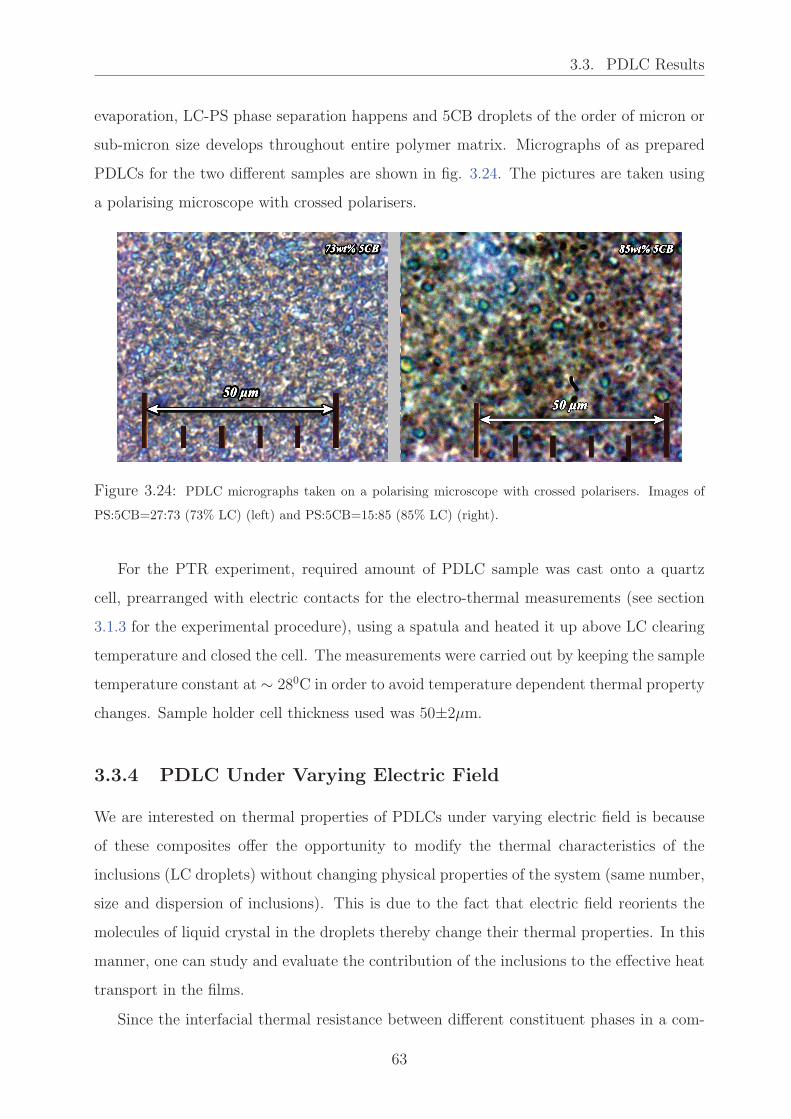
3.3. PDLC Results
evaporation, LC-PS phase separation happens and 5CB droplets of the order of micron or
sub-micron size develops throughout entire polymer matrix. Micrographs of as prepared
PDLCs for the two different samples are shown in fig. 3.24. The pictures are taken using
a polarising microscope with crossed polarisers.
Figure 3.24: PDLC micrographs taken on a polarising microscope with crossed polarisers. Images of
PS:5CB=27:73 (73% LC) (left) and PS:5CB=15:85 (85% LC) (right).
For the PTR experiment, required amount of PDLC sample was cast onto a quartz
cell, prearranged with electric contacts for the electro-thermal measurements (see section
3.1.3 for the experimental procedure), using a spatula and heated it up above LC clearing
temperature and closed the cell. The measurements were carried out by keeping the sample
temperature constant at ∼ 280C in order to avoid temperature dependent thermal property
changes. Sample holder cell thickness used was 50±2µm.
3.3.4 PDLC Under Varying Electric Field
We are interested on thermal properties of PDLCs under varying electric field is because
of these composites offer the opportunity to modify the thermal characteristics of the
inclusions (LC droplets) without changing physical properties of the system (same number,
size and dispersion of inclusions). This is due to the fact that electric field reorients the
molecules of liquid crystal in the droplets thereby change their thermal properties. In this
manner, one can study and evaluate the contribution of the inclusions to the effective heat
transport in the films.
Since the interfacial thermal resistance between different constituent phases in a com-
63

3.3. PDLC Results
posite can play a critical role in the thermal behaviour of composite systems, the effect of
this thermal resistance on the effective thermal conductivity of PDLC with different liquid
crystal concentrations has been studied.
Firstly, we have investigated the variation of thermal parameters of both PDLC samples,
(85% LC and 73% LC) under varying electric field at constant frequency (fe = 1 kHz) and
the results are depicted as in fig. 3.25.
0 0.1 0.2 0.3 0.4 0.5
0.12
0.14
0.16
0.18
Electric Field (Vrms/µm)
κ (W
m−
1K
−1)
6.5
7
7.5
8
8.5
9
9.5
10x 10
−8
α (
m2s
−1)
PDLC Thermal parameters under varying Electric Field
460
490
520
550
580
e (
JK
−1m
−2s
−1/2
)
PDLC73%
PDLC85%
PDLC73%
PDLC85%
PDLC73%
PDLC85%
Figure 3.25: Variation of thermal diffusivity (top) , thermal effusivity (middle) and thermal conductivity
(bottom) vs. varying electric field (at constant frequency (fe), 1kHz) for PDLC samples (85% LC and
73% LC).
The PTR experiments were conducted by fixing the laser modulation frequency, f =
64

3.3. PDLC Results
18Hz, at which the sample is in quasi-thermally thick regime, and varying EF strength
successively. The displayed results are from the mean of three consecutive EF scans. We
have also made an additional filtering by plotting volumetric heat capacity (ρC = e/√α)
and by taking data points lie within ±1% or ±0.55% (depending on the population of
experimental data points) from the linear fit value of ρC as shown in fig. 3.26. Here,
the behaviour of ρC is independent of the applied electric field as expected. The molec-
ular reorientation in LC do not make any contributions towards ρC and hence it stays
unchanging. Nevertheless, liquid crystal concentration changes produce difference in ρC
values.
The behaviour of the thermal conductivity (fig. 3.25) is intimately linked with the
reorientation of molecules in LC droplets. At zero field, the symmetry axis of each LC
droplet in the nematic phase varies randomly and for the heat entering the film, the effective
thermal conductivity is reduced. At high fields, each droplet’s symmetry axis is aligned
with the external field which is parallel to the heat flow. The thermal conductivity of the
droplets increases leading to an increase of the effective thermal conductivity of the PDLC
film.
0 0.1 0.2 0.3 0.4 0.5
1.76
1.78
1.8
1.82
1.84
1.86
x 106
Electric Field (Vrms/µm)
ρC (
Wsm
−3K
−1)
73% Experiment filtered (±0.55%)
Linear fit
0 0.1 0.2 0.3 0.4 0.51.78
1.8
1.82
1.84
1.86
1.88
1.9
1.92x 10
6
ρC (
Wsm
−3K
−1)
ρC from EF varying Experiments
85% Experiment filtered (±1%)
Linear fit
Figure 3.26: ρC plotted as a function of EF for both concentrations of PDLCs. Experimental data
points shown are within ±1% for 85% LC and ±0.55% for 73% LC from the mean value of ρC.
65

3.3. PDLC Results
3.3.4.1 Effective Medium Theory and Interfacial Thermal Resistance:
In all heterogeneous mixtures, thermal transport is hindered by interfacial boundaries.
Nan et al [110] has given an estimation of effective thermal conductivity (κPDLC) of such
heterogeneous mixtures with spherical inclusions on the basis of effective medium approach
by taking into account of interfacial thermal resistance:
κPDLC = κmκLC (1 + γ) + 2κm + 2φLC [κLC (1− γ)− κm]
κLC (1 + γ) + 2κm − φLC [κLC (1− γ)− κm](3.21)
where, γ = rk/rd, is the ratio of Kapitza radius (rk) and mean droplet radius (rd). κm
and κLC are thermal conductivities of polymer matrix and LC respectively.
γ is a dimensionless parameter which compares the Kapitza radius rk to the droplet
radius rd. The Kapitza radius is related to thermal interfacial resistance and describes
the transition when interfaces begin to play a significant influence on the effective thermal
conductivity of PDLC. When γ ≪ 1 the influence of the interfaces may be ignored but
if γ > 1 the contribution of the interfaces to the effective thermal conductivity becomes
more important than that of the volume of the inclusions.
By knowing the thermal conductivities of polymer matrix and LC as well as by experi-
mentally finding κPDLC and φLC (eq. (3.20)), one can calculate γ by rearranging eq. (3.21),
which is given by:
γ =κm
κPDLC
(κLC + 2κm + 2φκLC − 2φκm)− κLC − 2κm + φκLC − φκm
2κLC + φκLC + 2κmκLC
κPDLC
(φLC − 1)(3.22)
Equation (3.22) allows to compute rk, once we know the mean radius of the droplets.
Apparently, fig. 3.24 may not be sufficient to calculate the size of the droplets precisely.
However, a rough estimation of droplet diameters lie around 1 to 5µm for 85% LC and 0.5
to 2µm for 73% LC, from the figure.
Nematic droplets in our system possess the bipolar configuration, at zero field the
nematic is aligned tangentially at the droplet wall (fig. 3.27.a). Upon application of the
field, the nematic within the center of each droplet aligns quickly with the field. This
process leads to a droplet where the bulk of the nematic is aligned with the applied field,
but near the wall of the droplet the nematic molecules are still aligned tangentially to
the droplet surface (fig. 3.27.b). The orientation of the molecules along the surface of
66

3.3. PDLC Results
the droplets remaining unchanged in the presence and in the absence of the electric field
brought us to consider that the thermal interfacial resistance is constant and independent
of the electric field. For calculating γ, we have used thermal conductivities when the
LC molecules aligned in the direction parallel to the EF, at which κPDLC = κPDLC‖ and
κLC = κLC‖.
Figure 3.27: Schematic of nematic alignment in bipolar droplets (a) at zero field and (b) high field state.
Table 3.5: Physical properties of PDLC samples derived from EF varying experiments.
LC volume% (x) κPDLC‖ κLC‖ φLC γ rd (µm)
85% 0.18 0.24∗ 0.78 0.079 0.5/2.5
73% 0.138 0.24∗ 0.55 0.178 0.25/1
∗ Reference [85]
Table 3.5 contains the thermal conductivity values used for calculations and the results
obtained for γ values. These values, less than unity, are indicating that the volume of the
LC droplets are involved in the thermal transport. Moreover it is less prominent in 73% LC
sample where γ shows higher value than 85% LC sample. Apparently, due to the reduction
in droplets’ sizes at lower LC concentrations, increase the ratio, γ, for the same Kapitza
radius values. Interestingly, these values are comparable to the one found previously for
PS-5CB composites [23].
Above results are indicating the thermal transport inside PDLCs are influenced both
by the applied electric field and the average droplet size. It is also noteworthy that, both
the other dynamic thermal parameters, diffusivity and effusivity, shows the same trend as
67

3.3. PDLC Results
the thermal conductivity does, thus giving an opportunity to study the thermal behaviour
of these samples by finding any one of these thermal parameters.
3.3.5 PDLC Under Frequency Varying Electric Field
3.3.5.1 Experimental Results on PDLCs as function of Frequency
Subsequently, we have investigated the polarization field effects in PDLC samples due to
interfacial polarisation at polymer-LC boundaries.
Figure 3.28 shows the variation of thermal parameters of PDLC sample with 85% LC
as a function of fe at constant EF of 0.127 V/µm. The results are obtained from the mean
of four fe scans (upper plots), done at 18, 20, 22 and 30 Hz of laser modulation frequencies.
In order to smooth the obtained results, we have plotted volumetric heat capacity (ρC)
(fig. 3.29) and took the points lie within ±0.65% from the mean value. The parameter,
ρC is not affected by the orientation of the LC molecules. So the EF as well as the the
frequency dependent EF do not change the volumetric heat capacity of the samples.
540
550
560
570
580
e (
JK
−1m
−2s
−1/2
)
9
9.2
9.4
9.6
9.8
x 10−8
α (
m2s
−1)
0.17
0.18
κ (W
m−
1K
−1)
1 100
9
9.2
9.4
9.6
9.8
x 10−8
Frequency (Hz)
α (
m2s
−1)
1 100540
550
560
570
580
Frequency (Hz)
e (
JK
−1m
−2s
−1/2
)
1 100
0.17
0.18
Frequency (Hz)
κ (W
m−
1K
−1)
PDLC (85%LC) mean result (before filtering)
PDLC (85%LC) mean result (After filtering)
Figure 3.28: PDLC thermal diffusivity (left), effusivity (middle) and conductivity (right) vs. fe. Results
obtained from the mean of four fe scans (upper plots), done at 18, 20, 22 and 30 Hz laser modulation
frequencies and at constant electric field of 0.127 V/µm. These are further filtered (lower plots) by plotting
ρC and taking points within ±0.65% from the mean value.
68

3.3. PDLC Results
100
101
102
103
1.6
1.7
1.8
1.9
2x 10
6
Frequency(Hz)
ρC (
Wsm
−3K
−1)
ρC plotted vs. frequency of electric field
Experiment 85%
Linear fit 85%
Experiment 73%
Linear fit 73%
Figure 3.29: ρC plotted for both PDLC samples vs. frequency of applied electric field.
Results on thermal parameters as a function of fe for PDLC with 73% LC are displayed
in fig. 3.30. Here the results are obtained by taking the mean of three fe scans at same
laser modulation frequency and further plotted the volumetric heat capacity (fig. 3.29)
and filtered out the points lie outside ±0.9% of the ρC mean value. Results on 73% LC
samples are also consistent with the behaviour of ρC as expected.
Both results, from 73% and 85% PDLC samples, are clearly showing the frequency
dependence of the dynamic thermal properties of PDLC samples. At higher frequencies,
the charge accumulation at the LC-polymer interfaces due to the mobility of free charges
(conductivity effect) are interrupted and the effect of depolarisation field vanishes. This
makes the molecules better aligned in the direction of the EF and hence the thermal
transport also increases and reaches its maximum. On the other hand, at lower frequencies,
the dominant depolarisation field diminish the electric field inside the droplets (Edrop) and
it worsen molecular alignment which lower the heat flow normal to the surface of the PDLC
material [102].
Figures 3.30 and 3.28 are evidencing for the first time to the best of our knowledge the
MWS effect via the thermal properties of PDLC materials.
3.3.5.2 Effective Thermal Conductivity of LC Droplets
Originally, the change in effective thermal conductivity of PDLCs come from the reorien-
tation of the liquid crystal droplets inside the PS matrix. Therefore, using eq. (3.21), one
69
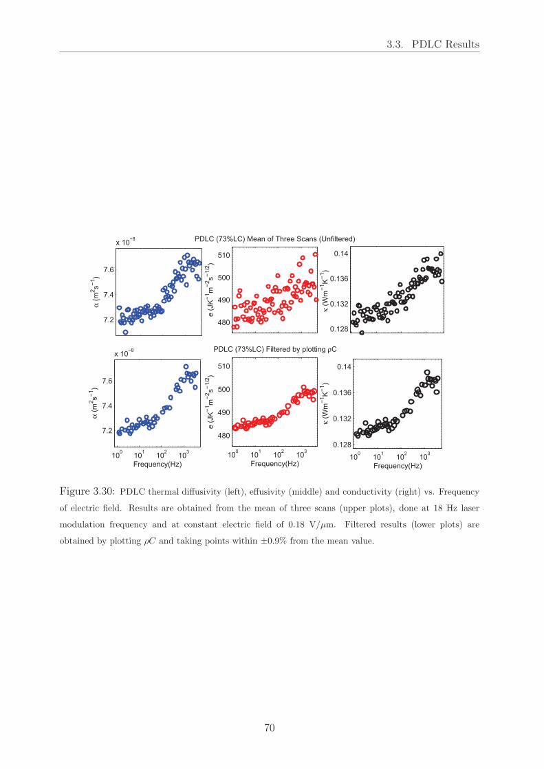
3.3. PDLC Results
0.128
0.132
0.136
0.14
κ (W
m−
1K
−1)
480
490
500
510
e (
JK
−1m
−2s
−1/2
)
PDLC (73%LC) Mean of Three Scans (Unfiltered)
7.2
7.4
7.6
x 10−8
α (
m2s
−1)
100
101
102
103
7.2
7.4
7.6
x 10−8
Frequency(Hz)
α (
m2s
−1)
100
101
102
103
480
490
500
510
Frequency(Hz)
e (
JK
−1m
−2s
−1/2
)
PDLC (73%LC) Filtered by plotting ρC
100
101
102
103
0.128
0.132
0.136
0.14
Frequency(Hz)
κ (W
m−
1K
−1)
Figure 3.30: PDLC thermal diffusivity (left), effusivity (middle) and conductivity (right) vs. Frequency
of electric field. Results are obtained from the mean of three scans (upper plots), done at 18 Hz laser
modulation frequency and at constant electric field of 0.18 V/µm. Filtered results (lower plots) are
obtained by plotting ρC and taking points within ±0.9% from the mean value.
70

3.3. PDLC Results
can estimate the mean thermal conductivity of LC droplets, given by:
κLC =κm [2κm (1− φ)− κPDLC (2 + φ)]
κPDLC [(1 + 2γ)− φ (1− γ)]− κm [1 + 2γ + 2φ (1− γ)](3.23)
Evolution of the mean thermal conductivity of LC droplets, κLC, for PDLC samples of
73%LC and 85% LC are shown in fig. 3.31. Calculations are done using the previously
obtained γ and φLC values from table 3.5.
100
101
102
103
0.2
0.21
0.22
0.23
0.24
0.25Mean Thermal Conductivity Evolution of LC Droplets
Frequency(Hz)
Therm
al conductivity (
W/m
/K)
85 wt% LC
73 wt% LC
Figure 3.31: Thermal conductivity of the confined liquid crystal as a function of frequency of the applied
electric field. Squares are showing the results on 85% LC and circles represents 73% LC.
Considering κLC⊥ and κLC‖ the thermal conductivity perpendicular to or along the
molecular long axis, and θ- the angle between this long axis and a given direction (fig.
3.32), the thermal conductivity along this direction may be express as:
κLC = κLC‖cos2θ + κLC⊥sin
2θ (3.24)
Using the values of κLC‖ and κLC⊥, the variation in orientation angle, θ, can be extracted
from the thermal conductivity experimental data:
θ = asin
√
κLC − κLC‖
κLC⊥ − κLC‖
(3.25)
Figures 3.33 and 3.34 are showing the variation of equilibrium angle of the directors,
θ, of LC droplets for both samples as a function of frequency of the applied electric field.
Evaluating the evolutions of θ in conjunction with the variations of κLC (fig. 3.31) reveal
71

3.3. PDLC Results
Figure 3.32: Orientation of LC droplets inside PDLC. θ is showing the average orientation of LC molecule
long axis with respect to the heat flow direction.
100
101
102
103
0
0.1
0.2
0.3
0.4
0.5
0.6
Mean Angle of LC Droplet Director (73% LC)
Frequency(Hz)
θ (r
adia
ns)
Figure 3.33: Angle (in radian) of the director with respect to heat flow direction as a function of
frequency of the applied electric field for 73% LC sample.
72

3.3. PDLC Results
100
101
102
0
0.1
0.2
0.3
0.4
0.5
Mean Angle of LC Droplet Director (85% LC)
Frequency(Hz)
θ (r
adia
ns)
Figure 3.34: Angle (in radian) of the director with respect to heat flow direction as a function of
frequency of the applied electric field for 85% LC sample.
the stamped down variations of thermal conductivity values in both samples.These fre-
quency behaviour of PDLC contains informations on several physical phenomenon. In the
subsequent sections, we have used the obtained results on θ and κLC for finding different
physical parameters.
3.3.5.3 Frequency Dependent Thermal Conductivity and MWS Effect
The relation between droplet electric field, Edrop, and the angle of molecular orientation,
θ, is given by[102] :
2cos2θ = 1 +e2 − 1 + 2cos2ψ
√
(e2 − 1)2 + 4e2cos2ψ(3.26)
where, ψ is the equilibrium angle of the droplet directors at zero electric field obtained
from EF varying experiments (values are displayed in table 3.6), e is the reduced field pa-
rameter and which can be expressed as: e = Edrop/E0 and E0 is the threshold reorientation
electric field. E0 can be defined as the electric field necessary to reorient LC molecules in
its direction (threshold electric field). Its value depends on the droplet radius (rd), elastic
constant (K) and the dielectric anisotropy (∆ǫ) of the LC material. ǫ0 is the permittivity
of free space (8.85×10⁻¹² F/m). The relation for E0 is given by [102]:
E0 ≈1
rd
√
K
ǫ0∆ǫ(3.27)
73

3.3. PDLC Results
In order to determine the effective thermal conductivity variations of PDLCs as a
function of frequency of the applied electric field, one can insert the equation for Edrop(fe)
(eq. (3.17)) into the equation for the angle of reorientation (θ, eq. (3.26)), the resultant
then put into the expression for LC droplet thermal conductivity (κLC, eq. (3.24)) and
finally to the expression for κPDLC(fe) (eq. (3.21)), as shown below:
Edrop(fe)Eq. (3.17)→ θ
Eq. (3.26)→ κLCEq. (3.24)→ κPDLC(fe)
The outcome of the above relation for κPDLC(fe) can be used to model the frequency
dependent effective thermal conductivity results of PDLC samples (figures 3.30 and 3.28)
to find electrical parameters of LC and polymer matrix as well as the threshold electric
field E0.
100
101
102
0.165
0.17
0.175
0.18
Frequency (Hz)
κ PD
LC
(W
/mK
)
PDLC (85% LC)
Figure 3.35: PDLC 85% LC experimental data (circle) and theoretical fit (full line).
Table 3.6: Electrical parameters of PDLC samples from MWS fit.
x ψ (rad.) σM (S/m) σLC (S/m) E0 (V/m) f0(Hz) Ea (V/m)
85% 0.6 (1.27±0.09)×10−9 (4.9±0.3)×10−8 (6.8±0.3)×104 21± 2 1.27×10⁵
73% 0.9 (3.5±0.1)×10−8 (4.8±0.1)×10−7 (7.2±0.1)×104 221± 5 1.80×10⁵
Figures 3.35 and 3.36 are showing the experimental results (circles) and the best fits
(full line) on effective thermal conductivity (κPDLC) variations of PDLC 85% LC and 73%
74

3.3. PDLC Results
101
102
103
0.13
0.132
0.134
0.136
0.138
Frequency (Hz)
κ PD
LC
(W
/mK
)
PDLC (73% LC)
Figure 3.36: PDLC 73% LC experimental data (circle) and theoretical fit (full line).
LC respectively as a function of frequency. The values of the EF were chosen from a
previous electric field scan (fig. 3.25) so that the LC molecules were aligned parallel to the
EF at a frequency high enough to nullify the MWS effects. During the fitting procedure,
E0 as well as electrical conductivities of both the polymer matrix and LC were kept as free
parameters. Values of the materials’ dielectric properties were taken from literatures. The
results obtained from fitting are displayed in table 3.6.
Figure 3.37 contains the simulated plots for 85% LC and 73% LC samples having the
values used in or obtained from the theoretical fitting of the experimental data. These
plots show the evolutions of Edrop and κPDLC for both samples. The threshold electric
fields (E0) and the corresponding frequencies (f0) are also labelled inside the plots and
also included in table 3.6. The electrical parameters for 85% LC found from fitting are in
good agreement with the values found in literatures (ref. section 3.3.2). While for 73%
LC sample, the results are showing relatively higher values than reported. One of the
reasons for this difference could be due to the possible variations in the solubility limit of
the LC. In addition, the system properties are vulnerable to change during the course of
time, temperature and synthesizing conditions.
The main interesting parameter in our study is the threshold field (E0)or frequency
(f0). These values are indicating the necessary field needed to align the LC molecules in
the direction of the applied EF. Obviously, the values of these parameters increase with
decreasing LC concentration. This behaviour is expected since the droplet size decreases
75

3.3. PDLC Results
100
101
102
103
0
5
10
15
fo ~ 221Eo ~ 7.197e+004
Frequency(Hz)
Edro
p (
×10
4 V
/m)
0
5
10
15
fo ~ 21Eo ~ 6.789e+004
Electric Field inside LC droplets and PDLC Thermal Conductivity
Edro
p (
×10
4 V
/m)
0.166
0.17
0.174
0.178
κP
DLC
85%
LC
(W
/mK
)
κPDLC
Edrop
100
101
102
103
0.13
0.134
0.138
κP
DLC
73%
LC
(W
/mK
)
κPDLC
Edrop
Figure 3.37: Simulations on Edrop and κPDLC with values used and obtained in fitting for PDLC 85%
LC (upper plot) and PDLC 73% LC (lower plot).
with decreasing concentration and thus the field across the droplet must be higher for
aligning the molecules. In the case of f0, the depolarisation field increases with decreasing
frequency thus the equivalent field acting on the droplets is linear to the applied frequency.
Table 3.7: Elastic constants for the PDLC samples.
x ∆ǫ rd(µm) E0 (V/m) K (N)
85% 10 0.5/2.5 (6.8±0.3)×104 9.4× 10⁻¹⁴/2.8× 10−12
73% 10 0.25/1 (7.2±0.1)×104 2.8× 10⁻¹⁴/4.7× 10−13
We can also deduce the elastic constant, K, knowing E0 and the droplet radius using eq.
(3.27). Values found for K for both of the PDLC samples are displayed in table 3.7. These
effective values of elastic constants govern the interaction between the anchoring forces
at the droplet-polymer boundaries, which make the droplet to be aligned in a particular
direction, and the elastic forces acting in the bulk of the LC droplet. The studied samples
are showing the values of K lower than that the value reported for bulk nematic 5CB
(4.1x10⁻¹²) [111]. This is attributed due to the increased anchoring forces at the LC-
polymer boundaries. Apparently, the K values are more closer and even similar for the
76

3.4. Summary of the Experimental Results on Liquid Samples
biggest droplets in the case of 85% LC to the reported bulk values, where the molecules
available away from the boundaries are higher than 73% LC sample.
3.4 Summary of the Experimental Results on Liquid
Samples
We have explored the ability of photothermal infrared radiometry for studying thermal
properties of liquid samples and demonstrated its capability to give results with high accu-
racy. The two presented configurations are described theoretically followed by experimental
results. BF-PTR gives the absolute thermal diffusivity of a sample knowing only the sam-
ple’s thickness and also the result is independent of the thermal parameters of surrounding
layers. B-PTR configuration has the potentiality of finding two thermal parameters simul-
taneously. Both the Back signal detection involved configurations, B-PTR and BF-PTR,
posses high sensitivity to the thermal parameters of the sample and can yield results from
a single modulation frequency. This is particularly helpful for finding thermal properties in
temperature or time varying experiments. We have done experiments with known samples
and found a very good agreement with already reported values of thermal parameters.
The newly developed PTR methods for thermal characterization of liquid samples are
used to investigate the variation of thermal transport properties due to the polarization
effects on PDLC samples. Results on thermal properties as a function of frequency depen-
dent electric field on PDLC samples are clearly showing the polarization field effects on
their thermal properties. These results are further analysed and modelled against existing
MWS model and deduced their elastic and electrical properties from the experimentally
found thermal informations.
77

Chapter 4
Thermal Characterization of
Thermoelectric Polymer-Nano
Composites using A Novel
Photothermoelectric (PTE)
Technique
4.1 Introduction
Certain materials produce an electrical potential difference when they are subjected to a
temperature gradient [112]. This phenomenon is called Seebeck effect and these solid-state
materials are called thermoelectric (TE) materials. Even though, at present, TE mate-
rials are less efficient than other energy harvesting systems like photovoltaic, they have
attracted the scientific community over the past decades [29]. New interests on TE mate-
rials started since the theoretical predictions suggested that the thermoelectric efficiency
could be strongly improved with nano-structuring [113, 114, 115, 116]. The performance
depends mainly on the dimensionless quantity called figure of merit ZT = S2σkT , where
S, σ, κ, T are the Seebeck coefficient, electrical conductivity, thermal conductivity and
the absolute temperature. Polymer thermoelectrics are new class of materials interestingly
emerged out after the finding of electrically conducting doped polyacetylene [117]. Since
78

4.2. A Novel PhotoThermoElectric Technique (PTE)
these materials are cost effective and easily processable than the conventional ‘state of
the art’ metal/semiconductor composite materials [118], a renewed interests on polymer
thermoelectrics arise to improve their efficiency.
Here, our experimental studies are focused on the investigation of thermal transport
properties of thermoelectric materials, in which, the characterisation of Polyaniline (PANI)
-Carbon Nanotube (CNT) nanohybrids, prepared using a novel approach called CNT-
templated polymerization process, are being analysed. Carbon nanotubes used for ex-
periments are either oxidized or unoxidized, single- or multiple-walled, and the as pre-
pared hybrids exhibit cable-like morphology with CNTs as cores, wrapped by nanofibrous
polyaniline (PANI) [22].
In this work, we introduce, for the first time, a novel application of the thermoelectric
effect as a means to investigate the thermal properties of both TE and other materials by
using TE materials as sensors. All the presented results, in this chapter, are obtained by
the newly developed photothermoelectric technique (PTE), where the samples themselves
serve as sensors. Results obtained from PTE measurements are then being compared with
those retrieved from conventional photothermal radiometry (PTR) as a validation of the
PTE technique.
Furthermore, we have used PTE technique for the thermal characterization of solid
samples. Here, the TE material as a PT sensor operate under two configurations: (i)
Front-PTE (FPTE), and (ii) Back-PTE (BPTE).
4.2 A Novel PhotoThermoElectric Technique (PTE)
The potential difference (∆V ) between two points of a thermoelectric material can be
described by the following relation provided that the temperature fluctuations are weak:
∆V = S
∫ Tz=0
Tz=d
dT (z ≤ 0) (4.1)
with, d is the thickness of the sample in the negative z-direction, Tz=0 and Tz=d are the
temperature at the surface z = 0 and at thickness z = d respectively. S is considered as
constant for small temperature variations. Figure (4.1) depicts the experimental configu-
ration. Upon integrating eq. (4.1) gives:
79

4.2. A Novel PhotoThermoElectric Technique (PTE)
∆V = S [T (z = 0)− T (z = d)] (4.2)
Referring back to the derived expressions in chapter 2 for the temperature fields for an
optically opaque sample of thickness d in contact with a semi-infinite substrate and air as
the top layer (layer-0 ), excited by a modulated laser beam is given by, including the terms
for convection heat transfer loss(H1) [119]:
T (z, ω) =I0(1 +H1)
4k1σ1
[
1 + ℜ2 exp(−2σ1(d+ z))
1−H1ℜ2 exp(−2σ1d)
]
exp(σ1z) (z ≤ 0) (4.3)
where I0, k1, ℜ2 and σ1 are intensity of the incident radiation, sample’s thermal conductiv-
ity, thermal wave reflection coefficient (eq. (2.42)) and the complex thermal wave number
(eq. (2.17)) respectively, as mentioned earlier.
Figure 4.1: Investigated sample configuration
H1 is a parameter depending on convec-
tion coefficient h1, followed by the relation:
H1 =k1σ1 − h1k1σ1 + h1
(4.4)
It should be pointed out that h1 can be
neglected for a given sample for high fre-
quency. In the following section 4.2.1 we
have carried out simulations to show the
suitable frequency range where h1 can be
neglected. By equating eq. (4.3) into eq. (4.2) and after rearranging, the potential differ-
ence between the two surfaces can be expressed as:
∆V =SI0(1 +H1)
4k1σ1
[
1 + ℜ2 exp(−2σ1d)− (1 + ℜ2) exp(−σ1d)1−H1ℜ2 exp(−2σ1d)
]
(4.5)
The normalized signal is obtained by realising frequency scans with separate substrates,
e.g., air and glycerol. When the substrate is air, ℜ2 becomes ℜ0 (eq. (2.42)) and the
voltage difference is given by:
∆V0 =SIo(1 +H1)
4k1σ1
[
1 + ℜ0 exp(−2σ1d)− (1 + ℜ0) exp(−σ1d)1−H1ℜ0 exp(−2σ1d)
]
(4.6)
Further, considering that the thermal transport by conduction largely outweighs the ther-
mal transport by convection, the real part of k1σ1 ≫ h1, then the quantity H1 can be
80

4.2. A Novel PhotoThermoElectric Technique (PTE)
approximated to 1 and also, since the air effusivity is too low ℜ0 ≈ 1. Then the normalized
voltage Vn, obtained by dividing ∆V with ∆V0 is given by, after simplification:
Vn =∆V
∆V0= 1 +
(1−ℜ2) exp(−σ1d)1−ℜ2 exp(−2σ1d)
. (4.7)
Apparently, the phase (normalized phase) from eq. (4.7) decreases with frequency and
becomes zero for a first time at a value d/µ1 = π. Thus, the thermal diffusivity of the
sample, α1, can be extracted from, as previously reported for photopyroelectric techniques
[120]:
α1 =d2f0π
, (4.8)
where, f0 is the zero crossing frequency. Knowing α1, the thermal effusivity can be
obtained after some rearrangements of eq. (4.7):
e1 = e21 + ℜ2
1−ℜ2
. (4.9)
where, ℜ2 is given by:
ℜ2 =(Vn − 1)− exp(−σ1d)
(Vn − 1) exp(−2σ1d)− exp(−σ1d). (4.10)
Therefore, both thermal parameters of the TE sample (as sensor) can be determined either
by a direct least squares fitting of eq. (4.7) to experimental data or analytically using eqs.
(4.8), (4.9) and (4.10) provided that the effusivity of backing is known.
4.2.1 Simulations on Convection Effects and Sensitivity
Due to the poor thermal conductivity of polymers, the measurements need to be carried
out at lower frequencies, meaning that convection effects can not be neglected. In order to
take into account of this phenomenon, the influence of the convection effect on the PTE
signal is investigated numerically.
Figure 4.2 shows the evolution of the normalized phase vs. reduced parameter d/µ1,
where µ1 is the thermal diffusion length. h1 is varied for values 0, 10 and 100 Wm−2K−1
keeping ℜ2 fixed at -0.2. It is apparent that, above d/µ1 = 1, convection has little or no
effect on the normalized signal, thus the eq. (4.7) without convection factor is valid for
81

4.2. A Novel PhotoThermoElectric Technique (PTE)
0.2
0.4
0.6
0.8
1
Norm
aliz
ed A
mplit
ude
h = 0
h = 10 Wm−2
K−1
h = 100 Wm−2
K−1
10−1
100
101
0
10
20
30
Norm
aliz
ed p
hase (
°)
d/µ1
Figure 4.2: Dependence of normalized signal evolution vs. reduced thermal parameter d/µ1 for different
values of convection coefficient plotted with fixed ℜ2=-0.2. Upper plot showing the normalized amplitude
and lower one is the phase difference
d/µ1 ≥ 1. For d/µ1 < 1, convection cannot be neglected and the equation including H
must be used.
Figures 4.3 -(a & b) are showing the sensitivity of experimental signal vs. d/µ1 for
various values of ℜ2 for a 1% change in thermal diffusivity. The sensitivity increases with
decreasing ℜ2 value, indicating that a substrate with high effusivity need to be used for
the determination of the thermal diffusivity. While in the case of sensitivity studies on
effusivity variations, the best frequency range found is 0.5 ≤ d/µ1 ≤ 2 (fig. 4.3 -(c &
d) plotted with 1% change in e1 around each ℜ2 values keeping zero percentage change
in α1). However, in order to avoid convection during experiments, the frequency scans
are restricted to d/µ1 ≥ 1, limiting the available frequency range to 1 ≤ d/µ1 ≤ 2. As
expected, sensitivity on thermal effusivity increases when the thermal effusivity contrast
increases, means ℜ2 goes far from 0.
4.2.2 Experimental Results using PTE technique
4.2.2.1 Intrinsically Conducting Polymers
Polymer composite materials identifies as an indispensable stuff in our scientific arena. It
creates a new distinguished class of material, which are light in weight and mechanically
stronger in utility. The ease of preparation and possibility of reprocessing opens cost effec-
tive solutions for many applications using polymer composites. Polymers were previously
82

4.2. A Novel PhotoThermoElectric Technique (PTE)
0 1 2 3 4 5 6 7
−0.15
−0.1
−0.05
0
0.05
0.1
d/µ1
−0.2
0
0.2
0.4Sensitivity Studies on Diffusivity
ℜ2=0.5
ℜ2= 0
ℜ2=−0.5
0 1 2 3 4 5 6
−0.05
0
0.05
d/µ1
−0.2
−0.1
0
0.1
0.2Sensitivity Studies on Effusivity
ℜ2 = 0.5
ℜ2 = 0.2
ℜ2= −0.2
ℜ2 = −0.5
d)
c)
a)
b)
Figure 4.3: Simulations for the variation of normalized amplitude in percentage (a & c) and phase
difference in degree (b & d) vs. d/µ1 for various ℜ2 values. In a & b the thermal diffusivity (α1) is
varied 1% for all the plots. For c & d, 1% change in e1 is introduced around each ℜ2 values while keeping
0% change in α1. Values used for simulations are: α1 = 3.2 × 10⁻⁷ m2s−1, e1 = 1184 Jm−2K−1s−1/2,
d =200µm and e2 = 1581 Jm−2K−1s−1/2
known as electrically insulting materials until the recent findings of appreciable electrical
conductivity in them. This circumstantial findings lead to the developments on using such
intrinsically conducting polymers (ICPs) as bio-materials [121], actuators [122], fabrics
[123], corrosion inhibitors [124], in electronics [125], organic LEDs and PVs, charge dissi-
pating (antistatic) layers and chemical sensor research. ICPs are polymers with extended
π-conjugation along the molecular backbone. Their conductivity can be changed by several
orders of magnitude from a semiconducting state to a metallic state by doping. Usually
p-doping is achieved by partial oxidation of the polymer by a chemical oxidant or an elec-
trochemical method, and causes depopulation of the bonding π orbital (HOMO) with the
formation of “holes” [126]. The possibility of generating electricity [3, 127, 128] due to
its thermoelectric (TE) properties, based on the Seebeck effect (property of a material
to generate a potential difference between the ends when it is subjected to a tempera-
ture difference at those ends), is also a live research area. The conversion efficiency of
thermo-electricity generation is governed by the dimensionless quantity known as figure of
merit, ZT = S2σT/κ. Here S, σ, T and κ are the Seebeck coefficient(V/K), electrical con-
ductivity(S/m), absolute temperature(K) and thermal conductivity(W/mK) respectively.
Until now, metallic or semi-metallic composites are showing the best ZT and the highest
83

4.2. A Novel PhotoThermoElectric Technique (PTE)
reported value is about 2.2 [129] at around 9000C. Even though these ZT values are far be-
low in comparison with the equivalent efficiency of compressor type cooling systems. This
restricts the use of TE materials from efficient application oriented implementations. The
class of polymer thermoelectrics have even lower ZT values, typically < 1. Even though,
a significant interest on TE research stems on the solid state and cost effective energy
conversion possibility and waste heat recovery advantages. Thus many of the researchers
are being focused on improving the ZT values of both types (polymer and metallic) of
TE materials by hoping on different theoretical predictions and possibilities such as nano
structuring, doping etc. to increase S, σ and/or to decrease κ. Recent studies on conduct-
ing polymers have shown improved ZT values on the tailor-made polymer nano-composites
than pure polymers. These composites exhibit high electrical conductivities, depending on
the amount of nano inclusions, without a major increase in thermal conductivity.
4.2.2.2 Sample Preparation
The TE samples are pressed pellets (diameter: 13 mm) of Methanesulfonic acid (CH3SO3H)
doped nanofibrous Polyaniline (PANI) used as sheath to wrap CNT core yielding nanos-
tructured composite materials (Fig. 4.1). The Carbon Nanotubes (CNT) mass fraction is
≈ 6.6 wt-%. Four composites are investigated: PANI-CH3SO3H/unoxidized Single-Walled
Carbon Nanotubes (PANI/unoxSWNT), PANI-CH3SO3H/unoxidized Multi-Walled Car-
bon Nanotubes (PANI/unoxMWNT), PANI-CH3SO3H/oxidized SWNT (PANI/oxSWNT)
and PANI-CH3SO3H/oxidized MWNT (PANI/oxMWNT). Details of sample pellet process-
ing are described elsewhere [22]. Each surface of the pellets were covered with a sputtered
silver electrode on which electrical leads were silver pasted and plugged into an EG&G
7260 lock-in amplifier (Fig. 4.1). Figure 4.4 shows the SEM images of each samples of
polyaniline-CNT nano hybrides. These images are confirming that the in situ polymeriza-
tion of aniline has been taken place and as grown PANI-CNTs evidently forming fibrous
hybrids with a minimum size bigger than the smallest nanotube diametrically. The longer
lengths of all the hybrid nano fibres (fig. 4.4 b,c,d,e) than the pristine PANI fibres (fig.
4.4 a) are also justifying the guided growth of PANI along the CNT backbone.
84

4.2. A Novel PhotoThermoElectric Technique (PTE)
Figure 4.4: SEM images of CH3SO3H doped-PANI/CNT nanohybrids: (a) PANI, (b)
PANI/UnOxSWNT, (c) PANI/OxSWNT, (d) PANI/UnOxMWNT, and (e) PANI/OxMWNT.
4.2.2.3 Experimental Details
Conducting experiments based on PTE technique are more or less similar to the phototpy-
roelectric (PPE) experiments [42, 130]. For PTE, the sensor is a thermoelectric (TE) device
rather than a pyroelectric generator as in PPE. For making sensors all the PANI-CNT pel-
lets were coated on both sides with gold or silver using a sputter coater (Cressington 108)
or silver painted and attached electrical contacts on both sides. The electrically conducting
coatings integrate all the generated charges on both surfaces of the sensor. A lock-in ampli-
fier in voltage mode, connected directly to the PTE sensor, was used to detect the signal.
We have used pure PANI samples and also composites with carbon nanotubes (CNT) as
sensors. Typical electrical resistance between the terminals of the sensor measured was
only a few ohms. The laser power used was also comparatively high (∼ 750 mW) in order
to get enough signal. Typically the signal was around 10 µV at a modulation frequency
of 2 Hz and the noise level was as low as 50 nV. The laser power was chosen so that the
signal to noise ratio stays better than 10 in the highest modulation frequency used for the
experiment.
85

4.2. A Novel PhotoThermoElectric Technique (PTE)
4.2.2.4 Results and Discussion
0
5
10
15
Am
plit
ude (
µV)
Experimental signal before Normalizaton (OxSWNT−PANI)
100
101
102
103
120
140
160
180
200
Phase(°
)
Frequency (Hz)
glycerol substrate
air substrate
glycerol substrate
air substrate
Figure 4.5: Experimental Signals obtained from PANI-OxSWNT using air and glycerol as backings.
Amplitude (upper plot) and Phase (lower plot).
Experiments have been carried out using the setup described in Fig. 4.1. A typi-
cal Amplitude and phase data of a photothermoelectric (PTE) experimental signal for a
348.5µm thick doped PANI-OxSWNT are presented in fig.4.5 using either air or glycerol
as substrates. Though the measured voltages for the signal amplitudes were weak (≤ 10
µV), it can still be exploited with a satisfactory signal to noise ratio. Amplitude ratios
and phase differences for the OxSWNT-PANI signals in fig. 4.5 are calculated and de-
picted as in fig.4.6. Thermal parameters are retrieved by fitting the signal against eq.(4.7)
while considering h1 = 0 ; the thermal diffusivity of α1 = (4.68 ± 0.04)×10−7 m2s−1 and
a thermal effusivity of e1 = (1212 ± 25) Ws1/2m−2K−1 are obtained. Then the thermal
conductivity was calculated using the relationship k1 = e1√α1 and the result is k1 = (0.83
± 0.02) Wm−1K−1.
These results for OxSWNT-PANI sample were also calculated analytically using the
zero crossing frequency (f0 = 11.5 Hz) of the normalized phase using eq. (4.8). It led to a
thermal diffusivity value of (4.45 ± 0.10)×10−7 m2s−1. Based on this value, thermal effu-
sivity has also been calculated from eq. (4.10) and obtained, e = 1212± 37 Ws1/2m−2K−1
and the corresponding thermal conductivity value is 0.81± 0.04 Wm−1K−1.
86

4.2. A Novel PhotoThermoElectric Technique (PTE)
0.8
0.9
1
1.1
1.2N
orm
aliz
ed a
mplit
ude
PTE normalized signal (OxSWNT−PANI)
100
101
102
103
−15
−10
−5
0
5
Norm
aliz
ed p
hase (
°)
Frequency (Hz)
Full experimental data
FItted data
Fit
Figure 4.6: Normalized amplitude (upper plot) and phase (lower plot) from PTE experiment on
OxSWNT-PANI
Table 4.1: Thermal parameters retrieved using PTE techniques for the PANI-OxSWNT composite; α:
thermal diffusivity; e: thermal effusivity, k: thermal conductivity.
ParameterPTE PTE
(fit) (analytic)
Diffusivity (× 10−7 m2/s) 4.68± 0.04 4.45± 0.10
Effusivity (J/Km2s1/2) 1212 ± 25 1212 ± 37
Conductivity (W/mK) 0.83 ± 0.02 0.81 ± 0.04
87

4.3. Photothermal Radiometry Experiments as a Validation for PTE Results
4.3 Photothermal Radiometry Experiments as a Val-
idation for PTE Results
Conducting measurements on solid samples using PTR are well established and extensively
using for the accurate determination of thermal parameters [82, 131, 132]. The method
for simultaneous determination of thermal diffusivity and effusivity of free standing thin
layers is of interest [133]. Theoretical model for our experiments considers a three layer
configuration with air as the top layer (layer-0 ), the sample as layer-1 and air or liquid
with well known thermal parameters as the backing (layer-2 ), depicted as in fig. 2.2.
The sample is considered as optically opaque and the backing is thermally semi infinite.
Using the surface absorption model described by eq. (2.41), at z = 0, can be used to
find the temperature field at the sample surface and it reveals the thermal parameters of
the sample. The reference signal for the normalisation can be obtained by performing the
experiment with another backing material (e.g., air replaced with water) without altering
the sample and layer-1. This means ℜ2, in eq. (2.41), is the only modifying parameter.
Thus the equation for the normalised signal obtained by dividing two frequency scans with
two different backing materials can be written as:
ΓF (ω, z = 0) =I0
2σ1k1(1 + b01)
(
1 + ℜ2e−2σ1d
1−ℜ0ℜ2e−2σ1d
)
× 2σ1k1(1 + b01)
I0
(
1−ℜ0ℜ2re−2σ1d
1 + ℜ2re−2σ1d
)
(4.11)
where, ℜ2 is replaced by ℜ2r in the reference (normalization) signal.
Approximation while using ‘air’ interfaces:- Because of the extremely low effusivity
of air medium makes the effusivity ratios b01 and b21 at both the sample interfaces will
become negligibly small. The approximated terms are:
b01 ≈ 0, b21 ≈ 0, ℜ0 ≈ 1, ℜ2 ≈ 1
So the eq. (4.11) can be rearranged and rewritten as:
ΓF (ω, z = 0) =
(
1 + e−2σ1d
1− e−2σ1d
)(
1−ℜ2re−2σ1d
1 + ℜ2re−2σ1d
)
(4.12)
Multiplying the terms in the above eq. (4.12) and neglecting the higher order exponen-
tial term(
e−4σ1d)
, which has again negligible contribution, will result in:
ΓF (ω, z = 0) =1 + (ℜ2r − 1)e−2σ1d
1− (ℜ2r − 1)e−2σ1d(4.13)
88
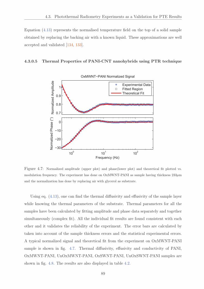
4.3. Photothermal Radiometry Experiments as a Validation for PTE Results
Equation (4.13) represents the normalised temperature field on the top of a solid sample
obtained by replacing the backing air with a known liquid. These approximations are well
accepted and validated [134, 133].
4.3.0.5 Thermal Properties of PANI-CNT nanohybrids using PTR technique
0.7
0.8
0.9
1
Norm
aliz
ed A
mplit
ude
OxMWNT−PANI Normalized Signal
100
101
102
−30
−20
−10
0
Frequency (Hz)
Norm
aliz
ed P
hase (
°)
Experimental Data
Fitted Region
Theoretical Fit
Figure 4.7: Normalized amplitude (upper plot) and phase(lower plot) and theoretical fit plotted vs.
modulation frequency. The experiment has done on OxMWNT-PANI as sample having thickness 233µm
and the normalization has done by replacing air with glycerol as substrate.
Using eq. (4.13), one can find the thermal diffusivity and effusivity of the sample layer
while knowing the thermal parameters of the substrate. Thermal parameters for all the
samples have been calculated by fitting amplitude and phase data separately and together
simultaneously (complex fit). All the individual fit results are found consistent with each
other and it validates the reliability of the experiment. The error bars are calculated by
taken into account of the sample thickness errors and the statistical experimental errors.
A typical normalized signal and theoretical fit from the experiment on OxMWNT-PANI
sample is shown in fig. 4.7. Thermal diffusivity, effusivity and conductivity of PANI,
OxMWNT-PANI, UnOxMWNT-PANI, OxSWNT-PANI, UnOxSWNT-PANI samples are
shown in fig. 4.8. The results are also displayed in table 4.2.
89

4.3. Photothermal Radiometry Experiments as a Validation for PTE Results
0
0.4
0.8
1.2
1.6
2
2.4Themal Paramaters of PANI−CNT Composites
PANI
OxMW
NT−PANI
UnOxMW
NT−PANI
OxSW
NT−PANI
UnOxSW
NT−PANI
κ(W
/mK
);e [
×10
3 (
JK
−1m
−2s
−1/2
)]
0
2
4
x 10−7
α (
m2s
−1)
Conductivity
Effusivity
Diffusivity
Figure 4.8: Thermal parameters with error bar of different PANI-CNT composites measured using PTR
technique. The results are also displayed in table 4.2.
Table 4.2: Thermal diffusivity, effusivity and conductivity results of PANI-CNT samples (PTR results).
PANI- Thermal diffusivity Thermal effusivity Thermal conductivity
composite ×10−7 α (m2s−1) e (JK−1m−2s−1/2) κ (Wm−1K−1)
PANI 1.44±0.06 1132±133 0.43 ±0.01
-OxMWNT 2.87±0.01 1084±10 0.581±0.002
-UnOxMWNT 2.89±0.02 1293±21 0.695±0.001
-OxSWNT 4.3±0.1 1292±72 0.850±0.007
-UnOxSWNT 4.38±0.07 1523±53 1.01 ±0.004
90

4.4. Results and Discussions on Thermoelectric Properties of PANI-CNT nanohybrids
4.4 Results and Discussions on Thermoelectric Prop-
erties of PANI-CNT nanohybrids
All the PANI-CNT samples were experimentally investigated using PTE technique and val-
idated the results by conducting PTR experiments. A complete set of results on thermal
diffusivities, effusivities and conductivities of all PANI composites measured using both
PTE and PTR techniques are presented in table 4.3. Figure 4.9 is the graphical repre-
sentation of the results using PTE technique alone. The results are clearly showing that
the SWNT based composites exhibit higher thermal diffusivities and thermal conductivi-
ties than their MWNT counterparts. Evidently, UnOxSWNT-PANI showing the highest
thermal conductivity with an increase of around 2.5 times than pure PANI. The lower
conductivity values of MWNT composites than the SWNT composites are attributed to
the usual higher thermal conduction property of SWNTs. Among all the four composites,
oxidized nanotube composites are showing a little lower thermal conductivity values than
their un-oxidized counter parts. This might be due to the presence of oxide layer along the
surface of the nanotubes, which, upto a small extend, hindering the heat transport at the
matrix-nanotube boundaries. Electrical conductivity studies on this same set of samples
[22] are also confirming the same trend as from our thermal studies. Of interest, it is also
pointing out that, regardless of the nature of the inclusions, the thermal effusivities stay
roughly constant, which indicate the thermal conductivity behaviour is mainly controlled
by the thermal diffusivity. Here, the higher thermal conductivities of individual SWNTs in
comparison with individual MWNTs attributed to the higher thermal conductivity values
of SWNT-PANI composites. Although it is acknowledged that SWNTs present a higher
interfacial thermal resistance than the MWNTs [135], this property, however, is not suffi-
cient to mitigate the effects of thermal conductivity differences between the aforementioned
tubes. We believe, this is due to the strong polymer-nanotube interaction that came from
the in situ polymerization procedure. Further, the thermal conductivities of oxidized nan-
otubes based composites are lower than their unoxidised counterparts. This behaviour can
be explained by the oxidation process of CNTs which induces defects on the nanotubes.
These defects scatter the phonons, and, thus, lower the thermal conductivity. A similar
behaviour has been suggested for the lowering of the electrical conductivity in the case of
oxidized CNT due to induced carrier scattering centres.
91

4.4. Results and Discussions on Thermoelectric Properties of PANI-CNT nanohybrids
Table 4.3: Thermal diffusivity, effusivity and thermal conductivity Results of PANI-CNT samples.
PANI-Thermal diffusivity Thermal effusivity Thermal conductivity
×10−7 α (m2/s) e (J/Km2s1/2) κ (W/mK)
PTR PTE PTR PTE PTR PTE
PANI 1.44±0.06 1.2±0.05 1132±133 1129±103 0.43 ±0.01 0.39±0.01
-OxMWNT 2.87±0.01 2.94±0.02 1084±10 1070±25 0.581±0.002 0.58±0.01
-UnOxMWNT 2.89±0.02 2.8±0.2 1293±21 1402±191 0.695±0.001 0.74±0.03
-OxSWNT 4.3±0.1 4.68±0.04 1292±72 1212±25 0.850±0.007 0.83±0.02
-UnOxSWNT 4.38±0.07 4.87±0.08 1523±53 1316±40 1.01 ±0.004 0.92±0.01
0
1
2
3
4
5x 10
−7
α (
m2s
−1)
Thermal Parameters of PANI−CNT Composites (PTE)
0
500
1000
1500
e (J
K−
1m
−2s
−1/2
)
0
0.2
0.4
0.6
0.8
1
κ (W
/mK
)
PANI
OxMWNT P
ANI
UnoxMWNT P
ANI
OxSWNT P
ANI
UnoxSWNT P
ANI
Figure 4.9: Experimental results of thermal parameters for PANI-CNT composites (PTE results)
92

4.4. Results and Discussions on Thermoelectric Properties of PANI-CNT nanohybrids
Table 4.4 shows the Seebeck coefficient, electrical conductivity and thermal conductivi-
ties values obtained for various composites. Figure of merit (ZT ) for each material samples
have been calculated from these parameters using the formula ZT = S2κe
kT , at ambient
temperature (T = 300K). The results are displayed in figure 4.10. It is obvious from the fig-
ure that the ZT is considerably enhanced with the incorporation of carbon nanotubes into
the polymer material even with a small fraction of CNT (6.6 wt-%). Overall, nanocompos-
ites containing unoxidized and single-walled CNTs exhibit better thermophysical properties
than their oxidized or multiple-walled counterparts.
Table 4.4: Seebeck coefficient, electrical conductivity and thermal conductivity Results.
MaterialSeebeck Coefficient Electrical Conductivity Thermal Conductivity
S (µV/K) κe (S/m) κ (W/mK)
PANI 5.8 0.82 0.39±0.01
PANI-OxMWNT 13.5 14 0.58±0.01
PANI-UnOxMWNT 10.6 70.1 0.74 ±0.03
PANI-OxSWNT 12 132.23 0.83±0.02
PANI-UnOxSWNT 33 530.98 0.92±0.004
1e−8
1e−6
1e−4
ZT
Figure of Merit for the PANi−CNT Composites
PANI
OxMWNT P
ANI
UnoxMWNT P
ANI
OxSWNT P
ANI
UnoxSWNT P
ANI
Figure 4.10: Figure of Merit for the PANI-CNT composites
Clearly, a careful choice of CNTs and their blending with traditional intrinsically con-
ducting polymers have led to an enhancement of the hybrid Seebeck coefficient and electri-
93

4.4. Results and Discussions on Thermoelectric Properties of PANI-CNT nanohybrids
cal conductivity without increasing significantly their thermal conductivity due to interfa-
cial thermal resistances between the nanotubes and the polymeric matrix. These improve-
ments contribute nearly four orders of magnitude increase in ZT value in the unoxidized,
single-walled hybrid sample. However, its ZT value of 2 × 10⁻⁴ remains low and is far
from reaching the recommended 2 - 3 ZT range required for a technological breakthrough.
Nevertheless, the present work has its advantages because of the preparation methods and
sample processing are inexpensive and straightforward. There are also possibilities for fur-
ther improvements in hybrid physical characteristics by a judicial choice/amount of each
constituent of the hybrid and their synthesize.
4.4.0.6 Summary of the results on PANI-CNT samples
We have reported a new photothermal experiment for the determination of thermal prop-
erties based on PhotoThermoElectric (PTE) effect. It has been demonstrated that pa-
rameters such as thermal diffusivity, effusivity and conductivity of a nano-structured ther-
moelectric material can be determined analytically and numerically using PTE technique.
The main advantage of this approach permits the assessment of the thermal properties of
a TE material without the need of an external sensor. The formalism of the PTE signal
has been developed and numerical as well as analytical procedures for extracting thermal
parameters are also proposed. The thermal parameters retrieved from the PTE signals
for PANI-CNT samples have been compared with those obtained from the conventional
Photothermal Radiometry experiment. A good agreement has been found between the
two different experimental techniques demonstrating the relevance and the usefulness of
the developed methodology. It is also noteworthy that the values obtained for the thermal
conductivity from the analytical procedure were similar to the results obtained from the fit-
ting procedure with an agreement better than 97 %. Therefore, the proposed methodology
provides an accurate and simple way to determine the thermal conductivity of TE materials
without any intermediate media which makes this technique full of prospects. Using this
novel technique, various doped PANI/(oxidized or unoxidized, single or multiple-walled)
CNT composites have been investigated and thermal parameters were deduced. Know-
ing the Seebeck coefficient and electrical conductivity values, ZT have been calculated.
Among the investigated samples, PANI/unoxidized SWNT nano-composite showed the
most promising TE characteristics. This result can be explained by i) the electrical con-
94

4.5. PTE Technique for Thermal Investigation of Solids samples
ductivity improvement provided by the high SWNT electrical conductivity ,and, ii) the
weak thermal conductivity increase resulting from interfacial thermal resistances between
nanotubes and PANI. The CNT oxidization process creates defects on the nanotubes lead-
ing to a decrease of the thermal conductivity.
4.5 PTE Technique for Thermal Investigation of
Solids samples
TE materials can also be used as temperature sensors for the characterization of materials
thermally. Similar to the PPE methods, the detection configurations can be classified as:
(i) the “front” one (sensor directly irradiated and sample in back position) coupled with
TWRC method (scan of the liquid’s thickness), for thermal effusivity measurements [136,
137, 79] and (ii) the “back” one (sample directly irradiated and sensor in back position),
together with the chopping frequency scan, for thermal diffusivity investigations [138].
Further we are deriving the equations for these two configurations, so called Front-PTE
(FPTE) and Back-PTE (BPTE).
4.5.1 Front Photothermoelectric Configuration (FPTE)
Theoretical model for the FPTE configuration is depicted as in figure 4.11. Here the model
has to accommodate one more layer than we have derived in the previous chapter. Since the
basic procedure for any number of layers are same, we are expanding the already derived
three layer model with extra terms in order to obtain a theoretical model for a four layer
configuration. A proposed solution for the temperature field T3 for an additional fourth
layer can be written as:
T3 =(
A3eσ3z +B3e
−σ3z)
eiωt [z ≤ −(d+ b)] (4.14)
where, d and b are the thickness of layer: 2 and layer: 3. A3 and B3 are the unknown
constants. The boundary conditions for solving the equation are:
κ2∂T2∂t
= κ3∂T3∂t
, T2 =T3, [z = −(d+ b)] (4.15)
95
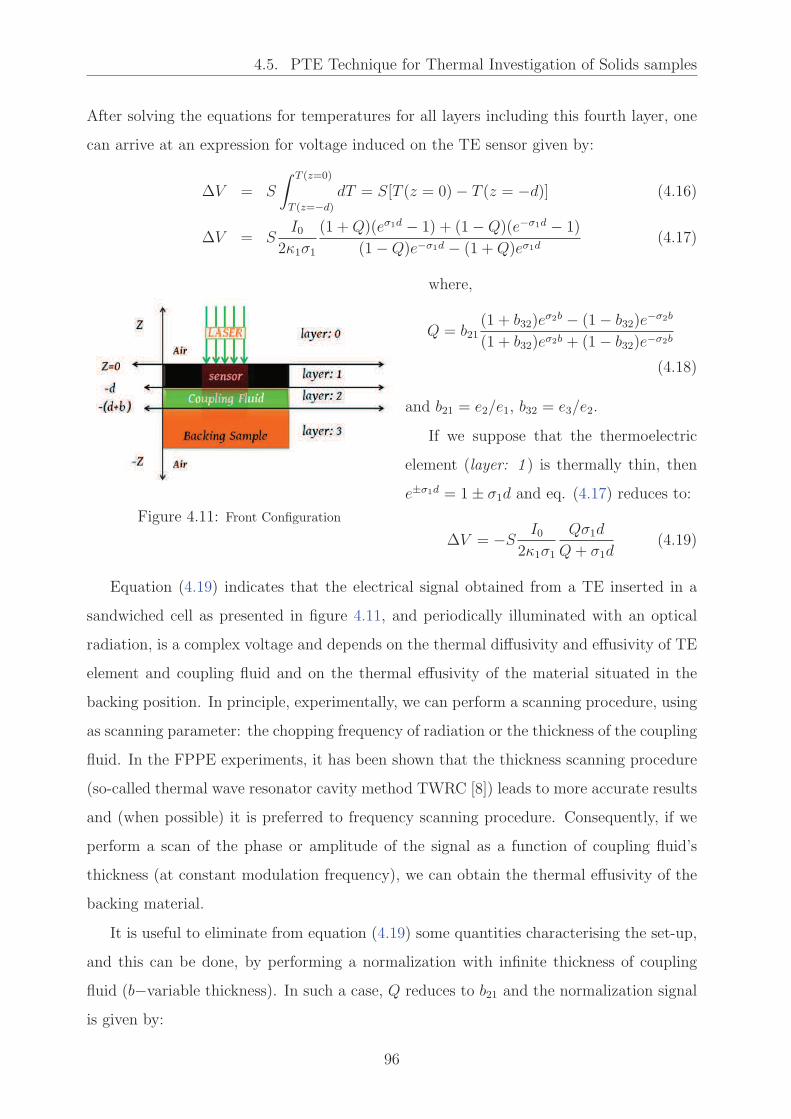
4.5. PTE Technique for Thermal Investigation of Solids samples
After solving the equations for temperatures for all layers including this fourth layer, one
can arrive at an expression for voltage induced on the TE sensor given by:
∆V = S
∫ T (z=0)
T (z=−d)
dT = S[T (z = 0)− T (z = −d)] (4.16)
∆V = SI0
2κ1σ1
(1 +Q)(eσ1d − 1) + (1−Q)(e−σ1d − 1)
(1−Q)e−σ1d − (1 +Q)eσ1d(4.17)
Figure 4.11: Front Configuration
where,
Q = b21(1 + b32)e
σ2b − (1− b32)e−σ2b
(1 + b32)eσ2b + (1− b32)e−σ2b
(4.18)
and b21 = e2/e1, b32 = e3/e2.
If we suppose that the thermoelectric
element (layer: 1 ) is thermally thin, then
e±σ1d = 1± σ1d and eq. (4.17) reduces to:
∆V = −S I02κ1σ1
Qσ1d
Q+ σ1d(4.19)
Equation (4.19) indicates that the electrical signal obtained from a TE inserted in a
sandwiched cell as presented in figure 4.11, and periodically illuminated with an optical
radiation, is a complex voltage and depends on the thermal diffusivity and effusivity of TE
element and coupling fluid and on the thermal effusivity of the material situated in the
backing position. In principle, experimentally, we can perform a scanning procedure, using
as scanning parameter: the chopping frequency of radiation or the thickness of the coupling
fluid. In the FPPE experiments, it has been shown that the thickness scanning procedure
(so-called thermal wave resonator cavity method TWRC [8]) leads to more accurate results
and (when possible) it is preferred to frequency scanning procedure. Consequently, if we
perform a scan of the phase or amplitude of the signal as a function of coupling fluid’s
thickness (at constant modulation frequency), we can obtain the thermal effusivity of the
backing material.
It is useful to eliminate from equation (4.19) some quantities characterising the set-up,
and this can be done, by performing a normalization with infinite thickness of coupling
fluid (b−variable thickness). In such a case, Q reduces to b21 and the normalization signal
is given by:
96

4.5. PTE Technique for Thermal Investigation of Solids samples
∆V0 = − SI02κ1σ1
b21σ1d
(σ1d+ b21)(4.20)
The normalized voltage becomes,
∆Vn =∆V
∆V0=
[σ1d+ b21][
(1 + b32) eσ2b − (1− b32) e
−σ2b]
(1 + b32) eσ2b (σ1d+ b21) + (1− b32) e−σ2b (σ1d− b21)(4.21)
4.5.2 Back Photothermoelectric Configuration (BPTE)
Figure 4.12: Front Configuration. Opaque sample and
thermoelectric sensor
The 2-layers detection cell in back con-
figuration is shown schematically in fig-
ure 4.12.
In this configuration, the opaque
front surface of the sample is irradi-
ated, and the heat is generated at the
gas-sample interface. Thermal diffu-
sion equations together with boundary
conditions are the same. So the equa-
tion for the voltage generation in the
TE sensor can be written as, according
to figure 4.12,
∆V = S
∫ T (z=−d)
T (z=−d−b)
dT
= S[T (z = −d)− T (z = −d− b)] (4.22)
If we impose from the beginning the condition of thermally thick sensor we can approx-
imate e−σ2b ≈ 0, and applying the boundary conditions, we get the following expression
for the PTE signal:
∆V =SI0
κ2σ2 [(b12 − 1)e−σ1d − (b12 + 1) eσ1d](4.23)
The easiest way to normalize the signal described by eq. 4.23 is to perform a measurement
with empty sensor. If d = 0, the normalization signal becomes:
∆V0 = − SI02κ2σ2
(4.24)
97

4.5. PTE Technique for Thermal Investigation of Solids samples
and the normalized one:
∆Vn =2 exp(−σ1d)
(b12 + 1)− (b12 − 1) exp(−2σ1d)(4.25)
If, additionally, the sample is at quasi thermally thick frequency regime then e−2σ1d ≈ 0
and eq. (4.25) reduces to:
∆Vn =2e−σ1d
(b12 + 1)(4.26)
Equation 4.26 indicates that a similar scan of the phase of the BPTE signal as a function
of the chopping frequency (at constant thickness), or thickness of the layer 1 (for liquid
samples, at constant frequency) can lead to the direct measurement of sample’s thermal
diffusivity. The amplitude can also be used for thermal effusivity measurement.
4.5.3 Comparison with PPE
When using the photopyroelctric (PPE) technique, in the same FPPE configuration and
approximation (thermally thin sensor and coupling fluid), the normalized FPPE voltage is
given by [139]:
V FPPEn =
σ1d+ b21
(σ1d) + b21
[
1+ℜ32e−2σ2b
1−ℜ32e−2σ2b
] (4.27)
with ℜ32 = (b32 − 1)/(b32 + 1) which is practically identical with eq. (4.21). When work-
ing with PPE, in the back (BPPE) configuration, in the thermally thick regime for the
pyroelectric sensor we obtain:
V BPPEn =
2
(b12 + 1)e−σ1d (4.28)
which is different from eq. (4.25), but in the thermally thick limit for the sample, the two
detection configurations lead to the same result.
4.5.4 Mathematical simulations
As pointed out before [140], when it is possible, we use as source of information only
the phase of the signal because, being only a time delay, the phase is less noisy than
98

4.5. PTE Technique for Thermal Investigation of Solids samples
Figure 4.13: Normalized phase of the PTE and PPE signals, in front configuration, for two e3/e2 ratios.
b32 = 0.67 - backing bad thermal conductor; b32 = 26.97 - backing good thermal conductor.
the amplitude (it is not influenced by the fluctuations of the laser beam intensity or the
roughness of the illuminated surface). Some mathematical simulations of the normalized
phase of the PTE and PPE signals in front configuration (Eqs. (4.21) and (4.25)), for
different e3/e2 ratios, are presented in fig. 4.13
Figure 4.13 indicates that the shape of the curves are rather similar, the only differences
are generated by the different values of the PPE and PTE sensors’ thermal parameters.
fig. 4.14 presents mathematical simulations (eq. (4.25)) of the normalized phase of the
PTE signal as a function of√f for three samples: aluminum, brass and LiTaO3. In the
thermally thick limit for the sample, the plot phase against√f is linear as predicted by
eq.(4.26).
4.5.5 Experiments on Solid Samples Using PTE technique
In the FPTE configuration, the sensor is glued on a rotating stage. The backing material is
situated on a micrometric stage. The modulated radiation (800 mW YAG laser, f=0.3Hz)
is partially absorbed by the (blackened) front electrode of the sensor. The space between
the sensor and the backing material accommodates the liquid layer. The liquid’s thickness
variation is performed with a step of 0.03µm (9062M-XYZ-PPP Gothic-Arch-Bearing Pi-
99

4.5. PTE Technique for Thermal Investigation of Solids samples
Figure 4.14: Normalized phase of the BPTE signal as a function of√f for Al, brass and LiTaO3. Layers’
thickness: 1mm Al and brass; 0.5mm LiTaO3.
comotor) and the data acquisition was taken each 30th step. The “rough” control of the
liquid’s thickness and the parallelism between backing and sensor are assured by 3 and 6
-axis micrometric stages. During the scanning procedure, the sample’s thickness variation
is very rigorously controlled, but the absolute sample’s thickness is not precisely known.
Its correct value is obtained as a result of a fitting procedure [70]. The coupling fluid was
ethylene glycol (e2 = 890Ws−1/2m−2K−1; α2 = 9.36e−8m2s−1) with thickness ranging from
0 to 1mm. The normalized signal is obtained with thermally thick (thickness larger than
700µm) coupling fluid. All the measurements were performed at room temperature. The
PTE signal was processed with an SR 830 lock-in amplifier. Even if the signal generated by
TE was rather small (10µV-50µV), the signal to noise ratio was good (S/N>100). Several
backing solids with different values of thermal effusivity (Al, glass, teflon, polypropylene,
processed as disks with 10 mm diameter and thicknesses of about 1 cm) were selected for
investigations, thus covering a large range for the typical effusivity spectrum of solids. At
0.3 Hz chopping frequency, the request of the particular detection case (thermally thin
regime for the sensor and thermally thick for the backing) was respected. The coupling
fluid changes the thermal regime from thermally thick to thin at about 600µm. As demon-
strated in the theoretical section, the information was collected in the thermally thin regime
100

4.5. PTE Technique for Thermal Investigation of Solids samples
for the coupling fluid.
In the back detection configuration (BPTE), the sample (disks of d = 10mm and
d ≤ 1mm) has glued on the surface of the sensor with a thin layer of silicon grease. The
irradiated surface of the sample was blackened to assure good optical absorption. In this
configuration, PTE has the same problem as PPE: due to the attenuation of the thermal
wave in the sample, generally, good thermal conductors (as Al and brass in our work) can
be selected as samples. The thermal isolators (at about 1mm thickness) attenuate too
much the thermal wave, and the signal to noise ratio is too small to be useful. If trying to
polish bad thermal conductors at thickness of 100-200µm, they become transparent, and
one request of the particular detection case (opaque sample) is not fulfilled. The scanning
parameter was in this case the chopping frequency of radiation; the typical scanning range
was 0.3-3 Hz. At such low frequencies, 1mm thick good thermal conductors as Al and brass
are normally thermally thin but, due to the properties of the adjacent layers (air on one
side), as demonstrated by Chirtoc et al.[141], the critical frequency (the crossing frequency
from thermally thin to thick regime) is in fact much lower and they can be considered
thermally thick.
In order to prove the suitability of the BPTE method, as a challenge, the thermal
diffusivity of a largely used pyroelectric sensor (500µm thick LiTaO3 single crystal) was
measured.
4.5.5.1 Experimental Results
The results obtained for the measurements performed in the FPTE configuration are dis-
played in figs.4.15, 4.16, 4.17 and 4.18 together with the best fits (eq.(4.21)). The room
temperature values of the thermal effusivity for the investigated materials are in rather
good agreement with literature data [142, 143, 144].
Typical behaviours of the phase of the PTE signal, in the BPTE configuration, for the
brass/TE sensor system, and for the empty sensor (signal used for normalization) as a
function of the laser modulation frequency are presented in fig. 4.19. Figure 4.20 displays
the normalized phase as a function of sqrt (f) for this system (brass/TE sensor) together
with the best fit performed in order to obtain the value of thermal diffusivity of brass.
Figure 4.21 presents the behaviour of the phase of the BPTE signals, as a function of
sqrt(f), in the linear region, for two good thermal conductors (Al and brass) and a LiTaO3
101

4.5. PTE Technique for Thermal Investigation of Solids samples
!"" " !"" #"" $"" %"" &"" '"" (""
")"&
")""
")"&
")!"
")!&
")#"
")#&
")$"
!"
#$%&'()
*+,-./012#.,/34"5
!"#$%&'()*+,$-(*."$)/
6.2728/9
6.272":-;</=;092
>;$?@AB%2CD
EF?
=
7?
G
7E
H
!I/*J0;DD2> =H
Figure 4.15: Normalized phase of the FPTE signal as a function of coupling fluid’s thickness for alu-
minium sample
! " # $ % & ' (
) * "
) * !
*
!"#$%&'()*+,$-(*."$)/
!"#$%&''() *+
( &,-.%(/(012&3"*&%4
)&5678(9'
:;<
*
/<
=
/:
+
( &,-.%(/(>"4
Figure 4.16: Normalized phase of the FPTE signal as a function of coupling fluid’s thickness for teflon
sample
102
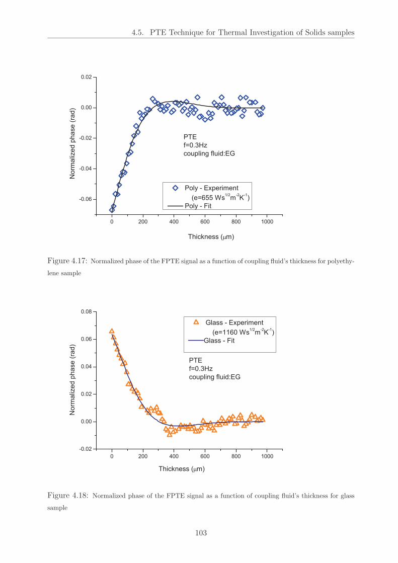
4.5. PTE Technique for Thermal Investigation of Solids samples
! " # $ %
& ' #
& ' "
& ' !
'
' !
!"#$%&''() *+
, -
./01234
#5678"%9(.86":;-<
!"#$%&'()*+,$-(*."$)/
(,58=(>(-?7&@"*&%A
)&/BCC(D'
EFG
*
>G
H
>E
+
(,58=(>(I"A
Figure 4.17: Normalized phase of the FPTE signal as a function of coupling fluid’s thickness for polyethy-
lene sample
! " # $ %
& ' !
'
' !
' "
' #
' $
!"
#$%&'()
*+,-./012#.,/34"5
!6/*708992: ;<
!"#$%&'()*+,$-(*."$)/
25.=992>2"?-8@/;80A
:8$BBC%2D9
BEF
;
>F
G
>B
<
5.=992>2H/A
Figure 4.18: Normalized phase of the FPTE signal as a function of coupling fluid’s thickness for glass
sample
103

4.5. PTE Technique for Thermal Investigation of Solids samples
! " # $% $ $! $" $#
&!%
& %
%
%
!%
"%
#%
$%%
$ %
$!%
$"%
$#%
!"#$$
%&'' ()*+,-
./01'2(3
%45"'#6*7#(*54 $*84#6-
!"#$%&'(#)*(+,
9"1:;14+3 %<7-
Figure 4.19: Experimental PTE phase signals as a function of frequency, in back configuration, for the
brass/TE assembly (blue squares) and for the empty sensor (red circles).
!" ! !# !$ !% &!" &! &!# &!$ &!% #!" #!
' !%
' !$
' !#
' !
' !"
'(!%
!"#$%&'(! )*+""),-./01
$2#%&345363
7*+8465)9:;34<51)=+3
;<
"
>
:
!"#$%&'()*+,$-(*."$)/
?(,*@1)*AB1
)C=#%(."%D,!$)
)E.,
Figure 4.20: Normalized phase as a function of sqrt(f) for the BPTE signal from brass sample.
104

4.5. PTE Technique for Thermal Investigation of Solids samples
single crystal. Their room temperature values of the thermal diffusivities are displayed in
table 4.5 together with the values measured using PPE and infrared thermography (IR-
thermography) techniques on the same samples. These measured values are also in good
agreement with the available literature data [143, 145].
!" !# !$ %! %!& #!"
'%!"
' !(
' !"
')!(
')!"
'"!(
!"#$%
&
'()*++ ,-"./0
12$33
'4++ ,-"./0
$56+"76+ $5589
'4++ ,-"./0
!"#$%&'()*+,$-(*."$)/
3:2,';0 '<=
4>?
0
Figure 4.21: Normalized phases of the PTE signals, in back configuration, as a function of sqrt(f) for
brass (violet circles), Al (red diamonds) and LiTaO3 (green squares).
Table 4.5: Thermal diffusivities of aluminium, brass and LiTaO3 measured using PTE, PPE and IR-
thermography techniques.
MaterialThermal Diffusivity (×10−6m2/s)
PTE PPE IR-Thermography
Aluminium (alloy) 27.20±0.57 36.94±0.20 30±1
Brass 19.34±0.64 17.93±0.21 20±1
LiTaO3 1.24±0.03 1.00±0.01 —
4.5.5.2 Summary of PTE Experimental Results on Solid Samples
The theory of the two detection configurations was developed and the results compared
with PPE technique in section 4.5.3. In principle, the general results obtained for the PTE
105

4.6. Summary
voltage in both front and back configurations are different from PPE ones, but when using
particular cases of experimental interest ((i) front configuration with opaque sensor, ther-
mally thin sensor and coupling fluid, and semi-infinite backing, or (ii) back configuration
with optically opaque sample and thermally thick sample and sensor) they are identical.
Consequently, the only differences and possible advantages of this new technique come
from the values of the sensors’ (pyro and TE) thermal and/or electrical parameters. For
example, in the case of the TE used in this work, both thermal effusivity and diffusivity
of the TE are about 3 times smaller than the similar parameters of a LiTaO3 pyroelectric
sensor. Consequently, in order to fulfil the conditions for particular detection cases (ther-
mally thin/thick regime for different layers of the detection cell), different ranges for the
scanning parameters are required. This can be an advantage or disadvantage, depending
on the type of investigated material. A huge difference between the TE and pyroelectric
sensors is their electrical resistivity. From experimental point of view, the low electrical
resistivity (few Ohms) of TE is correlated with low signal voltage (tens of µV), but also
with very low noise signal (tens of nV). The typical S/N ratio is larger than 102 -103, simi-
lar with that obtained with pyroelectric sensors. To go on with the comparison of the two
methods, the PTE needs higher levels of incident radiation (hundreds of mW), but the TE
generators are not limited in temperature by a critical one, as in the case of pyroelectric
sensors (Curie point).
Here, some applications on some solids, covering a large range for the typical values
of thermal parameters (Aluminium, Glass, Teflon, Polyethylene and even a largely used
pyroelectric material, LiTaO3), were described, in order to demonstrate the suitability of
the method. The results obtained for the values of the thermal parameters are in agreement
with literature data. In conclusion, a new photothermal technique, the photothermoelectric
method, was proposed for calorimetric investigations. The method is an alternative to the
PPE; it is very similar with the PPE technique, but it is based on a new class of materials
with different properties.
4.6 Summary
A novel technique, based on the photothermoelectric (PTE) effect has been introduced
for thermal characterization of TE generators. For that, the voltage generated in TE sen-
106

4.6. Summary
sors due to the temperature variations between the two sides were modelled in terms of
temperature fields and solved the heat diffusion equations. As obtained, equations for tem-
perature fields contains the thermal transport properties of TE material. Thereby, we can
thermally characterize the thermoelectrics without using a secondary sensing mechanism.
We have also proposed the very same technique as an alternative calorimetry tech-
nique for measuring dynamic thermal parameters of solid samples. In order to show the
various technical possibilities, we have used both back and front detection configurations,
coupled with laser chopping frequency as well as thickness scanning procedures. The front
PTE configuration, together with the thermal-wave resonator cavity (TWRC) method as
scanning procedure, has been used to measure the value of thermal effusivity. The back
PTE configuration, together with the chopping frequency of incident radiation as scan-
ning parameter, lead to the direct measurement of thermal diffusivity. The theory of the
two detection configurations was developed. In principle, the general results obtained for
the PTE voltage in both front and back configurations are different from PPE ones, but
when using particular cases of experimental interest ((i) front configuration with opaque
sensor, thermally thin sensor and coupling fluid, and semi-infinite backing, or (ii) back
configuration with optically opaque sample and thermally thick sample and sensor) they
are identical.
107

General Conclusions and Future
Outlook
This thesis work is intended to investigate on the thermal transport properties of material
composites using photothermal techniques. As a continuation of past research works in
our laboratory, this work is aimed to study thermal properties of two different classes of
technologically important materials. The first class deals with polymer dispersed liquid
crystals and the second class is about thermoelectric (TE) polymer nano composites.
Polymer dispersed liquid crystal (PDLC) samples are chosen because of their rich phys-
ical properties, so that we can consider them as a model system to interpret many physical
phenomena. One of its interesting nature is coming from the heterogeneity of the system
by the presence of spherical inclusions of liquid crystals whose thermophysical properties
can be controlled by external means without making any physical interruption to the sam-
ple system. The PDLC samples used in this studies are made of polystyrene (PS) and
4-Cyano-4’-pentylbiphenyl (5CB) liquid crystal. Samples having two different liquid crys-
tal (LC) concentrations (73 wt% and 85 wt%) were prepared using a procedure based on
solvent induced phase separation (SIPS).
We have chosen photothermal radiometry (PTR) technique to investigate the thermal
properties of samples because of the experimental simplicity and non-contact nature. The
latter property helps to conduct measurements on samples under external electric field
with greater freedom in sample cell erection than contact photothermal (PT) methods.
In order to perform the thermal investigations with high accuracy and resolution similar
to the one obtained using contact PT techniques like photopyroelectric (PPE), we have
developed novel methods with PTR, so called back-front-PTR (BF-PTR) and back-PTR
(B-PTR), to study liquid samples. In this novel approach, a small amount (about 5 µl) of
liquid sample is enclosed between two transparent windows (a quvette is used as bottom
108

General Conclusions and Future Outlook
window having known sample space thickness) in which the top window (made of CaF2
and facing PTR detector) has been chosen so that it is transparent to infrared radiation
specified by the detector. The sample cell is prepared to contain sample at the middle and
thin opaque coatings are made at faces of each top and bottom windows on the sample
touching surface to obtain laser heating exactly at the surface of the sample. In B-PTR,
the heating of the sample is from the bottom window side for both the sample and reference
scans. This method gives thermal diffusivity and effusivity of the sample. But the sample
has to be replaced by a reference liquid for realizing the reference scan. Apart from this, in
BF-PTR configuration, there is no sample replacement needed, while, frequency scans of
the laser intensity modulations are performed from bottom side is normalized by a second
frequency scan of the sample from top. Here, thermal diffusivity is the only parameter
which can be deduced.
Both PTR methods are validated and compared with results from existing techniques and
found they can be used for the thermal characterization of liquid samples with high accu-
racy and certainty. A possible disadvantage of these methods are coming from the higher
laser power (a few tens of milliwatts) to be used for sample heating than compared to the
PPE techniques. This may limit the temperature resolution in the case of high resolution
phase transition studies are being performed.
We have studied thermal transport properties of PDLC samples under amplitude vary-
ing (at fixed frequency) and frequency varying (at fixed amplitude) electric field (EF). The
measurements have been carried out using B-PTR configuration. Here, the EF varying
results are obtained using experiments with single chopping frequency of the laser source,
which is one of the advantages of this configuration if the sample properties are known at
zero electric field.
The amplitude (of the EF) varying experiments are confirming our already published
works and the frequency (of the EF) varying experiments clearly showing the Maxwell-
Wagner-Sillars (MWS) effect (polarization field effect) on thermal properties of PDLC
samples. Relations between thermal conductivity of PDLCs and existing MWS model are
established and the results are numerically fitted to find electrical properties (electrical
conductivities of PS and LC as well as the threshold electric field (E0) for LC droplet
alignment) of both PDLC samples (of 73% LC and 85% LC). Obtained results for E0 has
been used to calculate droplet elastic constants. Our results are showing that the amplitude
109

General Conclusions and Future Outlook
of the threshold electric field increases with reducing droplet size (or LC concentration) as
expected.
An interesting outcome of PDLC results from frequency (of EF) varying experiments
have shown, for the first time to the best of our knowledge, that the thermal transport
through PDLCs can be controlled via changing the frequency of the applied EF. In other
words, the thermal transport properties of PDLC films are also affected by depolarization
field effects as in the case of optical transmission properties. Moreover, the experimental
results give access to find various physical properties such as: elastic constants, threshold
electric field, Kapitza resistance, average molecular long axis orientation of LC droplets.
The second part of this thesis work is concerned about thermal investigation of ther-
moelectric (TE) polymer nano-composites. Studies on TE materials are particularly inter-
esting because of their growing importance in waste heat energy harvesting technology. As
part of this work, we have developed novel photothermal technique based on photother-
moelectric (PTE) effect to measure thermal properties of TE materials directly. The PTE
technique is established theoretically and validated experimentally by finding thermal prop-
erties of the same set of samples using classical photothermal radiometry technique. The
samples used are composites made of polyaniline (PANI), a widely used conducting poly-
mer, and carbon nanotubes (CNT). Four sample composites are prepared at 6.6 wt% of
four kinds of CNTs (un-oxidized or oxidized / single or multi walled nanotubes). Compar-
ing with other already reported studies on PANI-CNT materials, our samples are stay aside
due to its novel preparation method and oxidation levels of CNTs. A chemical synthesis
procedure in which the CNTs are wrapped around by PANI and form hybridized compos-
ites via an in situation polymerization procedure. Scanning electron microscope (SEM)
images of these as grown PANI-CNT composites are used to confirm their physical struc-
tures. Results from thermal properties of these samples showed that single walled CNT
composites are more thermally conductive than multi-walled CNT composites. Moreover,
composites with oxidized nanotubes have lower conductivity than their unoxidised counter
parts. The results have shown that the maximum enhancement in thermal conductivity
is only about 2.5 times higher than the pure PANI sample while the measured electrical
conductivity and seebeck coefficients are about 650 times and 6 times higher than pure
PANI, respectively. This observation is particularly interesting and highly recommended
because, the efficiency of TE materials are proportional to electrical conductivity and see-
110

General Conclusions and Future Outlook
beck coefficient while it is inversely proportional to sample’s thermal conductivity. The
experimental observations are analysed in the light of nanotube physical properties and
interfacial thermal resistance.
We have also described PTE technique for measuring thermal properties of solid sam-
ples while using TE materials as thermal sensors. The developed techniques are classified
under back-PTE (B-PTE), in which the sample is periodically heated directly, and front-
PTE (F-PTE), in which the sensor is heated directly. In B-PTE, a scan has been done by
varying laser chopping frequency and the thermal diffusivity is the outcome. On the other
hand, in F-PTE, a thickness scan of the coupling fluid in between the sample and sensor is
used to find sample’s thermal effusivity. Validation experiments have been conducted by
choosing solid samples in wide range of thermal properties.
This novel PTE technique has some notable advantages like, possibility of direct ther-
mal characterization of TE materials and its inherent simplicity. This technique can be
used to thermally characterize different TE materials regardless their nature (polymers,
glasses, metallic or semiconducting materials). At the same time, due to the lower electri-
cal resistivity of used TE materials, the noise levels were observed as low as 50 nV in the
experimental frequency domain. On the other hand, a higher laser power (about 750 mW
at 8 mm spot size) is used to conduct the experiments.
This thesis primarily focused on the investigation of thermal transport studies of PDLC
samples. Studies on these system’s thermophysical properties vs. temperature, LC concen-
tration, various kinds of LCs and polymer matrix will help to understand thermal transport
behaviour in different circumstances. In a thermal point of view, these studies not only help
to understand fundamental heat transport in heterogeneous systems but also contribute to
the developments of electrically controlled heat shutters.
In the field of thermoelectric material research, a broad and extensive research works
are being conducted by various research teams around the world to develop high efficient
heat conversion materials. Our works on the thermal behaviour of certain samples by a
chosen method must be investigated further by different nanotube concentrations, lengths
of nanotubes, different host polymer matrices etc. in order to optimize them for producing
highest efficiency. More than that, samples prepared by various methods (e.g., mechanical
mixing, in situation polymerization and so on) could give more insight on the thermal
transport through nano-composites and the role of Kapitza resistance with respect to
111

General Conclusions and Future Outlook
nanotube addition to the host matrix. Temperature dependent measurements are also
needed to predict their performances in different temperatures.
As part of the PTE technique, further studies are needed to develop or find sensors which
work at lower laser powers. This could be directly related to the Seebeck coefficients of
materials. At the same time materials with higher electrical resistance (typically more than
a few tens of ohms through sensor thickness) is preferable for the collection of generated
majority carriers from both surface of the sensor efficiently via thin coatings.
112

Appendix
Beer-Lambert law: If I be the intensity of the transmitted light through a layer of
material with thickness z for an incident intensity of radiation I0. According to Beer-
Lambert law:
I = I0e−βz, (z ≥ 0)
where, β is known as the attenuation coefficient (or optical absorption coefficient), given
by:
β = −1
zln
(
I
I0
)
In such condition for absorption, the optical intensity of the light wave, (I), is exponentially
reduced while travelling through the medium. Reciprocal of β is called penetration depth,
the depth at which the intensity reduced by a factor of 1/e of the original signal.
Extinction Coefficient: The optical absorption coefficient can also be expressed as,
β = 4πK/λ
where, λ is the wavelength of the incident radiation and K is the extinction coefficient.
Solving by separation of variable method: The temperature field (T (z, t)), function
of space and time, can be expressed as the product of two ordinary differential equations,
given by:
T (z, t) = F (z)G(τ) (A-1)
Substituting eq. (A-1) into eq. (2.12) and dividing by the product f g and excluding the
source term gives:
α1
F
d2F
dz2=
1
G
dG
dτ(A-2)
113

Appendix
Since both sides of the eq. (A-2) can vary quite independently of each other, the only
way that this can happen is if the two side are equal to a constant. So both sides of the
equation can be written as:
α1
F
d2F
dz2= Λ (A-3)
1
G
dG
dτ= Λ (A-4)
Substituting eq. (2.13) in eq. (A-4) for the time dependance gives:
1
G
dG
dτ= Λ =
1
eiωtiω eiωt = iω (A-5)
Substituting Λ from eq. (A-5) in the z dependent eq. (A-4) gives:
d2F
dz2= iω
F
α(A-6)
This can also be expressed as an exponential solution, say [eσz].
114

Bibliography
[1] Michael J Rightley, John A Emerson, C Channy Wong, Dale L Huber, and Blake Jak-
aboski. Advancement in Thermal Interface Materials for Future High-Performance
Electronic Applications : Part 1. Technical Report February, Sandia National Lab-
oratories, 2007. (document)
[2] A P C Ribeiro, S I C Vieira, J M Franca, C S Queiros, E Langa, M J V Lourenco,
S M S Murshed, and C A Nieto De Castro. Thermal Properties of Ionic Liquids and
Ionanofluids. 2009. (document)
[3] Nidhi Dubey and Mario Leclerc. Conducting polymers: Efficient thermoelectric
materials. Journal of Polymer Science Part B: Polymer Physics, 49(7):467–475,
April 2011. (document), 4.2.2.1
[4] Donald Hopkins, Ronald H Brown, and Mary L Good. PREDICTING THE IGNI-
TION TIME AND BURNING RATE OF THERMOPLASTICS IN. (September),
1995. (document)
[5] Yulong Ding, Hajar Alias, Dongsheng Wen, and Richard A Williams. Heat transfer
of aqueous suspensions of carbon nanotubes (CNT nanofluids). International Journal
of Heat and Mass Transfer, 49(1-2):240–250, January 2006. (document)
[6] M. J. Assael, I. N. Metaxa, K. Kakosimos, and D. Constantinou. Thermal Conduc-
tivity of Nanofluids-Experimental and Theoretical. International Journal of Ther-
mophysics, 27(4):999–1017, August 2006. (document)
[7] Anna Matvienko, Andreas Mandelis, and Stephen Abrams. Robust multiparameter
method of evaluating the optical and thermal properties of a layered tissue struc-
115

Bibliography
ture using photothermal radiometry. Applied optics, 48(17):3192–203, June 2009.
(document)
[8] Zheyu Shen, Ken Terao, Yasuyuki Maki, Toshiaki Dobashi, Guanghui Ma, and Takao
Yamamoto. Synthesis and phase behavior of aqueous poly(N-isopropylacrylamide-co-
acrylamide), poly(N-isopropylacrylamide-co-N,N-dimethylacrylamide) and poly(N-
isopropylacrylamide-co-2-hydroxyethyl methacrylate). Colloid and Polymer Science,
284(9):1001–1007, April 2006. (document)
[9] Santhosh Onkaraiah and Chuan Seng Tan. Mitigating heat dissipation and thermo-
mechanical stress challenges in 3-D IC using thermal through silicon via (TTSV).
2010 Proceedings 60th Electronic Components and Technology Conference (ECTC),
pages 411–416, 2010. (document)
[10] http://techon.nikkeibp.co.jp/NEA/archive/200401/283392/. Design view from
japan: Oki electric tackles heat dissipation. (document)
[11] Bo Feng, Zhixin Li, and Xing Zhang. Prediction of size effect on thermal conductivity
of nanoscale metallic films. Thin Solid Films, 517(8):2803–2807, February 2009.
(document)
[12] S Y Lu and J L Song. Effect of interfacial characteristics on effective conductivities of
composites containing randomly distributed aligned long fibers. Chemical engineering
science, 51(19), 1996. (document)
[13] Sergei Shenogin. Role of thermal boundary resistance on the heat flow in carbon-
nanotube composites. Journal of Applied Physics, 95(12):8136, 2004. (document)
[14] S.S.A. Seo, H.N. Lee, and T.W. Noh. Infrared spectroscopy of CaTiO3, SrTiO3,
BaTiO3, Ba0.5Sr0.5TiO3 thin films, and (BaTiO3)5/(SrTiO3)5 superlattice grown
on SrRuO3/SrTiO3(001) substrates. Thin Solid Films, 486(1-2):94–97, August 2005.
(document)
[15] Stefan Zollner, A. A. Demkov, R. Liu, P. L. Fejes, R. B. Gregory, Prasad Alluri,
J. A. Curless, Z. Yu, J. Ramdani, R. Droopad, T. E. Tiwald, J. N. Hilfiker, and J. A.
Woollam. Optical properties of bulk and thin-film SrTiO 3 on Si and Pt. Journal of
vacuum science and technology. B, 18(4):2242–2254, 2000. (document)
116

Bibliography
[16] L. Liang and Baowen Li. Size-dependent thermal conductivity of nanoscale semicon-
ducting systems. Physical Review B, 73(15):1–4, April 2006. (document)
[17] F L A Richardson, S D Peacor, C. Uher, and Franc0 Nori. YBa2Cu307-a films :
Calculation path of the thermal conductiwity and phonon mean free path. Journal
of Applied Physics, 72(10):4788–4791, 1992. (document)
[18] David G. Cahill, Wayne K. Ford, Kenneth E. Goodson, Gerald D. Mahan, Arun
Majumdar, Humphrey J. Maris, Roberto Merlin, and Simon R. Phillpot. Nanoscale
thermal transport. Journal of Applied Physics, 93(2):793, 2003. (document)
[19] Nicolas Houriez. Etude du Transport Thermique dans des Fluides Complexes par
Calorimetrie Photopyroelectric. PhD thesis, UDSMM, Universite littoral cote d’opale,
Dunkerque, France, 2008. (document)
[20] T. Bouchaour, F. Benmouna, F. Roussel, J.-M. Buisine, X. Coqueret, M. Benmouna,
and U. Maschke. Equilibrium phase diagram of poly(2-phenoxyethylacrylate) and
5CB. Polymer, 42(4):1663–1667, February 2001. (document), 3.23
[21] U. Maschke, A. Daoudi, F. Benmouna, F. Roussel, J.M. Buisine, X. Coqueret, and
M. Benmouna. Equilibrium phase properties of polymer/liquid crystal blends: The-
ory and experiments. Molecular Crystals and Liquid Crystals, 365:1361–1369, 2001.
(document)
[22] Roch Chan Yu King, Frederick Roussel, Jean-Francois Brun, and Carole Gors. Car-
bon nanotube-polyaniline nanohybrids: Influence of the carbon nanotube character-
istics on the morphological, spectroscopic, electrical and thermoelectric properties.
Synthetic Metals, 162(15-16):1348–1356, September 2012. (document), 4.1, 4.2.2.2,
4.4
[23] Abdelhak Hadj Sahraoui, Sylvain Delenclos, Stephane Longuemart, and Dorin
Dadarlat. Heat transport in polymer-dispersed liquid crystals under electric field.
Journal of Applied Physics, 110(3):033510, 2011. (document), 3.2.1.2, 3.2.2.2, 3.3.4.1
[24] Sarah Darby. Literature review for the Energy Demand Research Project. PhD thesis,
University of Oxford. (document)
117

Bibliography
[25] Kenji Morita. Automotive power source in 21st century. JSAE Review, 24(July
2002):3–7, 2003. (document)
[26] Bruno Gervet. Global Warming is mainly a result of Heat Emissions. PhD thesis,
Lulea University of Technology, Sweden, 2007. (document)
[27] C. White, R. Steeper, and A. Lutz. The hydrogen-fueled internal combustion engine:
a technical review. International Journal of Hydrogen Energy, 31(10):1292–1305,
August 2006. (document)
[28] Thamir K Ibrahim, M M Rahman, and Ahmed N Abdalla. Improvement of gas
turbine performance based on inlet air cooling systems : A technical review. Inter-
national Journal of Physical Sciences, 6(4):620–627, 2011. (document)
[29] David Michael Rowe. Review THERMOELECTRIC WASTE HEAT RECOVERY
AS A RENEWABLE ENERGY SOURCE. International Journal of Innovations in
Energy Systems and Power, 1(1):13–23, 2006. (document), 4.1
[30] Harumi Yokokawa. Materials for clean energy conversion. (document)
[31] Alaxander Graham Bell. Production of Sound by Radiant Energy. Manufacturer
and Builder (1869 - 1894), 0013(7):156–158, July 1881. 1.1, 1.1
[32] Qifang He, Reeta Vyas, and R. Gupta. Theory of photothermal spectroscopy in an
optically dense fluid. Applied Optics, 36(9):1841–1859, 20 march 1997. 1.1
[33] Y.-X. Nie and L. Bertrand. Separation of surface and volume absorption by pho-
tothermal deflection. Journel of Applied Physics, 65(2):438–447, 15 January 1989.
1.1
[34] O.W. Kading, H. Skurk, A.A. Maznev, and E. Matthias. Transient thermal gratings
at surfaces for thermal characterization of bulk materials and thin films. Applied
Physics A, 61:253–261, 1995. 1.1
[35] V. Gusev, C. Desmet, W. Lauriks, C. Glorieux, and J. Thoen. Theory of Scholte,
leaky Rayleigh, and lateral wave excitation via the laser-induced thermoelastic effect.
Journel of Acoustic Society of America, 100(3):1514, september 1996. 1.1
118

Bibliography
[36] Andreas Mandelis and Martin M. Zver. Theory of photopyroelectric spectroscopy of
solids. Journel of Applied Physics, 57(9):4421, May 1985. 1.1, 1.2.1, 2.2, 3.1.2.2
[37] N. Kawaguchi, Y. Nagasaka, and A. Nagashima. Fully automated apparatus to
measure the thermal conductivity of liquids by the transient hot-wire method. Review
of Scientific Instruments, 56(9):1788, 1985. 1.2
[38] H. Takahashi, Y. Hiki, and Y. Kogure. An improved transient hot-wire method for
studying thermal transport in condensed matter. Review of Scientific Instruments,
65(9):2901, 1994. 1.2
[39] R. G. Richard and I. R. Shankland. A transient hot-wire method for measuring the
thermal conductivity of gases and liquids. International Journal of Thermophysics,
10(3):673–686, May 1989. 1.2
[40] David G. Cahill and R. O. Pohl. Thermal conductivity of amorphous solids above
the plateau. Physical Review B, 35(8):4067–4073, 1987. 1.2
[41] M. Chirtoc Mihailescu and G. Theory of the photopyroelectric method for inves-
tigation of optical and thermal materials properties. Physical Review B, 40, No:
14(November):9606–9617, 1989. 1.2.1
[42] Stephane Longuemart. Study on Liquid Crystal and ferro fluids using Photopyroelec-
tric Technique. theses, universite littoral cote d’opale, 2002. 1.2.1, 4.2.2.3
[43] S. Delenclos, D. Dadarlat, N. Houriez, S. Longuemart, C. Kolinsky, and A. Hadj
Sahraoui. On the accurate determination of thermal diffusivity of liquids by using
the photopyroelectric thickness scanning method. Review of Scientific Instruments,
78(2):024902, 2007. 1.2.1
[44] Dorin Dadarlat, Mircea Nicolae Pop, Mihaela Streza, Stephane Longuemart, Michael
Depriester, Abdelhak Hadj Sahraoui, and Viorica Simon. Combined FPPE-PTR
Calorimetry Involving TWRC Technique II. Experimental : Application to Thermal
Effusivity Measurements of Solids. International Journal of Thermophysics, pages
2092–2101, 2011. 1.2.1, 2.2.1, 3.2.4
119

Bibliography
[45] Preethy Chirukandath Menon, Ravindran Nair Rajesh, and Christ Glorieux. High
accuracy, self-calibrating photopyroelectric device for the absolute determination of
thermal conductivity and thermal effusivity of liquids. The Review of scientific in-
struments, 80(5):054904, May 2009. 1.2.1, 3.3, 3.2.2.1
[46] J Caerels, C Glorieux, and J Thoen. Photopyroelectric thermal wave setup for the
absolute measurement of the thermal conductivity of low density gases. Review of
Scientific Instruments, 71(9), 2000. 1.2.1
[47] U. Zammit, M. Marinelli, F. Mercuri, S. Paoloni, and F. Scudieri. Invited Review
Article: Photopyroelectric calorimeter for the simultaneous thermal, optical, and
structural characterization of samples over phase transitions. The Review of scientific
instruments, 82(12):121101, December 2011. 1.2.1, 1.3.4
[48] M M Farrow, R K Burnham, M Auzanneau, S L Olsen, N Purdie, and E M Eyring.
Piezoelectric detection of photoacoustic signals. Applied optics, 17(7):1093–8, April
1978. 1.2.2
[49] A Hordvik and L Skolnik. Photoacoustic measurements of surface and bulk absorp-
tion in HF/DF laser window materials. Applied optics, 16(11):2919–24, November
1977. 1.2.2
[50] Per Helander and Ingemar Lundstrom. Separation of bulk and surface light adsorp-
tion with an open photoacoustic cell. Journal of Applied Physics, 54(9):5069, 1983.
1.2.2
[51] Maju Kuriakose, Michael Depriester, Roch Chan Yu King, Frederick Roussel, and
Abdelhak Hadj Sahraoui. Photothermoelectric effect as a means for thermal charac-
terization of nanocomposites based on intrinsically conducting polymers and carbon
nanotubes. Journal of Applied Physics, 113(4):044502, 2013. 1.2.3
[52] L. B. Kreuzer. Ultralow Gas Concentration Infrared Absorption Spectroscopy. Jour-
nal of Applied Physics, 42(7):2934, 1971. 1.3.1
[53] A. Rosencwaig. Photoacoustic scpectroscopy of solids. Optics Communications,
7(4):305–308, April 1973. 1.3.1
120

Bibliography
[54] H Vargas and L. C. M. Miranda. Photoacoustic and related photothermal techniques
and related photothermal. Physics Reports, 161(2):43–101, 1988. 1.3.1, 1.3.4
[55] W B Jackson, N M Amer, a C Boccara, and D Fournier. Photothermal deflection
spectroscopy and detection. Applied optics, 20(8):1333–44, April 1981. 1.3.2
[56] A. C. Boccara, D. Fournier, and J. Badoz. Thermo-optical spectroscopy: Detection
by the “mirage effect”. Applied Physics Letters, 36(2):130, 1980. 1.3.2
[57] Yongwu Yang and Keith A Nelson. Impulsive stimulated light scattering from
glass-forming liquids. I. Generalized hydrodynamics approach. Journal of Chemi-
cal Physics, 103(June):7722–7731, 1995. 1.3.3
[58] A.A. Maznev, K.A. Nelson, and J. A. Rogers. Optical heterodyne detection of laser-
induced gratings. Optics letters, 23(16):1319–21, August 1998. 1.3.3
[59] Rebecca M. Slayton, Keith a. Nelson, and a. a. Maznev. Transient grating mea-
surements of film thickness in multilayer metal films. Journal of Applied Physics,
90(9):4392, 2001. 1.3.3
[60] Dora M Paolucci and Keith A Nelson. Impulsive stimulated thermal scattering study
of structural relaxation in supercooled glycerol. Journal of Chemical Physics, 112(15),
2000. 1.3.3
[61] John A Rogers and Keith A Nelson. Study of Lamb acoustic waveguide modes in un-
supported polyimide f Urns using real-time impulsive stimulated thermal scattering.
Journal of Applied Physics, 75(3):1534–1556, 1994. 1.3.3
[62] A Mandelis, A Othonos, and C Christofides. Non-contacting measurements of photo-
carrier lifetimes in bulk- and polycrystalline thin-film Si photoconductive devices by
photothermal radiometry. Journal of Applied Physics, 80(9):5332–5341, 1996. 1.3.4
[63] H. Vargas and L. C. M. Miranda. Photothermal techniques applied to thermophysi-
cal properties measurements (plenary). Review of Scientific Instruments, 74(1):794,
2003. 1.3.4, 3.1.3
[64] G Busse. Optoacoustic and photothermal material inspection techniques. Applied
optics, 21(1):107–10, January 1982. 1.3.4
121

Bibliography
[65] D. P. Almond and P. M. Patel. Photothermal Science and Techniques. chapman &
Hall, 1996. 1.3.4, 2.1, 3.1.3
[66] Agustın Salazar. Energy propagation of thermal waves. European Journal of Physics,
27(6):1349–1355, November 2006. 2.1
[67] Allan Rosencwaig and Allen Gersho. Theory of the photoacoustic effect with solids.
Journal of Applied Physics, 47(1):64–69, January 1976. 2.1, 2.2
[68] R. Santos and L. C. M. Miranda. Theory of the photothermal radiometry with solids.
Journal of Applied Physics, 52(6):4194, 1981. 2.2, 3.1
[69] A. L. Edwards. A Compilation of Thermal Property Data for Computer Heat-
Conduction Calculations. UCRL-50589, University of California Lawrence Radiation
Laboratory, 24 February 1969. 2.2.1
[70] D. Dadarlat. Photopyroelectric calorimetry of liquids; recent development and ap-
plications. Laser Physics, 19(6):1330–1339, June 2009. 2.2.1, 3.2.4, 4.5.5
[71] Per-Erik Nordal and Svein Otto Kanstad. Photothermal Radiometry. Physica
Scripta, 20:659–662, 1979. 3.1
[72] S. J. Sheard and M. G. Somekh. Measurement of opaque coating thickness using
photothermal radiometry. Applied Physics Letters, 53(26):2715, 1988. 3.1
[73] H. P. R. Frederikse and X. T. Ying. Heat conductivity of oxide coatings by photother-
mal radiometry between 293 and 1173 K. Applied optics, 27(22):4672–5, November
1988. 3.1
[74] Jean Lazare and Nzodoum Fotsing. Investigation of Thermal Transport in Layered
Sytems and Micro-structured Semiconductor Devices by Photothermal Techniques
and Finite Element Simulations. PhD thesis, 2004. 3.1
[75] Eric P. Visser, Erwin H. Versteegen, and Willem J. P. van Enckevort. Measurement
of thermal diffusion in thin films using a modulated laser technique: Application
to chemical-vapor-deposited diamond films. Journal of Applied Physics, 71(7):3238,
1992. 3.1
122

Bibliography
[76] A. Kusiak, Ch. Pradere, and J. L. Battaglia. Measuring the thermal conductivity
of liquids using photo-thermal radiometry. Measurement Science and Technology,
21(1):015403, January 2010. 3.1
[77] K Sreekumar and V K Vaidyan. Measurement of thermal effusivity of liquids using
a photothermal imager. Measurement Science and Technology, 17(4):666–669, April
2006. 3.1
[78] Maju Kuriakose, Michael Depriester, Dorin Dadarlat, and Abdelhak Hadj Sahraoui.
Improved methods for measuring thermal parameters of liquid samples using pho-
tothermal infrared radiometry. Measurement Science and Technology, 24(2):025603,
February 2013. 3.1.2
[79] J. A. Balderas-Lopez and A. Mandelis. Self-normalized photothermal technique for
accurate thermal diffusivity measurements in thin metal layers. Review of Scientific
Instruments, 74(12):5219, 2003. 3.1.2.1, 4.5
[80] M. Chirtoc and G. Mihailescu. Theory of the photopyroelectric method for investi-
gation of optical and thermal materials properties. Physical Review B, 40(14):9606–
9617, November 1989. 3.1.2.2
[81] D. R. Lide. CRC Handbook of Chemistry and Physics 78th edition. CRC Press, Boca
Raton Newyork. 3.1, 3.2, 3.3, 3.4, 3.3.2
[82] M. Depriester, P. Hus, S. Delenclos, and A. Hadj Sahraoui. New methodology for
thermal parameter measurements in solids using photothermal radiometry. Review
of Scientific Instruments, 76(7):074902, 2005. 3.1.2.3, 4.3
[83] J A Balderas-lopez, Andreas Mandelis, and J A Garcıa. Measurements of the Thermal
Diffusivity of Liquids with a Thermal - Wave Resonator Cavity. Analytical Sciences,
17:519–522, 2001. 3.3
[84] Mitchell L Schlossman and Justin P Mccarthy. Lanolin and Its Derivatives. Journel
of the american oil chemists’ society, 447:447–450, 1977. 3.2.1.1
[85] M. Marinelli, F. Mercuri, U. Zammit, and F. Scudieri. Thermal conductivity and
thermal diffusivity of the cyanobiphenyl (nCB) homologous series. Physical Review
E, 58(5):5860–5866, 1998. 3.2.1.2, 3.2.2.3, 3.3.2, 3.5
123

Bibliography
[86] David D. Jackson. Most Squares Inversion. Journal of Geophysical Research,
81(5):1027–1030, 1976. 3.2.2.1
[87] Qingsheng Zeng, Sheng Wang, Leijing Yang, Zhenxing Wang, Tian Pei, Zhiyong
Zhang, Lian-Mao Peng, Weiwei Zhou, Jie Liu, Weiya Zhou, and Sishen Xie. Carbon
nanotube arrays based high-performance infrared photodetector [Invited]. Optical
Materials Express, 2(6):839, May 2012. 3.2.4
[88] J.L.Fergason. Polymer encapsulated nematic liquid crystals for display and light
control applications. SID Int. Symp. Dig. Tech. Pap., 16(4,435,047):68, 1985. 3.3
[89] J. W. Doane, N. a. Vaz, B.-G. Wu, and S. Zumer. Field controlled light scattering
from nematic microdroplets. Applied Physics Letters, 48(4):269, 1986. 3.3
[90] F. Basile, F. Bloisi, L. Vicari, and F. Simoni. Optical phase shift of polymer-dispersed
liquid crystals. Physical Review E, 48(1):432, 1993. 3.3
[91] Yi-Hsin Lin, Hongwen Ren, and Shin-Tson Wu. High contrast polymer-dispersed
liquid crystal in a 900 twisted cell. Applied Physics Letters, 84(20):4083, 2004. 3.3
[92] V. K. S. Hsiao and W.-T. Chang. Optically switchable, polarization-independent
holographic polymer dispersed liquid crystal (H-PDLC) gratings. Applied Physics B,
100(3):539–546, March 2010. 3.3
[93] V. A. Loiko and A. V. Konkolovich. Focusing of light by polymer-dispersed liquid-
crystal films with nanosized droplets. Journal of Experimental and Theoretical
Physics, 103(6):935–943, December 2006. 3.3
[94] R. W. Sillars. The properties of a dielectric containing semi- conducting particles
of various shapes. Wireless Section, Institution of Electrical Engineers, 80:378–394,
1937. 3.3.1
[95] Karl Willy Wagner. Erklarung der dielektrischen Nachwirkungsvorgange auf Grund
Maxwellscher Vorstellungen. Archiv fur Elektrotechnik, 2(9):371–387, September
1914. 3.3.1
[96] Ragab M. Soliman. Early Stages of Polymer Crystalization Studied by Dielectric
Spectroscopy. PhD thesis, Universitat Rostock, 2004. 3.3.1
124

Bibliography
[97] Mourad Boussoualem, Roch Chan Yu King, Jean-Francois Brun, Benoıt Duponchel,
Mimoun Ismaili, and Frederick Roussel. Electro-optic and dielectric properties of op-
tical switching devices based on liquid crystal dispersions and driven by conducting
polymer [poly(3,4-ethylene dioxythiophene):polystyrene sulfonate (PEDOT:PSS)]-
coated electrodes. Journal of Applied Physics, 108(11):113526, 2010. 3.3.1
[98] Jinwoo Han. Memory and Depolarization Effects of Polymer-Dispersed Liquid Crys-
tal Films Based on E7 / NOA61. Journal of the Korean Physical Society, 43(1):45–50,
2003. 3.3.1
[99] Mourad Boussoualem, Frederick Roussel, and Mimoun Ismaili. Thermophysical, di-
electric, and electro-optic properties of nematic liquid crystal droplets confined to a
thermoplastic polymer matrix. Physical Review E, 69(031702):1–10, 2004. 3.3.1
[100] Mourad Boussoualem, Mimoun Ismaili, Jean-Francois Lamonier, Jean-Marc Buisine,
and Frederick Roussel. Polarization field effects at liquid-crystal-droplet-polymer
interfaces. Physical Review E, 73(4):1–7, April 2006. 3.3.1
[101] Kelly J. R. and Seekola D. L. Dielectric losses in a polymer-dispersed liquid crystal
film. volume 1257 of Liquid Crystal Displays and Applications. Proc. SPIE, 1990.
3.3.1
[102] P. S. Drzaic. Liquid Crystal Dispersion. World Scientific, Singapore, 1995. 3.3.1,
3.3.5.1, 3.3.5.3, 3.3.5.3
[103] F Roussel, Jm Buisine, U Maschke, X Coqueret, and F Benmouna. Phase diagrams
and morphology of polymer dispersed liquid crystals based on nematic-liquid-crystal-
monofunctional-acrylate mixtures. Physical review. E, Statistical physics, plasmas,
fluids, and related interdisciplinary topics, 62(2 Pt A):2310–6, August 2000. 3.3.1
[104] Farida Benmouna, Abdelylah Daoudi, Frederick Roussel, Jean-Marc Buisine, Xavier
Coqueret, and Ulrich Maschke. Equilibrium phase diagram of polystyrene and 8cb.
Journal of Polymer Science Part B: Polymer Physics, 37(15):1841–1848, 1999. 3.3.1
[105] G. W. Smith. Study of formation, phase behavior, and microdroplet size of a
polyurethane-based polymer-dispersed liquid crystal. Molecular Crystals and Liq-
uid Crystals Incorporating Nonlinear Optics, 180(2):201–222, 1990. 3.3.1
125

Bibliography
[106] G. Perrier and A. Bergeret. Maxwell-wagner-sillars relaxations in polystyrene-glass-
bead composites. Journel of Applied Physics, 77:2651, 1995. 3.3.2
[107] Bo Gestblom and Stanislaw Wrobel. A thin cell dielectric spectroscopy method for
liquid crystals. Liquid Crystals, 18(1):31–35, 1995. 3.3.2
[108] V. Allouchery. Theses. PhD thesis, Universite du littoral cote d’Opale, Dunkerque,
France, 2000. 3.3.2
[109] Abderrahim Boudenne and Smain Khaldi. Temperature and Liquid Crystal Concen-
tration Effect on Thermal Conductivity of Poly ( styrene ) Dispersed 5CB Liquid
Crystal. Journal of Applied Polymer Science, 89:481–486, 2003. 3.3.2
[110] Ce-Wen Nan, R. Birringer, David R. Clarke, and H. Gleiter. Effective thermal con-
ductivity of particulate composites with interfacial thermal resistance. Journal of
Applied Physics, 81(10):6692, 1997. 3.3.4.1
[111] J. W. Doane, A. Golemme, J. L. West, J. B. Whitehead Jr., and B. G. Wu. Polymer
Dispersed Liquid Crystals for Display Application. Molecular Crystals and Liquid
Crystals Incorporating Nonlinear Optics, 165(1):511, 1988. 3.3.5.3
[112] Terry Hendricks and William T. Choate. Engineering Scoping Study of Thermo-
electric Generator Systems for Industrial Waste Heat Recovery. Technical Report
November, 2006. 4.1
[113] G Jeffrey Snyder and Eric S Toberer. Complex thermoelectric materials. Nature
materials, 7(2):105–14, February 2008. 4.1
[114] Deyu Li, Scott T. Huxtable, Alexis R. Abramson, and Arun Majumdar. Thermal
Transport in Nanostructured Solid-State Cooling Devices. Journal of Heat Transfer,
127(1):108, 2005. 4.1
[115] Weishu Liu, Xiao Yan, Gang Chen, and Zhifeng Ren. Recent advances in thermo-
electric nanocomposites. Nano Energy, 1(1):42–56, January 2012. 4.1
[116] G Chen, T Zeng, T Borca-Tasciuc, and D Song. Phonon engineering in nanos-
tructures for solid-state energy conversion. Materials Science and Engineering: A,
292(2):155–161, November 2000. 4.1
126

Bibliography
[117] Hideki Shirakawa, Edwin J. Louis, Alan G. MacDiarmid, Chwan K. Chiang, and
Alan J. Heeger. Synthesis of electrically conducting organic polymers: halogen
derivatives of polyacetylene, (CH) x. Journal of the Chemical Society, Chemical
Communications, (16):578, 1977. 4.1
[118] A. J. Minnich, M. S. Dresselhaus, Z. F. Ren, and G. Chen. Bulk nanostructured ther-
moelectric materials: current research and future prospects. Energy & Environmental
Science, 2(5):466, 2009. 4.1
[119] A. Mandelis. Diffusion-Wave Fields, Mathematical Methods and Green Functions.
Springer Verlag New York, 2001. 4.2
[120] A. Hadj Sahraoui, S. Longuemart, D. Dadarlat, S. Delenclos, C. Kolinsky, and J. M.
Buisine. The application of the photopyroelectric method for measuring the thermal
parameters of pyroelectric materials. Review of Scientific Instruments, 73(7):2766,
2002. 4.2
[121] D D Ateh, H a Navsaria, and P Vadgama. Polypyrrole-based conducting polymers
and interactions with biological tissues. Journal of the Royal Society, Interface / the
Royal Society, 3(11):741–52, December 2006. 4.2.2.1
[122] John D W Madden, Bryan Schmid, Martin Hechinger, Serge R Lafontaine, G A
Peter, Franz S Hover, Richard Kimball, and Ian W Hunter. Application of Polypyr-
role Actuators : Feasibility of Variable Camber Foils. IEEE Journal of Oceanic
Engineering, 2003. 4.2.2.1
[123] Eric Hu, Akif Kaynak, and Yuncang Li. Development of a cooling fabric from con-
ducting polymer coated fibres: Proof of concept. Synthetic Metals, 150(2):139–143,
April 2005. 4.2.2.1
[124] Uffana Riaz, S.M. Ashraf, and Sharif Ahmad. High performance corrosion protective
DGEBA/polypyrrole composite coatings. Progress in Organic Coatings, 59(2):138–
145, May 2007. 4.2.2.1
[125] Mihaela Baibarac and Pedro Gomez-Romero. Nanocomposites Based on Conduct-
ing Polymers and Carbon Nanotubes from Fancy Materials to Functional Applica-
127

Bibliography
tions. Journal of Nanoscience and Nanotechnology, 6(11):3325–3328, November 2006.
4.2.2.1
[126] Alan G Macdiarmid. ”Synthetic Metals” : A Novel Role for Organic Polymers (
Nobel Lecture ). Angew. Chem. Int. Ed, 40:2581–2590, 2001. 4.2.2.1
[127] Y. Xuan, X. Liu, S. Desbief, P. Leclere, M. Fahlman, R. Lazzaroni, M. Berggren,
J. Cornil, D. Emin, and X. Crispin. Thermoelectric properties of conducting poly-
mers: The case of poly(3-hexylthiophene). Physical Review B, 82(11):1–9, September
2010. 4.2.2.1
[128] Dasaroyong Kim, Yeonseok Kim, Kyungwho Choi, Jaime C Grunlan, and Choongho
Yu. Improved thermoelectric behavior of nanotube-filled polymer composites with
poly(3,4-ethylenedioxythiophene) poly(styrenesulfonate). ACS nano, 4(1):513–23,
January 2010. 4.2.2.1
[129] Kanishka Biswas, Jiaqing He, Ivan D Blum, Chun-I Wu, Timothy P Hogan, David N
Seidman, Vinayak P Dravid, and Mercouri G Kanatzidis. High-performance bulk
thermoelectrics with all-scale hierarchical architectures. Nature, 489(7416):414–8,
September 2012. 4.2.2.1
[130] M Chirtoc, E H Bentefour, C Glorieux, and J Thoen. Development of the front-
detection photopyroelectric ( FPPE ) configuration for thermophysical study of glass-
forming liquids. Thermochimica Acta, 377:105–112, 2001. 4.2.2.3
[131] H. K. Park, C. P. Grigoropoulos, and A. C. Tam. Optical Measurements of Thermal
Diffusivity of a Material. International Journal of Thermophysics, 16(4):973–995,
1995. 4.3
[132] Jyotsna Ravi, Yuekai Lu, Stephane Longuemart, Stefano Paoloni, Helge Pfeiffer, Jan
Thoen, and Christ Glorieux. Optothermal depth profiling by neural network infrared
radiometry signal recognition. Journal of Applied Physics, 97(1):014701, 2005. 4.3
[133] M. Streza, D. Dadarlat, M. N. Pop, C. Prejmerean, D. Prodan, M. Depriester,
S. Longuemart, and A. Hadj Sahraoui. Photothermal radiometry (PTR) investi-
gation of dynamic thermal parameters of dental composites. Optoelectronics and
Advanced Materials-Rapid Communications, 4(11):1830–1834, 2010. 4.3, 4.3
128

Bibliography
[134] Michael Depriester. Study on carbon nanotube based composites using photothermal
radiometry. PhD thesis, Universite littoral cote d’Opale, 2007. 4.3
[135] Ce-Wen Nan, Gang Liu, Yuanhua Lin, and Ming Li. Interface effect on thermal
conductivity of carbon nanotube composites. Applied Physics Letters, 85(16):3549,
2004. 4.4
[136] Jun Shen and Andreas Mandelis. Thermal-wave resonator cavity. Review of Scientific
Instruments, 66(10):4999–5005, 1995. 4.5
[137] J. A. Balderas-Lopez, A. Mandelis, and J. A. Garcia. Thermal-wave resonator cavity
design and measurements of the thermal diffusivity of liquids. Review of Scientific
Instruments, 71(7):2933, 2000. 4.5
[138] M. Marinelli, F. Mercuri, U. Zammit, R. Pizzoferrato, F. Scudieri, and D. Dadarlat.
Photopyroelectric study of specific heat, thermal conductivity, and thermal diffusivity
of Cr2O3 at the Neel transition. Physical Review B, 49(14):9523–9532, 1994. 4.5
[139] D. Dadarlat, M. Streza, M. N. Pop, V. Tosa, S. Delenclos, S. Longuemart, and a. Hadj
Sahraoui. Photopyroelectric calorimetry of solids. Journal of Thermal Analysis and
Calorimetry, 101(1):397–402, November 2009. 4.5.3
[140] Dorin Dadarlat and Camelia Neamtu. High Performance Photopyroelectric Calorime-
try of Liquids. Acta Chim. Slov., 56:225–236, 2009. 4.5.4
[141] Chirtoc M., Antoniov J. S., and Egee M. The Effective Thermal Thickness: A New
Concept for Photothermal Investigation of Layered Systems. In Proc 10-th Int. Conf.
on Photoacoustic and Photothermal Phenomena (Rome, 84-86), 1998. 4.5.5
[142] A Mandelis. Principles and perspectives of photothermal and photoacoustic phenom-
ena. New York: Elsevier, 1992. 4.5.5.1
[143] D. Dadarlat. Contact and non-contact photothermal calorimetry for investigation
of condensed matter. Journal of Thermal Analysis and Calorimetry, 110(1):27–35,
January 2012. 4.5.5.1, 4.5.5.1
[144] Touloukian YS. Thermophysical Properties of High Temperatures Solid Materials.
New York: MacMillan, 1967. 4.5.5.1
129

Bibliography
[145] Masaru Nakamura, Shunji Takekawa, and Kenji Kitamura. Anisotropy of thermal
conductivities in non- and Mg-doped near-stoichiometric LiTaO3 crystals. Optical
Materials, 32(11):1410–1412, September 2010. 4.5.5.1
130