Oil Sands Process-Affected Water Toxicity Attribution

and Evaluating Ageing as a Remediation Strategy

by

Ian George Michael Gault

A thesis submitted in partial fulfillment of the requirements for the degree of

Master of Science

in

Analytical & Environmental Toxicology

Department of Laboratory Medicine and Pathology

University of Alberta

© Ian George Michael Gault, 2019

ii

Abstract

Oil sands process-affected water (OSPW) is a byproduct of bitumen extraction in the surface-

mining oil sands industry of Northern Alberta. OSPW contains a complex and environmentally

persistent dissolved organic mixture that can be toxic to aquatic organisms. One long-term

remediation strategy involves ageing of OSPW in end-pit lakes such that in situ natural processes

will eventually allow detoxification and safe environmental re-integration of this water. Over 30

end-pit lakes are planned, but only one has been established so far, Base Mine Lake (BML),

which was commissioned in 2012 at Syncrude Canada Ltd. Predicting the effectiveness of this

strategy relies on an understanding of what chemicals cause toxicity in fresh OSPW, and how the

chemical mixture might change over time. This investigation used chemical fractionation and

ultrahigh resolution mass spectrometry combined with cytotoxicity and endocrine disruption

assays to further study the toxicity of candidate chemical classes in fresh and aged OSPW

samples. Real-time cell analysis with human liver carcinoma cells (HepG2) was used with

OSPW samples for the first time, while the yeast estrogenic/androgenic screens were used as a

standardized and comparable assay to previous studies. A chemical fraction isolated from BML

2015 containing naphthenic acids (NAs) was largely responsible for the cytotoxicity observed

towards HepG2 cells, with a point of departure (IC10) at 17 mg/L, similar to the estimated field

concentration of NAs in BML 2015 (12.9 mg/L). A corresponding non-acid fraction, speculated

to contain steroid-like chemicals, was not cytotoxic up to 12.5× above field concentrations in

BML 2015. The total organic extract of BML 2017 was cytotoxic to HepG2 cells, generating an

IC50 of 8× above field concentrations, with the point of departure marginally above 1×. Based on

a series of BML water samples collected over a 4-year span, the cytotoxicity of BML extracts

(i.e. toxicity per volume) decreased with ageing, while the toxic potency of the extracts (toxicity

iii

per mass of extract) was not significantly different between years. This toxicological result was

supported by mass spectral evidence whereby total m/z intensity of BML organics decreased in

samples over time, but the relative proportion of chemical classes remained unchanged. Older

OSPW aged 23 years in an experimental pond had a unique biphasic toxicity profile (time-

dependent), with a toxic potency greater than BML at 24 h post exposure, but not at 60 h. This

sample also had a unique distribution of chemical classes compared to BML. Estrogen and

androgen receptor antagonists, but not agonists, were identified in all BML 2015 fractions.

Notably, the NA and non-acidic fractions showed endocrine activity below environmentally

relevant concentrations and were more potent (toxicity per mass of extract) than positive control

antagonistic hormones. Overall, with BML and experimental pond samples ranging up to 23

years of ageing in the field, there was little difference in the potency of estrogen and androgen

receptor antagonism between the organic extracts, and always with EC50’s below environmental

concentrations and similar to positive control antagonistic hormones. While organic acids,

including naphthenic acids, decreased to a large extent in the aged samples, chemical classes

detected in positive mode (i.e. polar organics) were less depleted and became relatively enriched

in the total organic extract, suggesting that non-acid polar organics contribute to environmentally

persistent estrogen and androgen receptor antagonism. Overall, decreases in cytotoxicity in BML

over time, although promising for the end-pit lake strategy, are likely only due to a dilution

effect. Also, this is the first report of an older experimental pond sample having a biphasic

cytotoxicity profile, which, along with its chemical profile, remains to be understood. This

highlights the importance of chemical composition, not only concentration, in determining risk,

and warrants further research into chemical-specific regulatory limits needed to ensure

environmental protection.

iv

Preface

This thesis is original work by Ian Gault. No part of this thesis has been previously published.

v

Acknowledgements

I would like to thank my supervisor, Dr. Jonathan Martin, for his support and guidance

during my master’s program. Many of the professional goals I looked to achieve in my masters

were enabled by his intellectual freedom and style in teaching, research, and writing. I would

also like to thank the contributions of my supervisory committee, Dr. Xing-fang Li and Dr.

Monika Keelan, for their mentorship and research expertise. Also, thank you to NSERC for the

CRD grant, and to the University of Alberta for scholarship opportunities.

I would like to thank Dr. Birget Moe for her unwavering support, training, and

troubleshooting with cell cultures and bioassays – you helped lay the foundation for my work.

Furthermore, thank you Dr. Chenxing Sun for your technical training and work with OSPW and

mass spectrometry. Lastly, thank you Evelyn Aseidu, my fellow graduate student in OSPW

research in the Martin group, who helped me navigate the research area with her insights and

training, and became a close friend. I would also like to thank the entire Martin group: Yifeng,

Anthony, Jiaying, and Hannah, for their stimulating, high-level discussions, their friendship, and

for broadening my own research knowledge in lab meetings and other mediums. Furthermore,

thanks to the entire AET division in Dr. Chris Le’s, Dr. Xing-fang Li’s, and Dr. Hongquan

Zhang’s group for providing such a supportive lab environment. I sincerely thank Ms. Katerina

Carastathis, Ms. Diane Sergy, and Ms. Cheryl Titus who helped me navigate the administrative

aspects of graduate school and continuously brought me peace of mind.

I sincerely thank my parents, Siobhan and Michael, and my siblings, Anna, Monica,

Caroline, and David, for their endless support, love, and guidance. My masters coincided with

considerable personal change and development, so I thank a few of my friends – Tristan,

Thomas, Lucy, Jade, Jacob, and Cam – for keeping my life balanced, exciting, and supported.

vi

Table of Contents

1. Introduction ............................................................................................................................. 1

1.1. Oil sands in Alberta ................................................................................................................... 1

1.1.1. Location, features, and demand for energy ......................................................................... 1

1.1.2. Open pit oil sands mining ................................................................................................... 2

1.1.3. Environmental challenges with open pit mining................................................................. 4

1.1.3.1. Water management ....................................................................................................................... 4

1.1.3.2. Land disturbances ......................................................................................................................... 8

1.1.3.3. Contamination of the environment ............................................................................................... 8

1.1.4. Environmental regulation of open pit mining ................................................................... 11

1.2. Oil sands process-affected water (OSPW) ............................................................................. 12

1.2.1. Parameters affecting detection of species ......................................................................... 15

1.2.1.1. Resolution .................................................................................................................................. 15

1.2.1.2. Ionization source ........................................................................................................................ 15

1.2.1.3. Extraction method ...................................................................................................................... 16

1.2.2. Persistence of OSPW organics.......................................................................................... 18

1.2.2.1. Natural biodegradation ............................................................................................................... 19

1.2.2.2. Other treatment strategies ........................................................................................................... 20

1.2.3. Environmental fate ............................................................................................................ 21

1.2.4. Exposure ........................................................................................................................... 22

1.2.4.1. Toxicokinetics ............................................................................................................................ 22

1.2.4.2. Biomonitoring of the surrounding area ...................................................................................... 23

1.3. OSPW toxicity .......................................................................................................................... 24

1.3.1. Toxicity attribution ........................................................................................................... 24

1.3.2. In vivo laboratory studies .................................................................................................. 28

1.3.3. Cytotoxicity ...................................................................................................................... 30

vii

1.3.3.1. Real-Time Cell Analysis (RTCA) .............................................................................................. 32

1.3.4. Oxidative stress ................................................................................................................. 33

1.3.5. Endocrine disruption ......................................................................................................... 34

1.3.6. Base Mine Lake (BML) toxicity ....................................................................................... 38

1.4. Rationale for thesis research .................................................................................................. 40

1.5. Research questions .................................................................................................................. 43

1.6. Hypothesis ................................................................................................................................ 43

1.7. Objectives ................................................................................................................................. 43

2. Methods ................................................................................................................................ 44

2.1. Sample collection of environmental samples ......................................................................... 44

2.2. Toxicity identification of BML 2015 ...................................................................................... 46

2.3. Effects Directed-Analysis (EDA) of BML 2015 ..................................................................... 47

2.4. Total Acid Extract (TAE) ....................................................................................................... 49

2.5. Analysis by HPLC-LTQ-Orbitrap-MS ................................................................................. 50

2.6. Sample preparation for bioassays .......................................................................................... 52

2.7. Real-Time Cell Analysis (RTCA) ........................................................................................... 53

2.7.1. Cell culture ........................................................................................................................ 53

2.7.2. RTCA measurements ........................................................................................................ 54

2.8. Yeast Estrogenic and Androgenic Screen (YES/YAS) ......................................................... 59

3. Results ................................................................................................................................... 67

3.1. Analysis of samples by HPLC-Orbitrap ................................................................................ 67

3.1.1. BML 2015 fractions .......................................................................................................... 67

3.1.1. Total Acid Extracts (TAEs) .............................................................................................. 69

3.1. RTCA toxicity testing .............................................................................................................. 75

3.1.1. Unextracted whole OSPW cytotoxicity by RTCA in HepG2 cells ................................... 75

viii

3.1.2. Solvent vehicle and quality control experiments .............................................................. 78

3.1.3. Evaluating environmental TAEs of different ages by RTCA ........................................... 80

3.1.4. Attributing cytotoxicity by RTCA to certain chemical classes in BML 2015 .................. 86

3.1. Yeast Estrogen and Androgen Screening (YES/YAS) ......................................................... 89

3.1.1. Attributing agonism and antagonism to BML 2015 fractions .......................................... 89

3.1.2. Evaluating ageing through antagonism of environmental TAEs ...................................... 97

4. Discussion ............................................................................................................................ 104

4.1. Toxicity attribution for BML 2015 ...................................................................................... 104

4.1.1. Cytotoxicity of whole BML 2015 ................................................................................... 104

4.1.2. Cytotoxicity of BML 2015 fractions ............................................................................... 109

4.1.3. Endocrine activity of BML 2015 fractions ..................................................................... 113

4.2. Evaluating ageing as a remediation strategy for OSPW .................................................... 119

4.2.1. Cytotoxicity of BML OSPW samples over time ............................................................ 119

4.2.2. Chemical classes in OSPW of different ages .................................................................. 123

4.2.3. Cytotoxicity of Pond 9 (2016), a highly aged sample ..................................................... 123

4.2.3.1. Potential mechanisms of action based on cytotoxicity profile ................................................. 126

4.2.4. Endocrine disruption of OSPW samples over time ........................................................ 129

5. Concluding remarks ............................................................................................................. 135

5.1. Summary ................................................................................................................................ 135

5.2. Environmental significance .................................................................................................. 138

5.3. Future direction ..................................................................................................................... 143

Literature Cited ............................................................................................................................ 145

ix

List of Tables

Table 1: Summary of relevant toxicogenomic studies. ................................................................ 27

Table 2: Summary of relevant cytotoxicity studies. ..................................................................... 31

Table 3: Syncrude Canada Ltd. whole effluent Base Mine Lake (BML) toxicity over time.

Source: Syncrude Canada Ltd.144 Table 4-10, p. 75. ........................................................ 38

Table 4: Water samples tested in this investigation and years aged (if applicable). .................... 44

Table 5: Final dilution scheme of the second YES/YAS trial of BML 2013, BML 2017, Pond 9

2016, River 2017, and BML 2015 fractions. .................................................................... 65

Table 6: Field concentration of BML 2015 organic fractions after SPE fractionation. Calculated

from gravimetric dry mass per volume of original BML 2015 water............................... 68

Table 7: Total acid extract (TAE) field concentrations and years aged for the various samples

analyzed. Concentration are calculated by gravimetric dry mass per volume of sample. 69

Table 8: Quantifying the antagonistic potency of BML 2015 fractions and environmental sample

TAEs by YES/YAS......................................................................................................... 103

x

List of Figures

Figure 1: Profile of an Athabasca oil sands tailings pond, with course sand on the bottom layer,

followed by mature fine tailings (MFT), fluid fine tailings (FFT), and OSPW on top,

labeled in the source figure as ‘Process water – recyclable.’ Reproduced with permission

from, source: Willis et al.11 abstract image, p. 1604. .......................................................... 3

Figure 2: Sample collection location of the Athabasca River water sample, A20e SW

(highlighted by red arrow), which is upstream of the oil sands industry. Reproduced with

permission from, source: Gibson et al.148 and its adapted version provided by Dr. Chad

Cuss, University of Alberta. .............................................................................................. 45

Figure 3: Multi-step SPE fractionation procedure for BML 2015 used in the current research. . 49

Figure 4: Schematic illustrating how cell adhesion onto a RTCA well microelectrode translates

to changes in impedance (Z), and ultimately Cell Index (CI). Reproduced with permission

from, source: Rotroff et al.151 Figure 1, p. 1098. .............................................................. 56

Figure 5: Example RTCA plate layout. Two OSPW extracts are tested at a time (ranging from

0.1×-12.5×), with a negative control (Neg cont), positive control (As), solvent control

(0.25%), and blank wells in case a well is non-responsive and an adjustment is needed to

be made to ensure 4 replicates per treatment. ................................................................... 58

Figure 6: 96-well plate layout for YES agonists, YES antagonists, YAS agonists, and YAS

antagonists. Positive controls are in M with serial dilutions made from the highest doses

highlighted in row H. Environmental samples are scaled in ×, and solvent in %. ........... 61

Figure 7: Heteroatomic chemical class distributions of a) unextracted BML 2015, and its

fractions: b) SPE waste, c) Wash 1 (W1), d) Wash 2 (W2), e) Fraction 1 (F1), and f)

xi

Fraction 2 (F2). Here, signal intensity is normalized to the most abundant chemical class

in unextracted BML 2015 depending on the ionization mode, either SO3+ or O2

-. .......... 68

Figure 8: Total HPLC-Orbitrap raw ion intensity in negative (NEG) and positive (POS) ion

modes, after blank-subtraction with LC/MS-grade water. The proportion of positive ion

mode species to the total signal intensity is indicated by percentages, with the proportion

of positive modes species increasing in the aged sample. ................................................ 70

Figure 9: Heteroatomic chemical class distribution of different environmental samples in a)

negative and b) positive ionization modes. The signal intensity are the raw values

generated for each chemical class selected for in the figure. ............................................ 72

Figure 10: Heteroatomic chemical class distributions of environmental samples: a) River 2017,

b) BML 2013, c) BML 2015, d) BML 2017, e) Pond 9 (2016). Blue (NEG) is negative

ionization mode and orange (POS) is positive ionization mode. The % Abundance is

calculated separately in each mode from the total intensity of selected chemical classes

detected, excluding chemical classes that were not selected and signals without an

assigned formula. .............................................................................................................. 74

Figure 11: Cell index (CI) over time (normalized at time of cell treatment) for HepG2 cells

exposed to whole BML 2015 water determined using RTCA. Powdered cell culture

media was reconstituted with filtered whole BML 2015 in order to get a 100% dose with

no volume dilution. Values are the mean ± SEM (n = 4 replicates within a plate). ......... 75

Figure 12: Toxicity identification analysis with HepG2 cells and RTCA after exposure to a)

BML 2015 and its treatments: b) pH adjustment to 7.4, c) ENVIcarb treatment stripping

the organics, and d) Activated Carbon treatment also stripping the organics. Values are

the mean ± SEM (n = 4 replicates within a plate), indicating deviation for all treatments

xii

from negative control (Neg Cont). In e), the point of departure, or IC10, is calculated

across time points, where 0 h is the point of treatment. Only BML 2015 was tested in

three plate replicates (mean ± SEM), while the toxicity identification treatments overall

did not appear sufficiently different to warrant further replicates. ................................... 77

Figure 13: TCRP of HepG2 cells after treatment with the TAE of a) River 2017 and b) LC/MS

grade water, and with c) anhydrous ethanol (EtOH), and arsenite (As3). Values are the

mean ± SEM (n = 4 replicates within a plate), ................................................................. 79

Figure 14: TCRPs of HepG2 cells after exposure to the TAE of a) BML 2013, b) BML 2015, c)

BML 2017, and d) Pond 9 2016. Values are the mean ± SEM (n = 4 replicates in a plate).

........................................................................................................................................... 81

Figure 15: Temporal IC50 histogram with an enrichment factor (×) scale of OSPW samples of

different ages towards HepG2 cells. 0 h is the point of treatment of environmental

samples. Values are the mean ± SEM (n = 3) of plate replicates. .................................... 82

Figure 16: Temporal IC50 histogram with mg/L scale for OSPW samples of different ages. 0 h is

the point of treatment of environmental samples. Values are the mean ± SEM (n = 3) of

plate replicates. ................................................................................................................. 83

Figure 17: Point of departure (IC10) over time of the TAEs of a) BML 2013, b) BML 2015, and

c) BML 2017, with their corresponding field concentration indicated by the dotted line. 0

h is the point of treatment of environmental samples. Values are the mean ± SEM (n = 3)

of plate replicates. ............................................................................................................. 85

Figure 18: TCRPs of BML 2015 fractions in RTCA with HepG2 cells. a) F1 contains NAs and

was the most cytotoxic fraction, b) F2 contains largely polar non-acids, and c) W1 and d)

xiii

W2 are mixtures of chemical classes. Values are the mean ± SEM (n = 4 of replicates in a

plate). ................................................................................................................................ 86

Figure 19: Temporal IC50 histogram with an enrichment factor scale (×) of BML 2015 TAE and

its fractions towards HepG2 cells. Only F1 was able to generate an IC50 and largely

accounted for the cytotoxicity seen in BML 2015 TAE. 0 h is the point of treatment of

environmental samples. Values are the mean ± SEM (n = 3) of plate replicates. ............ 87

Figure 20: Temporal IC50 histogram on a mg/L scale of BML 2015 TAE and the cytotoxic

fraction, F1, towards HepG2 cells. Values are the mean ± SEM (n = 3) of plate replicates.

........................................................................................................................................... 88

Figure 21: Point of departure over time for the F1 fraction by RTCA in HepG2 cells. Values are

the mean ± SEM (n = 3) of plate replicates, and the estimated field concentration of F1 is

indicated by the dotted line. .............................................................................................. 89

Figure 22: Growth during antagonist experiment after treatment with BML 2015 fractions for a)

YES and b) YAS strains. Plate reader measured OD690 after 18 h of exposure. 1.00 = the

solvent control growth factor. Values are the mean ± SEM (n = 2 in the plate).

Cytotoxicity is categorized by Xenometrix as when the growth factor is < 50% of the

solvent control and this is indicated by the dotted line at 0.50. ........................................ 90

Figure 23: No agonists present in BML 2015 fractions in the a) YES or b) YAS strain.

Xenometrix criterion for agonism was indicated by the dashed line. Each treatment dose

was run in duplicate, though raw values were averaged earlier in the analysis process of

the Xenometrix workbook, not allowing for error to be carried through to the final

figures. .............................................................................................................................. 91

xiv

Figure 24: a) YES antagonists and b) YAS antagonists were present throughout BML 2015

fractions. Xenometrix’s criterion of antagonism is indicated by the dotted line (<50%). 4-

HT was a known antagonist of the ER, and FL was a known antagonist of the AR. Each

treatment dose was run in duplicate, though raw values were averaged earlier in the

analysis process of the provided Xenometrix workbook, not allowing for error to be

carried through to the final figures.................................................................................... 93

Figure 25: Trial #2 of YAS antagonism on a) a mg/L scale and b) an enrichment factor scale, as

well as YES antagonism on c) a mg/L scale and d) an enrichment factor scale. Reduction

% was normalized to the antagonistic positive control for the assay, where 0% was the

highest dose and 100% was the lowest dose. Only on the mg/L scale can the fractions be

compared to the antagonistic positive control of 4-HT for YES antagonism and FL for

YAS antagonism. With the new approach in analysis, values were the mean ± SEM (n =

2 replicates within a plate). ............................................................................................... 95

Figure 26: Growth of YES strain after treatments with TAEs of environmental samples a) over a

range of doses, and b) monitoring the 10× dose over time. Values are the mean ± SEM (n

= 2 replicates in a plate). ................................................................................................... 99

Figure 27: YAS antagonism on a) a mg/L scale and b) enrichment factor scale, as well as YES

antagonism on c) a mg/L scale and d) enrichment factor scale. Reduction % was

normalized to the antagonistic positive control for the assay, where 0% was the highest

dose and 100% was the lowest dose. Only on the mg/L scale can the TAEs be compared

to the positive control hormone of 4-HT for YES antagonism and FL for YAS

antagonism. With the new approach in analysis, values were the mean ± SEM (n = 2

replicates in a plate). ....................................................................................................... 101

xv

List of Abbreviations

(-) – Negative mode, acidic species

(+) – Positive mode, non-acidic species

× – Enrichment factor scale

4-HT – 4-Hydroxytamoxifen

ABC – ATP-binding cassette

AC – Activated carbon

AhR – Aryl Hydrocarbon Receptor

Anti-YAS – Yeast androgenic screen antagonism

Anti-YES – Yeast estrogenic screen antagonism

APCI – Atmospheric pressure chemical ionization

APPI – Atmospheric pressure photoionization

AR – Androgen receptor

As (III) – Arsenite

BML – Base Mine Lake

BrdU – Bromodeoxyuridine

C – Carbon

CAR – Constitutive androstane receptor

CAT – Chloramphenicol acetyltransferase

CDFA, AM – 5′-carboxyfluorescein diacetate-acetoxymethyl ester

CI – Cell index

CPRG – Chlorophenol red--D-galactopyranoside

DHT – 5-dihydrotestosterone

xvi

E2 – Estradiol

EC50 – Treatment concentration that results in 50% of a response of the selected endpoint

EDA – Effects-directed analysis

EMEM – Eagle’s minimum essential media

EPL – End Pit Lake

EQ – Equivalence

ER – Estrogen receptor

ESI – electrospray ionization

FFT – Fluid fine tailings

FL – Flutamide

FTICRMS – Fourier transform ion cyclotron resonance mass spectrometry

FTIR – Fourier transform infrared spectrometry

G – Growth Factor

GC/MS – gas chromatography mass spectrometry

GST – Glutathione s-transferase

HepG2 cells – human liver carcinoma cells

HPLC – high pressure liquid chromatography

IC10/EC10 – Point of departure threshold for an effect

IC20 – Treatment concentration that inhibits the response of the endpoint tested by 20%

IC50 – Treatment concentration that inhibits the response of the selected endpoint by 50%

IR – Induction ratio

JOSMP – Joint Canada-Alberta Oil Sands Monitoring Program

Kow – Octanol-water partitioning coefficient

xvii

LC/MS water – Liquid Chromatography Mass Spectrometry grade water

LC50 –Treatment concentration that is lethal to 50% of the sample

m/z – Mass to charge ratio response in mass spectrometry

MFT – Mature fine tailings

MLSB – Mildred Lake Settling Basin

MS – Mass spectrometry

MTT – 3-(4,5-dimethylthiazol-2-yl)-2,5-diphenyltetrazolium bromide

N – Nitrogen

NA – Naphthenic acids

NCI – Normalized cell index

OD – Optical density

OECD – Organisation for Economic Co-operation and Development

OSLW – Oil sands lixiviate water

OSPW – Oil sands Process-Affected Water

OSW – oil sands water

Oxy-NAs – oxygenated naphthenic acids

PAC – Polycyclic aromatic compounds

PAH – Polyaromatic hydrocarbons

PBS – Phosphate-buffered saline

PC – Petroleum coke

PCA – Principle component analysis

PPARγ – Peroxisome proliferator-activator receptor γ

PUCA – Pull-down assay with untargeted chemical analysis

xviii

PXR – Pregnane X receptor

qPCR – Quantitative polymerase chain reaction

RAMP – Regional Aquatic Monitoring Program

RNA-seq – RNA sequencing

ROS – Reactive oxygen species

RR – Reduction ratio

RTCA – Real-time cell analysis

S – Sulfur

SEM – Standard error of the mean

SEP – South East Pond

SPE – Solid phase extraction

SWSB – Southwest Settling Basin

T – Testosterone

TAE – Total acid extract of environment samples

TCRPs – Time-dependent cellular response profiles

TIE – Toxicity identification evaluation

TR – Thyroid receptor

TT21C – Toxicity testing in the 21st century

Us – -galactosidase activity

US EPA – US Environmental Protection Agency

VTG – Vitellogenin

WIP – West-In-Pit

YAS – Yeast androgenic screen

xix

YES – Yeast estrogenic screen

Z – Impedance

xx

Glossary of Terms

4-HT EQ – 4-hydroxytamoxifen equivalence. A parameter comparing the potency of

environmental samples to the potency of 4-hydroxytamoxifen, a known antagonistic

hormone of the estrogen receptor.

Active pond – A tailings pond that is currently receiving OSPW from the bitumen extraction

process.

Acute toxicity – Exposure time of the experimental treatment is short and a single treatment

dose.

Adverse effect potency – Potency for an adverse effect observable in a whole organism. There is

sufficient mechanistic potency in a system of molecular pathways to lead to an adverse

effect.

Adverse outcome pathway – “conceptual construct that portrays existing knowledge concerning

the linkage between a direct molecular initiating event and an adverse outcome at a

biological level of organization relevant to risk assessment”1 This term is used to

encompass the nuanced terminology between mode and mechanism of action.

Agonism – Defined here as the process by which a chemical binds to and activates a receptor,

leading to induction of a biological response.

Antagonism – Defined here as the process by which a chemical binds to and inhibits a receptor,

leading to a reduction in a biological response.

Apical endpoints – An observable adverse effect to a test organism.

Bioaccumulation – Umbrella term describing the process by which a chemical may be taken up

by the organism from the contacted medium or through oral ingestion.

xxi

Biphasic toxicity profile – Described here as time-dependent toxicity, where there are two phases

of the toxic effect depending on the time of exposure.

Chronic toxicity – Exposure time is over a substantial period of the test organism’s life and may

include chronic exposure to the treatment or multiple doses over time.

CI – Cell index is an impedance-based parameter of cell adhesion to an electrode, representing

changes in cell growth, proliferation, and/or morphology.

Cytotoxicity – Toxicity to the cell in vitro, ultimately leading to cell death through apoptosis or

necrosis. Used as an umbrella terms for multiple mechanism of action affecting cell

viability or proliferation.

EC50 - Treatment concentration on a toxicological dose-response curve that corresponds to 50%

of an effect of a tested endpoint. Used here to describe and rank endocrine activity of

environmental samples.

EDA – An effects-directed analysis approach combines sequential chemical fractionation and

bioassay tests to attribute a toxicological endpoint to specific chemicals within a mixture.

Endocrine activity – An exogenous substance that perturbs a mechanistic pathway of the

endocrine system. Not classified as an endocrine disrupting compound unless the

mechanistic potency leads to an apical, observable adverse effect in an organism.

Enrichment factor (×) – A scale that is relative to the volume of original water an organic extract

is derived from, where 1× is the field concentration of organics, more than 1× a

concentrate and less than 1× a dilution. Assesses environmental relevance. The

counterpart to ‘toxic potency,’ which uses the absolute scale of toxicity per mass of

extract and negates the volume of original water.

xxii

Environmental protection – a framework published by the Government of Alberta on the

management of industrial effluents in Alberta. Safe release is based on a triad approach

of whole effluent toxicity, chemical specific toxicity, and biological effects monitoring.

Environmental reference – Represents a negative control for environmental samples. Used here

to define water from the Athabasca River. This is within the McMurray geological

formation, yet is upstream of the anthropogenic influence of the oil sands industry.

EPL – An end pit lake is an artificial lake used as a reclamation or remediation strategy for

industrial byproducts.

Field concentration – Term used in this investigation to signify the concentration of organics in

OSPW in its original aqueous state, also represented by an enrichment factor of ‘1×’.

FL EQ – Flutamide equivalence. A parameter comparing the potency of environmental samples

to the potency of Flutamide, a known antagonistic hormone of the androgen receptor

Heteroatomic chemical class – Technique used in complex mixtures of grouping chemical

species by their number of oxygen, sulfur, or nitrogen atoms (heteroatoms), while

excluding carbon and hydrogen atoms for simplicity.

IC50 - Treatment concentration on a toxicological dose-response curve that inhibits the response

of the tested endpoint by 50%. Used here to describe cytotoxicity by RTCA.

IR – Induction ratio in the YES/YAS assay. Calculated parameter to distinguish changes in

estrogen or androgen receptor interactions compared to the solvent control

LC50 –Treatment concentration on a toxicological dose-response curve that kills 50% of the test

sample population.

Mechanism of action - ‘‘A complete and detailed understanding of each and every step in the

sequence of events that leads to a toxic outcome.”1 However, in practice, and in this

xxiii

investigation, mechanism of action is used to describe a specific portion of a biological

pathway, not necessary the boarder scope of a common mode of action.

Mechanistic potency – Defined here as the potency to perturb a molecular pathway in an in vitro

screen, not the potency leading to an adverse effect observable in a whole organism.

Mixture effects – When components of a mixture have different toxicological potencies in

isolation compared to within a mixture. Includes synergistic or antagonistic effects.

Mode of action – “A common set of biochemical, physiological, or behavioral responses that

characterize an adverse biological response where major, but not necessarily all,

linkages between a direct initiating event and an adverse outcome are understood”1

However, in practice, and in this investigation, mode of action is used to more broadly

describe a biological pathway, as opposed to the exact mechanism of a specific portion.

Negative mode – Detection in mass spectrometry requires chemicals in their ionized form. In

negative ionization mode, only chemicals that form anions can be detected, and this is

typical of acidic species with a COOH functional group that readily loses a proton to

become COO-, though a negative charge can also be generated to other functional groups.

OSPW organics – The whole organic mixture in oil sands process-affected water. Referred to

synonymously as bitumen-derived organics.

Persistent – Umbrella term describing a chemical that resists degradation and remains present in

the environment over a significant period of time, depending on the media.

Point of departure – Point on a toxicological dose-response curve corresponding to the threshold

of an observable effect. Calculated here through an EC10 or IC10 analysis.

Positive mode - Detection in mass spectrometry requires chemicals in their ionized form. In

positive ionization mode, only chemicals that form cations can be detected, and this is

xxiv

typical of polar non-acidic species that can readily accept a proton and become positively

charged.

Recalcitrant organics – Term used to describe the OSPW organics that resist degradation and

remain persistent despite having undergone a remediation treatment.

Reclamation – “Returning disturbed land to a stable, biologically productive state.”2

Remediation - The process of reducing hazardous material to prevent or minimize risk to the

environment.3

RR – Reduction ratio in the YES/YAS assay. Calculated parameter to distinguish changes in

estrogen or androgen receptor antagonism compared to the baseline level of stimulation

in the agonist controls wells.

Species – Empirical formula of a chemical without any knowledge of chemical structure.

Sublethal effect – An effect that is below the threshold of lethality to an organism or cell culture.

TAE – A total acid extract, performed here at pH 2. Contains the toxicologically relevant

neutral- and acid- extractable organics of oil sands-process affected water.

Toxic potency – Potency for an adverse effect defined here in the absolute scale of toxicity per

mass of extract, negating the volume of original water. Counterpart to assessing

environmental relevance through an enrichment factor scale (×).

Toxicity identification – The standardized form is termed a Toxicity Identification Evaluation

(TIE), where components of an effluent mixture are sequentially removed to evaluate

where to attribute toxicity. Here, a full TIE was not performed, though a few of the

techniques were used, leading to a more rudimentary ‘toxicity identification’ process.

Whole OSPW – When the organics are incorporated into its real-world aqueous matrix.

1

1. Introduction

1.1. Oil sands in Alberta

1.1.1. Location, features, and demand for energy

Conventional sources of light oil are becoming more scarce, resulting in more exploitation of

non-conventional heavy oil sources, such as the Alberta oil sands.4,5 The oil sands industry in the

Athabasca region of Northern Alberta, Canada, represents great economic potential but also great

environmental disruption. The Alberta oil sands regions is the 3rd largest crude oil deposit in the

world, following Saudi Arabia and Venezuela.4 In Alberta there are three geological regions of

oil sands deposits: the Athabasca, Cold Lake, and Peace River regions, covering 142,200 km2.2

The size of the of the oil sands industry has increased with rising prices for crude oil, and

better technologies, which together have reduced the costs of recovering bitumen from the oil

sands. This growth coincides with growing global human population and demands for energy.6

Bitumen is a highly biodegraded and poor quality viscous form of oil that is high in resins,

asphaltenes, sulfur, metals, and acid content.7 Only 8-14% of the oil sands ore is bitumen, and

the extraction and upgrading process used to generate crude oil are much more laborious and

energy intensive than for conventional sources of crude oil.7 Nevertheless, a 2014 report stated

that oil sands accounted for 57% of Canada’s oil production, with 2.29 million barrels of crude

oil produced per day, and 173 billion barrels in oil reserves.4 The National Energy Board of

Canada estimated that global energy demand will increase by 50% by 2030.8 However, there is

concern for the environmental disturbances posed by the oil sands industry in terms of its water

use, waste water production and groundwater contamination, growing air emissions, and habitat

disturbances, and long-term land and water restoration challenges.5

2

1.1.2. Open pit oil sands mining

While in situ mining technologies may be used to extract deep deposits of bitumen positioned

more than 75 meters below ground, open pit mining is used for shallower deposits.2 This process

requires extensive land disturbance through clear-cutting, and removal of muskeg and

overburden to access the oil sands ore. The ore is crushed into small pieces and either manually

or hydraulically transported to an extraction facility where bitumen is extracted through the

Clark Caustic Extraction process.2 By this technique, the crushed ore is mixed with large

volumes of water in mixing tanks with sodium hydroxide to facilitate separation. The slurry is

aerated to help liberate and float bitumen from the water, stratifying the mixture into layers. The

bottom layer contains the heaviest particles (sand/clay), and the middle layer is a slurry of fine

particles, unrecovered hydrocarbons and process-affected water, referred to collectively as Fluid

Fine Tailings (FFT). The top layer is the valuable bitumen froth which is taken for further

processing, including secondary bitumen froth cleaning and dewatering (removal of OSPW).2

The remaining sand and FFT layers are further processed but ultimately pumped to vast

containment units called tailings ponds.2 Tailings ponds may be mined out pits, or above-ground

containment structures built of sand. While tailings ponds represent a substantial liability in

terms of cost, or land and hydrology disturbance, they also serve a function in recycling of water

back into the bitumen extraction process. Thus, the solid and aqueous tailings are held on site to

prevent environmental contamination, but also to maximize water reuse efficiency.9 Within a

tailings pond, the course solids (sand and clay) quickly settle to the bottom and contribute to the

dyke structure which contains the water (Figure 1). The remaining FFT consists of oil sands

process-affected water (OSPW) and a fine solids fraction of silt and clay that remains suspended

in the water column and only slowly sinks and densifies into mature fine tailings (MFT) at the

3

base of the pond. Over time, the MFT dewaters and releases more OSPW to the overlying water

column.10 The bitumen extraction process is not entirely efficient, and FFT also contains

unrecovered bitumen that floats to the surface of the pond over time2 and may be skimmed away

to be further upgraded.

Figure 1: Profile of an Athabasca oil sands tailings pond, with course sand on the bottom layer,

followed by mature fine tailings (MFT), fluid fine tailings (FFT), and OSPW on top, labeled in

the source figure as ‘Process water – recyclable.’ Reproduced with permission from, source:

Willis et al.11 abstract image, p. 1604.

In percentages, fresh OSPW is 70-80% water, 10-20% is solid, be that sand, silt, and clay,

and 1-3% is bitumen.12 It is highly concentrated in salts due to their natural occurrence in oil

sands ore, and contain heavy metals, such as Al, Mo, Se, and V, which often exceed water

quality guidelines.13,14 There is a complex mixture of dissolved organic chemicals that is

persistent and has shown to be the primary toxic component of OSPW, due to amelioration in

toxicity after their removal.13,15 While the recycling process in tailings ponds reduces water

withdrawal from the Athabasca River, it concurrently increases the concentration of components

such as salts and heavy metals, thereby decreasing water quality of the remaining OSPW.14 This

is problematic for bitumen extraction efficiency, and scaling and corrosion of equipment.

4

1.1.3. Environmental challenges with open pit mining

1.1.3.1. Water management

It was estimated in 2013 that 976 million m3 of fluid tailings, including OSPW, is stored on

site in tailings ponds and this number is increasing.16 Oil sands ore consists of 4% water per

weight, further adding to OSPW inventories.2 For every m3 of synthetic crude oil produced after

bitumen extraction and transportation, 2.5 m3 of additional hot water is required.2 This water

ultimately originates from the Athabasca River, though 80% is recycled from tailings ponds to

minimize natural water use and mitigate concern of too much water being taken from the

Athabasca River,2 particularly during sensitive seasonal times that may affect wildlife.17

In a 2015 report from Syncrude Canada Ltd., 37.6 million m3 of fresh water was withdrawn

from the Athabasca River that year.18 More broadly, based on the Surface Water Quantity

Management Framework for the Lower Athabasca19 released in 2015, the current licensed net

allocation for oil sands industries withdrawing from the Athabasca River, minus the required

water returned to the river, is 392,043,101 m3/year.18 The estimated net water use from oil sands

industries, also minus the actual water returned to the river, is 102,686,300 m3/year, i.e. ~26% of

the licensed volume. Notably, in 2011 the licensed water allocation was 645,547,643 m3, and

actual volume withdrawn was 143,483,558 m3,18 so the volumes have decreased with the 2015

management framework. Nevertheless, there is an input of water into the industry with minimal

output, leading to further accumulation of on-site containment within tailings ponds.

At Syncrude Canada Ltd. there are multiple interconnected active tailings ponds receiving

OSPW. These consist of Mildred Lake Settling Basin (MLSB), South East Pond (SEP),

Southwest Settling Basin (SWSB), and Aurora. OSPW is transferred between these structures to

aid in the settling process,10 and MLSB and Aurora are the main sources of recycle water for the

5

industrial processes.20 This list does not include tailings ponds from other Alberta oil sands

companies. The predicted time for sedimentation of fine particles was estimated in a laboratory

study to take 125 years,21 though the rate in situ is largely unknown.

The National Energy Board in 2006 defined reclamation as: “returning disturbed land to a

stable, biologically productive state.”2 Once oil companies have complied to the Alberta

Environmental and Protection Act and have reclaimed the land that they have disturbed, they

may be awarded a reclamation certificate as a standardized method of deeming a site as

acceptably reclaimed.2 Remediation, as defined by Alberta Environment in 2002, is the process

of reducing hazardous material to prevent or minimize risk to the environment.3

There are three main technologies used by Syncrude Canada Ltd to aid the water recycling

process through reducing and remediating FFT.18 Firstly, Centrifuged Tailings was a project

launched in 2015 where FFT is centrifuged to accelerate its sedimentation. Secondly, Composite

Tailings, is a protocol where FFT is mixed with gypsum, a coagulating agent, to consolidates the

fine particles and enhances their rate of sedimentation. The accumulated sediment can then be

capped with soil and sand for land reclamation, while the aqueous supernatant water can be

recycled for extraction. Lastly, Water Capping, is where FFT is capped with fresh water in the

hopes to dilute and degrade the toxic OSPW dissolved organics.18

One leading remediation strategy for OSPW, termed the wet landscape or end-pit lake

strategy,22 incorporates water capping and composite tailings techniques. Here, formerly mined-

out pits are used as artificial lakes, termed End Pit Lakes (EPLs), to hold OSPW. Input of Fresh

OSPW is stopped and the existing OSPW is allowed to age, with additions of fresh water for

dilution and coagulating factors to help sediment the fine tailings.22 It is hoped, but not proven,

that OSPW will detoxify over time through sedimentation of the FFT and biodegradation of the

6

dissolved bitumen-derived organics (see section 1.2.2.1). Ideally, the water will eventually be fit

for safe release or hydraulic reconnection to the watershed and not adversely affect the

ecosystem. However, uncertainties with this method have been highlighted by the Royal Society

of Canada,2 notably: the rate of biodegradation of the dissolved bitumen-derived organics is

expected to be slow10 but data are sparse and in a full-scale EPL, the rates of biodegradation are

unknown. Furthermore, in small-scale experimental ponds under field conditions, studies have

shown that aged OSPW samples still have chronic toxicity attributable to the dissolved bitumen-

derived organics.23 Still, EPLs have been used by other industries with varying degrees of

success and controversy.24

The world’s first full-scale oil sands EPL was commissioned in 2012 with the

decommissioning of an active tailings pond called the West-In-Pit (WIP), at Syncrude Canada

Ltd. This in-ground structure was renamed as Base Mine Lake (BML),22 and at least 30 more

EPLs are planned in the region. EPLs are considered a wet landscape reclamation strategy by the

industry, and some pilot-level field research has been conducted over the past ~25 years in

various experimental ponds at Syncrude Canada Ltd. to examine pond parameters that might

most effectively assist in OSPW remediation, with or without the presence of FFT.22 In other

words, these experimental ponds were prior projects used to inform the construction of BML, the

first full-scale EPL that is spatially separate. The age and composition of the experimental ponds

vary, and there was no experimental replication. Pond 5 (1989) has a base layer of MFT and was

capped with OSPW; Pond 9 (1993) only contains OSPW; Big Pit (1993) has a base layer of MFT

and is capped with freshwater; and CT-Pond (1997) only contains pore-OSPW that has been

released from MFT after treatment with gypsum.10 Despite their limitations, considering that

these four experimental ponds have been aged longer than BML, they may help to predict the

7

future water chemistry and toxicity of BML, which is physically similar but much larger and

deeper than Pond 5.

The water quality in BML is important to monitor over time as it will eventually be

reconnected to natural hydrological systems, and environmental exposure of wildlife and

downstream human populations will occur. However, acceptance criteria for evaluation of the

toxic potency or chemical concentrations in its water remain unclear, as are future risks to the

regional environment.25 The Alberta Environmental Protection agency released the Water

Quality Based Effluent Limits Procedural Manual in 1995 to maximize environmental protection

from industrial discharges into the environment.26 Here, environmental protection is

accomplished through a triad approach, comprising: whole effluent toxicity limits, chemical-

specific toxicity limits, and biological monitoring. Whole effluent toxicity is typically screened

with standardized acute lethality tests and offers the most practical information of the effluent.

Chemical-specific limits relies on knowing the specific toxicants of concern in the effluent, and

establishing concentration limits for these. Biological monitoring in the field is a prudent

approach to confirm the effectiveness of the above two approaches once discharge is underway,

and may include monitoring for sub-lethal effects that may affect populations and the ecosystem

more broadly. At the current early stages of BML, there is a need to develop bioassays to

effectively measure its toxicity over time, and to combined these with high resolution mass

spectrometry measurements that can accurately monitor the associated chemicals of concern.27

A challenge in establishing such criteria for OSPW is its heterogeneity and chemical

complexity, and how the mixture can be variable depending on its source, location and age.28,29

Of particular concern is the organic mixture, which may never be fully characterized (section

1.2).30 Therefore, there are inherent challenges to attribute OSPW toxicity to specific chemicals

8

that could then be used to set chemical-specific limits. Moreover, not knowing the chemicals

responsible for toxicity, or their toxic mechanism of action, leads to uncertainty in endpoint

selection for biological monitoring. These challenges, as well social and political challenges

contribute to a lack of guidelines today for safe OSPW release back into the environment.9

1.1.3.2. Land disturbances

In 2013, it was reported that 220 km2 of land has been cumulatively displaced by tailings

ponds.16 More broadly, the total active footprint of industrial operations as of 2016, with certified

reclaimed land as the only excluded category of land, was 953 km2,31 out of the total 4800 km2

that is surface minable.32 The area of disturbed land varies between years, given industrial goals

of reclaiming former mines.18 Reclamation operations include re-introduction of soils,

hydrology, flora, and fauna to facilitate a new ecosystem.

1.1.3.3. Contamination of the environment

There are various reports on the extent of ambient environmental contamination associated

with byproducts or emissions from the surface mining oil sands industry. Until 2011, monitoring

of the area was the responsibility of a Regional Aquatic Monitoring Program (RAMP), and this

organization suggested that elevated levels of contaminants in the area were from natural erosion

of bitumen and releases of natural ground water which contains bitumen-derived organics due to

contact with the McMurray geological formation.33 Delineating between anthropogenic and

natural sources of contaminants has been a significant analytical challenge.34 Nevertheless, in

2009, several reports identified much greater concentrations of polycyclic aromatic compounds

(PACs)35 and metals36 in the Athabasca River and its tributaries than originally reported.

9

Furthermore, through strategic spatial sampling of snowpack and water, the oil sands industry

has been identified as a major and increasing source of such contaminants. This contamination is

suggested to be from stack-emissions but also from various dusts, such as from petroleum coke

stockpiles.37 It was also proposed that evaporation of PAHs from tailings ponds may be an

important source of environmental contamination,38 but a follow-up critique argued that this was

unlikely,39 and no empirical evidence for this source has been published.

Kelly et al.35 criticized the RAMP for lacking transparency, having inconsistent, inadequate

monitoring approaches, and identified that there was a need for greater scientific oversight.

Initially, government and industry denied the accusations by Kelly et al.;35 however, eventually

an appointed expert scientific panel supported the contamination found surrounding the

industry.40 This acted as a catalyst for increased monitoring in the area with the disbanding of

RAMP, and initiation of the Integrated Monitoring Program in 2011 by Environment Canada5 as

well as the Joint Canada-Alberta Oil Sands Monitoring Program (JOSMP) in 2012.41

There was suspected seepage of OSPW from tailings ponds through groundwater into the

Athabasca River,34 with particular concern for the Beaver River and McLean Creek tributaries.33

However, analytically confirming the source of bitumen-derived organics (i.e. OSPW, or natural

groundwater seepage) represents a significant challenge.42 Headley et al.28 used Fourier

transform ion cyclotron resonance mass spectrometry (FTICRMS) to assess water samples from

different locations around the oil sands, and looked at trends based on elemental chemical

classes, such as the number of carbons (C), sulfurs (S), and nitrogens (N). They only used

negative ionization mode in this study, which is more typical for assessing bitumen-derived

organics, as negative mode allows for ionization and detection of acidic species that readily lose

a proton (-). Positive mode, contrarily, can ionize and lead to detection of non-acid species that

10

readily gain a proton (+). They suggested that the chemical class ratio of OnS-:OnS2

- has potential

to differentiate between OSPW sources, while the On or NOn-:N2On

- ratios could differentiate

between OSPW and natural sources.28 Another study used Orbitrap mass spectrometry (MS)

again in negative mode and gas chromatography paired with quadrupole time-of-flight mass

spectrometry (GC×GC/QTOFMS) on a variety of water samples, and found that O2:O4 ratios of

river samples were more similar to OSPW when closer to tailings ponds compared to farther

away or upstream, suggesting a common source.34 However, considering how many variables

can influence detection—like sample preparation and ionization source, which will be explored

in section 2.0—each method should be questioned, and the complicated task of source attribution

should consider multiple methods.34

Recently, Sun et al.42 used HPLC-Orbitrap to profile all OSPW organic chemical classes in

both positive and negative mode. They profiled a total of 40 water samples up- and down-stream

of industry, including ground water, surface water, river water, tributary water, lakes, and

OSPW. Here, they did not observe higher O2-:O4

- in potentially affected waters as found by

Frank et al.,34 and while Beaver Creek and Mclean Creek did have higher O2- content, other

samples far upstream of industry were also high in O2-. The O2

- chemical class is termed

‘naphthenic acids’ (NAs), and is the most studied group within the complex organic mixture

(explored in section 1.2). Sun et al.42 suggested the SO+ chemical class as a potential indicator of

anthropogenic sources, as it was detected in OSPW, Beaver Creek, and Mclean Creek, and not in

any other water samples. In terms of overall environmental impact of OSPW seepage, they

concluded that with the high flow of the Athabasca River, any current seepage flux from

anthropogenic sources is non-detectable in the mainstem river, and that future focus should be on

11

smaller tributaries. Though advances have been made, more research is needed, as well as a

strategy to effectively monitor the area using current knowledge and technologies.

1.1.4. Environmental regulation of open pit mining

The oil sands industry operates on a zero-discharge policy, whereby companies are

prohibited by the Alberta Government from directly releasing OSPW into the environment,

namely the Athabasca River.43 This is because the bitumen-derived organics in OSPW become

concentrated and have demonstrated to be acutely toxic to a variety of organisms (Section 1.3

OSPW Toxicity). This policy is in line with the Canadian Fisheries Act (1985) to monitor water

quality and the health of aquatic species.44 That being said, while Syncrude does not release

OSPW, they state on their website that they do discharge treated sanitary sewage, “diverted clean

surface and basal water from the Aurora mine via Stanley Creek, and clean surface water from a

gravel pit.”45

The Alberta Environmental and Protection Act requires oil companies to reclaim the land

they disrupt to its equivalent state, and a number of different technologies and strategies are

implemented to adhere to this act.22 The Tailings Management Framework16 and Surface Water

Quantity Management Framework19 were recently updated in 2015 as part of the Lower

Athabasca Regional Plan. These updates limit tailings pond volume, prohibits water from being

taken from the Athabasca River during low flow periods, presses industry for innovative

technologies to meet these constraints, requires financial organization for unforeseen remediation

problems, and sets a guideline for tailings to receive treatment in order for reclamation to occur

within 10 years after a mining project is finished (i.e. when the mining of bitumen is complete

12

for an area).16,19 Through the Oil Sands Conservation Act, oil sand mines must be approved

beforehand to ensure orderly development in line with the framework.16

1.2. Oil sands process-affected water (OSPW)

While there are multiple constituents of concern within OSPW, the dissolved organics pose

the largest problem for industry due to their toxic and persistent nature. This thesis introduction

will go more in depth into some of the concerns of the organic fraction, such as their persistence,

relative concentrations, bioaccumulation potential, exposure potential through water, and their

analytical characterization.

The OSPW organic mixture has been described as “supercomplex.”46,47 Approximately 3000

distinct chemical formulas were detected cumulatively in both positive and negative mode with

liquid chromatography high resolution mass spectrometry.30 The detected chemicals can

therefore be described by empirical formula in either ionization mode, e.g. CxHyOzSaNb +/-, and

each chemical formula is termed a ‘species’. These species are not individual chemicals, but

represent the total sum of numerous structural isomers. The vast number of isomers that are

present for each individual species in OSPW can be enormous, and the supercomplexity of the

sample becomes apparent when partial separation of these isomers is attempted.48 It is therefore

useful to characterize OSPW organics based on heteroatomic class instead. In this way, several

species (CxHyOzSaNb +/-) are binned into categories based on their heteroatom content and

ionization mode (e.g. O2-, O2

+, SO2-, NO+), thereby ignoring numbers of C and H for simplicity.

Some individual isomers have been elucidated by multidimensional chromatography (e.g.

GCxGC)49 and supercritical fluid chromatography,48 but the vast majority of isomers remain

unknown. Pereira et al.30 coupled HPLC with Orbitrap and found that the positive O2 (non-acid)

13

species were chemically distinct from the negative O2 (acid) species through differences in

retention time. Initially, there was uncertainly whether other heteroatomic classes detected in

both positive and negative modes are distinct or the same species that can have multiple

charges;50 however, Morandi et al.51 were able to chemically fractionate between multiple

heteroatomic classes in positive and negative mode, suggestive of distinct chemicals.

Furthermore, Sun et al.42 found the positive and negative mode data sets to not be redundant.

Among the acid-extractable organics are a prominent group of carboxylic acids detected in

negative ionization mode, termed naphthenic acids (NAs) or the O2- class.51 NAs are classically

defined as a class of cyclic and alkyl-substituted aliphatic carboxylic acids with the formula

CnH2n+zO2, where n is the number of carbons, and z is the degree of unsaturation through a zero

or even, negative integer.33 NAs are surfactants due to their polar carboxylic acid moiety and

non-polar hydrocarbon chain or rings.52 While NAs were initially thought to be the most highly

concentrated chemical class in OSPW, advances in analytical detection methods have found

more compounds in OSPW than originally thought,52 uncovering that NAs may compromise less

than 50%,52 33%,53 or even 11%51 of the total organic content. Interestingly, more compounds

were detected in positive mode than negative mode of mass spectrometry.54

The majority of papers attribute acute toxicity of OSPW to NAs based on work done by

Mackinnon and Boerger55 and Verbeek et al.56 Mackinnon and Boerger used two treatments to

ameliorate acute toxicity, suggesting surfactants within the polar acidic fraction to be

responsible.55 They find similarities between the Fourier transform infrared spectrometry (FTIR)

profiles of commercial NAs and the organic acid fraction, yet they say further characterization is

necessary to find the toxic component and do not assume that organic acids are solely composed

of NAs. Similarly, Verbeek et al. looked at how detoxification can be accomplished through

14

extracting surfactants—not NAs specifically—from the mixture through various treatment

methods, and found that 50-60% of the toxicity was attributable to the acid extractable fraction,

while neutrals may account for the remainder.56 It is only with how these pioneering papers are

referenced in the 90’s and 2000’s that statements such as “acute toxicity has been attributed to

NAs,”57 among others,58,59 start to surface. Therefore, until recently, NAs as the toxic component

were more so a propagated assumption that lacked direct experimental evidence.

In fact, over time, even the term NA has become more ambiguous, with “non-classical NAs”

including oxygenated NAs (oxy-NAs) with more than 2 oxygen atoms as additional carboxylic

acid or hydroxyl functional groups (defined as Ox-),44,52,54,60 as well as aromatic NAs.47 Recent

detection of other heteroatom groups such as species with nitrogen and sulfur atoms has led to a

broader focus on the total extractable organics of OSPW.54 That being said, classical NAs are

proposed to be added to the National Pollutant Release Inventory in Canada.61

Given the complexity of OSPW organics, their quantification is an analytical challenge due

to a lack of any perfect, authentic standards to calibrate their detection.62 In fact, any quantitative

measure is only a semi-quantitative estimate of the true value.62 Another analytical challenge for

the organic fraction is that no single standardized set of experimental parameters can adequately

assess all components of the complicated mixture.54 Lastly, each OSPW sample has spatial and

temporal heterogeneity between tailings pond sites, and even within each individual tailings

pond.28 This makes inter-laboratory comparisons difficult and a potential source for erroneous

conclusions. Traditional estimates of NA concentration in a 2005 review ranged from 20-120

mg/L63 depending on the source, though a more recent review in 201564 indicated lower

concentrations with improvements in analytical methods.

15

1.2.1. Parameters affecting detection of species

1.2.1.1. Resolution

The traditional detection methods used for OSPW include FTIR, low resolution GC/MS, and

ultraviolet spectroscopy, but have advanced to the use of high pressure liquid chromatography

(HPLC) combined with different forms of high resolution mass spectroscopy such as QTOF,

Orbitrap, and FTICRMS. Complete characterization of the thousands of OSPW organic species

has yet to be obtained because of the complexity of the sample matrix and the number of

different isomers that can exist for each species.48 Tradition unit resolution methods have been

shown to give false positives and lead to misclassifications.62 The ultrahigh resolving power of

FTICRMS (450000-650000 at m/z 500)54 and high resolving power of Orbitrap (100000 at m/z

400)32 can distinguish between separate ions with very high selectivity, allowing for

unambiguous assignment of empirical formulas to chemicals with high mass accuracy. From

here, the organic mixture can be viewed through heteroatomic class distributions.30,51,54,65 High

resolution is particularly important for samples such as OSPW that have high matrix interference

from other OSPW components, as well as from fatty acids from biota,33 and natural background

levels of bitumen-derived organics in the region.28

1.2.1.2. Ionization source

Through FTICRMS, electrospray ionization (ESI) has been found to preferentially ionize

more aliphatic, less hydrogen deficient OSPW organics, particularly Ox species.54 ESI negative

mode is typically used to evaluate classical NAs because they are weak acids that deprotonate in

solution.66 However, Barrow et al.54 found that ESI in positive mode had a greater number of

peaks, detecting O2+ species among other heteroatoms. Therefore, solely looking at negative

16

mode while excluding positive mode chemical could lead to misattribution of toxicity to

particular negative mode chemical classes when others may be present. Other ionization sources

such as atmospheric pressure photoionization (APPI) have been shown to detect more aromatic

species with a greater degree of hydrogen deficiency, as well as preferentially detect N and S

species.54 Atmospheric pressure chemical ionization (APCI) has also been used, and was found

to be slightly more sensitive than ESI in negative mode,67 but possibly forms adducts.68 Taken

together, all of the mentioned ionization techniques offer complimentary information to more

fully characterize OSPW organics, but this also leads to difficulty in comparing results.

1.2.1.3. Extraction method

The extraction method for OSPW organics can have a large impact on what species are

present for detection in MS or treatment in bioassays. In fact, these methods can be geared

towards which compounds in the mixture the study is looking to assess.69 This is important to

consider when conclusions are made attributing toxicity to particular chemical classes within the

organic mixture, because some methods often have the aim of extracting NAs while excluding

the remainder of the organics, such as Leclair et al..70 Common extraction methods often include

a combination of solid phase extraction (SPE),61,71–73 pH-dependent liquid-liquid

extraction,30,51,53 and distillation.59

Relevant to this investigation, Pereira et al.30 introduced a new detection method with high-

resolution Orbitrap MS, to which a pH 2 liquid-liquid extraction on OSPW was effective at

looking more broadly at the organic mixture. Similarly, Morandi et al.51 performed 3 rounds of

chemical fractionation of OSPW while using high resolution Orbitrap MS and a bioassay in

order to find the most acutely toxic chemical classes. The first fractionation step was a series of

17

liquid-liquid extractions, yielding a neutral extract, an acid extract, and a basic extract. The

neutral extract was the predominantly toxic fraction, followed by the acid extract. The basic

extract largely contained species with their carbon number less than 10 and their signal intensity

was very low; accordingly, this extract was not toxic and did not appear to contain constituents

of concern. Therefore, an extraction method, such as a total acid extract (TAE), should

theoretically contain the acidic and neutral components, and this would be an efficient means of

comparing the whole organic mixture (albeit, with exclusion of the irrelevant basic component)

between environmental samples in toxicological tests.

Similarly, Huang et al.53 performed a stepwise liquid-liquid extraction from pH 12.4 to 2.0

and found that different proportions of Ox-NA species were extracted at each pH. They estimated

the pKa of the Ox-NA species and found that as additional oxygen is added to the molecule the

pKa increased, suggesting that O3 species likely contains a hydroxyl group, while O4 species

could contain both hydroxyl53 and carboxylic acid groups.74 Importantly, dropping the pH from

12.4 to 2.0 allows for fractionation, while the reverse would extract the whole organic mixture.

Moreover, another study found that the OSPW organics were preferentially extracted based

on the organic solvent used, whereby hexane extracts the greatest proportion of O2 species, while

others are more suitable for other chemical classes.32 Notably, dichloromethane (DCM) appears

to have a more holistic extract with O2 classes as well as other oxygenated classes (Ox).

Overall, the analytical challenges of assessing OSPW organics are showcased through the

different parameters that can affect detection. This knowledge is needed in order to attribute

toxicity in bioassays. For example, considering the advancements in analytical method and

knowledge of the complexities of the mixture, some of the conclusions from preliminary toxicity

studies may have confounding variables in attributing toxicity to particular chemicals without

18

being able to detect other classes present. Furthermore, while there is a need to have a

standardized set of methods for comparing OSPW studies, it appears as though there is no one

set of parameters that can completely characterize the organic mixture. This is important to note

in comparing studies in that each study is dependent on the spatial and temporal variables of the

OSPW sample, the detection and extraction method used, and the bioassay performed.

1.2.2. Persistence of OSPW organics

The Persistence and Bioaccumulation Act defines a chemical as persistent in water if its half-

life (the time for 50% of the chemical to degrade) is greater than 182 days.75 The half-life of

recalcitrant NAs was approximated to be 12.8-13.6 years,10 yet another laboratory study of

OSPW NAs indicated a range of half-lives from 40-240 days, depending on the particular

species.76 Therefore, while there is variation depending on the individual species, the overall

mixture can be defined as persistent.10 These aforementioned studies looked specifically at NAs,

but the rate of degradation of other heteroatomic classes is unknown. Part of the uncertainty with

the EPL strategy is knowing which chemical classes cause adverse effects and whether these

chemicals will persist and remain in the water by the time of environment integration.

There are multiple co-occurring processes in EPLs that add to the complexity of predicting

persistence of the organic profile and intensities: firstly, there is fresh OSPW originating from

consolidation of MFT; then input of fresh water for dilution purposes; and then sedimentation

(aided with coagulants) and potential degradation of the hydrocarbons as outputs. The unknown

persistence contributes to currently unquantifiable risk in the future EPLs strategy.

19

1.2.2.1. Natural biodegradation

Biodegradation is the process of microbial populations breaking down hydrocarbons as a

source of carbon, and there is evidence of this process occurring with OSPW NAs 10,76,77 and

commercial NAs.76,78,79 Commercial NAs are a synthesized, simplified representation of what

NAs in OSPW could be like, though they can be useful under certain experimental parameters

when little is known about OSPW NAs. It was found that 15-26% of commercial NAs were

resistant to biodegradation under all aerobic conditions tested,78 with resistant NAs containing

more alkyl branching.79 Here, resistant NAs could potentially accumulate over time;78 however,

commercial NAs lack some validity because they have different toxicities80 and biodegradation

rates81 compared to OSPW NAs.

A laboratory study found that OSPW NAs were mostly recalcitrant, with degradation

decreasing with higher degrees of cyclization.76 In situ however, there was “no discernible

enrichment of the highly cyclic fraction.”10 The concentration of NAs was lower in older OSPW

samples with a higher proportion of oxy-NAs, yet there was marginal change in the original

parent NA signiture.10 Oxy-NAs may be persistent intermediates of NAs and could indicate

OSPW age.10 Natural biodegradation by indigenous microbes requires aerobic conditions. If NAs

sink while adsorbed to fine particles, anaerobic conditions may exist;82 however, anaerobic

biotransformation does not occur, increasing their persistence during groundwater seepage.83

Passive, natural biodegradation of OSPW organic is desirable due to cost effectiveness, but there

is a lack of experimental evidence eliciting natural biodegradation with current high resolution

MS technologies. Nevertheless, other advanced treatments to degrade the organics have been

explored.

20

1.2.2.2. Other treatment strategies

Ozonation is a promising treatment that preferentially degrades recalcitrant NAs and was

found to increase the proportion of oxy-NAs by 7.7 fold.60 Moreover, it was found to fully84 or

partially60 remediate acute toxicity though Microtox (a common assay with bioluminescent

bacteria), and to largely remediate endocrine activity in a steroidogenesis assay.6

Soil microorganisms immobilized in a biofilm, called bioreactors, is another explored

technology. They have been shown to degrade around 40% of the liable NAs,85 yet degradation

decreases with the number of cyclic groups, similar to natural biodegradation.76 Furthermore, the

endocrine activity of isolated organic fractions were not ameliorated through the bioreactor.71

A promising and cost effective treatment strategy currently being implemented by Syncrude

Canada Ltd. is a Petroleum Coke Treatment.86 Extracted bitumen must be upgraded to produce

synthetic crude oil, and this requires the rejection of carbon and injection of hydrogen. The

rejected carbon results in a large volume of petroleum coke (PC) produced, proportional to 15%

of the total bitumen extracted.86 For every barrel of synthetic crude oil, 20 kg of PC is produced

and stored onsite.86 Activated Carbon (AC) is a known means of stripping organics from aqueous

solutions, and recent studies have found that PC has similar adsorption characteristics to AC.86

One study found that PC was able to reduce the dissolved organics and metals in OSPW

depending on the dose and residence time, and that treatment ameliorated acute toxicity.86 A

pilot project was implemented in 2012, and more recently in 2018, a large scale strategy will be

started to integrate the OSPW and PC by-products as a method of water remediation.87

21

1.2.3. Environmental fate

The EPL strategy is intended to enable safe release of OSPW to the environment. One of the

uncertainties of this strategy is determining the environmental fate of the organics. The alkaline

pH of OSPW is conducive for many of the organic and inorganic chemicals to remain soluble.

The high flow rate and volume of the Athabasca River would allow for dilution, decreasing the

concentration of the OSPW constituents, and buffering the difference in pH. Though to give

context, integration of OSPW will account for 0.5% of the total water in Lake Athabasca, the

downstream receiving basin and 8th largest lake in Canada.9 Therefore, predicting the

environmental fate of OSPW organics is important in assessing exposure.

The structure of toxicants determine their chemical and physical properties.88 As such, the

unknown structures of OSPW organics makes their environmental fate difficult to characterize,

which is necessary to determine exposure. NAs do have some average properties that can help

estimate their environmental fate and act as a model of the mixture. NAs are amphipathic, in that

they contain both hydrophobic alkyl and hydrophilic carboxylic acid moieties.88 This gives them

surfactant properties, where they will likely distribute between the interface of sediment/organic

surfaces and water.74 During the alkaline extraction, NAs are deprotonated and soluble in water

as sodium salts; they continue in this forms in tailings pond, as the pH of OSPW ranges from 7-

8.10 pKa is the acid dissociation constant, and a pKa of 3.5 indicates a carboxylic acid moiety.

With a pH below 3.5 the NAs will be protonated and extractable.53 NA as anions in OSPW will

have a low volatility,83 meaning that OSPW exposure and transport will likely be through water.

Zhang et al.50 estimated the octanol-water partitioning coefficient (Kow), an indicator of

bioaccumulative potential into an organism’s fat, where a chemical is said to be bioaccumulative

if it has a Kow value above 5000.75 They analyzed 2114 organic species through adherence onto

22

polydimethylsiloxane coated stir bars, and found that most species had limited partitioning with a

Kow coefficient of <1. However, some NAs ranged from negligible to a coefficient of 100, and

non-acid species detected in positive mode were generally more hydrophobic, with some classes

such as SO+ generating a Kow of 203 000. Therefore, the majority of organics are not

bioaccumulative, yet some specific classes may be, particularly non-acids, warranting further

toxicological assessment. In a follow up study, Morandi et al.89 predicted the acute toxicity of the

extractable organics from a model fish based on lipid partitioning and also brought attention to

the SO+ and SO2+ chemical classes for being predicted as both bioaccumulative and toxic.

1.2.4. Exposure

1.2.4.1. Toxicokinetics

With a water-bound exposure pathway, intake would be through respiration, dermal contact,

or ingestion for aquatic species, and ingestion or dermal contact for terrestrial species. Young et

al.90 exposed fish in the laboratory to a steady state of 3 mg/L commercial NAs for 10 days. They

measured the concentration of a specific NA species with n = 13 and z = -4 as a representation of

all NAs. They assigned the NA species a bioconcentration factor of around 2 at pH 8.2 for fish in

vivo; however, once the fish was placed in an NA-free basin, 95% of the NA depurated in one

day. In a follow up study, they found higher concentrations of the NA species in the gills and

liver compared to muscle, in concordance with the predict exposure pathway.91

More recently, Zhang et al.92 exposed Japanese medaka to OSPW and calculated the

bioconcentration factors of the extractable organics and compared these values to the previous

studies of predicted bioaccumulation values. Of all the candidate chemical classes, only SO+,

NO+, and O2- were detected in the fish, and this provides a broader view of the bioaccumulative

23

organics compared to older experiments.90 Therefore, the more analytically advanced studies still

warrant concern for exposure to the O2- class, which is known to be acutely toxic, though the

positive mode polar non-acid species need to also be explored, particularly because

bioaccumulate species could yield concentration in the organism that surpass real-world OSPW

concentrations.51

1.2.4.2. Biomonitoring of the surrounding area

There is concern for surrounding aquatic species, wildlife, and humans that are possibly

being exposed; not only from OSPW, but from other industrial by-products and disruption.

However, it is difficult to delineate a particular source, especially with general anthropogenic

stress to wildlife that is not associated with contamination. Accordingly, monitoring reclaimed

land surrounding industry is nuanced with conflicting reports. Hersikorn et al.93 assessed

woodland frogs by looking at their metamorphosis and thyroid hormone level. They looked at 14

reclaimed wetlands, grouped as young (<7 years old) or old (>7 years old, including Pond 9) and

compared to a reference site. They found that tadpoles in young wetlands had delayed or

incomplete metamorphosis, and that thyroid hormone status was altered.93 Interesting, the old

wetlands were similar to the reference site, indicating ageing as an effective remediation

strategy. Though, Gentes et al.94 assessed Tree Swallows on reclaimed wetlands and found

higher thyroid hormone concentrations and that these birds had 70-72% more parasitic burden.95

Kavanagh et al.96 assessed the reproductive and developmental health of a population of

fathead minnows that were accidentally introduced into one of the experimental ponds,

Demonstration Pond, at the time of its inception. ~14 years later, the minnows were still able to

inhabit the pond, but had altered liver, gonad, and spleen indexes, altered secondary male

24

characteristics (such as late sexual maturity), lower concentrations of 11-ketotestosterone, less

disease or parasites (suspected to be due to the inhospitable environment of the pond for other

organisms), and abnormal opercula and proliferative/degenerative cells.96

Young et al.91 were not able to detect their candidate NA in fish from the Athabasca River.

More recently, Simmons et al.17 surveyed the proteome of white sucker from various location

around the Athabasca River and found plasma proteins unique to fish downstream of industry.

These unique proteins related to metabolism, small molecule biochemistry, endocrine-related

disorders, among others, though influences other than industry may play a role. There is a lack of

mammalian biomonitoring with aged OSPW, though deer mice from a reclaimed habitat near the

oil sands industry (so not specific to OSPW) were found with a combination of endocrine,

oxidative stress, and histological endpoint alterations.97 Mammalian toxicology will become

more relevant as the EPL strategy proceeds, especially to the downstream human community of

Fort Chipewyan who are concerned about environmental exposure and their own health.98,99

1.3. OSPW toxicity

1.3.1. Toxicity attribution

Considering the complexity of the organic mixture and the analytical challenge it represents,

this makes ascribing toxicity to any one compound particularly difficult. In fact, this is one of the

inhibiting factors in generating chemical-specific guidelines for safe environmental release.

Toxicity has traditionally been ascribed to NAs; however, many of the earlier studies were more

bound by analytical limitations. New knowledge of the relevance of other organics detected in

both negative and positive mode through high resolution MS may help in this attribution.

25

OSPW samples used in studies are highly variable and depend on sample location, age, and

treatment.28,29 Also, the extraction methods used to isolate the organic fraction can greatly

influence the composition of the OSPW treatment (section 1.2.1.3). Notably, bioassay exposures

can be with OSPW, OSPW extractable organics, oil sands water generated through natural

erosion,100 organic sub-fractions,51,70,71 commercial NAs,101,102 and individual synthetic NAs80 to

name a few. Furthermore, there appears to be inter-species and inter-cell line variability in

responses to even the same samples.29 This makes comparison between studies challenging.

Fortunately, bioassay-based approaches allow for the assessment of complex samples that are

challenging to analyze analytically.103 One standardized strategy used by the EPA is called the

Toxicity Identification Evaluation (TIE).104 This is effective at attributing toxicity to components

within a water sample, such as cationic metal, organics, oxidants, pH dependent toxicity,

ammonia, or toxicants affected by filtration or aeration, through the sequential removal of each

component and assessing any changes in toxicity. Activated carbon (AC) is one method used to

strip water samples of the organic fraction through adsorption.

An Effects-directed analysis (EDA) is another approach, which pairs multiple rounds

of chemical fractionation with chemical characterization and bioassays and can more narrowly

attribute toxicity within the organic mixture of a water sample.104,105 Morandi et al.51 used an

EDA approach to find the most acutely toxic chemical classes in OSPW. They successfully

separated NAs from polar non-acid species detected in positive mode, such as O+, O2+, NO+, and

SO+, and found that NAs were in fact the most acutely toxic chemical class, but that non-acid

species were also toxicologically relevant. They support NAs acting through surfactant-like

narcosis (section 1.3.3) and hypothesized that the non-acid species may act through a different,

unknown mechanism. Next, Morandi et al.25 investigated the mechanisms of action of the

26

fractions with an E. coli live cell array and found no clear separation of genes affected between

fractions, with general stress, protein and DNA damage as indicators. However, the E. coli live

cell array has limitations, with other open format investigations finding other effects: for

example, RNA-seq (global measuring of transcribed mRNA from genes encoding proteins)106 on

fathead minnow livers treated with WIP 2010 found oxidative stress and metabolism, apoptosis,

and immune function affected. Also, multiple studies with qPCR (selective measuring of

transcribed mRNA) and various OSPW find endocrine activity, among other effects (Table 1).

This table highlights the plethora of toxic effects that are observable at the gene level, and the

difficulty that exists in comparing studies due to differences in the type of OSPW sample tested.

An EDA analysis also has limitations in that there is uncertainty with which chemical class is

responsible within active fractions if multiple classes exist.27 Therefore, another technique has

been used to attribute toxicity to more specific chemicals, called the Pull-down assay with

Untargeted Chemical Analysis (PUCA), which identifies chemicals bound to a protein or

receptor as an affinity matrix.27 Here, 30 ligands of the peroxisome proliferator-activator receptor

γ (PPARγ) were identified in OSPW, with activation less in Pond 9 than BML 2012. PPARγ has

the downstream effects of adipogenesis and is associated with obesity. The ligands were largely

polyoxygenated or heteroatomic chemical classes, inclusive of carboxylic and sulfonic acids.

Identifying the most toxic components in OSPW is important, with some studies even testing

model compounds to identify mechanisms of action;80,107,108 however, the realistic exposure

scenario would come in the form of a multi-component mixture. Not only with mixture effects

from other aqueous components of OSPW,109 there is also evidence of chemical antagonism

within the organics.51,71 Moreover, there is evidence of chemosensitization, where organics

inhibited the efflux of chemicals from the cell, thereby potentiating the effects of PAHs.110

27

Table 1: Summary of relevant toxicogenomic studies.

Author Technique Model Samples Dose Pathways Conclusions

Zhang

2010111

Microbial

genome wide

assay

E. coli Commercial

NAs

10, 100, 1000

mg/L

Pentose phosphate

pathway, ATP-

binding cassette, SOS

response pathway

General stress

response, which is

conserved across

species

Garcia-

Garcia

2011102

qPCR

Mouse bone

marrow derived

macrophages +

in vivo

OSPW

extracts,

commercial

NAs

250-62.5 mg/L

in vivo; 50-

6.25 mg/L in

vitro

Pro-inflammatory

cytokines

OSPW extract

immunotoxic,

different response

from commercial

NAs

He et al.

20106 qPCR

Human adreno-

carcinoma cell

line (H295R)

OSPW,

ozonated

OSPW

0 - full

strength Cyp19A (aromatase)

Increased

expression

Gagne

2012112 qPCR

Rainbow trout

hepatocytes OSPW extracts

0.02, 0.1,

0.5%

Xenobiotic

biotransformation,

estrogenicity,

oxidative stress, DNA

repair

OSPW extracts

affect suit of gene

targets

He

2012113 qPCR

Fathead minnow

(in vivo); Brain-

Gonad-Liver

(BGL) axis

OSPW,

ozonated

OSPW

Full strength

Steroid receptors,

hormones, peptide

receptors,

steroidogenic

enzymes, yolk

precursors

Endocrine-

disruption all levels

BGL axis;

ozonation largely

attenuates

He

2012b15 qPCR

Fathead minnow

(in vivo)

OSPW,

ozonated

OSPW,

activated

carbon OSPW

Full strength

Xenobiotic

biotransformation,

oxidative stress,

apoptosis

Ozone or AC

significantly

attenuated all

adverse effects

Wiseman

2012106

RNA-seq &

qPCR

Fathead minnow

(in vivo); livers

OSPW,

ozonated

OSPW

Full strength

Oxidative stress,

apoptosis, immune

function

RNA-seq & qPCR

same direction of

fold change;

ozonated OSPW

different genes

affected, and to a

lesser extent

Wiseman

2013 8 qPCR

Chronomus

dilutus (midges)

Fresh OSPW,

old OSPW Full strength

Oxidative stress,

steroid hormone

receptors,

Ageing OSPW

largely attenuated

these effects

Reinardy

201372

Vitellogenin

(VTG) assay Zebrafish

Non-aromatic,

aromatic

extracts

0, 0.01, 0.1, 1

mg/L Yolk precursor

Aromatic fraction

weakly estrogenic,

non-aromatic non-

estrogenic

Mohseni

2015114 qPCR

Differentiated

mouse

embryonic stem

cells

OSPW NA

extract

0.025-2.5

mg/L Cardiac development

May cause

abnormalities in the

heart and nervous

system

Note: qPCR is quantitative polymerase chain reaction reaction; RNA-seq is RNA sequencing;

SOS pathways is a global response to DNA damage; cytokines are secreted by certain immune

cells; aromatase transforms testosterone to estradiol; VTG is a yolk precursor protein and

biomarker for estrogenicity in male zebrafish.

28

Looking at the organics in its aqueous context, a preliminary study found that salts decreased

the toxicity of the organics to fish,115 though fish have evolved mechanisms to regulate ions in

the environment. More recently, whole OSPW with varying yet environmentally relevant

concentrations of NAs were found to be immunomodulatory and cytotoxic to mouse

macrophages.109 Here, the isolated organic fraction by itself at the same doses did not generate a

response, but had synergistic or additive interaction only when combined with the inorganic

fraction of OSPW.109 These synergistic effects suggested that the organics within its aqueous

matrix are actually acutely toxic at lower doses than originally thought when tested alone, and

that the inorganics warrant further investigation as a toxic component. Though importantly,

mouse macrophages have not evolved to manage inorganic ions at real-world concentrations

outside of their host organism, so it is sensible for the inorganics to be toxic.

That being said, this investigation maintains focus on the organic mixture, as further

development of the chemical-specific limits is needed to guide safe environmental integration.

Particularly due to the multiple lines of evidence that show how stripping OSPW of organics

largely ameliorates the potency of the endpoint tested.15,43,60,84,106 Therefore, this investigation

was set to further investigate the organics of OSPW based on the literature, but it does not

mitigate the potential of the inorganics or the mixture of organics and inorganics to hold toxicity.

1.3.2. In vivo laboratory studies

Focusing on mammals, Rogers et al.116 exposed rodents acutely and sub-chronically to

OSPW organics to assess risk for terrestrial wildlife. 14 days after the rodents were given a 300

mg/kg dose of OSPW organics, they demonstrated hepatotoxicity, brain hemorrhaging, cardiac

necrosis, and fibrosis. A sub-chronic dose of 60 mg/kg OSPW organic over 90 days, still 10

29

times higher than the worst-case daily exposure, demonstrated hepatotoxicity again, and changes

in blood biochemistry. Another study exposed mice to 100 mg/kg NAs via gavage and observed

decreased pro-inflammatory cytokine and chemokine response in the spleen, liver, and lymph

nodes after 1 week, and ozone treatment of the NAs ameliorated the effect.117 However, overall,

the doses in these mammalian studies are much higher than field concentrations.

Anderson et al.13 exposed midges (Chironomus dilutus) to fresh and aged OSPW samples

under acute (10 days) and chronic (until adult emergence) conditions. The masses of larvae,

pupation, and rates of emergence were lower than control when exposed to fresh OSPW, while

the toxicity was less potent with aged OSPW, coinciding with lower NA concentrations. This is

consistent with the organic fraction being responsible for the toxicity, yet aged OSPW still

retained some of the effects. Exposed midges had a similar survival responses in Wiseman et

al.;8 however, they also looked at gene expression biomarkers of oxidative stress and endocrine

disruption. They found that there was disruption after treatment with fresh OSPW and that this

was attenuated in aged OSPW, which is promising for ageing as a remediation strategy.8

There is evidence of OSPW that is aged one month being less lethal to fathead minnows, but

chronic toxicity is unclear.55 Van den Heuvel et al.118 exposed yellow perch to aged OSPW in

reclamation ponds for three and ten months, resulting in a dose-dependent relationship of NA

concentration with observations of gross pathologies, fin erosion, tumors, aneurysms,

proliferation of epithelial and chloride cells, and mucus in the gills. Another study placed Yellow

Perch and Goldfish in reclamation ponds of aged OSPW for three weeks and a multitude of gill

and liver histopathological changes were observed.57 Furthermore, there was a positive

correlation with NA concentration and frequency of deformed embryos in Yellow Perch and

Japanese Medaka, possibly due to surfactant-like NAs disrupting the egg chorion.119

30

Other studies found testosterone and estradiol reduced in goldfish exposed to OSPW in

reclamation ponds for 17 days relative to control, while cortisol was higher in males.120 Explants

of the gonadal tissues were taken from males and females in this study, and the basal levels of

testosterone were significantly reduced after OSPW exposure. Next, goldfish were exposed for 7

days to a NAs extract from OSPW in the laboratory, but the results were not reproduced. This

demonstrates the effect of the extraction procedures, in that they isolated NAs specifically, while

leaving out the polar species in positive mode that may be steroid-like.30 Lastly, one study found

aromatic NAs to be more lethal than alicyclic NAs to zebrafish, narrowing toxicity.61

1.3.3. Cytotoxicity

Cytotoxicity is defined as toxicity to the cell in vitro, ultimately leading to cell death through

apoptosis or necrosis.121 However, this is ambiguous, as bioassays may evaluate different

cytotoxic endpoints, such as cell viability, proliferation, or metabolic indicators, among others.

NAs are surfactants, leading to speculation by Frank et al.74 that NAs, like other

surfactants,122 act through narcosis as the predominant mechanism of action, and this is

supported by more recent studies.51,89 Narcosis is a non-specific mechanism where the chemical

integrates into the lipid bilayer of cell membranes, altering membrane fluidity, thickness, and

surface tension, with potency correlated to the degree of partitioning into lipids.59,89,122 This

alters cell function and can lead to cell death; however, it is often less toxic than specific,

receptor-mediated effects,123 in that there needs to be a higher dose of exposure for an effect.

Interestingly, there is variability in the cytotoxicity results (Table 2), with some studies showing

a cytotoxic effect, or no effect on cell viability, or even enhanced cell proliferation. Therefore,

more evidence is needed to clarify these results, considering that narcosis is suspected as the

31

main mechanism of NAs. To aid with this, impedance-based technology, such as Real-Time Cell

Analysis (RTCA), may give insight into cell growth more holistically, rather than colorimetric

assays that test very specific endpoints, thereby evaluating ‘cytotoxicity’ more broadly.

Table 2: Summary of relevant cytotoxicity studies.

Author Technique Model Samples Dose Conclusions

Scott 2008 84 Microtox Vibrio Fischeri OSPW, ozonated

OSPW Not reported

IC20 = 23% OSPW; ozonation

decrease cytotoxicity

He 2010 6 MTT

Human adreno-

carcinoma cell line

(H295R)

OSPW, ozonated

OSPW

full strength

to 10 000 x

dilution

No cytotoxicity at any dilution

used

Garcia-

Garcia 2011 102

Trypan blue

exclusion,

MTT, & BrdU

Mouse bone

marrow derived

macrophages

OSPW extracts,

commercial NAs 50-6.25 mg/L

No effect on cell viability;

though low dose increased cell

proliferation, and high dose

decreased by 40%

Gagne 2012 112

Trypan blue

exclusion

Rainbow trout

hepatocytes OSPW extracts

0.02, 0.1,

0.5%

Viability decrease 15-20% at

0.5% (2.5 fold full strength) for

either OSPW or river water

Tollefsen

2012 80

Alamar blue,

& CFDA, AM

Rainbow trout

hepatocytes

Individual

commercial NAs

and mixtures

10-5-10-3

mol/L

EC50 = 24-89 mg/L; all

individual and mixtures of

synthetic NAs were cytotoxic;

some differed from the concept

of additivity

Sanson 2012 29

Alamar blue,

CFDA-AM, &

Neutral red

6 fish cell lines 49 OSPW samples 80%

Decrease in viability all 3 dyes,

some samples decreased

viability by 90%

Gagne 2013 124

Flow

cytometry

Rainbow trout

hepatocytes

Synthesized OSPW,

OSLW, OSW 0-25%

Cytotoxicity at 5% OSPW

(100 85% viable)

Lacaze 2014 100

Trypan blue

exclusion

Rainbow trout

hepatocytes

Commercial NAs,

synthesized OSPW

extracts, and OSLW

extracts

10-100 % 18h after exposure, viability

not affected

Note: Grey shading indicates a positive cytotoxic result, white indicates a negative result. IC20 =

inhibitory concentration that inhibits a response by 20%.84 EC50 = effective concentration that

results in 50% of the maximal response.80 OSLW = oil sands lixiviate water (water mechanically

mixed with oil sands).124 OSW = oil sands water (water passive in contact with oil sands).

Microtox is an acute toxicity assay with bioluminescent bacteria. MTT assay is a colorimetric

dye measuring metabolic activity. Trypan blue exclusion assay is a colorimetric assay measuring

cell viability based on intact cell membranes. BrdU is incorporated into the DNA of only

proliferating cells. Alamar blue is a colorimetric assay measuring cell viability through a

reducing intercellular cytosol. CDFA, AM is a colorimetric dye measuring membrane integrity,

and neutral red is a colorimetric dye that stains lysosomes of viable cells only. Flow cytometry

uses laser technology to analyze chemical and physical characteristics of cells.

32

1.3.3.1. Real-Time Cell Analysis (RTCA)

With the increase in industrial chemicals of unknown toxicities, there is a movement towards

rapid, high throughput, cost effective in vitro assays and away from in vivo assays as part of the

Toxicity Testing in the 21st Century (TT21C) paradigm.125 A technology supporting this

paradigm is the xCelligence Real-Time Cell Analysis high-throughput system (RTCA). RTCA

allows for efficient, label-free, dynamic, long term cytotoxicity assays using viable cells,126 and

avoids some of the confounding factors from colorimetric cytotoxicity tests.127 It measures

changes in impedance through a dimensionless parameter called cell index (CI), which is a

representation of cell adhesion.127 As the human cells grow in these wells, the extent of cell

adhesion changes, indicating a change in cell proliferation and morphology. Treatment chemicals

added to the wells can influence the cells by inducing: apoptosis or necrosis, morphological

changes, or uncontrolled proliferation.121 RTCA allows concentration-, chemical-, time-, and

cell-dependent toxicological relationships to be established.127

Typically, with cytotoxicity assays there is only one time point selected; this neglects other

possible phenomena occurring at different time points. Therefore, having a continuous, dynamic,

recording of cell activity over a few days, will allow for rich, multiplex data collection

generating time-dependent cellular response profiles (TCRPs).121 TCRPs have potential to reflect

the mode of action of a chemical through partially characterizing a series of physiological events

through time.121 In fact, multiple programs, such as the National Toxicology Program, the

National Institutes of Health Chemical Genomics Center, and the US Environmental protection

Agency (US EPA), have started implementing RTCA in their regimen to assess cytotoxicity

efficiently of unknown industrial chemicals within the novel ToxCast framework.127,128

33

RTCA is a commonly used method in Dr. Xing-fang Li’s laboratory, with other studies

performed on water disinfection by-products129 and nanoparticles,127 among others. Recent

papers have moved towards clustering similar TCRPs of a large number of unknown chemicals,

which may act through a similar mode of action, and this can help the processes of prioritizing

chemicals and selection of confirmatory endpoint for future assessments.121,130 Given the largely

unknown composition of OSPW organics and the variability between different samples, the high

throughput capabilities of RTCA may be suitable for monitoring many OSPW samples at once or

contribute to chemical-specific information within the organic mixture. In fact, Pan et al.131

looked at developing a water quality index using RTCA as a high-through screen for

environmental water samples, stating its suitability for when the responsible toxicants are

unknown and when there is potential synergistic effects within the chemical mixture. To the best

of my knowledge, assessment of OSPW with RTCA have not been published, therefore an initial

investigation is warranted to add to the nuanced cytotoxicity data (Table 2).

With testing lower doses and longer exposures, the literature has shifted from assuming

solely a non-specific narcosis mechanism132 to specific receptor-mediated effects,8 such as

oxidative stress and metabolism and endocrine disruption. However, with such a complex

mixture of chemicals, it is logical for there to be multiple mechanisms of action.

1.3.4. Oxidative stress

For normal cellular function, a minimal concentration of reactive oxygen species (ROS) is

necessary.8 ROS are O2-derived free radicals produced through normal metabolism and

xenobiotic exposure.133 Antioxidant enzymes, such as Glutathione S-Transferase (GST) and

Chloramphenicol Acetyltransferase (CAT), protect the cell from deleterious effects of oxidative

34

stress by clearing ROS. Oxidative stress arises when the capacity of the antioxidant defenses is

overwhelmed, resulting in damage to mitochondria, peroxidation of lipids,8 promotion of caspase

enzymes, and activation of cell death pathways.15

There are multiple lines of evidence of OSPW organics changing the expression of oxidative

stress-related genes (Table 1) and activating the Pregnane X Receptor (PXR), Constitutive

Androstane Receptor (CAR),106 and Aryl Hydrocarbon Receptor (AhR),70 all of which up-

regulate protein expression for xenobiotic biotransformation. In fact, an oxidative stress-induced

apoptotic mechanism has been suggested.8,15,112 Moreover, Lacaze et al.100 found oxidative DNA

damage. Interestingly, Alharbi et al.134 found that fresh OSPW induced oxidative stress to

Japanese medaka embryos and this was not replicated in aged OSPW from Pond 9, supporting

aging as an effective remediation strategy. In an acute exposure scenario, oxidative stress would

likely predominate compared to endocrine disruption, while endocrine disruption may have a

more pronounced effect in a chronic exposure scenario, such as in the EPL strategy.

1.3.5. Endocrine disruption

The endocrine system is a system of glands and tissues that interact through signalling

molecules such as hormones.135 It impacts cell differentiation and organ formation during

development, and most tissue and organ functionality after development. Endocrine disruption

can occur when an exogenous substance alters the function of this system, such as hormone

synthesis, secretion, action, or metabolism.136 Embryonic development, growth, reproduction,

and overall homeostasis may be affected, along with the promotion of hormone-dependent

cancers, among other adverse health effects.135 Endocrine disruptors are challenging for risk

assessments due to the vulnerability of organisms at critical stages of development and low dose

35

effects, disrupting the picomolar or nanomolar range that hormones operate at in a biological

system.137 While many mechanisms exist, estrogen (ER),71 androgen (AR),43,70 and thyroid

receptor (TR)93,94 interactions are more common in the literature.

The Organisation for Economic Co-operation and Development (OECD) created a

conceptual framework in 1998 to guide the screening of endocrine disruptors, updated in

2012,138 and 2018.139 It consists of 5 levels with level 1 as models, level 2 as in vitro tests about

mechanisms and pathways, and levels 3 – 5 as in vivo tests of increasing biological

complexitiy.138 Level 2 assays include ER or AR binding assays, or trans-activation assays, such

as the yeast estrogenic and androgenic screens (YES/YAS). Trans-activation assays have the

advantage of testing efficacy of an effect rather than solely ability of a chemical to bind a

receptor. The higher levels include fish short-term reproduction assays, looking at endpoints such

as VTG, a biomarker of xenoestrogen exposure in males, or a 21 day fish assay called the

androgenized female stickleback screen measuring Spiggin, a biomarker of xenoandrogens,

among others. Similarly, the US EPA140 created a guidance document for testing endocrine

activity, where a range of tests are needed to contribute to the weight of evidence in assessing

endocrine activity, with not one single assay able to provide that conclusion. It appears as

though, to the US EPA,141 that a chemical may be termed as having ‘endocrine activity’ in an

assay, but the weight of evidence framework is needed to determine if that activity will lead to an

adverse outcome, to which the term ‘endocrine disruption’ can then be used, though this

terminology is nuanced and not maintained, even in the OECD guidelines.139

Looking at the OSPW toxicity data, Knag et al.101 tested commercial NAs while measuring

VTG and Spiggin and found no estrogenicity or androgen antagonism at environmentally

relevant doses. While these assays are biologically complex, commercial NAs act differently

36

from OSPW-NAs, and other OSPW organics were ignored. This shows the challenges in

comparing OSPW toxicity studies and the importance of analytical methodology to compliment

bioassays.

In vitro, there are multiple lines of evidence for endocrine activity among OSPW, with

studies predominantly focusing on ER, AR, and steroidogenesis, though as noted previously,

PPARγ interactions27 have been observed as well as thyroid abnormalities93,94 in biomonitoring

of species in the industrial area. He et al.6 performed a steroidogenesis assay (with the H295R

human adrenal gland/cortex cell line) with varying concentration of OSPW and found a

decreased concentration of testosterone (T) and an increased concentration of estradiol (E2).

They also found an increase in aromatase expression (which converts T into E2) and a decrease

in E2 metabolism. Next, He et al.43 used T47D-Kbluc (estrogen-responsive) and MDA-kb2

(androgen-responsive) human breast cancer cell lines to look at OSPW modulation of ER and

AR responses. They found that OSPW potentiated the estrogenic response, while the androgenic

response was both potentiated and inhibited depending on the concentration of T.43 Similarly, the

organic fraction of processed water in the North Sea near Norway was found to act as a weak

estrogen receptor agonist and androgen receptor antagonist through YES and YAS assays,

respectively.142

More recently, LeClair et al.70 fractionated OSPW-NAs into 4 fractions, measuring AhR, ER,

and AR responses, and steroidogenesis. Contrary to previous findings, none of the fractions were

ER or AR agonists, nor affected steroidogenesis, but there was AhR binding and ER and AR

antagonism. They concluded that NAs at environmentally relevant concentrations had endocrine

active capabilities, even with their OSPW sample that had been aged 17 years.

37

Interestingly, Yue et al.71 performed an EDA of OSPW extracts with the YES and found

estrogenic responses, contrary to Leclair et al..70 They claimed to have narrowed the responsible

species to the O2-, O3

-, and O4- classes of carbon chain length 17-20 with 6-10 units of double

bond equivalency, though this study only used negative mode MS. They found that the whole

OSPW sample had too low of an estrogenic response to measure, yet when they fractionated the

extracts into eight fractions an estrogenic effect was detected, suggesting chemical antagonism.

Therefore, perhaps the four fractions Leclair et al.70 used did not sufficiently isolate the OSPW

organics for a response to be measured compared to the eight fractions used by Yue et al.,71 or

that their extraction included non-acids species and not only NAs. Notably, other studies have

found aromatic NAs71,143 and the O2+ class30 to be chemically similar to estrogens and

progesterone, respectively.

Importantly, chemical composition of processed water varies: He et al.6,43 and Yue et al.71

used fresh OSPW from WIP, Thomas et al.142 used processed water from the North Sea, and

LeClair et al.70 a 17-year-old experimental OSPW pond. The limitations of LeClair et al.70 is that

they used a NA-specific extraction method, excluding other organics. Furthermore, all of the

YES/YAS studies only looked through negative mode of MS, thereby excluding other unknown

species that may contribute, such as the non-acidic species detected in positive mode. To my

knowledge, a study has not yet compared the YES/YAS response of OSPW samples of different

ages. Therefore, an EDA combining YES/YAS with OSPW samples of multiple ages and

analyzed in both positive and negative mode of high resolution MS would be timely.

38

1.3.6. Base Mine Lake (BML) toxicity

The aforementioned toxicity data included variable OSPW samples; however, the most likely

OSPW sample for environmental release and exposure to life is BML, and it is important to have

toxicity data to assess how the EPL is progressing. Much of the toxicity data used in OSPW is

focused on discovering mechanisms of action and isolating particular parts of the mixture to

attribute toxicity. While this is needed, it is equally important to have acute and chronic toxicity

assessment of the whole effluent in fundamental terms of survival and growth, as provided by

Syncrude Canada Ltd. in their report144 to the Alberta Energy Regulator (Table 3).

Table 3: Syncrude Canada Ltd. whole effluent Base Mine Lake (BML) toxicity over time.1

Source: Syncrude Canada Ltd.144 Table 4-10, p. 75.

Note: Water was collected from three platform stations on BML and were mixed to form one

composite sample for toxicity testing. A 100% BML water dose has no volume dilution

compared to the field.

1 Provided by Warren Zubot, Syncrude Canada Ltd. (SCL)

39

In Table 3, the units are in “% BML water,” in that 100% is the maximum concentration of

effluent with no volume dilution. LC50 is the dose required to kill 50% of the population, and all

of the medians for the acute toxicity tests have an LC50 >100% no matter the year tested. This

means that the full dose of OSPW in its aqueous state is not acutely toxic as a median response

and that an exact LC50 was not able to be calculated. However, it is important to note that the

minimum values of the historical data are mostly <100%, indicating that the water was lethal to

some but not all organisms. It is promising to see that in 2016 the acute toxicity observed is

ameliorated in fathead minnows and rainbow trout, though chronic toxicity data is more varied.

The fish acute lethality assay is commonly used in regulatory ecotoxicology to assess

industrial effluents as a standardized protocol set by the OECD.29 Based on the Water Quality

Based Effluent Limits Procedure Manual by Alberta Environmental Protection, environmental

protection is achieved through incorporation of whole effluent toxicity limits, chemical specific

toxicity limits, and biological effects monitoring.26 Therefore, while the standardized fish acute

lethality assay is passed by the whole effluent of BML, this does not incorporate chemical

specific toxicity nor sub-lethal measurements. This is important considering the plethora of data

in the literature showing sub-lethal effects from even aged OSPW samples to fish23 and

midges,13 as well as chemical-specific effects. Therefore, the standardized screen for acute

toxicity are environmentally realistic, valid, and promising for the EPL strategy in terms of short

term exposure, but there are also limitations. Notably, an LC50 of >100% does not give

information on the true LC50 value, nor does it allow for comparison of the toxic potency

between samples. Furthermore, it does not provide any information about sub-lethal effects that

may indirectly cause lethality, i.e. ecological death. Lastly, assessing the whole effluent does not

address the chemical-specific effects of the organics, particularly when considering the chronic

40

exposure scenario and the potential for bioaccumulation of particular chemical classes. This

knowledge could help design guidelines for OSPW management to ensure a safe release.9

Given how complex, variable, and dynamic the organic fraction of OSPW can be over space

and time,28,29,145 focus on whole effluent toxicity limits are more practical, and this is shown with

Syncrude’s data of BML. However, Bartlett et al.146 argued that OSPW guidelines need to adapt

as our knowledge and technology improves, and that emphasis should be on the composition as

of the organics, not just concentration. No matter the approach, to prevent an expensive and toxic

legacy for future generations, it is argued that strides towards a safe release of OSPW is needed

to be implemented in this generation while the financial gains from oil sands exploitation are still

being realized.9

1.4. Rationale for thesis research

As non-conventional oil production increases, so does the amount of OSPW generated with

limited space to hold it.59 While there is suspected seepage of OSPW from tailings ponds in

certain tributaries, flux to the Athabasca River appears to be non-detectable after mixing.42 More

attention should now focus on the inevitable future when large volumes of OSPW must be

released to the environment from EPLs,22 to which there are currently no chemical nor

toxicological guidelines for, and unknown risk to the surrounding environment, wildlife, and

human populations. Predicting the effectiveness of this strategy relies on an understanding of

what chemicals cause toxicity in fresh OSPW and how these may change over time. There are

multiple studies showing that OSPW stripped of their organic component ameliorates the

potency of the selected endpoints tested.60,84 This investigation was previously set to further

investigate the organic component of OSPW, but does not mitigate the potential of inorganics to

41

hold toxicity.109 There are a lack of mammalian toxicological studies; as such, this investigation

used a mammalian liver cell line as a model, given previously observed hepatotoxicity116 and

that exposure would be through oral ingestion resulting in first-pass metabolism.

Studies often lack the analysis of organic chemical classes in both positive (non-acidic

species) and negative mode (acidic species) of high resolution mass spectrometry. By extension,

more inclusive extraction methods are needed to assess the whole organic mixture, not only NAs,

such as a total acid extraction used here. Syncrude Canada’s BML data (Table 3) is promising

for the EPL strategy in terms of observing a reduction in acute toxicity to the whole effluent;

however, there are limitations, in that environment protection of industrial water release is not

only based on whole effluent toxicity, but chemical-specific toxicity and biological monitoring.

Therefore, increasing the TAE to above field concentrations will allow for assignment of

unambiguous toxic potencies, thereby monitoring ageing as a remediation strategy for the

organics. Moreover, by using both mg (toxicity / mass of extract) and × (toxicity / volume)

scales, the impact of in situ fresh water dilution of BML will be evaluated.

While further investigation of the most acutely toxic class, the NAs, is needed, the polar non-

acids need also be explored with novel fractionation methods. This is supported by evidence of

SO+ as a candidate OSPW-specific class for differentiating between anthropogenic and natural

sources,42 of SO+ and NO+ with modelled and in vivo evidence of being the most

bioaccumulative chemicals,92 and of SOx+, NOx

+, and Ox+ being toxicologically relevant.51

Therefore, this investigation will address the need of attributing toxicity to chemical classes in

the organic mixture, and will give inferences on endpoint selection for biological monitoring.

It is challenging comparing OSPW studies due to variability in the sample, extraction

method, ionization mode, detection method, and bioassay used. Therefore, this study will be

42

using the same experimental parameters while measuring how toxicities change with multiple

OSPW samples. As such, the standardized endocrine disruption assay, the YES/YAS,147 was

chosen to assess endocrine activity and to enable comparison to previous reports.70,71

Furthermore, incorporating new technology, such as RTCA, which is designed for high-

throughput assessment, will enable dynamic, holistic measurements of cytotoxicity, and assess a

mammalian relevant mode of action though a human hepatocellular carcinoma cell line (HepG2

cells).131 This investigation will use chemical fractionation and high resolution Orbitrap mass

spectrometry combined with cytotoxicity and endocrine disruption assays to study candidate

chemical classes in the organic component of various fresh and aged OSPW samples. This will

add predictive value to the chronic exposure scenario by informing the chemical-specific and

biological monitoring approaches needed for guidelines, thereby contributing to a safer release of

OSPW and preventing an expensive and toxic legacy of the oil sands industry.

43

1.5. Research questions

What chemical classes among the OSPW organics need to be monitored to allow for a

safer environmental release with respect to a mammalian model?

Is natural ageing in the End-Pit Lake remediation strategy effective at decreasing its

cytotoxic potency and endocrine activity?

1.6. Hypothesis

The O2- class within Base Mine Lake OSPW from 2015 is responsible for the cytotoxic

effects.

The polar non-acids (Ox+, NOx

+, SOx+) within Base Mine Lake OSPW from 2015 are

responsible for the endocrine activity.

The cytotoxic potency and the endocrine activity decreases as the in situ age of OSPW

organics increases.

1.7. Objectives

1. To attribute toxicity to Base Mine Lake 2015 organic fractions through measuring their

cytotoxicity towards human hepatocellular carcinoma cells and their endocrine activity

with yeast strains genetically modified with the human estrogen and androgen receptors.

2. To measure the cytotoxicity and endocrine activity of the whole organic mixture, from

field OSPW samples of different ages, to evaluate the effectiveness of natural aging in

the End Pit Lake remediation strategy.

44

2. Methods

2.1. Sample collection of environmental samples

OSPW samples were provided by Syncrude Canada Ltd. and stored at 4°C in high-density

polyethylene pails of various sizes. Considering that BML was commissioned as an EPL in 2012,

this year is a time zero reference for ageing for BML. Table 4 compares the ages of all samples

tested. The aged sample used was collected in 2016 from Pond 9, which was commissioned in

1993.10 Given that the experimental ponds were in situ experiments to test the effectiveness of

the EPL strategy, the Pond 9 water can act as an indicator of what BML could be like in the

future after an equivalent amount of ageing. Surface OSPW samples were collected with a Van

Dorn water sampler from an outflow barge between 0.5 and 1 m below the surface.2

Table 4: Water samples tested in this investigation and years aged (if applicable).

Samples &

Year Sampled

LC/MS Water

River 2017 BML 2013 BML 2015 BML 2017 Pond 9 (2016)

Years Aged in

situ 0 0 1 3 5 23

Note: LC/MS is liquid chromatography mass spectrometry grade water, River 2017 is the

Athabasca River, and BML is Base Mine Lake. Year aged in situ is only relevant for

environmental sample of OSPW taken from Syncrude Canada Ltd.

The Athabasca River water sample was collected in 2017 by colleagues from Dr. Bill

Shotyk’s lab at the University of Alberta, labeled as ‘River 2017.’ The sample was collected

from the upstream location A20e SW (Figure 2), and was used as an environmentally-relevant

2 Provided by Warren Zubot, Syncrude Canada Ltd. (SCL)

45

natural reference to compare to the OSPW samples. Here, the river water sample was collected

approximately 30 cm below the surface in an acid-cleaned 2.5 L polypropylene jug, with the cap

secured below the surface to avoid contamination by the surface microlayer.3 Optima® LC/MS

water (Thermo Fisher Scientific, San Jose, CA) was used as an extraction blank for toxicity

testing (Section 2.2).

Figure 2: Sample collection location of the Athabasca River water sample, A20e SW

(highlighted by red arrow), which is upstream of the oil sands industry. Reproduced with

permission from, source: Gibson et al.148 and its adapted version provided by Dr. Chad Cuss,

University of Alberta.

3 Personal communication with Dr. Chad Cuss, University of Alberta

46

BML water balance has been directly managed by yearly addition of freshwater,144 resulting

in approximately a 20% dilution of OSPW. 4 To manage suspended fine tailings and improve

turbidity, gypsum2 has been added as a coagulant, as well as a trial of 1520 tonnes of Alum in

September 2016 to aid the process.144 Therefore, differences between samples of BML in 2013,

2015, and 2017 cannot be attributed solely to ageing (explored in section 4.2).

2.2. Toxicity identification of BML 2015

A variety of analytical techniques were used to isolate different components of the OSPW

mixture, though a full TIE standardized method (section 1.3.1) was not performed.104 All

analytical techniques performed on OSPW were done in an ultra-clean trace elements lab with

rapid air turnover to minimize contamination. Once the treatments were complete, cytotoxicity

was assessed by Real-Time Cell Analysis (RTCA) (ACEA Biosciences, San Diego, CA).

For preliminary toxicity identification experiments, the only sample tested was BML 2015,

and initially, in its aqueous state. The first step across all treatments was vacuum filtration

through a 1.2 m G4 glass fibre filter (Thermo Fisher Scientific, San Jose, CA) to remove

sediment, with one filter used per 500 mL of BML 2015 to prevent clogging. The pH of OSPW

is approximately 8.0, while cell culture media is usually 7.4. To test whether the pH of OSPW

had an effect on cell proliferation, one of the treatments had filtered BML 2015 adjusted to 7.4

with 1.0 N HCl (BioReagent, suitable for cell cultures, Sigma-Aldrich, Oakville, ON, Canada)

and a pH meter (Orion Star A211, Thermo Fisher Scientific, San Jose, CA).

4 Personal communication with Warren Zubot, Syncrude Canada Ltd.

47

Next, two methods were used to remove the organic mixture from BML 2015: activated

charcoal (AC) powder (Sigma-Aldrich, Oakville, ON, Canada) and Supelclean ENVI-Carb SPE

cartridges (Sigma-Aldrich, Oakville, ON, Canada). This allowed for the toxicity of the remaining

components to be assessed, i.e. the inorganics and dissolved salts. For the AC-treated BML

2015, a 10% mass of AC per volume of BML 2015 was mixed in a beaker with a stir bar for 4 h.

The sample was transferred to a 15 mL tube and centrifuged at 4500 rpm for 15 min with a

Sorval ST 40R Centrifuge (Thermo Fisher Scientific, Langenselbold, Germany). The supernatant

was then syringe-filtered through a 0.45 m nylon filter membrane (Sigma-Aldrich, Oakville,

ON, Canada) and collected in a sterilized glass bottle. For Supelclean ENVI-Carb extractions, 1

mL of distilled water conditioned the cartridge, and one SPE cartridge was used for each 1 mL of

BML 2015. Each sample was collected in sterile glass bottles. All treated samples were stored at

-4°C until toxicity analysis.

2.3. Effects Directed-Analysis (EDA) of BML 2015

An EDA previously performed on BML 2012 by Morandi et al.51 and colleagues identified

the most acutely toxic chemical fractions in its organic mixture. Here, we attempted to replicate

these two fractions, the NAs and polar non-acids, but through a large volume SPE method and

using a sample of BML 2015. The SPE fractionation procedure (Figure 3) separated the organic

mixture into specific groupings of chemical classes with similar physical/chemical properties.

This extraction was used to explore the first objective of this investigation: toxicity attribution

within the organic mixture.

The SPE method was performed by Research Associate Dr. Chenxing Sun (Martin Group,

UofA). An Oasis HLB SPE Cartridge (35 cc, 6 g sorbent per cartridge, 60 µm particle size,

48

Waters Limited, Ontario, Canada) was used, which is a universal sorbent for acidic, neutral, and

basic compounds. As seen in Figure 3, each SPE cartridge was conditioned with 20 mL MeOH,

equilibrated with 20 mL MS grade water, and then loaded with 2.1 L of BML 2015. To remove

any remaining salts from the cartridge, LC/MS water was passed through, resulting in a sample

of ‘SPE waste.’ The cartridges were then washed in turn with 40 mL MeOH:H20 (50:50, v/v) to

generate Wash 1, and then 20 mL MeOH: 2% acetic acid (55:45, v/v) to generate Wash 2.

Another eluent was collected by adding 40 mL of MeOH: 5% NH4OH (65:35, v/v), termed

Eluent 1. Eluent 1 was adjusted to pH 12 and extracted three times with 40 mL DCM, evaporated

to dryness, and termed Eluent 1-Basic. The remaining aqueous sample was then adjusted to pH 2

and extracted three more times with 30 mL DCM, termed Fraction 1. Eluent-2 was generated by

using 25 mL of pure MeOH to elute any remaining analytes from each SPE cartridge, and this

was combined with Eluent 1-Basic to produce Fraction 2. The dry weight of each fraction was

measured and allowed for an estimated field concentration of mg dried extract per L of original

BML 2015 OSPW, termed as a gravimetric analysis. The fractions were dried and reconstituted

in 200 L of anhydrous ethanol (Commercial Alcohols, Toronto, ON, Canada), resulting in a

5000× concentrate. The unit, ×, is defined here as ‘enrichment factor,’ where 1× is the real-world

concentration of organic extract in the original water sample, less than 1× is a dilution, and

greater than 1× is enriched above the sample concentration. The SPE waste and unextracted

BML 2015 sample were sent to a commercial laboratory, the Natural Resources Analytical

Laboratory (NRAL) at the University of Alberta, for a Total Organic Carbon (TOC, liquid

sample) analysis,149 of which the methodology is not included here.

49

Figure 3: Multi-step SPE fractionation procedure for BML 2015 used in the current research.5

2.4. Total Acid Extract (TAE)

A pH-adjusted liquid-liquid extraction method was used to extract the whole organic mixture

from all of the water samples tested. This method enabled testing of the second objective of this

investigation: evaluating ageing as a remediation strategy of the OSPW organics from different

environmental samples. As mentioned in Chapter 1, an EDA performed by Morandi et al.51 on

5 Fractionation method reproduced with permission from Dr. Chenxing Sun, University of Alberta

50

BML 2012 determined that the acutely toxic fractions in the first stage of fractionation were the

neutral (pH 7) and acid (pH 2) extracted organic fractions, while the basic (pH 11) organic

extract, which contained mostly short-chain carbon species, was not acutely toxic. Therefore, in

an attempt to get as much of the relevant organic mixture as possible, a total acid extract (TAE)

at pH 2 was performed on the following samples: BML 2013, BML 2015, BML 2017, Pond 9

2016, Athabasca River water 2017. The TAE should theoretically contain all chemicals that were

present in the neutral and acid extracted organic fractions of Morandi et al.51 An extraction

control was performed with Optima® LC/MS water (Thermo Fisher Scientific, San Jose, CA) to

test for non-specific toxicity from analytical reagents and materials.

First, 1 L of sample was vacuum-filtered with a G4 glass fibre filter. A pH meter was used to

measure acidification of the water to pH 2 with the dropwise addition of concentrated sulfuric

acid (98%) (Thermo Fisher Scientific, San Jose, CA). A liquid-liquid extraction was performed

in a 2 L glass separatory funnel with 200 mL of DCM (99.5%) used as a solvent. The extraction

was repeated three times with fresh DCM and the combined extracts were reduced in volume by

rotary evaporation (Rotavapor R-210, Buchi, Flawil, Switzerland). The concentrated extract was

transferred to a pre-weighed glass vial and brought to complete dryness by nitrogen evaporation

(TurboVap® LV, Caliper LifeSciences, Hopkinton, Massachusetts). The dried organic mass was

weighed and reconstituted in 200 L of anhydrous ethanol, generating a 5000× concentrate

(termed as a gravimetric analysis).

2.5. Analysis by HPLC-LTQ-Orbitrap-MS

Reversed-phase liquid chromatography was coupled with Orbitrap mass spectrometer

(Orbitrap ELITE, Thermo Fisher Scientific, San Jose, CA) operating in ESI mode.

51

Chromatographic separation was achieved with an HPLC Accela System (Thermo Fisher

Scientific, San Jose, CA), including a degasser, 600 bar quaternary pump, auto sampler, and

column oven, and a C18 gold column (100 x 2.1 mm, 1.9 m particle size, Thermo Fisher

Scientific, San Jose, CA) kept at 40 ºC. The Orbitrap was set to a nominal resolving power of

240, 000 at m/z 400. To detect organic acids in negative ionization mode, and polar organic

neutral and organic bases in positive ionization mode, two separate injections into the instrument

were made. The mass range was set from m/z 100-500 in negative mode and from m/z 160-500 in

positive mode. The flow rate was 0.5 mL/min and the injection volume was 3 L in both

ionization modes. The mobile phases were (A) 0.1% acetic acid in water and (B) 100%

methanol. The elution gradient started with 5% B and 95% A for 1 min, then a linear ramp

increasing the proportion of B to 90% at 9 min, to 99% B over 5 min, then returning to 5% B in 1

min, finishing with a 4 min hold before the next injection.150

To characterize the total acid extracts, heteroatomic chemical class distributions were made

with Xcalibur software (Thermo Fisher Scientific, San Jose, CA), with the time range on the

chromatogram set from 7-13 min for negative mode and 3-13 min for positive mode. Mass

tolerance for empirical formula assignment was set to 5 ppm, while the normalized intensity

range was set to 0.010-100 to filter out noise. Using Excel software (Microsoft Office, Redmond,

Washington), m/z ratios were converted to Kendrick Mass values, and by extension, the

Kendrick Nominal Mass and Kendrick Mass defect were calculated. This allowed us to generate

a ‘mass identifier’ for each detected m/z ratio that had a degree of error to allow for easier

comparison of a peak in the sample to the same peak detected in the blank (LC/MS-water

extract). If there was a match between mass identifiers of the sample and blank, a signal greater

than 3× the blank was required to be accepted as a true signal in the sample. The blank-

52

subtracted sample was then filtered for each heteroatomic class: e.g. Ox, NOx, SOx -/+, and

heteroatomic class distribution plots were created to compare each sample. All MS data was

collected on the same day, but an internal standard was not used. Thus, the TAE data from these

samples were not comparable to the BML 2015 fractions, which were run on a different day. By

extension, to generate the heteroatomic class distributions of the fractions of BML 2015, a

separate analysis was used, as the fractionation method was more complex than the TAE,

involving a number of back calculations performed by Dr. Chenxing Sun (Research Associate in

Martin Group, University of Alberta), which is outside the scope of this investigation.

2.6. Sample preparation for bioassays

Sample preparation for bioassays was dependent on whether the sample was prepared in

aqueous or organic solvent. For toxicity testing of aqueous whole BML 2015, pH-adjusted whole

BML 2015, AC-treated BML 2015, and ENVI-Carb-treated BML 2015, a powdered format of

Eagle’s Minimum Essential Medium Eagle (EMEM) (M0643, Sigma-Aldrich, Oakville, ON,

Canada) was used, where the ratio of 9.6 g of EMEM per 1 L of water sample was maintained.

The powdered EMEM was directly reconstituted with the treatment water and supplemented

with 2.2 g NaHCO3 per 1 L of sample (BioReagent, Sigma, Oakville, ON, Canada). This allowed

for cell cultures to be exposed to a 100% dose of real-world BML 2015, with no volume dilution

occurring to the field sample. For the pH-adjusted sample, the pH was adjusted to 7.4 to be

suitable for cell cultures. The treated media was then sterile filtered with a syringe and 0.22 m

Millex® GV Durapore® PVDF membrane (Sigma-Aldrich, Oakville, ON, Canada) for small

volumes (~5 mL), or with a vacuum and Millipore ExpressTM PLUS 0.22 m filter unit (Sigma-

Aldrich, Oakville, ON, Canada) for larger volumes (~500 mL). Afterwards, the media was

53

supplemented with 10% Fetal Bovine Serum (FBS) (Sigma-Aldrich, Oakville, ON, Canada) and

1% Penicillin/Streptomycin (P/S) (100 U/100 g/mL, Invitrogen, Carlsbad, CA). Media

formulation was prepared on the same day as cell culture treatments.

For the organic extracts in anhydrous ethanol, treatments were added directly into the

premade liquid format of EMEM (30-2003TM, American Type Culture Collection (ATCC),

Manassas, VA) and supplemented with FBS and P/S. For RTCA, a dilution scheme of anhydrous

ethanol was first tested to find an appropriate concentration range of ethanol in media (% v/v)

that is sufficient to dissolve the organics but not cause any cytotoxic effects. Furthermore, a

concentrated stock of TAE was required in order to reach a final concentration of 12.5× in each

well. The optimized protocol used 200 L of anhydrous ethanol, resulting in 0.25% ethanol (v/v)

at the highest treatment dose (12.5×) from which further dilutions were created, maintaining the

ratio of organic extract to solvent constant throughout all dilutions.

For the YES/YAS assays, the percentage of anhydrous ethanol in the positive controls was

set by the supplier at 0.67% (v/v). Thus, the highest treatment dose (10×) was also prepared with

a final concentration of 0.67% (v/v) ethanol, while maintaining a consistent ratio of organic

extract or control hormone to solvent in each treatment dilution. Keeping the ratio of carrier

solvent constant allowed for comparisons between tested environmental samples; however, the

YES/YAS does have a higher ratio of solvent compared to that used in the RTCA.

2.7. Real-Time Cell Analysis (RTCA)

2.7.1. Cell culture

The human hepatocellular carcinoma cell line, HepG2 [HEPG2] (ATCC® HB­8065TM,

Manassas, VA) was grown in EMEM supplemented with 10% FBS and 1% P/S. HepG2 was

54

derived from a 15 year old adolescent male and have epithelial cell morphology with adherent

properties suitable for RTCA. HepG2 was chosen because the liver is a relevant organ that would

be exposed following oral exposure of OSPW, given first-pass metabolism. Also, of the few

mammalian studies that exist, OSPW-NA extracts demonstrated hepatotoxicity in mice.116 Even

more warranting is that HepG2 have been used in high throughput RTCA experiments to rapidly

prioritize chemicals of unknown toxicities for further testing and to give insight into potential

modes of action based on similar toxicity profiles.121Therefore, using HepG2 as a model here

will allow for easier comparisons to other RTCA data.

HepG2 cells were maintained at 37°C in 5% CO2 and passaged twice a week into standard 10

cm x 20 mm cell culture dishes (Corning Inc., Corning, NY). To ensure cell viability and

consistency between experiments, cells were only passaged a maximum of five times before a

new vial was thawed. From frozen in liquid nitrogen, cryovials were placed in a water bath of

37°C for ~2 min, then thawed cells were plated into a cell culture dish with pre-warmed media

for incubation. To passage the cells, Dulbecco’s PBS (Thermo Fisher Scientific, Burlington, ON,

Canada) was used to wash the cells, and 0.25% Trypsin-EDTA (Thermo Fisher Scientific,

Burlington, ON, Canada) was used to detach the adherent cells from cell culture dishes.

2.7.2. RTCA measurements

Cytotoxicity was measured using Real-Time Cell Analysis (RTCA) (ACEA Biosciences, San

Diego, CA). RTCA consists of a 96-well plate with microelectrodes covering the bottom surface

of each well. A current is passed through the wells at three different frequencies: 10 kHz, 25

kHz, and 50 kHz, measuring changes in impedance (Z) over time at the electrode-media interface

55

of each well.127 Three frequencies allows for the maximization of Z, which is converted to

resistance (R) by the system analyzer through the following equation:

𝑍 = 𝑅 + 𝑗𝑋

Here, j is the imaginary component and X is the reactance. R is then converted to the unit-less

parameter called Cell Index (CI) through the following equation:

𝐶𝐼 = max𝑖=1,…,𝑁

(𝑅𝑐𝑒𝑙𝑙(𝑓𝑖)

𝑅𝑏(𝑓)− 1)

With Rcell(fi) as the frequency-dependent resistance when cells are attached to the

microelectrode, Rb(f) as a reference value for when cells are no bound, and N as the number of

frequencies that Z is measured under. This means that as the Rcell(fi) value changes over time due

to cell attachment and proliferation, so does CI.127 Therefore, CI is a representation of cell-

electrode contact (Figure 4).

56

Figure 4: Schematic illustrating how cell adhesion onto a RTCA well microelectrode translates

to changes in impedance (Z), and ultimately Cell Index (CI). Reproduced with permission from,

source: Rotroff et al.151 Figure 1, p. 1098.

Cell seeding density was determined through a trial RTCA experiment, where different cell

densities (10,000-20,000 cells/well) were tested to achieve a CI of 1 within 20-24 h after seeding.

For HepG2 cells, an optimized seeding density was determined to be 12,500 cells/well (data not

shown). Once a CI of 1 was achieved, the CI values were normalized to reduce inter-well cell

number variation, and this was termed the normalized cell index (NCI). The NCI allowed

differences in cell growth to be attributed to the various treatments, and not to slight variations in

initial cell number between wells. The NCI values collected hourly over the exposure period

were plotted automatically through the RTCA system analyzer to create time-dependent cellular

response profiles (TCRPs).

57

Negative control wells typically follow a growth curve consisting of lag phase, exponential

growth phase, plateau phase, when the wells achieve confluence, and the decline phase, when

cells die due to lack of nutrients or senescence.152 Treatment effects causing apoptosis, necrosis,

morphological changes, or uncontrolled proliferation can be reflected in the TCRPs.127

Generally, each treatment has 4 replicate wells, which are averaged for comparison to other

treatments or controls within the plate. Thus, every averaged TCRP has a standard error of the

mean (SEM). Measurements are taken every hour over a period of 100 h while cells are still in

the incubator, generating a dynamic response profile which is visualized and analyzed with

GraphPad Prism 7.

Negative control wells contained media only, allowing for maximal cell growth, while the

solvent control included 0.25% (v/v) anhydrous ethanol. Arsenic (III) at a concentration of 250

M was used as a positive control, as it is a well-studied cytotoxic chemical that leads to cell

death resulting in a NCI of 0.153 It is therefore a useful benchmark for comparison. The positive

control was prepared from sodium arsenite (Sigma-Aldrich, Oakville, ON, Canada) in deionized

water. Treatments generating NCIs less than the negative control, but higher than 1, are

described as causing growth inhibition. Treatments generating NCI values less than 1 are

described as causing cell death. ‘Cytotoxic’ is used here in its general sense to describe a sample

that reduces the NCI below that of the negative control, be that above or below a NCI of 1.

One RTCA plate was used to test a range of doses of two different OSPW extracts, along

with the negative control, the solvent control, and the positive control, as shown in the plate

layout in Figure 5. Due to impedance measurements through the e-plate, heat is naturally

generated. While water is placed in gaps between the wells to minimize this, the edge wells have

less of a buffer for the additional heat, and consistently resulted in marginally reduced CI values

58

when compared to wells that were inside the plate and more protected. Therefore, to ensure that

none of the replicates of a given treatment are influenced by the edge effect, treatments were

arranged so that only one of the replicates were in the outside well position.

Figure 5: Example RTCA plate layout. Two OSPW extracts are tested at a time (ranging from

0.1×-12.5×), with a negative control (Neg cont), positive control (As), solvent control (0.25%),

and blank wells in case a well is non-responsive and an adjustment is needed to be made to

ensure 4 replicates per treatment.

To quantify the TCRPs, Inhibitory Concentration (IC50) histograms were plotted over time.129

An IC50 is the dose required to reduce the measured response by 50%; here, reducing the NCI. In

order to have sufficient power in quantifying IC50 histograms over time, four replicates were used

per plate, and three separate plate replicates were tested (n = 3). IC50 histograms were calculated

through an enrichment factor scale (toxicity / volume) to assess environmental relevance, and on

a mg scale (toxicity / mass of extract) to assess toxic potency.

To generate the IC50 histograms, the concentration (× or mg) was log transformed and

normalized from 0% to 100%, where 100% is the NCI of the negative control at every time point

measured. Next, a nonlinear fit with the formula of ‘log (inhibitor) vs normalized response

(variable slope)’ was used. The generated IC50 values at each time point were plotted on an IC50

vs. time (h) graph for a total of three replicates to calculate a mean and SEM.

59

When an IC50 was not able to be calculated, yet there was still a degree of cytotoxicity, a

point of departure (i.e. threshold), or IC10, analysis was employed. This signifies the point at

which an effect begins to be detected and the response deviates from negative control by 10%. A

point of departure analysis was also conducted for samples that were able to generate IC50’s for

HepG2 cells, so that thresholds could be compared. For this analysis, after transformation and

normalization of the data, the IC10 was calculated using GraphPad through a ‘log(agonist) vs

response – Find ECanything’ non-linear regression. This regression allowed for the F value to be

set to 90 (granted that it is an IC10, not EC10 that is needed), and constraints of 0 (bottom) to 100

(top) were implemented to the normalized data.

2.8. Yeast Estrogenic and Androgenic Screen (YES/YAS)

The Yeast Estrogenic Screen (YES) and the Yeast Androgenic Screen (YAS) are part of level

2 of the OECD conceptual framework for testing endocrine disrupting chemicals.138 The

XenoScreen XL YES/YAS kit (Xenometrix, Allschwil, Switzerland) included all the necessary

reagents. Here, genetically modified Baker’s yeast (Saccharomyces cerevisiae) have the human

estrogen receptor (hER) or androgen receptor (hAR), depending on the strain, integrated into

the main chromosome.147 This allows for expression of the hER and hAR in the cytosol for

potential ligands to bind to. The yeast contain a plasmid with the lacZ reporter gene, which

encodes the -galactosidase enzyme, as well as an estrogen (YES) or androgen (YAS) response

element. Once a ligand is bound to its receptor, the complex can bind to its respective response

element on the plasmid, allowing for expression of the -galactosidase enzyme. From here, the

use of lyticase and a detergent, termed the lacZ reaction mixture, allows for secretion of the

enzyme into the extracellular media, catalyzing the reaction of the yellow substrate, chlorophenol

60

red--D-galactopyranoside (CPRG), to its red product. This is quantified with a plate reader as

an indicator of the degree of hER or hAR agonism or antagonism.

YES and YAS strains were grown in flasks with 25mL of growth media for 24 h on an

orbital shaker at 100 rpm in a 31°C incubator, and then frozen for future experiments.147 Frozen

aliquots were grown in vented T25 flasks for 48 h before the experiment, with two dilutions

performed to ensure exponential growth. For positive control hormones, 100 L of anhydrous

ethanol was used to dissolve 17-Estradiol (E2), 4-Hydroxytamoxifen (4-HT), 5-

dihydrotestosterone (DHT), and Flutamide (FL). Serial dilution of the positive controls and

samples were performed based on Figure 6, with a maximum solvent control of 0.67%. The

highest dose of positive control were in row H (Figure 6), where E2 was set to 6.7e-9 M, 4-HT

to 2.7e-6 M, DHT to 6.7e-8 M, FL to 6.7e-9 M, and serial diluted. Agonist media only contained

essential nutrients, while antagonist media also contained 3.3e-10 M E2 for YES or 3.3e-9 M

DHT for YAS as a baseline level of agonism. For antagonist plates, the ability of the positive

control or sample to inhibit this baseline level of agonism was measured.

61

Figure 6: 96-well plate layout for YES agonists, YES antagonists, YAS agonists, and YAS

antagonists. Positive controls are in M with serial dilutions made from the highest doses

highlighted in row H. Environmental samples are scaled in ×, and solvent in %.

The yeast were incubated with the treatments for 18 h with a gas permeable foil and

humidified atmosphere. After incubation, the lacZ reaction mixture was incorporated, followed

by 1 h incubation to allow for colour development. For the first trial, the SpectraMax® M3

62

Microplate reader (Molecular Devices, San Jose, CA) was used in absorbance mode with optical

densities (OD) measured at both wavelengths of 570 nm (OD570) and 690 nm (OD690). OD690

measures yeast growth and also functions as a correctional value for diffraction when OD570 is

measured for color development. Growth factor (G) can be calculated via the following equation:

𝐺 =𝐴690,𝑆

𝐴690,𝑁

Where A690,S is the absorbance at 690 nm of the sample (S) before lysis with the lacZ reaction

mixture, and A690,N is the same measurement of the solvent control (N). Therefore, the growth of

the sample is relative to the solvent control in order to assess cytotoxicity. As sub-lethal doses

are needed to assess endocrine activity, this is achieved by excluding doses that reduce the

growth factor below 50% of the solvent control.

The second microplate reader measurement is performed after incubation with the lacZ

reaction mixture and color has developed. -galactosidase activity (Us) is calculated via:

𝑈𝑠 =𝐴570,𝑆

𝐴690,𝑆

Where A570,S is the difference in absorbance of 570nm – 690nm of the sample (S) after lysis, i.e.

the colorimetric value corrected for diffraction from the yeast. Us is therefore a corrected value

relative to the solvent control. Lastly, the Induction Ratio (IR) is calculated via:

𝐼𝑅 =1

𝐺𝑥

𝐴570,𝑆

𝐴570,𝑁

A570,N is the difference in absorbance of 570nm – 690nm of the solvent control (N) after lysis, i.e.

the colorimetric value corrected for diffraction from the yeast. Therefore, the corrected

colorimetric value of the sample is relative to the corrected colorimetric value of the solvent

control and is inversely correlated with changes in growth.

Xenometrix147 defines an agonist as when:

63

𝐼𝑅 𝑠𝑎𝑚𝑝𝑙𝑒 10% (𝐼𝑅 𝑎𝑔𝑜𝑛𝑖𝑠𝑡 𝑐𝑜𝑛𝑡𝑟𝑜𝑙, 𝑚𝑎𝑥 − 𝐼𝑅 𝑣𝑒ℎ𝑖𝑐𝑙𝑒 𝑐𝑜𝑛𝑡𝑟𝑜𝑙)

Here, IR sample is for any of the environmental organic extract treatment groups. IR agonist

control, max, is the maximum IR of the dose-response curve of a given agonist positive control

hormone, be that E2 or DHT (Figure 6). IR vehicle control is only the growth media with 0.67%

ethanol (v/v). Xenometrix147 defines an antagonist as when:

𝐼𝑅 𝑠𝑎𝑚𝑝𝑙𝑒 < 50% (𝐼𝑅 agonist baseline − 𝐼𝑅 𝑣𝑒ℎ𝑖𝑐𝑙𝑒 𝑐𝑜𝑛𝑡𝑟𝑜𝑙)

IR agonist baseline is the ‘negative control’ for the antagonist plate, in that it does not contain any

environmental sample, but 0.67% ethanol (v/v) and a known amount of 6.7e-9 M E2 or 6.7e-8 M

DHT, depending on the assay, as a baseline level of agonism in all wells (Figure 6).

The data was analyzed with GraphPad Prism 7 (GraphPad Software, San Diego, CA). Here,

the mg/L concentration of the environmental samples and positive controls were log

transformed. For the agonist plates, IR values were normalized from 0% to 100%, where 100%

was the maximum IR of the agonist control and 0% is the vehicle control. For the antagonist

plates, IR values were normalized from 0% to 100%, where 100% was the agonist baseline

control and 0% was the vehicle control (Figure 6). Next, a non-linear regression was performed

with a sigmoidal dose-response formula. The relative EC50 or IC50 values were calculated and

compared to the environmental concentrations to assess their environmental relevance. The

equivalence (EQ) factor to the corresponding positive controls for each assay were calculated to

assess toxic potency:

𝑃𝑜𝑠𝑖𝑡𝑖𝑣𝑒 𝑐𝑜𝑛𝑡𝑟𝑜𝑙 𝑒𝑞𝑢𝑖𝑣𝑎𝑙𝑒𝑛𝑐𝑒 =𝐸𝐶50 𝑠𝑎𝑚𝑝𝑙𝑒

𝐸𝐶50 𝑝𝑜𝑠𝑖𝑡𝑖𝑣𝑒 𝑐𝑜𝑛𝑡𝑟𝑜𝑙

Where EC50 positive control is based on the dose-response curve of agonist (in the agonist plates) or

antagonist (in the antagonist plates) positive control.

64

For the second trial, a number of changes were made, including switching to a Varioskan®

LUX plate reader (Thermo Fisher Scientific, San Jose, CA). Previously, some of the OSPW

sample doses were cytotoxic to yeast, not allowing for sub-lethal ER/AR effects to be

interpreted. Furthermore, effects that were observed to be sub-lethal only measured the high end

of the dose-response curve, preventing the calculation of a point of departure. Therefore, a lower

and broader dilution scheme was needed.

Moreover, as only antagonists were detected and no agonists, for the next trial, only

antagonists were tested. This provided space on the plate to test eight samples instead of four.

These samples included: F1, F2, W1, and W2, as previously tested; and then BML 2013, BML

2017, Pond 9 2016, and River 2017 TAEs. Before running the second YES/YAS assay, a

preliminary cytotoxicity test of the new samples was done to ensure that the doses were sub-

lethal, ranging from 0.625× to 10× in duplicate with an exposure time from 18 to 46 h.

Incorporating the cytotoxicity data, a half logarithmic dilution scheme was used for the second

trial, with the cytotoxic samples having the highest dose of 3× and the non-cytotoxic samples

increasing to a dose of 10× (Table 5). The ratio of solvent to organics remained the same

throughout the dilution scheme, where 10× and all solvent controls contained 0.67%.

65

Table 5: Final dilution scheme of the second YES/YAS trial of BML 2013, BML 2017, Pond 9

2016, River 2017, and BML 2015 fractions.

However, the modification of the testing scheme to include only antagonistic and not the

agonists plates, resulted in the exclusion of the vehicle control. Previously, the vehicle control

was the minimum absorbance value, while the ‘agonist baseline control,’ the control with a

known amount of E2 or DHT, is the maximum absorbance value (Figure 6). Although the lack

of a vehicle control affected the measurement scale, on the basis of the results of the first trial,

the vehicle control had the same growth factor as the agonist baseline control, allowing for

replacement of the vehicle control growth factor with the agonist baseline control. Furthermore,

the agonist baseline control is the most similar control to the samples tested, in that all wells

contain ethanol and a set concentration of positive control hormone, with the only changing

66

independent variable being the environmental sample. Thus, the results in absence of the vehicle

control are still insightful for the ranking of endocrine activity of OSPW-impacted samples.

Due to the exclusion of the vehicle control, the formulas for data analysis that were

previously used were modified for the second trial. Instead of an Induction Ratio based on the

vehicle control, a ‘Reduction Ratio (RR)’ was calculated based on the agonist baseline control:

𝑅𝑅 =𝑂𝐷690 𝑎𝑔𝑜𝑛𝑖𝑠𝑡 𝑏𝑎𝑠𝑒𝑙𝑖𝑛𝑒

𝑂𝐷690 𝑠𝑎𝑚𝑝𝑙𝑒∗

𝑛𝑒𝑡 𝑎𝑏𝑠𝑜𝑟𝑏𝑎𝑛𝑐𝑒 𝑠𝑎𝑚𝑝𝑙𝑒 (𝑂𝐷570 − 690)

𝑛𝑒𝑡 𝑎𝑏𝑠𝑜𝑟𝑏𝑎𝑛𝑐𝑒 𝑎𝑔𝑜𝑛𝑖𝑠𝑡 𝑏𝑎𝑠𝑒𝑙𝑖𝑛𝑒 (𝑂𝐷570 − 690)

With the RR, a positive result is a decrease in induction from the agonist baseline control.

Without the vehicle control, Xenometrix’s definition of an antagonist is no longer applicable.

That being said, the antagonist positive control dose-response is still present to allow for ranking

potencies of samples. As such, RR was normalized with 0% set as the highest dose of the

antagonist hormone, FL or 4-HT, where the greatest degree of antagonism is known to occur,

while 100% is the lowest dose of FL or 4-HT, which has negligible antagonism. Next, a non-

linear regression without constraints was performed with a sigmoidal dose-response formula,

with EC50 and EQ values calculated.

67

3. Results

3.1. Analysis of samples by HPLC-Orbitrap

3.1.1. BML 2015 fractions

Based on the heteroatomic chemical class distribution of unextracted BML water from 2015,

a broad range of chemical classes were observed (Figure 7a). Figure 7 demonstrates that the

fractionation method successful isolated NAs (O2-) in Fraction 1 (F1) from the polar non-acids

(O+, O2+, SO+, NO+) in Fraction 2 (F2). This effectively replicated the chemical composition of

the two most acutely toxic fractions in a previous EDA.51 The first and second wash of the SPE

column, Wash 1 (W1) and Wash 2 (W2), contained largely a mixture of more highly oxygenated

chemical classes. The SPE waste, which washed the cartridge mainly to remove salts, contained

a low abundance of all organic chemical classes. After gravimetric analysis of the dried fractions

and washes, the concentration of organics (mg organics/L) was estimated in each fraction based

on the volume of BML 2015 sample from which it was derived (Table 6). SPE waste was

excluded from bioassays due to its minimal abundance of chemicals, with the TOC analysis from

a commercial lab (NRAL) resulting in 0.74 mg/L (data not shown).6 The unextracted BML 2015

sample from which the fractions were generated had a concentration of 40.0 mg/L, also from a

TOC analysis (data not shown),7 while the sum of the tested fractions, F1, F2, W1, and W2, was

38.6 mg/L, resulting in a mass balance and percent recovery of 96.4%.

6 Provided by Natural Resources Analytical Laboratory (NRAL) at the University of Alberta 7 Provided by Natural Resources Analytical Laboratory (NRAL) at the University of Alberta

68

Table 6: Field concentration of BML 2015 organic fractions after SPE fractionation. Calculated

from gravimetric dry mass per volume of original BML 2015 water.

F1 F2 W1 W2

Concentration (mg organics/L )

12.9 2.12 21.8 1.71

Figure 7: Heteroatomic chemical class distributions of a) unextracted BML 2015, and its

fractions: b) SPE waste, c) Wash 1 (W1), d) Wash 2 (W2), e) Fraction 1 (F1), and f) Fraction 2

(F2). Here, signal intensity is normalized to the most abundant chemical class in unextracted

BML 2015 depending on the ionization mode, either SO3+ or O2

-.

69

3.1.1. Total Acid Extracts (TAEs)

After total acid extraction, gravimetric weights of the recovered dried organic masses were

recorded (mg) and concentration of organics are reported per volume of water extracted. LC/MS-

grade water was used as an extraction blank, and River 2017 was an environmental reference.

BML 2013 had the highest concentration of all samples examined (75.8 mg/L), approximately

100-fold higher than the reference sample collected from the Athabasca River (Table 7). BML

samples collected in later years, and experimental Pond 9, collected in 2016, had lower total

organic concentrations that roughly correlated with the number of years aged in the field (Table

7). The mg/L concentration of BML 2015 TAE is different here from that of the TOC analysis of

unextracted BML 2015 in the SPE fractionation method (section 3.1.1), though this is sensible

for the different methodology used.

Table 7: Total acid extract (TAE) field concentrations and years aged for the various samples

analyzed. Concentration are calculated by gravimetric dry mass per volume of sample.

LC/MS WATER

RIVER 2017 BML 2013 BML 2015 BML 2017 POND 9 (2016)

Years Aged 0 0 1 3 5 23

Concentration (mg

organics/L) N/A 0.76 75.8 66.0 57.9 38.1

The organic concentrations based on gravimetric weights are rudimentary for a complex

mixture, however, quantitative studies are challenging given the lack of authentic standards for

most chemicals in the OSPW organic mixture. As an alternative, total ion intensity by HPLC-

Orbitrap was examined to gain insight into the relative concentration of organics in the samples.

Similar to gravimetric mass, BML 2013 had the highest total intensity in both positive and

70

negative mode (Figure 8), and intensity decreased with ageing in the other BML and

experimental pond samples. Interestingly, the negative mode signal decreased to a greater extent

with ageing than the positive mode signal, as seen with the increase percentage of positive mode

species from 27% in BML 2013 to 57% in Pond 9 (2016) (Figure 8). Total intensity was much

lower in the reference River sample, and after blank subtraction the only significant signal was in

positive ion mode.

Figure 8: Total HPLC-Orbitrap raw ion intensity in negative (NEG) and positive (POS) ion

modes, after blank-subtraction with LC/MS-grade water. The proportion of positive ion mode

species to the total signal intensity is indicated by percentages, with the proportion of positive

modes species increasing in the aged sample.

Going beyond total ion intensity, chemical class distributions of the samples were also

examined. In negative ion mode, there were similar proportions of O2- > O4

- > O3- in all BML

samples (Figure 9a). In Pond 9 (2016), the O4- class was most prominent, followed by O3

- > O2-,

71

though the overall intensity for all of these was lower than in BML (Figure 9a). There are

minimal differences between the intensities or relative class profiles in BML 2015 and 2017,

though the general trend compared to BML 2013 was a decrease in intensity over time, with the

exception of the SO3- class, which appeared to persist over time. In positive ion mode, there were

more significant differences between BML 2015 and 2017, particularly for the SO3+ and O3

+

classes (Figure 9b). There was a wider contribution of chemical classes in all OSPW samples to

the overall intensity, i.e. Ox+, SOx

+, and NOx+, though the general trend was again a decrease in

intensity in water that had been aged longer in the field. Though again, positive mode classes

appear to be less depleted over time compared to negative mode for Pond 9 (2016). Interestingly,

SO+ in the BML samples did not decline with age, and was still present in the very old sample

from Pond 9 (2016) (Figure 9b).

72

Figure 9: Heteroatomic chemical class distribution of different environmental samples in a)

negative and b) positive ionization modes. The signal intensity are the raw values generated for

each chemical class selected for in the figure.

73

To give a more representative of view of each water sample tested, the complete

heteroatomic chemical class distributions were also plotted in both positive and chemical

ionization classes together (Figure 10). The % abundance for each class was relative to the sum

of the intensity of selected chemical classes included in the figure, where each ionization mode is

separately normalized to 100%. The BML samples had very similar chemical class profiles

between years, with O2- > O4

- > O3- and O2

+ SO3+ > O3

+ (Figure 10b, c, d). This means that the

signal intensity and organic mass is decreasing in BML as it ages, but the distribution of selected

chemical classes appears static. Pond 9 (2016) had a unique distribution from BML, with O4- >

O3- > O2

-, and O2+ > O3

+ > O4+ > SO3

+ (Figure 10e). The natural reference from the Athabasca

River was also unique, dominated by positive ion mode classes, in particular dominated by the

O4+ class (Figure 10a).

74

Figure 10: Heteroatomic chemical class distributions of environmental samples: a) River 2017,

b) BML 2013, c) BML 2015, d) BML 2017, e) Pond 9 (2016). Blue (NEG) is negative ionization

mode and orange (POS) is positive ionization mode. The % Abundance is calculated separately

in each mode from the total intensity of selected chemical classes detected, excluding chemical

classes that were not selected and signals without an assigned formula.

75

3.1. RTCA toxicity testing

3.1.1. Unextracted whole OSPW cytotoxicity by RTCA in HepG2 cells

The 100% dose of whole BML 2015 (i.e. unextracted) led to growth inhibition of HepG2

cells (Figure 11), however, the effect was small and an IC50 could not be determined. The

HepG2 cells followed a typical growth pattern and treatment with whole BML 2015 resulted in a

dose-response profile, with 4 replicates generating a narrow SEM between doses. To quantify the

effect, an IC10 point of departure calculation was made, to which a near constant IC10 value over

time of approximately 50% v/v BML 2015 water was generated (Figure 12e).

Figure 11: Cell index (CI) over time (normalized at time of cell treatment) for HepG2 cells

exposed to whole BML 2015 water determined using RTCA. Powdered cell culture media was

reconstituted with filtered whole BML 2015 in order to get a 100% dose with no volume

dilution. Values are the mean ± SEM (n = 4 replicates within a plate).

0 20 40 60 80 1000

1

2

3

4

5

6

Time (h)

No

rmalized

Cell In

dex 7.4 Neg Cont

100% OSPW

80% OSPW

60% OSPW

20% OSPW

40% OSPW

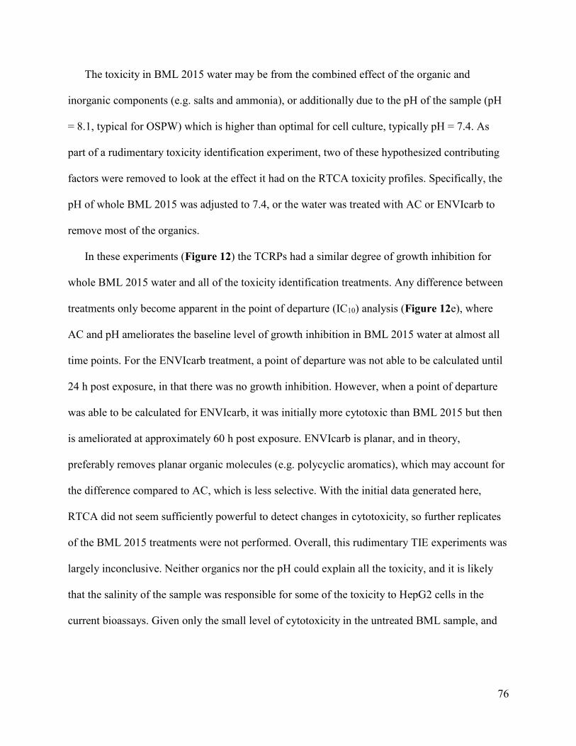
76

The toxicity in BML 2015 water may be from the combined effect of the organic and

inorganic components (e.g. salts and ammonia), or additionally due to the pH of the sample (pH

= 8.1, typical for OSPW) which is higher than optimal for cell culture, typically pH = 7.4. As

part of a rudimentary toxicity identification experiment, two of these hypothesized contributing

factors were removed to look at the effect it had on the RTCA toxicity profiles. Specifically, the

pH of whole BML 2015 was adjusted to 7.4, or the water was treated with AC or ENVIcarb to

remove most of the organics.

In these experiments (Figure 12) the TCRPs had a similar degree of growth inhibition for

whole BML 2015 water and all of the toxicity identification treatments. Any difference between

treatments only become apparent in the point of departure (IC10) analysis (Figure 12e), where

AC and pH ameliorates the baseline level of growth inhibition in BML 2015 water at almost all

time points. For the ENVIcarb treatment, a point of departure was not able to be calculated until

24 h post exposure, in that there was no growth inhibition. However, when a point of departure

was able to be calculated for ENVIcarb, it was initially more cytotoxic than BML 2015 but then

is ameliorated at approximately 60 h post exposure. ENVIcarb is planar, and in theory,

preferably removes planar organic molecules (e.g. polycyclic aromatics), which may account for

the difference compared to AC, which is less selective. With the initial data generated here,

RTCA did not seem sufficiently powerful to detect changes in cytotoxicity, so further replicates

of the BML 2015 treatments were not performed. Overall, this rudimentary TIE experiments was

largely inconclusive. Neither organics nor the pH could explain all the toxicity, and it is likely

that the salinity of the sample was responsible for some of the toxicity to HepG2 cells in the

current bioassays. Given only the small level of cytotoxicity in the untreated BML sample, and

77

possible interference by salts and other inorganics, this direct approach to toxicity testing of

OSPW was deemed ineffective.

Figure 12: Toxicity identification analysis with HepG2 cells and RTCA after exposure to a)

BML 2015 and its treatments: b) pH adjustment to 7.4, c) ENVIcarb treatment stripping the

organics, and d) Activated Carbon treatment also stripping the organics. Values are the mean ±

SEM (n = 4 replicates within a plate), indicating deviation for all treatments from negative

control (Neg Cont). In e), the point of departure, or IC10, is calculated across time points, where 0

h is the point of treatment. Only BML 2015 was tested in three plate replicates (mean ± SEM),

while the toxicity identification treatments overall did not appear sufficiently different to warrant

further replicates.

0 20 40 60 80 1000

1

2

3

4

5

6

7

Neg Cont

100%

80%

60%

Time (h)

No

rmalized

Cell In

dex

20%

40%

0 20 40 60 80 1000

1

2

3

4

5

6

7

Neg Cont

100%

80%

60%

Time (h)

No

rmalized

Cell In

dex

20%

40%

0 20 40 60 80 1000

1

2

3

4

5

6

7

Neg Cont

100%

80%

60%

Time (h)

No

rmalized

Cell In

dex

20%

40%

0 20 40 60 800

50

100

150

200

Time (h)

IC10 (

%B

ML

)

BML 2015

ENVIcarb

pH-adjusted

AC

0 20 40 60 80 1000

1

2

3

4

5

6

7

Neg Cont

100%

80%

60%

Time (h)

No

rmalized

Cell In

dex

20%

40%

a) b)

c) d)

e)

78

The large body of literature already attributing toxicity of OSPW to the organic mixture

warranted further investigation of toxicity attribution for the organic components in the current

bioassay.15,84,106,154 Such information may guide the safe remediation and release of OSPW in the

future, and the organics are the major concern for the regulators and the industry.

3.1.2. Solvent vehicle and quality control experiments

In order to test the organic extracts of OSPW by RTCA, the type and % of solvent first

needed to be tested with HepG2 cells. Many toxicity studies testing OSPW organic extracts use

ethanol as a solvent control.43,51,100 A range of doses of anhydrous ethanol (100% purity) were

tested to find thresholds of cytotoxicity to HepG2 cells. The percent of solvent needed to be

sufficiently high to dissolve the OSPW organics and deliver them to cell culture media, but low

enough not to induce cytotoxicity. Cytotoxicity became apparent at a dose of 1% v/v ethanol

(Figure 13c). A lower dose of 0.2% ethanol showed no apparent effect, whereas a slightly higher

dose of 0.3% ethanol showed some evidence for enhanced proliferation. Therefore, a final

ethanol solvent composition of 0.25% was chosen to maximize solubility of the extracts. In the

same experiment, two doses of As (III) were tested as positive controls for cytotoxicity, and 250

µM was selected for further experiments due to the rapid cell death induced at this dose (Figure

13a).

A blank TAE was then performed with Optima® LC/MS Water to test for background

toxicity that might be introduced from impurities or contamination during the extraction. There

was no cytotoxic effect from the extraction blank (Figure 13b). A relevant environmental water

sample from the Athabasca River was also tested for background toxicity, and was not cytotoxic

to HepG2 cells, even at doses up to 12.5× its field concentration (Figure 13a).

79

Figure 13: TCRP of HepG2 cells after treatment with the TAE of a) River 2017 and b) LC/MS

grade water, and with c) anhydrous ethanol (EtOH), and arsenite (As3). Values are the mean ±

SEM (n = 4 replicates within a plate),

80

3.1.3. Evaluating environmental TAEs of different ages by RTCA

Using TAEs of environmental OSPW samples of different ages, their relative cytotoxicity

was tested by RTCA with HepG2 cells. As described above, BML 2013 was the least aged

sample and had the highest gravimetric concentration of organics. Here, BML 2013 was the most

cytotoxic sample, displaying dose-response cytotoxicity between 1.75× and 12.5× enrichment

factors (Figure 14a). The SEM of 4 replicates at each dose were quite narrow, thereby allowing

visual inspection of significant differences between the doses, and more quantitative analysis

performed with IC50 and IC10 calculations. The 10× dose appeared to flat-line the cell growth

from time of exposure, whereas the 12.5× dose likely killed the HepG2 cells, indicated by NCI

falling below 1 and eventually falling to 0, similar to the As (III) positive control.

The toxicity and dose-response of BML 2015 (Figure 14b) was similar to BML 2013, but the

highest dose (12.5×) did not kill the cells, but caused cell growth to stop, suggesting it as slightly

less toxic than BML 2013. Notably, at the environmentally relevant 1× dose of BML 2015

organics, the SEM overlapped with the negative control, suggesting no significant differences at

this dose. This is consistent with the whole BML 2015 water toxicity identification analysis in

Figure 12, where removal of the organics marginally increased the point of departure value,

though there was not sufficient power to know if this effect was significant. BML 2017 was even

less cytotoxic than BML 2015 and BML 2013, with a steady dose-response leading to the highest

dose of 12.5× almost flat-lining cell growth, though proliferation was still possible (Figure 14c).

Pond 9 (2016) displayed a unique biphasic response compared to all the BML samples,

whereby after 24 h of exposure it was cytotoxic, but the cells appeared to recover with exposure

time to an asymptote by approximately 60 h (Figure 14d). Pond 9 (2016) had been aged 23 yrs

at the time of collection, and may predict what BML water could look like in the future.

81

Figure 14: TCRPs of HepG2 cells after exposure to the TAE of a) BML 2013, b) BML 2015, c)

BML 2017, and d) Pond 9 2016. Values are the mean ± SEM (n = 4 replicates in a plate).

To quantify and compare the different TCRPs for each sample, 50% inhibitory concentration

(IC50) histograms were made. IC50 is defined as the concentration of an inhibitor required to

reduce cell growth by half; lower IC50’s indicate a more potent inhibitor of cell growth. The

measured response for each dose in each sample was compared to the negative control at every

time point and averaged across three replicate plates to generate a SEM. In IC50 histograms, 0 h

is the point of treatment of environmental samples.

BML samples all demonstrated a decrease of the IC50 over exposure time (Figure 15), with

BML 2013 having the lowest value and therefore being the most potent. For BML, cytotoxicity

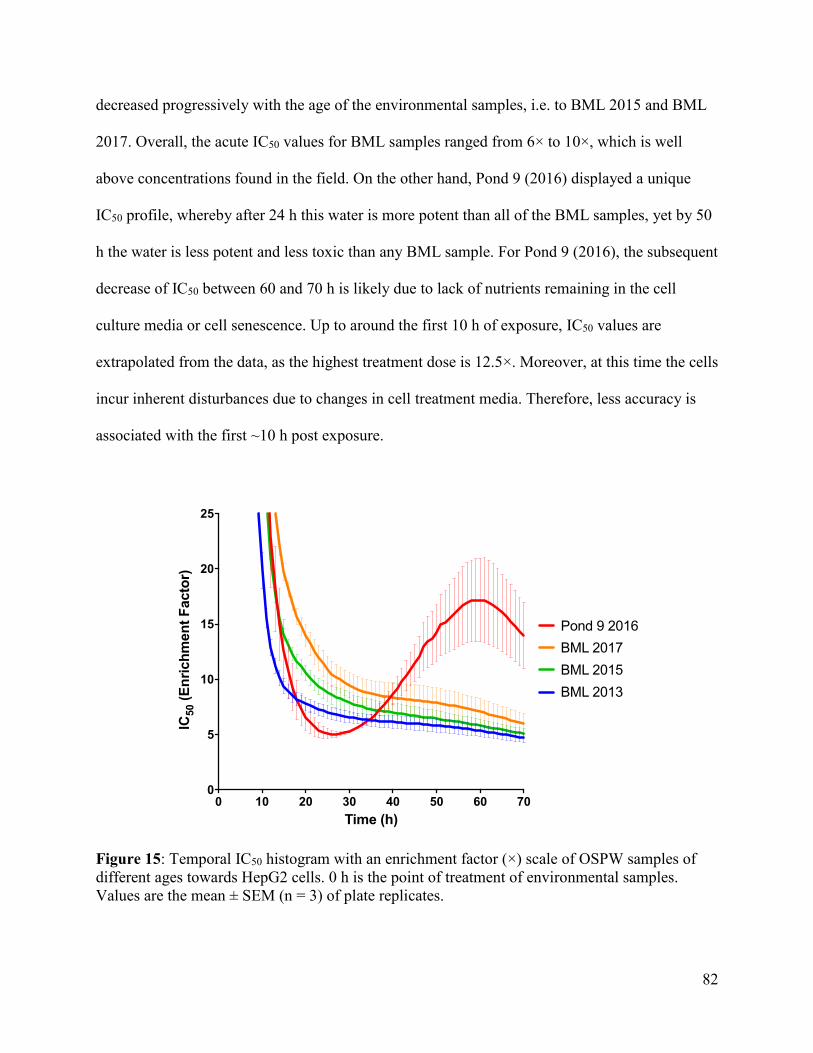
82

decreased progressively with the age of the environmental samples, i.e. to BML 2015 and BML

2017. Overall, the acute IC50 values for BML samples ranged from 6× to 10×, which is well

above concentrations found in the field. On the other hand, Pond 9 (2016) displayed a unique

IC50 profile, whereby after 24 h this water is more potent than all of the BML samples, yet by 50

h the water is less potent and less toxic than any BML sample. For Pond 9 (2016), the subsequent

decrease of IC50 between 60 and 70 h is likely due to lack of nutrients remaining in the cell

culture media or cell senescence. Up to around the first 10 h of exposure, IC50 values are

extrapolated from the data, as the highest treatment dose is 12.5×. Moreover, at this time the cells

incur inherent disturbances due to changes in cell treatment media. Therefore, less accuracy is

associated with the first ~10 h post exposure.

Figure 15: Temporal IC50 histogram with an enrichment factor (×) scale of OSPW samples of

different ages towards HepG2 cells. 0 h is the point of treatment of environmental samples.

Values are the mean ± SEM (n = 3) of plate replicates.

0 10 20 30 40 50 60 700

5

10

15

20

25

Time (h)

IC50 (

En

rich

men

t F

acto

r)

BML 2013

Pond 9 2016

BML 2017

BML 2015

83

While the enrichment factor-scale is an effective means at evaluating environmental

relevance of any toxic response (i.e. 1× is the concentration in the field), it is not useful for

benchmarking the absolute toxic potency, typically expressed as mass of substance per unit

volume (i.e. mg/L). Therefore, to compare the toxic potency of organics in each sample,

enrichment factor was transformed to mg/L based on the gravimetric concentrations (Table 7).

All differences in toxicity described above between BML 2013, BML 2015, and BML 2017

on the enrichment factor scale, disappear when plotted on the mg/L scale (Figure 16). In other

words, while the toxicity of the various BML water samples differs, the toxic potency of the

dissolved organics in each sample is identical. Pond 9 (2016) showed the same biphasic profile

after converting to mg/L, however the relative potency at 24 h is even more pronounced

compared to BML samples. Some IC50 (mg/L) values for Pond 9 (2016) after 60 h were not able

to be calculated by GraphPad (Figure 16), thus, all 3 replicates at that time were excluded.

Figure 16: Temporal IC50 histogram with mg/L scale for OSPW samples of different ages. 0 h is

the point of treatment of environmental samples. Values are the mean ± SEM (n = 3) of plate

replicates.

84

Given the result of the toxicity identification experiment with whole BML 2015 (Figure 12),

and the finding here that the SEM of the 1× dose of BML organics overlapped with negative

control, a more confirmatory point of departure, or IC10, analysis was performed, again, at each

time point for all BML TAE samples (Figure 17). In these experiments, the point of departure

approached but did not pass the field concentration of BML 2013 (75.8 mg/L), BML 2015 (66.0

mg/L), and BML 2017 (57.9 mg/L) after 100 h of exposure. However, it is important to note that

at 100 h of exposure other factors such as lack of nutrients in the 96-well plate or cell senescence

could contribute to an adverse effect, so IC values generally hold greater validity at earlier

exposure times, such as less than 80 h. No matter, overall this suggests a lack of effect of the

organics at 1×, and that only just above this point would a cytotoxic effect become observable.

Interestingly again, the point of departure is not changing with ageing of BML samples, further

supporting that toxic potency of the remaining organics is not changing (Figure 17).

85

Figure 17: Point of departure (IC10) over time of the TAEs of a) BML 2013, b) BML 2015, and

c) BML 2017, with their corresponding field concentration indicated by the dotted line. 0 h is the

point of treatment of environmental samples. Values are the mean ± SEM (n = 3) of plate

replicates.

0 20 40 60 80 1000

50

100

150

200

250

300

350

400

Time (h)

IC10 (

mg

/L)

Estimated

concentration

of BML 2013

TAE

0 20 40 60 80 1000

50

100

150

200

250

300

350

400

Time (h)

IC10 (

mg

/L)

Estimated

concentration

of BML 2015

TAE

0 20 40 60 80 1000

50

100

150

200

250

300

350

400

Time (h)

IC10 (

mg

/L)

Estimated

concentration

of BML 2017

TAE

a)

b)

c)

86

3.1.4. Attributing cytotoxicity by RTCA to certain chemical classes in BML 2015

The two fractions (F1, F2), along with the two washes (W1, W2) obtained through SPE

fractionation of BML 2015 were tested by RTCA in HepG2 cells to identify chemical classes of

concern. F1, containing predominantly NAs, was the most cytotoxic fraction, showing a clear

dose-response, and at the highest dose (12.5×) the cell growth flat-lined (Figure 18), similar to

unfractionated BML 2015 TAE (Figure 14b). The results for F2 and W1 were difficult to

interpret because of enhanced proliferation compared to negative control, possibly a stress

response in HepG2 cells, but evidence for cytotoxicity was generally lacking. W2 had a minor

cytotoxic response, but not enough for an IC50 to be calculated.

Figure 18: TCRPs of BML 2015 fractions in RTCA with HepG2 cells. a) F1 contains NAs and

was the most cytotoxic fraction, b) F2 contains largely polar non-acids, and c) W1 and d) W2 are

mixtures of chemical classes. Values are the mean ± SEM (n = 4 of replicates in a plate).

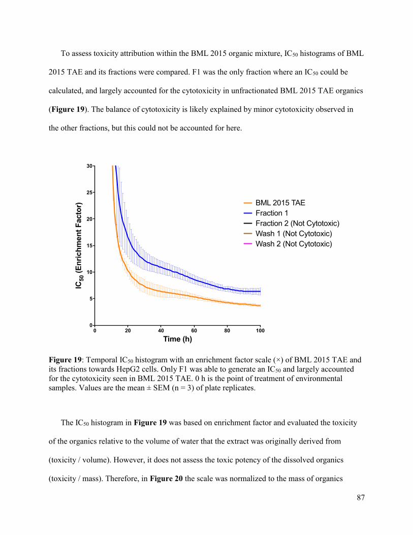
87

To assess toxicity attribution within the BML 2015 organic mixture, IC50 histograms of BML

2015 TAE and its fractions were compared. F1 was the only fraction where an IC50 could be

calculated, and largely accounted for the cytotoxicity in unfractionated BML 2015 TAE organics

(Figure 19). The balance of cytotoxicity is likely explained by minor cytotoxicity observed in

the other fractions, but this could not be accounted for here.

Figure 19: Temporal IC50 histogram with an enrichment factor scale (×) of BML 2015 TAE and

its fractions towards HepG2 cells. Only F1 was able to generate an IC50 and largely accounted

for the cytotoxicity seen in BML 2015 TAE. 0 h is the point of treatment of environmental

samples. Values are the mean ± SEM (n = 3) of plate replicates.

The IC50 histogram in Figure 19 was based on enrichment factor and evaluated the toxicity

of the organics relative to the volume of water that the extract was originally derived from

(toxicity / volume). However, it does not assess the toxic potency of the dissolved organics

(toxicity / mass). Therefore, in Figure 20 the scale was normalized to the mass of organics

0 20 40 60 80 1000

5

10

15

20

25

30

Time (h)

IC50 (

En

rich

men

t F

acto

r) BML 2015 TAE

Fraction 1

Fraction 2 (Not Cytotoxic)

Wash 2 (Not Cytotoxic)

Wash 1 (Not Cytotoxic)

88

(toxicity / mass), and this showed how F1 was evidently much more potent than BML 2015

TAE. This is sensible because the cytotoxic chemical class, NAs, is largely isolated from the rest

of the organics, which were shown to have lower cytotoxicity.

Figure 20: Temporal IC50 histogram on a mg/L scale of BML 2015 TAE and the cytotoxic

fraction, F1, towards HepG2 cells. Values are the mean ± SEM (n = 3) of plate replicates.

Given that F1 was by far the most cytotoxic fraction in BML 2015, the IC10 over time was

calculated as a rudimentary estimation of the point of departure (Figure 21). The IC10

approached the relevant field concentration of the F1 chemical classes in BML 2015 (12.9

mg/L), but came to a plateau at ~17 mg/L. This value will later be compared to the estimated

point of departure for sub-lethal endocrine activity. The point of departure toxicity profile of F1

is similar to that of BML 2015 TAE (Figure 17c).

0 10 20 30 40 50 60 70 80 90 1000

200

400

600

800

1000

1200

1400

1600

1800

2000

Time (h)

IC50 (

mg

/L)

Fraction 1

BML 2015 TAE

89

Figure 21: Point of departure over time for the F1 fraction by RTCA in HepG2 cells. Values are

the mean ± SEM (n = 3) of plate replicates, and the estimated field concentration of F1 is

indicated by the dotted line.

3.1. Yeast Estrogen and Androgen Screening (YES/YAS)

3.1.1. Attributing agonism and antagonism to BML 2015 fractions

Part of the YES/YAS assay incorporates a measurement of cytotoxicity (growth factor)

because it is important that non-cytotoxic doses are used for accurate interpretation of the

colorimetric response. Xenometrix sets growth factor criteria based on comparison of the optical

density in the sample relative to solvent control, with the ratio not to drop below 50%. Using the

YES antagonist experiment as an example (Figure 22a), F1 was cytotoxic at ~2×, F2 was

cytotoxic at ~10×, while W1 and W2 were not cytotoxic. Similarly, using the YAS antagonist

experiment as an example (Figure 22b), F1 was cytotoxic at doses greater than ~3×, F2 was not

cytotoxic below 12.5×, while W1 and W2 were not cytotoxic at any dose. Doses that lead to

cytotoxicity were excluded when measuring ER and AR interactions here.

0 20 40 60 80 1000

10

20

30

40

50

60

70

80

90

100

Time (h)

IC10 (

mg

/L)

Fraction 1

Estimated

concentration

of F1 in BML

2015

90

Figure 22: Growth during antagonist experiment after treatment with BML 2015 fractions for a)

YES and b) YAS strains. Plate reader measured OD690 after 18 h of exposure. 1.00 = the solvent

control growth factor. Values are the mean ± SEM (n = 2 in the plate). Cytotoxicity is

categorized by Xenometrix as when the growth factor is < 50% of the solvent control and this is

indicated by the dotted line at 0.50.

To identify receptor agonists in the YES/YAS assay, induction ratios were log transformed,

normalized (100% = max positive control induction ratio, 0% = solvent control), and a sigmoidal

dose-response curve was applied. The agonist criterion set by Xenometrix is that Induction >10%

0 1 2 3 4 5 6 7 8 9 10 11 12 130.00

0.25

0.50

0.75

1.00

1.25

1.50

1.75

Enrichment Factor (x)

Gro

wth

Facto

r

F1

F2

W1

W2

Qualifying

cut off

0 1 2 3 4 5 6 7 8 9 10 11 12 130.00

0.25

0.50

0.75

1.00

1.25

Enrichment Factor (x)

Gro

wth

Facto

r

F1

F2

W1

W2

Qualifying

cut off

a)

b)

91

is indicative of agonism; therefore, no estrogen or androgen agonists were detected in any BML

2015 fractions through YES (Figure 23a) or YAS strains (Figure 23b), respectively.

Figure 23: No agonists present in BML 2015 fractions in the a) YES or b) YAS strain.

Xenometrix criterion for agonism was indicated by the dashed line. Each treatment dose was run

in duplicate, though raw values were averaged earlier in the analysis process of the Xenometrix

workbook, not allowing for error to be carried through to the final figures.

To screen for antagonists, the assays are repeated with fixed concentrations of positive

control hormones, either E2 or DHT, in the test media of all wells. Positive results are indicated

-5 0-10

0

10

20

30

40

50

60

70

80

90

100

110

Log (mg/L)

Ind

ucti

on

%

F1

F2

W1

W2

E2

Qualifying

cut off

-4 -2 0 2 4-10

0

10

20

30

40

50

60

70

80

90

100

110

Log (mg/L)

Ind

ucti

on

%

F1

F2

W1

W2

DHT

Qualifying

cut off

a)

b)

92

by a decrease in Induction %, and the Xenometrix criterion for antagonism is when Induction is

less than 50%. As such, ER antagonists were present throughout all BML 2015 fractions (Figure

24a). The cytotoxic doses of F1 were excluded, leaving only three data points, which were too

few to generate a sigmoidal function, but the three available data points were nevertheless

formally indicative of ER antagonist. The highest dose of F2 was also removed due to

cytotoxicity, but the remaining lower doses were sub-lethal and allowed for the generation of a

sigmoidal function. W1 and W2 were less potent and were able to generate full dose-response

curves, with upper and lower plateaus starting to become observable (Figure 24a). This

suggesting that ER antagonists were present through the fractions at different potencies, with F1

and F2 being the most potent.

In the YAS assay, antagonists were also present throughout the BML 2015 fractions (Figure

24b). The highest doses of F1 were excluded because of cytotoxicity, but four non-cytotoxic

doses displayed antagonism and allowed for a sigmoidal function to be applied. Similar to the

YES antagonist experiment (Figure 24a), F1 and F2 were the most potent, with W1 and W2

lower in potency. However, W1 seems to have greater YAS antagonism than YES antagonism,

while W2 has YES antagonism, but barely passed the cut-off for YAS antagonism.

93

Figure 24: a) YES antagonists and b) YAS antagonists were present throughout BML 2015

fractions. Xenometrix’s criterion of antagonism is indicated by the dotted line (<50%). 4-HT was

a known antagonist of the ER, and FL was a known antagonist of the AR. Each treatment dose

was run in duplicate, though raw values were averaged earlier in the analysis process of the

provided Xenometrix workbook, not allowing for error to be carried through to the final figures.

-4 -3 -2 -1 0 1 2 3 40

10

20

30

40

50

60

70

80

90

100

110

Log (mg/L)

Ind

ucti

on

%F1

F2

W1

W2

4-HT

Qualifying

cut off

-3 -2 -1 0 1 2 30

10

20

30

40

50

60

70

80

90

100

110

Log (mg/L)

Ind

ucti

on

%

F1

F2

W1

W2

FL

Qualifying

cut off

a)

b)

94

In both YES and YAS, F1 and F2 appeared to be of similar potency to the positive control

hormones: 4-HT for ER antagonism and FL for AR antagonism (Figure 24). However, the

curves generated for all of the BML 2015 fractions were incomplete, with doses only revealing

the high-end of the dose-response relationship, particularly for the most bioactive fractions, F1

and F2. Therefore, quantitative analysis was held off until the YES and YAS antagonist assays

were run again at a wider and lower range of doses.

In the next trial, lessons learned were incorporated with a change in methodology, as defined

in section 2.8. Also, only antagonism was screened for, as there were no agonists found. The

maximum sub-lethal dose of F1 was 3×, while F2, W1, and W2 were able to go up to 10× and

still be sub-lethal. In this trial, complete dose-response curves were generated with upper and

lower plateaus, allowing for accurate EC50 measurements and for the data to be analyzed in both

a mg organics/L scale for toxic potency and an enrichment factor scale for environmental

relevance (Figure 25). On a mg/L scale, F1 and F2 were similar in potency and are both more

potent than the positive control hormones for YAS antagonism (Figure 25a) and YES

antagonism (Figure 25c). On an enrichment factor scale, F1 and F2 were more divergent in

terms of their YAS antagonism (Figure 25b) and YES antagonism (Figure 25d), with F1

becoming comparably slightly more potent, indicating greater environmental relevance. W1 and

W2 only have an effect at their highest doses and were both less potent than the positive control

antagonistic hormones (Figure 25a, c). W2 appears slightly more potent than W1 on a mg/L

scale, though it is of equal environmental relevance for YAS antagonism (Figure 25b). W1

appears more environmentally relevant than W2 for YES antagonism (Figure 25d).

95

Figure 25: Trial #2 of YAS antagonism on a) a mg/L scale and b) an enrichment factor scale, as

well as YES antagonism on c) a mg/L scale and d) an enrichment factor scale. Reduction % was

normalized to the antagonistic positive control for the assay, where 0% was the highest dose and

100% was the lowest dose. Only on the mg/L scale can the fractions be compared to the

antagonistic positive control of 4-HT for YES antagonism and FL for YAS antagonism. With the

new approach in analysis, values were the mean ± SEM (n = 2 replicates within a plate).

With the full dose-response curves generated, a quantitative approach could now be taken,

comparing the BML 2015 fraction EC50 and EC10 values to rank fractions in terms of potency, as

well as allow for comparison of the fractions to antagonistic positive control hormones to

determine equivalency (EQ). Here, an EQ value <1 means the sample was more potent than the

positive control hormone, and > 1 means the sample was less potent.

-3 -2 -1 0 1 2 30

25

50

75

100

125

150

Log (mg/L)

Red

ucti

on

%

F1

F2

W1

W2

FL

-4 -3 -2 -1 0 1 2 3-100

-50

0

50

100

150

Log (mg/L)

Red

ucti

on

%

F1

F2

W1

W2

4-HT

-4 -3 -2 -1 0 1 20

25

50

75

100

125

150

Log (Enrichment Factor)

Red

ucti

on

%

F1

F2

W1

W2

-4 -3 -2 -1 0 1 2-100

-50

0

50

100

150

Log (Enrichment Factor)

Red

ucti

on

%

F1

F2

W1

W2

a) b)

c) d)

96

However, there were issues with the EC50 calculations for the positive control antagonistic

hormones needed to calculate EQ. Even though the dilution scheme of the positive controls were

set by the company, in the first trial the lowest doses of the positive controls appeared to still be

potent inhibitors compared to negative control, i.e. ~50% induction (Figure 24). Moreover,

GraphPad was largely not able to calculate an accurate EC50 for the experimental 4-HT or FL

treatment in the first or second YES/YAS trials.

Fortunately, the Xenometrix Workbook provided a commonly fitted value for the

antagonistic hormone controls, in order to compare the experimental and theoretical values.

Given the challenges, I resorted to using a ‘theoretical 4-HT’ EC50 value and ‘theoretical FL’

EC50 value. This has an inherent limitation in that the theoretical values are not generated from

the same experimental conditions, but it is a start to allow for some comparison of toxic potency.

Interestingly, for FL, GraphPad was able to experimentally define its EC50 at 1.6 mg/L, which

was quite similar to the Xenometrix’s theoretical EC50 of 2.91 mg/L, so using the theoretical

values may not be too different from the experimental values. However, to remain consistent

between YES and YAS, both ‘theoretical EC50 values’ of 4-HT and FL were used to determine

equivalency (EQ) of the BML 2015 fractions.

With that said, EC50 values of the BML 2015 fractions from the second trial were compared

to their field concentrations in BML 2015 to assess environmental relevance and compared to

antagonistic control hormones to asses toxic potency (Table 8). F1, W1, and W2 were all more

potent YES antagonists than YAS antagonists based on their EC50 values, while F2 was

marginally a more potent YAS antagonist (Table 8). The YES and YAS antagonists were

distributed amongst all the fractions, indicating that the fractionation technique did not isolate the

endocrine active species into a single fraction. Without the vehicle control, categorizing these

97

samples as antagonist based on Xenometrix’s criteria (i.e. reducing the IR of max solvent –

vehicle control by 50%) was not possible (discussed in section 2.8), though compared to positive

antagonistic controls, it was clear that there was a similar antagonistic response.

More specifically, F2 was the most potent AR antagonist, with an EC50 of 2.04 mg/L, which

was slightly below its field concentration in BML 2015, and has a FL-EQ of 0.70 (Table 8). F1

was the most potent ER antagonist, with an EC50 of 0.11 mg/L, which was far below its field

concentration in BML 2015, and has a 4-HT EQ of 0.09 (Table 8). Overall, F1 and F2 were the

most potent and were the only fractions that had FL and 4-HT EQ values below 1, suggesting

successful isolation of the most potent chemical classes in these two fractions. W1 had an EC50

above BML 2015 field concentrations, though its EC10 was below (Table 8).

The point of departure for YES and YAS antagonism of F1, F2, and W1 are all far below

their estimated concentration, while W2 generated ambiguous values, suggesting less

environmental relevance (Table 8). With the degree of isolation and separation achieved in the

SPE fractionation, this allowed for generating novel toxicological information for particular

chemical classes, specifically: assigning a threshold for which ER or AR antagonists effects

begin to be detected below controls. F1 had a YES antagonism threshold of 0.019 mg/L and

YAS antagonism threshold of 0.36 mg/L, while F2 had an YES antagonism threshold of 0.043

mg/L and YAS antagonism threshold of 0.24 mg/L.

3.1.2. Evaluating ageing through antagonism of environmental TAEs

Lessons learned from the first YES/YAS trial with BML 2015 fractions were extended here,

with knowledge that no agonists were detected even in isolated fractions and that a wider and

lower dilution scheme is needed for sublethal doses. To ensure that the new environmental

98

samples tested were sublethal, an initial cytotoxicity test with the YES strain was run; the YES

strain was more sensitive than the YAS strain in the first trial (Figure 22). The new samples

tested were BML 2013, BML 2017, Pond 9 (2016), and River 2017. Here, a range of doses were

used to find the dose that decreased the growth factor of negative control by 50%, as set by

Xenometrix.

BML 2013 and BML 2017 had similar cytotoxicity, causing ~50% reduction in growth factor

at the dose of 5× after 18 h post exposure (Figure 26a). When tested with a longer exposure time

of 40 and 46 h though, yeast treated with the highest dose (10×) of BML 2017 recovered, while

yeast in BML 2013 did not (Figure 26b). Thus, BML 2013 was the most cytotoxic, and keeping

the highest dose of BML samples at or below 3× should be sufficient for assessing sub-lethal

effects in the YES/YAS antagonism assay. For Pond 9 (2016) and River 2017 there was minor

cytotoxicity that was very close to the negative control, even up to 10× and over prolonged time

as well (though River 2017 was not tested over time). Interestingly, while HepG2 cells treated

with Pond 9 (2016) was cytotoxic and had a biphasic response with prolonged exposure time by

RTCA (Figure 15), with yeast Pond 9 (2016) had a marginal effect, and the biphasic response

was observed in BML 2017 (Figure 26b).

In Figure 26a, the ethanol treatment contained the corresponding dose of solvent at each

dose of TAE, up to 0.67% in 10×. Therefore, ethanol did not affect yeast growth at any dose

tested here. Based on this initial cytotoxicity experiment, the maximum dose for the cytotoxic

samples (i.e. BML 2013 and BML 2017) was 3×, while for the non-cytotoxic samples (i.e. River

2017 and Pond 9 (2016)) it was 10×.

99

Figure 26: Growth of YES strain after treatments with TAEs of environmental samples a) over a

range of doses, and b) monitoring the 10× dose over time. Values are the mean ± SEM (n = 2

replicates in a plate).

In Figure 27, data were plotted by enrichment factor (×) in the right panel to rank samples by

environmentally relevant concentrations, and in the left panel the mg/L scale was used to

compare all treatments to antagonistic positive controls. In evaluating ageing as a remediation

strategy, the antagonistic effect of environmental OSPW samples of different ages were

0 1 2 3 4 5 6 7 8 9 10 110.00

0.25

0.50

0.75

1.00

1.25

Dose (x)

Gro

wth

Facto

r

1 yr aged

(BML 2013)

5 yrs aged

(BML 2017)

23 yrs aged

(P9 2016)

Reference

(AR 2017)

Ethanol

Qualifying

cut off

0 10 20 30 40 500.00

0.25

0.50

0.75

1.00

1.25

Time (hr)

Gro

wth

Facto

r

1 yr aged

(BML 2013)

5 yrs aged

(BML 2017)

23 yrs aged

(P9 2016)

Qualifying

cut off

a)

b)

100

contrasted. They were also compared to a reference sample of Athabasca River water, upstream

of the oil sands industry. In this trial, full dose-response curves were generated with upper and

lower plateaus (Figure 27). In both YES and YAS, there was a clear distinction between OSPW-

impacted samples and the reference River 2017 sample, in that OSPW-impacted samples had a

greater antagonistic effect and were effective at much lower doses (Figure 27). Secondly, on

both enrichment factor (×) and mg/L scales, there were hardly any differences in the YES and

YAS antagonistic effect between OSPW samples that were aged 1 year (BML 2013), 5 years

(BML 2017), or 23 years (Pond 9). As a reminder, all of these doses are sub-lethal, so the BML

samples had the highest dose of 1× (3× was excluded due to cytotoxicity), while Pond 9 went up

to 3× (10× was excluded due to cytotoxicity). Interestingly, when comparing Pond 9 (2016) at 1×

to the BML samples at 1×, Pond 9 (2016), even as the oldest sample, had the highest efficacy for

YES antagonism (Figure 27d).

101

Figure 27: YAS antagonism on a) a mg/L scale and b) enrichment factor scale, as well as YES

antagonism on c) a mg/L scale and d) enrichment factor scale. Reduction % was normalized to

the antagonistic positive control for the assay, where 0% was the highest dose and 100% was the

lowest dose. Only on the mg/L scale can the TAEs be compared to the positive control hormone

of 4-HT for YES antagonism and FL for YAS antagonism. With the new approach in analysis,

values were the mean ± SEM (n = 2 replicates in a plate).

While there were marginal differences among OSPW-impacted samples visually, quantitative

calculations allowed for the ranking of potency (mg/L). For YES antagonism, the high to low

potency decreased as follows: F1, F2, BML 2017, Pond 9 (2016), BML 2013, W2, W1, and

River 2017 (Table 8). For YAS antagonism, the high to low potency decreased as follows: F2,

F1, BML 2017, BML 2013, W2, Pond 9 (2016) = W1, and River 2017 (Table 8). It was

-4 -3 -2 -1 0 1 2 3-100

-50

0

50

100

150

Log (mg/L)

Red

ucti

on

%

1 yr aged

(BML 2013)

5 yrs aged

(BML 2017)

23 yrs aged

(P9 2016)

Reference

(AR 2017)

4-HT

-3 -2 -1 0 1 2 30

25

50

75

100

125

150

Log (mg/L)

Red

ucti

on

%

1 yr aged

(BML 2013)

5 yrs aged

(BML 2017)

23 yrs aged

(P9 2016)

Reference

(AR 2017)

FL

-4 -3 -2 -1 0 1 20

25

50

75

100

125

150

Log (Enrichment Factor)

Red

ucti

on

%

1 yr aged

(BML 2013)

5 yrs aged

(BML 2017)

23 yrs aged

(P9 2016)

Reference

(AR 2017)

-4 -3 -2 -1 0 1 2-100

-50

0

50

100

150

Log (Enrichment Factor)

Red

ucti

on

%

1 yr aged (BML 2013)

5 yrs aged

(BML 2017)

23 yrs aged

(P9 2016)

Reference

(AR 2017)

a) b)

c) d)

102

interesting that BML 2017 was consistently more potent than BML 2013, and also that the

endocrine active fractions, F1 and F2, were consistently more potent than the OSPW TAEs.

Even though there was minor variability between the BML and Pond 9 samples, the EC50 values

overall were quite similar, which is surprising considering the amount of ageing between

samples and the differences in chemical profiles (Figure 9). Also, all of the River 2017

calculations were ambiguous and far above field concentrations, showing a clear divergence in

effect for all OSPW-impacted samples.

More specifically, the EC50 values for ER and AR antagonism of BML 2013, BML 2017, and

Pond 9 (2016) were all below their field concentrations (Table 8). As discussed, the

experimental 4-HT and FL EC50 values were largely ambiguous again, so the theoretical EC50

values were taken from Xenometrix’s workbook to determine equivalence (EQ). Here, BML

2017 and Pond 9 (2016) were both more potent on a mg/L scale than 4-HT, indicated by EQ

values below 1, while BML 2013 had a 4-HT of 1.01. For YAS antagonism, none of the TAEs

were below 1 for FL EQ equivalence, and only the BML 2015 fractions, F1 and F2, were below

1. Overall, this highlights isolation of the most potent chemical classes in F1 and F2 for YAS

antagonism, as well as for YES antagonism, though the potency of TAEs of OSPW-impacted

samples are close behind. The points of departure were based on EC10 estimations, and

considering that all of the OSPW-impacted samples had EC50’s below field concentrations, their

corresponding EC10’s were also all below field concentrations (Table 8).

103

Table 8: Quantifying the antagonistic potency of BML 2015 fractions and environmental sample TAEs by YES/YAS.

Note: Field [ ] is an estimation of field concentration by gravimetric analysis. Anti-YES is YES antagonism, and Anti-YAS is YAS

antagonism. ‘~’ indicates an ambiguous measurement. F1, F2, W1, W2 were fractions of BML 2015, while BML, Pond 9, and River

samples were TAEs. EC50’s and EC10’s (the point of departure measurement) were based on gravimetric analysis (mg/L). 4-HT and

FL were known antagonistic chemicals, to which their theoretical EC50’s were compared to experimental treatments to derive an

equivalency value (EQ), where a ratio less than 1 was indicative of greater potency than the given antagonistic chemical.

Field [ ]

mg/L

Anti-YES EC50 mg/L

Anti-YES EC10 mg/L

EC50 Below field [ ]

4-HT EQ based on

Anti-YES EC50

Anti-YAS EC50 mg/L

Anti-YAS EC10 mg/L

EC50 Below field [ ]

FL EQ based on Anti-YAS

EC50

F1 12.9 0.11 0.019 yes 0.09 2.61 0.36 yes 0.90

F2 2.10 0.26 0.043 yes 0.21 2.04 0.24 yes 0.70

W1 21.8 25.1 2.19 20.5 370 27.8 127

W2 1.70 10.3 ~5.29e3 8.42 17.2 ~3.04e5 5.92

BML 2013

75.8 1.24 0.049 yes 1.01 16.2 2.06 yes 5.58

BML 2017

57.9 0.33 0.14 yes 0.27 11.8 1.70 yes 4.05

Pond 9 (2016)

38.1 0.83 0.26 yes 0.67 17.2 2.46 yes 5.92

River 2017

0.76 ~198 ~3.39e3 161 ~3.81e4 1.80 1.22e4

4-HT 1.23 1.00

FL 2.91 1.00

104

4. Discussion

4.1. Toxicity attribution for BML 2015

4.1.1. Cytotoxicity of whole BML 2015

With acute mammalian LD50 assays banned in 2002 by the OECD,155 alternative means to

assess relevant mammalian toxicity and mechanisms of action are necessary, and much of the

past toxicity testing of OSPW has focused on aquatic organisms, which is still allowed by the

OECD. There is an urgency to move towards more in vitro toxicity testing and away from in vivo

lethality testing as part of the modern toxicology ‘3R framework’ of replacement, reduction, and

refinement.125 Although common regulatory ecotoxicology assays for industrial effluents may

not yet be replaceable - such as the 96 h acute lethality test in fish - in vitro tests may be

advantageous for prioritizing contaminants in high-throughput formats, differentiating between

mechanisms of action with less subjective apical endpoints, and being more rapid and less

expensive.29 RTCA is valuable technology for assessing human cellular toxicity of mixtures in

environmental water samples of relevance to human exposure.

To further advance our understanding of chemicals that attribute toxicity to the sample of

BML from 2015, HepG2 cells were tested using RTCA. The samples tested included: whole

BML 2015 water, whole BML 2015 water treated by adsorption with AC or ENVIcarb, or whole

BML 2015 water with a pH adjustment, as well as BML 2015 TAE, an extraction control, and a

reference natural water sample.

A 100% dose of whole BML 2015 water was not cytotoxic enough to generate an IC50 with

HepG2 (Figure 11). However, an IC10 point of departure analysis demonstrated that a cytotoxic

effect started to surface at approximately 50% BML 2015 water, and this remained consistent

105

from 20-80 h post exposure, indicating minor toxicity (Figure 12e). Through IC10 comparisons,

toxicity was marginally reduced after treatment with ENVIcarb, AC, and by pH-adjustment,

though this reduction did not appear statistically or biologically significant (Figure 12e).

Therefore, under these conditions the organic content, the elevated pH, and high concentration of

salts typical of all OSPW could not be delineated. However, the combined effect of a powdered

media (EMEM), formulated with the optimal osmolarity for HepG2 growth, with the addition of

a high salt and high pH OSPW sample as the reconstituting agent, may lead to hyperosmotic

conditions and sub-optimal cell proliferation. Ultimately, with only a minor toxic effect of BML

2015, and no practical way to concentrate it without also increasing salt concentrations, the

approach of testing whole OSPW by RTCA was deemed too insensitive and inappropriate to

meet the objectives of the research in this thesis.

A previous study reported that the inorganic components of OSPW at field concentrations in

an active Syncrude tailings pond, Aurora, was cytotoxic and immunotoxic to mammalian

macrophages.109 They argued that the effect was not due to the saltiness of OSPW, because its

osmolarity was actually less than that of the cell culture media; however, they did not rule-out

effects from osmolarity. Importantly, this study used a different experimental approach for

exposing the cells than in the current work. Liquid media with a natural osmolarity was used

with liquid OSPW added to it, and a corresponding control containing the amount of volume

displaced by OSPW but with phosphate-buffered saline (PBS).109 Here, powdered media

(containing optimal salts for HepG2) was reconstituted with 100% aqueous OSPW (instead of

pure water). Thus, the final osmolarity exceeded the optimal conditions for HepG2, possibly

causing some toxicity. However, with this method a 100% dose of OSPW was accomplished,

enabling a point of departure calculation.

106

Due to difficulties working with whole OSPW, the next step in the toxicity identification

approach was to extract the organic mixture to assess and test its toxicity without the

confounding effects of inorganics and salts, thereby minimizing any osmolarity-related effects.

Notably, when testing the TAE of BML 2015, the 1× dose did not significantly reduce cell

growth compared to negative control (Figure 14), which was further evidence that the organics

did not contribute to the minor toxicity in 100% whole BML 2015. Furthermore, the calculations

in Figure 17 showed how the point of departure approached the estimated field concentration of

BML 2015 (66 mg/L) by 100 h post exposure, though it did not go beyond. Overall, this

confirms the initial suspicions that the organic mixture in whole BML 2015 is not responsible for

the growth inhibition observed in whole BML 2015. This is also in line with Syncrude Canada

Ltd.’s data of BML (Table 3), where the whole effluent (100%) from 2016 was generally not

toxic in various acute toxicity assays. A caveat of the point of departure calculation in Figure 17

is that at 100 h post exposure there may be inherent toxicity due to lack of nutrients in wells and

natural cell senescence, whereas the more accurate data is taken between ~10-72 hours post

exposure. Nevertheless, even at the 72 h time point, the conclusion is maintained that the point of

departure exceeds, but approaches, the field concentrations of all BML samples.

Further exploring the dose-response of BML 2015 TAE, cytotoxicity was in fact detected

near the 1.75× dose and steadily became more potent up to 12.5×, at which point cell growth was

flat-lined immediately from the time of exposure (Figure 14b). The extraction control (TAE of 1

L of LC/MS water) demonstrated that the extraction process itself did not introduce

contamination to alter cell proliferation (Figure 13b). Similarly, the 1 L TAE of an upstream

Athabasca River water did not demonstrate any cytotoxicity (Figure 13a). Overall, this indicated

that the bitumen-derived organics generated and concentrated through industrial processing were

107

responsible for the cytotoxicity observed in BML 2015 TAE. This is a novel finding considering

the lack of human-relevant cytotoxicity data, especially with RTCA, which measures cell

morphology, growth, and proliferation through a more holistic lens compared to colorimetric

assays that have specific endpoints dependent on specific processes, like metabolism.

BML 2015 TAE had IC50 values over time ranging from 6× to 9× above field concentrations,

depending on exposure time (Figure 15). Notably, Syncrude’s acute toxicity data (Table 3) were

ambiguous in stating that BML 2016 water had an IC50 >100%, therefore, these IC50 values

(Figure 15), albeit in human cells, give new insight and data that may be used as a benchmark

for monitoring remediation progress as BML ages.

Considering other literature, Sansom et al.29 tested 49 OSPW effluents at an 80% dose (i.e.

0.8×) to 6 fish cell lines and reported a high variability in cytotoxicity depending on tested

sample location, age, and treatment. Some of the OSPW samples decreased cell viability up to

90%, while others had no effect. Therefore, while here the organics at 1× did not cause an effect,

experimental parameters like species used in a bioassay and type of OSPW sample or extract can

have a big impact on the cytotoxic response.

For example, He et al.6 tested whole OSPW from WIP 2007, an activate tailings pond at the

time, on H295R human adrenocarcinoma cells (used for testing steroidogenesis) and found no

cytotoxicity with the MTT assay. This is interesting considering that WIP 2007 was an active

tailings pond and would be expected to be more concentrated and more potent than whole BML

2015 that has been aged and diluted. Garcia-Garcia et al.102 tested a NA-specific extract from

WIP 2006, with doses ranging from 6.25-50 mg/L NAs, where field concentration was 39.1

mg/L, and used 3 colorimetric cell assays on mouse bone marrow derived macrophages. Similar

to He et al.,6 they also did not find that cell viability was affected (i.e. with MTT or Trypan blue),

108

however, they reported that cell proliferation (BrdU assay) decreased by 40% (though not

statistically significant) when dosed with 50 mg/L NAs. Considering the NA concentration in the

BML 2015 sample used here was estimated to be 12.9 mg NAs/L (Table 6), achieving a 50

mg/L dose would require a 3.9× increase from field concentrations. Looking at the profile of

BML 2015 TAE (Figure 14) it could be estimated that a 3.9× dose may be close to a 40%

decrease in HepG2 proliferation. However, the nuances between studies may speak to the

differences in the endpoints measured in the colorimetric MTT assay, Trypan blue, or BrdU

proliferation assay, especially when compared to the impedance-based RTCA system, which

measures cell growth more holistically and with repeated measurements over time.

Further nuancing the discussion, Fu et al.109 used a scanning electron microscope to image

mouse macrophages treated with whole OSPW at environmentally relevant doses, and the treated

cells “featured frayed plasma membrane with multiple intrusive-like structure that are indicative

of membrane degeneration or/or disruption of membrane stability.” They go on to suggest

oxidative stress damage due to particular gene responses. However, when they tested the organic

fraction of OSPW alone, there were no changes in cell morphology, suggesting the effect was

from the combination of the inorganic fraction with the organic fraction.

Overall, there were conflicting results. Attempts to reconcile these differences and a possible

mechanism of action will be discussed later (section 4.2.3.1). However, it is important to note

that there may be multiple mechanisms contributing to cytotoxicity, and this may depend on the

source of OSPW, the dose at which the organics have their effect, and whether or not the

organics are in their original OSPW matrix.

109

4.1.2. Cytotoxicity of BML 2015 fractions

Based on Figure 7, BML 2015 organics were successfully fractionated using a SPE method

to re-create the most toxic fractions (i.e. NAs, and polar non-acids) based on the work of

Morandi et al.51 While Morandi et al.51 used BML 2012, here BML 2015 was studied; thus, there

has been three more years of potential biodegradation or other losses, with approximately 20% of

free water was added,8 as well as large doses of coagulating agents.144

In this study, fraction F1, which largely isolated the NA chemical class, had a calculated field

concentration of 12.9 mg/L and IC50 values with HepG2 cells ranging from 7× to 10× depending

on the exposure time, i.e. 24 - 100 h. Fractions F2 and W1 marginally enhanced cell

proliferation, likely as a stress response. W2 had marginal cytotoxicity, though an IC50 could not

be calculated. Therefore, the cytotoxicity of BML 2015 TAE was largely due to NAs (Figure

19). This is consistent with Morandi et al.,51 amongst other studies.55

Interestingly, when assessing toxic potency of the remaining organics on a mg/L scale, F1

was much more potent than the BML 2015 TAE (Figure 20). This is because NAs only account

for 20% of the TAE in terms of mass, and speaks to the successful isolation of the most acutely

toxic class in the fractionation method. This result is similar to Morandi et al.51 where their NA

fraction contained only 10.8% of the original dissolved organic mass.

The degree of isolation and separation of NAs from the rest of the chemical classes,

demonstrated in both positive and negative mode, allowed for a more accurate assignment of a

point of departure value to NAs. The point of departure of F1, largely composed of NAs,

approached their estimated field concentration in BML 2015 at 100 h post exposure, i.e. an IC10

of ~17 mg/L versus an estimated concentration of 12.9 mg/L in BML 2015 (Figure 21).

8 Personal communication with Warren Zubot, Syncrude Canada Ltd.

110

Furthermore, the point of departure for a cytotoxic effect of BML 2015 TAE (63 mg/L, Figure

17) also approached its estimated field concentrations (66 mg/L) at 100 h post exposure,

highlighting how the majority of the cytotoxicity can be attributed to NAs in the TAE. Therefore,

at only slightly above field NA doses in BML 2015 would a dissolved organic-driven toxic effect

be observed in a short-term test.

Fu et al.109 tested whole OSPW from the Aurora tailings pond (2014) with the RAW 264.7

mouse macrophage cell line. They exposed the cells for 18 h with additional OSPW acid

extractable organics added to whole OSPW, based on environmentally relevant NA

concentrations ranging up to 18 mg/L. When 12-18 mg/L NAs were added with the inorganic

content of OSPW, they were cytotoxic to the cells, reducing cell proliferation to less than 20% of

negative control in the BrdU test. Interestingly, this effect only occurred when the organics were

in the matrix of whole OSPW and not when the organics were isolated by themselves, nor when

whole OSPW had 0 mg/L NAs added. This finding was suggested to be due to a mixture effect

from the combination of organic and inorganics, and that when the organics are in their aqueous

matrix, NAs have a lower threshold for an effect than originally thought (12-18 mg/L).109

By comparison, the point of departure of NAs in this thesis approached 17 mg/L after 100 h

of exposure, though in Fu et al.,109 the point of departure was only ~70 mg/L at 18 h (Figure 21).

Despite the different exposure times, which may be determined by the intrinsic parameters of the

bioassay, only above 17 mg/L would NAs reach their threshold for a toxic effect. At 18 mg/L

NAs and only when within a whole OSPW matrix, Fu et al.109 observed reduced cell

proliferation (i.e. 0%) and reduced cell viability (i.e. <10%). This highlights that inorganics have

a profound effect on toxicity. Though, mammalian macrophages in vitro are outside of its host

organism and would not normally need to regulate their ion gradients to environmental

111

conditions outside of the host organism. Therefore, it is sensible for mammalian cells to be more

impacted by the inorganic content of OSPW, and this finding does not negate the pursuit of the

organics as a toxic component. Moreover, BML 2015 in the current study has been aged three

years and diluted with fresh water compared to fresh OSPW, so it is also sensible for this sample

to be less toxic than the Aurora active tailings pond. Though, to apply their conclusion of

mixture effects between the organic and inorganic fraction to this study, it would be interesting

to see if the point of departure of 17 mg/L NAs (above the estimated field concentration of 12.9

mg/L) here would be potentiated if tested within a whole BML 2015 matrix.

Looking at the F2 fraction, it is interesting that it was not acutely toxic to HepG2 cells even

at its highest doses of 12.5×. This is because Morandi et al.51 found their F2 fraction, containing

similar polar non-acids, was the second most acutely toxic fraction, resulting in 100% mortality

of fathead minnow embryos at ~5×. To potentially explain this difference, Morandi et al.51 used a

sample of BML from 2012 while the current study used BML from 2015, and the total intensity

of the species detected is known to have decreased with ageing (Figure 8); although the positive

mode species signal intensity appeared to deplete to a lesser extent than the negative mode

species. An alternative explanation could be that HepG2 cells have a different sensitivity to

OSPW organics compared to developing fathead minnow embryos, or that there are intrinsic

differences in the assays. The fractionation techniques used were similar in the purpose, yet

different in methodology, so the particular chemical classes isolated may also be somewhat

different. Interestingly, with testing the cytotoxicity of BML 2015 fractions on yeast, the

sensitivities to the BML 2015 fractions changed again: F1 was classified as cytotoxic based on a

reduction in growth factor beyond 50% at 2.5×, and F2 was classified as cytotoxic at 10×

112

(Figure 22). Therefore, there may be a combination of factors that lead to the differences

between Morandi et al.51 and the current study’s results.

On the other hand, Hughes et al.156 critiqued Morandi et al.51 and argued that the polar non-

acids were not relevant and that focus should still remain on classic NAs. They defended this

argument by saying that there is currently no way to quantify the positive mode species, and that

with an LC50 of 2.2× in Morandi et al,51 polar non-acids would result in minimal adverse effects

at field concentrations due to its relatively low potency compared to NAs, which had a reported

LC50 of 0.7×. However, just because a contaminant class cannot be quantified does not make it

toxicologically irrelevant. Secondly, I argue that an LC50 of 2.2× is indeed toxicologically

relevant due to the fact that this was an acute toxicity test, and the EPL strategy inherently

involves chronic exposure, and it is not clear which chemical classes may be most important in

longer term exposures. Moreover, Morandi et al.51 suggested that the polar non-acids may act

through a different mechanism than NAs, possibly endocrine disruption—in which case, sub-

lethal endpoints need also be assessed to prevent ecotoxicity.

Hughes et al.157 tested the toxicity of multiple organic fractions where the % composition of

classic NAs differed, and argued that the potency of individual NAs increased with carbon

number. They concluded this by finding that two fractions each had the same concentration of

NAs, though one fraction had 50% mortality, while the other had 100% mortality, and suggested

that the latter fraction had more potent NAs chemical species. However, they only analyzed their

samples in negative ion mode, so it is unknown whether positive mode species had an influence

on the observed toxicities of any of their fractions. While the current study indicated the polar

non-acids were even less acutely toxic than the Morandi et al.51 findings with fathead minnow

113

embryos, i.e. supportive of Hughes’ et al.156 argument, the sub-lethal effects of these non-acid

chemical classes still warrants testing, particularly with endocrine disruptive endpoints.

Despite differing opinions about relevance of the polar non-acids, the RTCA results in the

current study continue to support NAs as being the most acutely toxic chemical class in OSPW.

The human-relevant point of departure for NAs could contribute to the monitoring and regulating

of OSPW as it ages, in that a value of less than 17 mg/L is needed to not be acutely toxic to

human cells. That being said, this aspect of the study only tested RTCA with HepG2 cells, so the

point of departure conclusion cannot be made without a greater body of research and a species

sensitivity distribution. Nevertheless, this may be a useful starting point for determining other

human-relevant points of departure for NAs.

4.1.3. Endocrine activity of BML 2015 fractions

All of the BML 2015 fractions demonstrated anti-estrogenic and anti-androgenic effects, yet

none had any agonistic effects. I was successful in isolating the most cytotoxic chemical class,

the NAs, but the ER and AR antagonists were unexpectedly distributed throughout the fractions

with different potencies, though the majority of the effect was attributed to F1 and F2. In other

words, the endocrine active chemicals could not be isolated by chemical class alone, and other

fractionation approaches are warranted.

In the first YES/YAS trial, the polar non-acids in F2 were the most potent chemical classes,

however, the dose-response curves for most fractions were incomplete, leaving overall results

inconclusive. In the second YES/YAS trial with a wider and lower dose range, it became clear

through the full dose-response curves that F1 and F2 were similar in their antagonistic ability of

the ER and AR. Most interesting though, was that polar non-acids, while not being cytotoxic to

114

HepG2 cells and only marginally cytotoxic to yeast cells at high doses, were similarly potent (i.e.

mg/L scale) as NAs through a sublethal endocrine active mechanism of action. As discussed in

the section above, this must be considered in the overall discussion of environmental relevance

of various chemical classes compared to NAs. Nevertheless, on the × scale, F2 was in fact

slightly less environmentally relevant than F1. No matter, it is interesting that the EC50’s of

ER/AR antagonism for F1 and F2 were both below their estimated environmentally relevant

concentrations. F1 was the most acutely toxic fraction yet also had a potent sublethal

antagonistic ER/AR mechanism. With the very low doses of F1 and F2 needed in order to

generate an upper plateau on the dose-response (similar to the agonist baseline control, i.e.

negative control), this is consistent with the EC50 being drastically below environmentally

relevant concentrations. Overall, our hypothesis of F1 and F2 having different mechanisms was

not supported, however, even more concerning is that both of these fractions were endocrine

active through both ER and AR antagonistic mechanisms.

To characterize these fractions further, the point of departure threshold for toxic effects were

calculated. Since F1 and F2 were the most potent and relevant fractions, this novel threshold

could be useful in the absence of other data for interpreting targeted water monitoring and

remediation to ensure environmental protection. Based on the data generated here, F1, which is

largely the NA class, had an ER antagonism threshold of 0.019 mg/L, an AR antagonism

threshold of 0.36 mg/L, and a cytotoxic threshold of ~17 mg/L. Therefore, the sub-lethal effects

can be detected at a much lower dose than the cytotoxic effects, albeit in different assays with

different species. The ER/AR antagonism thresholds for F1 are quite potent, given the

concentration of 12.9 mg/L in BML 2015. However, a caveat should be noted that there is

uncertainty pertaining to the efficacy of the YES/YAS results, in that the results are scaled to the

115

positive control antagonistic hormone and not to the vehicle control. Notably, the point of

departures generated here are specific to these experiments, and a species sensitivity distribution

would be needed before implementation in any remediation strategy, as YES/YAS is only a

screening test.

F2 has an ER antagonism threshold of 0.26 mg/L and an AR antagonism threshold of 0.24

mg/L (i.e. more potent than F1). It was not cytotoxic to HepG2 cells, yet it was cytotoxic to yeast

at a dose of 10×. The estimated field concentration in BML 2015 is 2.10 mg/L; therefore, there is

less of a difference between the current concentrations of polar non-acids in BML and the point

of departure, while there is a bigger difference for F1. Therefore, reducing F2 to levels below its

point of departure would be more achievable than F1 for targeted remediation.

W1 and W2 both had measurable EC50’s, but for W2 an EC10 could not be calculated. This

could mean that W1 has a clearer dose-response for antagonistic effects and at more

environmentally relevant concentrations. Importantly, W2 had a lower concentration (1.70 mg/L)

than W1 and required a very high enrichment factor for antagonistic effects to surface, which is

not environmentally relevant. W1 had an EC50 above field concentrations in BML 2015, though

its EC10 is in fact below BML field concentrations, suggesting that it may too have relevance for

endocrine activity, in addition to F1 and F2. Therefore, chemical features other than molecular

formula class may be important in determining the endocrine activity of OSPW organics.

4-HT and FL equivalencies were calculated by comparing the EC50 values of environmental

samples with theoretical EC50 values of the known antagonistic hormones on a mg/L scale.

These equivalency values give insight to the potency of environmental samples compared to

known antagonists. On a mg/L scale, F1 and F2 were more potent than FL and 4-HT, while W1

116

and W2 were less potent (Table 8). Though it is important to emphasis that this is highlighting

mechanistic potency in an in vitro screen and is not linked to apical adverse effects.

Comparing the toxicity results with the Orbitrap MS results allows some extent of toxicity

attribution, though more work is needed. Among the least potent fractions, W1 contained a

mixture of chemical classes (O3-, O4

-, O2+, O3

+, SO3+, NO4

+) and while it was not cytotoxic in

RTCA, it had ER/AR antagonistic potencies at environmentally relevant doses. W2 contained

another mixture of chemical classes (O2-, O2

+, O3+, SO3

+, NO4+) in low abundance, had minor

cytotoxicity in RTCA, and while it did have ER/AR antagonist activity, these may only surface

at non-relevant environmental doses.

Considering the mixture of overlapping chemical classes between W1 and W2, this may

warrant a principle component analysis (PCA) to further attribute toxicity not only to fractions,

which still contain a mixture of chemical classes, but to unique chemical classes within the

fractions. Through a PCA, the intensity of a particular chemical class among all fractions could

be related to a given toxic effect. For example, W2 had minor cytotoxicity and contained O2- as

one of its prominent chemical classes, among others, while W1 was not cytotoxic and did not

contain O2- though was prominent in positive mode species. This may further support O2

- as

being the most cytotoxic class, while the positive mode species in W1 may be responsible for

maintaining the ER/AR antagonism, though a PCA could attempt to confirm this.

The toxicity attribution that has been suggested here should be compared to what already

exists in the literature. Yue et al.71 used the YES assay and Orbitrap analysis in negative mode

with OSPW from WIP, an active tailings pond. They suggested that O2-, O3

- and O4- species from

C17 to C20 with double bond equivalents between 6 and 10 had chemical formulas similar to

estrone-like and estradiol-like compounds. This is not consistent with the current data in that

117

YES agonists were not detected in the BML 2015 fractions, only YES antagonists. Notably, Yue

et al.71 did not analyze in positive mode, nor did they test for YES antagonism. However, there

may be chemicals in fresh OSPW, such as WIP, that are agonists but that degrade with ageing:

this hypothesis will be discussed in terms of antagonism (not agonism) in section 4.2.4.

Leclaire et al.70 tested OSPW aged 17 yrs using both YES and YAS and only found anti-

estrogenic and anti-androgenic effects; however, their extraction method was specific to NAs

and they only analyzed the extract in negative mode MS. Therefore, this is consistent with the

current investigation in that F1, largely containing NAs, did have YES/YAS antagonism and no

associated agonism. Leclaire et al.70 generated 4 fractions with different NA contents: fractions

with a higher aliphatic NA content appeared to be the most potent, with all fractions having

EC50‘s (mg/L) ranging from 1.5 - 16 mg/L for AR antagonism. In the current investigation, the

AR antagonism EC50 for a broader group of NAs was 2.61 mg/L (Table 8). Similarly in Leclaire

et al.,70 all of the fractions generated EC50’s (mg/L) ranging from 0.49 - 9.57 for ER antagonism,

while here, the EC50 for NAs was 0.11 mg/L. The main conclusion of Leclaire et al.70 was that

NAs can act through a steroid antagonism mechanism at environmentally relevant

concentrations. By extension, this investigation demonstrated that the polar non-acids and NAs

are both potent antagonists at environmentally relevant concentrations, with other chemical

classes potentially playing a role. A caveat in comparing studies are the different OSPW samples

and extraction techniques used. This highlights the importance of looking at endocrine activity

and cytotoxicity of different OSPW samples (section 4.2.4) with the same extraction method and

MS specifications.

The knowledge about mechanisms of action from in vitro studies could give insight into in

vivo observations. For example, evidence exists of endocrine activity in vivo through Wiseman et

118

al.8 testing fresh OSPW on Chironomids, or Lister et al.120 testing goldfish in aged reclamation

pond water, and these effects may be through ER or AR antagonism as opposed to agonism,

which was found in an earlier study.6 Important to note, the YES strain only contains the hER

receptor and neglect potential interacts with hER receptor; this may add to the disparity

between YES results and tests on organisms of higher biological complexity. Also, the

mechanistic potency, described here as disturbance to a molecular pathway, does not necessarily

translate to potency for an adverse effect in a whole organism. Therefore, more work is needed to

determine the adverse outcome pathway and link the mechanistic data to in vivo adverse effect

observations.1

With many chemical classes associated with YES/YAS antagonism distributed throughout

the fractions with different potencies, targeted remediation strategies will be challenging. That

being said, NAs and the polar non-acids could be a starting point for targeted remediation of

acute toxicity and monitoring. While polar non-acids from BML 2015 were not cytotoxic to

HepG2 cells, their environmental relevance becomes more pressing due to their EC10 thresholds

for ER/AR antagonism below field concentrations, an endpoint suspected to have low-dose

effects.137 This is combined with their apparent persistence with ageing (Figure 8), and their

bioaccumulation potential.50,89 Therefore, polar non-acids may be just as toxicologically relevant

as NAs in the EPL strategy.

As mentioned, environmental protection is based on the interplay of whole effluent and

chemical-specific toxicity, combined with biological effects monitoring.26 The supercomplex

mixture of OSPW organics, with their spatial and temporal variability between sources, makes

setting guidelines for safe release a significant challenge. While Syncrude’s data on BML

suggests that BML 2016 is now largely passing standardized acute toxicity tests, they only tested

119

the whole effluent. The current investigation suggests chemical-specific effects for cytotoxicity

and endocrine disruption with corresponding thresholds. The point of departure of F1 and BML

2015 TAE for cytotoxicity were approaching, but not passing beyond the BML 2015 whole

effluent field concentration. The point of departure of F1 and F2 for YES/YAS antagonism, on

the other hand, were far below the field concentrations of BML 2015. Notably, both of these

assays were under acute conditions and do not account for the more environmentally relevant

scenario of chronic exposure. However, the thresholds generated here could contribute to

chemical-specific guidelines for NAs, polar non-acids, and the TAE overall. Furthermore, the

detection of an antagonistic mechanism of action, not agonistic, should be considered when

selecting endpoints for biological effects monitoring or for choosing future endocrine disruption

screens. For example, the more extensive androgenized female stickleback screen may be

warranted to detect antagonism in a higher order species, and this is in line with OECD

endocrine disruption testing guidelines.139 This has been performed previously by Knag et al.,101

but they used commercial NAs, which are not a true representation of OSPW NAs.

4.2. Evaluating ageing as a remediation strategy for OSPW

4.2.1. Cytotoxicity of BML OSPW samples over time

As mentioned, there are multiple co-occurring processes occurring in EPLs that add to the

complexity of assessing ageing as a remediation strategy: firstly, there is input from fresh OSPW

originating from the underlying consolidating MFT, freshwater added for dilution purposes, rain

water addition and evaporative losses, and sedimentation and potential degradation losses for the

organics. Comparing different toxicity studies, a common caveat is the use of different OSPW

samples, extractions methods, detection methods, and bioassays used. Therefore, this

120

investigation has the advantage of maintaining uniformity in the experiments while testing

OSPW samples of different origins and ages.

RTCA is quick, high-throughput, and non-lethal, allowing for prioritization of industrial

effluents, and has been suggested by Pan et al.131 to be suitable for samples where the responsible

toxicants are unknown. In initial tests with the whole effluent of BML 2015, there was only

minor cytotoxicity, and with no practical way to concentrate the organics without also increasing

salt concentrations. Similarly, Syncrude Canada’s data monitoring the acute toxicity of the whole

effluent of BML at different years is effective at generating whole effluent limits, but the

reported LC50’s are ambiguous (i.e. LC50>100%). Therefore, a concentrate of the organic mixture

through a TAE was deemed appropriate in generating more chemical-specific toxicity data,

while being conducive for the RTCA framework and for calculating unambiguous IC50 values to

monitor the effect of ageing with multiple OSPW samples at once. Here, a positive control of As

(III) was used to ensure instrument functionality, as it readily caused cell death; however, it also

acts as a reference for a well-studied environmental contaminant with corresponding in vivo

toxicity data. It can therefore be a benchmark of potency and provides some relevance for the

OSPW organic extracts tested. Though, translating the in vitro effects to biological significance

is outside the scope of this investigation.

Looking at BML on an enrichment factor scale allows evaluating environmental relevance.

BML 2013 was the most cytotoxic sample, with potency (×) decreasing progressively as BML

aged (i.e. to BML 2015 and BML 2017). This is sensible for the toxicity to decrease with age of

the sample, as the mg/L concentration of the organics decreased (Table 7) as well as the mass

spectrometry total ion signal intensity (Figure 8). Moreover, this result is in line with the trend

seen in Syncrude Canada Ltd.’s acute toxicity testing of BML over several years (Table 3).

121

However, when the toxicity profile is on a mg/L scale, which allows for measurements of

toxic potency on an absolute scale negating the volume of original water, the differences in

toxicity between BML 2013, BML 2015, and BML 2017 disappear (Figure 16). This means that

simple dilution can account for any cytotoxicity differences between BML samples of different

ages. This is furthermore supported by the similarity in heteroatomic chemical class distributions

for each BML sample, despite differences in age (Figure 10).

Interestingly, recently Dompierre et al. 2017158 modelled the change in volume and chemical

mass in and out of BML between 2013 to 2015. They found that while the water balance

remained fairly consistent over time, the slight improvements in overall water quality was largely

due to dilution, described at 5-10% dilution per year. They more explicitly described the largest

input in BML from fresh water from the Athabasca River, and a balanced output of water that is

likely pumped back into the bitumen extraction process. Therefore, while there are uncertainties

in the potential and rate of sedimentation and degradation, dilution is known to be occurring, so

it is therefore sensible for the toxicity data generated here to also only see dilution as reducing

toxicity. White and Liber 2018159 found that the pore water from FFT is similar to fresh OSPW,

and that this indefinite input into the overlying water creates long term reclamation challenges,

with dilution having little effect on the underlying FFT.

Dilution is effective in reducing the toxic potency of most any environmental contaminant,

and it is often used to reduce the concentrations of a contaminant to below the threshold of a

toxic effect. Therefore, even if it is merely dilution of the toxic organics, and not their

degradation, this still serves a reclamation mechanism for the EPL strategy. However, as

mentioned, total OSPW stored on site in the oil sands industry is estimated to account for 0.5%

of the volume of downstream Lake Athabasca,9 Canada’s 8th largest lake, so dilution of this

122

amount of OSPW may not be an acceptable strategy. Especially when industries are already

pressed for withdrawals from the Athabasca River. Also, the rationale and goal of the EPL

strategy is not for dilution, but to allow for sedimentation of solids and degradation of organics

over time.22 Continuous dilution and coagulant addition to not only BML, but the future 30

planned EPLs could represent a challenging and expensive long term reclamation strategy. This

highlights the importance of calculating the IC50 values of the organic mixture on both × and

mg/L scales, particularly with bioassays like RTCA that allow assessment of water samples with

unknown contaminant mixtures. Lastly, there is urgency in starting the safe release of remediated

OSPW sooner than later to prevent an expensive toxic legacy for future generations, therefore

additional treatments within the EPL may be necessary to achieve the goal of a biologically

productive lake connected to the watershed.

It is important to look at what the absolute IC50 values were: BML 2013 had an IC50 at ~6×,

BML 2015 at ~7×, and BML 2017 at ~8×, depending on exposure time (Figure 15). Here, the

generated IC50’s for all BML samples were much higher than their real-world concentrations.

However, only acute toxicity was tested here and this does not consider chronic exposure, sub-

lethal mechanisms, bioaccumulation, chemosensitization, or possible mixture effects in its

aqueous matrix. In comparison to Syncrude Canada Ltd.’s data, this investigation allows for true

IC50 values to be calculated over a time period of 4 years for BML, rather than ambiguous reports

of LC50 or IC25 being, e.g. >100% the whole effluent of OSPW. In terms of what concentration

would allow for safe release, this cannot be concluded, though the point of departure values for

all BML samples, the point at which a cytotoxic effect starts to surface, is approaching the

estimated concentration at 100 h post exposure. Hopefully, this benchmark value could give

insight into the monitoring of biological effects. It is important to note, however, that the EPL

123

strategy is only one of the strategies used for OSPW remediation, with the promising

intervention of Petroleum Coke currently being implemented.86

4.2.2. Chemical classes in OSPW of different ages

In order to change the scale of environmental samples from enrichment factor to mg/L, the

dry weight of the organics from liquid-liquid extraction was recorded and corresponded well

with total intensity of ions detected with the Orbitrap method, in that the values were lower in

samples with more ageing; albeit only marginal differences between BML 2015 and BML 2017.

Looking at the individual heteroatomic chemical class distributions for each BML sample of

different age, there were no profound changes in the relative distribution of heteroatomic groups.

This supports that changes in cytotoxicity (on an enrichment factor scale) are likely only due to

dilution, and not likely due to degradation of the organics. More rigorous chemical

characterization and analysis would be needed to explore this conclusion further. Pond 9 (2016)

had a unique distribution of chemical classes in negative mode, suggesting that through unknown

processes OSPW organics can eventually change and decrease in intensity over 23 years.

However, the positive modes species of Pond 9 (2016) were more persistent and actually had

similar proportions to BML, which may suggest recalcitrant species only undergoing dilution.

4.2.3. Cytotoxicity of Pond 9 (2016), a highly aged sample

The cytotoxicity of Pond 9 (2016) TAE had a time-dependant biphasic effect on HepG2

cells. At ~24 h post exposure it was more potent than any of the BML samples tested, but then

the cells recovered and reached an asymptote by ~60 h post exposure. This suggests a unique

mode of action, and other studies are exploring how chemicals with similar RTCA profiles can

124

give insight into mode of action.121,130,160 Furthermore, taking the IC50 histogram on a mg/L

scale, the Pond 9 (2016) is less concentrated than BML, but the remaining organics are even

more potent than all BML samples at 24 h, and the biphasic response is maintained and

consistent, irrespective of the scale (Figure 20). This highlights the importance of the

composition of OSPW, not solely concentration.

Looking to the literature for Pond 9 or aged OSPW, there is generally lesser toxicity

associated with aged OSPW compared to fresh, but a degree of toxicity still remains in the aged

samples,13,57,96,120,161 suggesting that active treatment may be necessary for full remediation. On

the contrary, Marentette et al.162 tested NA extracts from fresh and aged OSPW for their effects

in fathead minnow embryos and reported marginal differences between them. Moreover, Bartlett

et al.146 later performed a number of bioassays with fresh and aged OSPW and also reported an

aged sample to be similar or more potent than fresh samples, depending on the species tested.

Most literature toxicity data considers only one time point, thereby ignoring the temporal

dimension, and to the best of my knowledge this investigation is the first report of the temporal

biphasic effect in an aged OSPW sample. This sheds light on some of the conflicting results

noted above, and future studies of OSPW remediation should consider multiple exposure-time

periods in their bioassay designs.

Sansom et al.29 exposed fish cell lines for 24 h to an 80% dose of 49 aqueous OSPW

samples, including Pond 9 among other aged samples, and found that NA concentration was

correlated with a decrease in cell viability. Alharbi et al.110,134 published two papers in 2016

testing Pond 9 and BML 2012 samples while looking at ATP-binding cassette (ABC)

superfamily of transporter proteins, oxidative stress, and co-exposure to PACs. These papers are

most relevant to this investigation because they looked at the acidic, basic, and neutral extracts of

125

Pond 9, concentrated the organic mixtures, and tested these in in vitro assays. They reported that

only the acidic fraction of BML 2012 (largely dominated by NAs) impacted survival of embryos

while only the neutral or basic fractions of BML 2012 (with higher proportions of Ox+, SOx

+, and

NOx+ chemical classes) had an effect on ABC proteins.110 Interestingly, their pooled extracts of

Pond 9 up to 5× did not have an effect on embryo survival or ABC proteins. Overall, their

conclusions were that ageing was an effective remediation strategy. However, the embryos were

exposed for 192 h, so the initial toxicity seen in the biphasic response in the results presented

here may have been missed. In the current study with HepG2 cells, Pond 9 (2016) TAE had an

IC50 of ~5× at 24 h post exposure, but the potency subsequently decreased to 17× by 60 h post

exposure. Thus, the results here do not necessary contradict Alharbi et al.110,134 Interestingly,

Alharbi et al.110,134 tested Pond 9 in 2012, while here Pond 9 sampled in 2016 was tested, so

technically the 2016 sample should be less cytotoxic.

Overall, this highlights the advantage and novelty of using RTCA to test OSPW samples, in

that repeated measurement of cell proliferation over time yields new information. Thinking in

terms of a more environmentally relevant scenario – when EPLs are connected to the natural

environment in the future – organisms could be constantly in contact with a diluted form of water

potentially with a similar chemical profile to Pond 9, so that initial toxic effect observed after 24

h could become chronic, and in this circumstance, organisms may not be able to readily recover.

This could add some clarity as to why the Alharbi et al.110,134 papers find that 5× of a Pond 9 total

extract had no effect on embryo survival or ABC proteins at a certain time point, while fish

placed in aged ponds in a chronic in situ experiment had reproductive, developmental, and other

adverse health effects.23

126

While Pond 9 (2016) is less concentrated in total dissolved organics, the remaining organics

are more potent during initial phases of exposure. This may be due to decreased chemical

antagonism, with the environmentally recalcitrant chemical fraction having potency and a unique

mode of action. However, Pond 9 is only one of several experimental ponds made as preliminary

in situ experiments to evaluate ageing, and BML was actually modelled after Pond 5. Pond 5

contained MFT at the bottom of the pond,10 which may increase biodegradation due to the

presence of adsorbed bacteria, but would also release organics to the overlying water as the MFT

continues to densify. RTCA could be applied to all of these experimental all at once, to gain

insight into differences between various remediation strategies.

Looking at the heteroatomic class distributions in Figure 9, Pond 9 (2016) had a unique

distribution of chemical classes compared to BML, interesting given the correspondingly unique

biphasic toxicity profile. In negative mode, the Pond 9 O4- class was most prominent, followed

by O3, then O2, though the overall signal intensity is significantly lower than in BML.

Furthermore, the positive mode species, such O+, O2+, O3

+, and O4+ may take up a greater

proportion of the total organic mixture and is speculated here to exert a unique mode of action

that is otherwise masked by antagonism in fresher samples. This hypothesis warrants

fractionation of Pond 9 for confirmation.

4.2.3.1. Potential mechanisms of action based on cytotoxicity profile

In most simplistic terms, the biphasic response of Pond 9 (2016) may be from transient

narcosis. With narcosis being the suspected mechanism of action for OSPW TAE, and with Pond

9 having a much lower intensity and concentration of chemicals, the cytotoxic effect may merely

be transient in its effect with the cells able to recover, as narcosis is reversible.123 A steep dose-

127

response curve is indicative of narcosis51 with chemicals being integrated into cell membranes,

though a transient nature of narcosis may look like chemicals partitioning out of cell membranes

or not being of sufficient concentration to counter the proliferative nature of immortalized cell

cultures. Similarly, Pond 9 did not have a time-dependant biphasic cytotoxicity response in yeast,

but BML 2017 did, so this may support a general transient narcotic effect for OSPW organics. If

so, imaging of the cell membrane after 24 h, and then at 60 h, could add to elucidating the

mechanism of the biphasic toxicity profile.

That being said, for such a unique, novel, and consistent response observed in RTCA, further

investigation is warranted to explore possible next steps. Specifically, studies have tried to group

chemicals based on their RTCA profiles to gain insight into whether or not they have similar

mechanisms of action. The closest RTCA profiles compared to Pond 9 was for an anti-mitotic

subgroup, represented by a drug called monastrol.130 Cell cycle arrest at mitosis is characterized

by cell rounding and transient detachment from where the cells are attached. With cell lines that

lack a robust mitotic checkpoint, such as cancer cell lines like HepG2, ‘mitotic slippage’ can

occur.130 This is where a subpopulation of cells escapes the initial arrest, resulting in a recovery

of CI, i.e. cell growth. The authors go on to speculate the mechanism of this anti-mitotic effect,

whether it is through stabilization or disruption of tubulin (for microtubules/spindle formation),

motor proteins important for spindle formation, or Ca2+ channel modulation. However, the

authors also say that the TCRPs alone are not able to differentiate between the specific

mechanisms, but is more so used as a guide for prioritizing chemicals of toxicological relevance

and for performing other assays to confirm the possible mechanisms. Therefore, my hypothesis

is that the Pond 9 (2016) sample is anti-mitotic through some unknown mechanism(s). The

128

uncertainty in mechanism is especially true for OSPW samples, considering it as a mixture rather

than a pure chemical.

That being said, another source reported a biphasic RTCA profile with HepG2 cells treated

with vinblastine, a chemotherapy drug.121 ACEA, the manufacturer of RTCA also demonstrated

the effect of vinblastine with RTCA, but they integrated this response with a micronucleus flow

assay, which allows for simultaneous detection of genotoxic substances, able to differentiate

between clastogens, aneugens, and mutagens.160 Vinblastine was shown to be an aneugen,

resulting in daughter cells with an abnormal number of chromosomes. Similarly, Xi et al.121

clustered 47 chemicals into similar modes of action to HepG2 cells based on their RTCA

profiles, and used Vinblastine Sulfate as a representative compound for a biphasic response, and

classified it as targeting tubulin, similar to the Abassi et al.130 who tested monastrol.

This insight brings attention to the genotoxic potential of OSPW. There are three papers that

have found a genotoxic potential for OSPW using different water sources: BML 2012,163 several

model NAs and synthetic OSPW in the lab,100 and commercial diamondoid NAs.164 These papers

used the SOS chromotest, rainbow trout, or haemocytes of marine mussels, respectively.

Therefore, no work has been done on human cells lines nor with the benefits and scope of

information generated from the micronucleus flow assay, and may warrant further investigation

to clarify the similarities between vinblastine, monastrol, and Pond 9 (2016). If anything, it is

interesting that such a supercomplex mixture in Pond 9 can result in a toxicity profile that is so

similar to aneugenic chemicals, given the potential for antagonism or synergism in mixtures.

Notably, BML 2012 TAE was classified as genotoxic from 7× to 10×, while Fu et al.109 found

stress gene responses after NA treatment at the surprising low dose of 10-20 mg/L, but only

129

when dissolved in OSPW as a medium; therefore, the mechanism of action and potency may

differ between sources and medium.

Upon further reflection of the cytotoxicity literature and of the results presented here, there

may be a trend, albeit a nuanced trend, suggesting that OSPW organics are cytotoxic through a

decrease of cell proliferation, and this may be the result of an anti-mitotic mechanism, be that

tubulin- or aneugen-induced. The first supporting evidence for this hypothesis is that Garcia-

Garcia 2011102 did not find cell viability to be affected, i.e. with MTT or Trypan blue; however,

they also tested cell proliferation through BrdU and found that that 50 mg/L NAs decreased cell

proliferation by 40%, though not statistically significant. These differences in endpoint of

cytotoxicity methods may be part of the reason for the varied results with cytotoxicity (Table 2).

Secondly, the results with BML and HepG2 show a decrease in cell proliferation, with a 12.5×

dose of BML 2015 flat-lining cell growth (Figure 14). Lastly, this hypothesis is supported with

Pond 9 demonstrating a biphasic toxicity profile similar to drugs that are anti-mitotic through

affecting tubulin or having aneugenic activity. As mentioned, new technology, such as the

micronucleus flow assay, may be warranted to further investigate this initial hypothesis.

4.2.4. Endocrine disruption of OSPW samples over time

As mentioned in section 3.1, there is a need to look at endocrine disrupting endpoints with

multiple OSPW samples of different ages. This is particularly warranted considering the

variation that exists in the experimental parameters between studies, such as OSPW samples, a

recurrent caveat. In this investigation however, it is interesting that OSPW-impacted samples of

different ages were very similar to each other. In other words, while the cytotoxicity of BML on

130

an × scale decreases with ageing, the sublethal ER/AR antagonistic ability of the all OSPW

samples was consistent no matter the age, be that 1, 5, or 23 yrs old.

Looking at the EC50 values on a mg/L scale, technically BML 2017 was the most potent, then

BML 2013 and Pond 9 (2016) were similar. This is in stark contrast to the environmental control

of River 2017, for which an EC50 value could not be calculated due to the lack of response. It is

interesting reflecting on the idea developed with RTCA that dilution may play a role in the

cytotoxicity differences in BML, because looking at YES/YAS antagonism, the OSPW samples

are very similar on both an × and mg/L scale. With this scale transition, the Pond 9 curve shifts

slightly to the left for YAS antagonism, becoming more potent and even more similar to the

BML samples, though it is marginal and the shift was not observed for YES antagonism.

Looking at the HPLC-Orbitrap total ion intensity of environmental samples in Figure 8, the

negative mode species are more depleted over time compared to the positive mode species.

Therefore, the relative proportion of positive mode species in the sample appears to increase over

time, as indicated by the percentage values in Figure 8, and potentially due to greater

persistence. This is in line with the chemical class distributions in both negative and positive

mode (Figure 9). Specifically, considering how prominent O2-, O3

-, O4-, and SO3

- are in BML

samples, these select chemical classes have almost become insignificant in Pond 9 2016.

However, in positive mode, O+, O2+, O3

+ and O4+ represent the most prominent chemical classes

in the mixture and decrease to a lesser extent. With BML 2013 and BML 2017, the chemical

profile is similar, with the most obvious difference in total signal intensity and weight of total

dissolved organics, yet this change did not seem to have a large impact on ER/AR antagonism.

Considering the lack of change in ER/AR antagonism over time and the increased proportion

of positive mode species, ER/AR antagonism in Pond 9 may be largely maintained by positive

131

mode species. To support this, among the BML 2015 fractions, F1 and F2 were quite similar in

terms of ER/AR antagonistic potency, but there may be a greater chance for the F1 chemicals to

degrade over time, while the F2 chemical classes may persist. That being said, River 2017

mostly contained positive mode species, so some of the positive species may be natural in the

environment, but even if derived or maintained from the natural environment, these chemical

classes in River 2017 clearly did not have any antagonistic effects. As mentioned, chemical

antagonism exists in the mixture, so the overall decrease in signal intensity may lead to isolation

of endocrine active chemicals in Pond 9 (2016), leading to a greater potential for an effect. It is

also important to note that many of the other SOx+ and NOx

+ chemical classes remaining in Pond

9 (2016) may also contribute to the effect. Overall, the prominent chemical classes in Pond 9

(2016) may not only contribute to maintaining the ER/AR antagonism as OSPW ages, but also

contribute to the unique biphasic toxicity profile seen by RTCA.

Comparing to the literature, Leclaire et al.70 tested a 17 year old aged OSPW with YES/YAS

and only found anti-estrogenic and anti-androgenic effects; however, their extraction method was

NA-specific and the extract was only analyzed in negative mode MS. They generated four

fractions with different NA content: fractions with a higher aliphatic NA content appeared the

most potent, with all the fractions generating an EC50 (mg/L) ranging from 1.5 – 16.4 mg/L for

YAS antagonism, and 0.5-9.6 for YES antagonism. In this investigation, the TAE of Pond 9

generated an EC50 (mg/L) of 17.2 for YAS antagonism and 0.83 for YAS antagonism. Firstly,

these results are consistent in that YES antagonism is more potent than YAS antagonism.

Secondly, the EC50 values are in a similar range, though the fractionated Pond sample may be

more potent due to isolation of antagonists. For example, it is known that chemical antagonism

exists in BML 2012,51 and even Yue et al.71 needed to fractionate the organic mixture in order

132

for endocrine activity, albeit an estrogenic (agonistic) response to be detected. Finally, the Pond

9 sample in this investigation may be less potent because it is six years older than the sample in

the Leclaire et al.70 paper.

The unchanging YES/YAS antagonism potency as OSPW ages may be impactful to the EPL

strategy and the environmental protection guidelines affected it. Even though the whole effluent

of BML is now passing standardized acute toxicity (Table 3), and the IC50’s calculated here for

the BML organics are above field concentrations, with points of departure surfacing at only

marginally above 1×, the sub-lethal endocrine active effects have mechanistic potencies far

below field concentrations no matter the age of the OSPW sample. This is surprising considering

that Pond 9 (2016) has been aged 23 yrs and may be a representation of what BML could look

like in the future at the point of environmental release, yet it remained just as endocrine active as

fresher samples of BML. This data may add to the chemical-specific toxicity limits for sub-lethal

endocrine activity, in that TAEs were tested. Biological effects monitoring is needed to test the

effectiveness of the whole- and chemical- specific toxicity limits, and knowing the mechanism of

action may inform the strategy used through the selection of endpoints that would typically be

affected by anti-estrogens and anti-androgens, such as secondary sex characteristics.165

However, it is important to distinguish between mechanistic potency generated from in vitro

tests based on disturbances to molecular pathways compared to the potency for an adverse effect

at a higher level of biological complexity. The US EPA140 in 2010 released a “Weight-of-

Evidence Guidance Document: Evaluating Results of EDSP Tier 1 Screening to Identify

Candidate Chemical for Tier 2 Testing.” Here, Tier 1 screens, where YES/YAS would be

categorized, are used to determine if a substance has the potential to interact with the endocrine

system with specific mechanisms tested, while Tier 2 is more definitive and can determine if a

133

chemical can cause an adverse effect though more apical endpoint measurements.141 It is argued

that a hypothesis-driven weight of evidence framework is necessary to examine and integrate

different studies from different tiers and determine endocrine activity.141 Similarly, OECD139 in

2018 released a “Revised Guidance Document 150 on Standardized Test Guidelines for

Evaluating Chemicals for Endocrine Disruption.” Here, and relevant to this investigation, a

conceptual framework was made to guide tests to assess relevant endpoints for a particular

mechanisms, such as for ER/AR antagonism. The endpoints are extensive, but relevant higher

order tests include: the 21-day fish assay, medaka extended one-generation reproduction test,

androgenized female stickleback screen (AR modality), uterotropic bioassay in rodents (ER

modality), the Hershberger bioassay (AR modality), among others.139 Answering the adverse

effect potency questions is out of the scope of this research, but what can be concluded is that

OSPW TAEs had endocrine activity, and even aged samples had the same mechanistic potency

as fresh samples. This warrants further testing to contribute to the existing weight of evidence to

assess the effectiveness of ageing as a remediation strategy for endocrine activity.

A minor caveat in comparing the RTCA and YES/YAS results, is that YES/YAS does have a

higher ratio of ethanol to sample (0.67%) compared to that used in the RTCA (0.25%). This may

lead to solvent-enhanced effects due to easier cell uptake of organics in the YES/YAS. However,

within each bioassay, the environmental samples are comparable to each other due to equivalent

ratios of solvent between doses of extracts.

Also, no ER/AR agonists were found in this investigation among the BML 2015 fractions.

Based on the results in the literature of YES/YAS and OSPW, it appears as though ER agonism

was only found once the sample was sufficiently fractionated and isolated, while in the whole

organic mixture an agonist effect was not observable.71 Also, some of the reports of ER agonism

134

are statistically significant, but appear more so as weak agonists as opposed to strong

agonists.43,72 These principles were then applied to this investigation, with the assumption that if

ER/AR agonists were not found within a fractionated sample of BML 2015, then the whole

organic mixtures were even less likely of leading to observable agonistic effect. Therefore,

ER/AR agonism was not tested for in the TAEs of OSPW samples to assess ageing, as it was

deemed unlikely to be observable.

135

5. Concluding remarks

5.1. Summary

In summary, analytical techniques were used on various fresh and aged OSPW samples as

part of a rudimentary toxicity evaluation strategy, focusing particularly on the TAE of the

dissolved organic mixture, and associated SPE-generated fractions of BML 2015. We

successfully reproduced two fractions of BML 2015 that were previously found to be the most

acutely toxic:51 the NAs, and a mixture of various polar non-acids. The heteroatomic chemical

class distributions of OSPW of various ages showed unique profiles for Pond 9 (2016) but very

little changes in BML over time. The dry organic mass of the TAE was a useful proxy for total

organics concentration, and as OSPW aged the organic mass decreased, consistent with a decline

in intensity of the corresponding HPLC-Orbitrap signal.

RTCA data indicated that whole BML 2015 water had a point of departure at ~50% dilution,

though it was not potent enough for an IC50 to be calculated. Removal of the organics or

adjustment of the pH only marginally impacted the toxicity profile to HepG2 cells based on point

of departure, though RTCA did not seem sufficiently powerful to detect changes in cytotoxicity

between candidate toxic components of the aqueous mixture when testing directly. Alternatively,

a TAE of BML 2015 demonstrated a clear dose-response, where 1× did not significantly differ

from negative control. Moreover, the point of departure approached but did not exceed field

concentrations (1×). Together, this suggests that the inorganic components of OSPW were

largely responsible for the observed cytotoxicity of whole BML 2015 towards HepG2 cells,

while the organics were only cytotoxic slightly above their field concentration for this bioassay.

136

Syncrude Canada Ltd.’s acute toxicity data indicated lower toxicity of BML with ageing, as

BML 2016 had LC50 values >100%, i.e. a non-lethal effluent. However, as mentioned, the point

of departure for BML 2015 TAE in RTCA towards HepG2 cells was slightly above field

concentrations, and at higher doses the TAE generated IC50’s of ~8×, depending on exposure

time. Overall, the toxicity profile of the BML 2015 TAE compared to the extraction and

environmental controls indicated that the bitumen-derived organics were cytotoxic to a human

cell line.

With comparing BML samples over a 4 year span, the cytotoxic effect on an enrichment

factor scale decreased as the environment sample is aged, with IC50’s increasing from ~7× to 9×,

depending on experimental exposure time. However, on an absolute (i.e. mg/L) scale, the toxic

potency of the organics in BML remained unchanged, consistent with similar chemical profiles

measured by HPLC-Orbitrap.

A TAE from a 23 year old pond, Pond 9 (2016), displayed a unique time-dependent biphasic

toxicity profile, such that after 24 h of exposure it was shown to be more potent than any BML

sample, but then the cells recovered, coming to an asymptote in cell growth after 60 h of

exposure. Whether this was due to transient narcosis, anti-mitotic, or aneugenic mechanisms

remains to be seen. The differing TCRPs makes sense given the unique heteroatomic chemical

class distribution of Pond 9 (2016), notably with positive mode species being more prominent in

the whole organic mixture than negative mode species, which may contribute to a unique mode

of action. In an engineered yeast assay, Pond 9 (2016) did not replicate the biphasic cytotoxicity

profile, though while BML 2013 maintained its cytotoxic effect over experimental time, yeast

treated with BML 2017 were able to recover, resulting in what again appeared to be a biphasic

toxicity profile.

137

Testing BML 2015 fractions demonstrated that NAs were largely responsible for the

observed cytotoxicity of BML 2015 TAE to HepG2 cells. Interestingly, the polar non-acid

fraction used here was not cytotoxic to HepG2 cells, while in a previous study it was found to be

the second most acutely toxic fraction in BML 2012 toward fathead minnow embryos. On a

mg/L scale, the isolated NAs were much more potent when isolated compared to the whole

organic extract, and the point of departure of 17 mg/L approached but did not exceed the

estimated environmental concentration of 12.9 mg/L. With recombinant yeast, NAs continued to

be the most cytotoxic chemical class, with complete cell death occurring near 5×; however, the

polar non-acids were also cytotoxic at the highest doses, above 10×. Overall, there appears to be

variability between test organisms, cytotoxicity assay used, and OSPW sample. NAs, however,

were consistently the most acutely toxic chemical class in OSPW no matter the experimental

parameters.

Among BML 2015 fractions, no ER or AR agonists were detected, whereas antagonists were

detected throughout. Most notably, the polar non-acids and the NAs were endocrine active at

doses below field concentrations in BML 2015, and in fact were more potent than hormones used

as antagonistic positive controls. While the fractionation method used here was designed to

isolate the most acutely toxic chemical classes, it was not successful in isolating the endocrine

active chemicals, as seen by the dispersed antagonism throughout the fractions. Among the least

potent fractions, W2 had a slight degree of cytotoxicity, while W1 had more environmentally

relevant ER/AR antagonistic potencies. Interestingly, W2 contained NAs as one of its prominent

classes, while W1 was more prominent with positive mode species. This may partially continue

to support NAs as the most cytotoxic class, while polar non-acids only act through endocrine

active mechanisms.

138

Looking at the TAE of environmental samples, it was clear that all OSPW-impacted samples

had ER and AR antagonistic capacity, unlike the Athabasca River environmental reference. The

antagonistic EC50 potencies of OSPW-impacted samples of 1 year old, 5 years old, or 23 years

old largely did not change, interesting given the differences in concentration and chemical class

distribution. Specifically, while the intensity of the negative mode chemical classes decreased

with ageing, the positive mode chemical classes seemed to be more persistent and become more

prominent in the whole organic mixture. Overall, this suggests that the positive mode chemical

classes, particularly, O+, O2+, O3

+, and O4+ may maintain the antagonistic potency of OSPW-

impacted samples over time, though NAs in F1 are clearly just as potent. The point of departures

and EC50 values for all OSPW-impacted samples were well below estimated field concentrations,

indicating possible environmental relevance of these results.

5.2. Environmental significance

The cytotoxicity of whole BML OSPW towards HepG2 cells decreased with ageing, which is

promising for the EPL remediation strategy. This result is particularly important given the lack

of mammalian-relevant research to date. That being said, the decrease in cytotoxicity was most

likely due to dilution, and this was the only indication in this thesis research that toxicity

decreases with ageing of the OSPW. A recurring theme in this investigation highlights the

importance of composition of the OSPW organics, not just concentration. Notably, the toxic

potency of the organics of BML on a mass scale remain unchanged, indicating that active

dilution may be responsible for the reduction in cytotoxicity of whole BML OSPW, rather than

in situ removal or degradation processes. Furthermore, looking at the organic profile of BML

over the years, there are no profound changes in the distribution of heteroatomic chemical

139

classes, only the total intensity, consistent with the constant toxic potency. Important to note,

BML has undergone a multi-faceted engineered effort involving natural ageing, active dilution,

and addition of coagulating agents, yet the toxic potency of the organics remained the same. This

is suggestive that more aggressive means may be necessary to reduce the toxic potency of the

organics, such as ozonation,84 bioreactors,71 or Petroleum Coke treatments.86

It was suggested by Bartlett et al.146 that the inherent complex nature of OSPW calls for

water quality guidelines that are not solely based on concentration, but also on composition, and

that guidelines will need to adapt as knowledge and technologies improve. The approach used

here, of bioassays paired with ultrahigh resolution MS, further highlights the importance of

OSPW organic composition. Compared to BML, the aged sample of Pond 9 (2016) showed a

drastic decrease in negative mode species and a persistence of positive mode species, with a

change in not just concentration, but composition as well. Interestingly enough, this change in

composition may lead to unique toxic effects, and this is the first report of a temporally biphasic

toxicity profile for an OSPW sample. This may indicate that the recalcitrant organics have a

unique mode of action that is only uncovered when other organics are removed with ageing.

Through an RTCA literature search I suggest that this RTCA response indicates an anti-mitotic

effect.121,130 Similarly, the potency of ER/AR antagonism was maintained between OSPW

samples of different ages, and this is surprising given the large range of ages tested from 1 to 23

years old. Given the persistence and increased proportion of positive mode species over time,

this suggests that the positive mode species may be responsible for maintaining the endocrine

disrupting effects as well as the unique, potentially anti-mitotic, biphasic mechanism.

There are varied results for OSPW cytotoxicity in the literature, though I hypothesize that

OSPW organics are cytotoxic through decreasing cell proliferation via an anti-mitotic

140

mechanism, at least at certain concentrations that are slightly above BML. This is supported here

by the unique TCRP of Pond 9 (2016) being congruent with pure chemicals of specific

mechanisms, as well as from observing flatlining of cell growth from BML 2015 at 12.5×

(Figure 14). Within the literature, ambiguity of the term ‘cytotoxicity,’ may contribute to the

varied results in Table 2, in that specific endpoints such as cell viability or cell proliferation are

grouped together, which may lead to conflicting results if cell proliferation is affected at certain

doses, but not viability. This hypothesis requires further investigation, particularly considering

that these effects may vary depending on factors such as aqueous OSPW as a matrix.

Another finding from the bioassay and mass spectrometry approach is the divergence of

mechanism between BML 2015 fractions. Given the unique extent of isolation and separation

achieved between the NAs and the polar non-acids, the point of departures generated here are

novel for their narrow degree of toxicity attribution. The NAs continue to be the most acutely

toxic chemical class and are responsible for the majority of the cytotoxic effect of BML 2015

TAE, with a point of departure approaching estimated field concentrations. While the

fractionation technique isolated the acutely toxic fraction, it did not isolate the endocrine activity.

Instead, the candidate species were distributed throughout the fractions at different potencies,

with NAs and polar non-acids being by far the most potent chemical classes, with point of

departures for ER/AR antagonism well below environmental concentrations and antagonistic

hormone equivalencies. Therefore, the divergence of mechanism is highlighted with polar non-

acids not being acutely toxic to a human cell line, but having an alternative and potent endocrine

active mechanism of action through ER/AR antagonism. In contrast, NAs have both a potent

cytotoxic effect and ER/AR antagonistic mechanism. Moreover, some endocrine active species

141

are in W1 and W2 fractions as well, suggesting that distinguishing chemical features other than

chemical formula class may be necessary to isolate and separate these species.

Granted that endocrine disrupting compounds are problematic for regulation due to their low

dose effects and potential for disruptive reproduction and development, polar non-acids may be

just as toxicologically relevant as NAs in the EPL strategy, particularly when considering that

positive mode species are potentially more bioaccumulative50 and persistent. As a starting point

in this pursuit, the point of departure values of NAs and polar non-acids could contribute to the

chemical-specific information needed to advise safe release, as well as inform the endpoints

needed to be looked at among organisms in the downstream environment during biological

monitoring. For example, the point of departure of NAs for cytotoxicity was 17 mg/L, but was

much lower for the sub-lethal endocrine active antagonism – 0.019 mg/L for the AR and 0.36

mg/L for the ER. Overall, both the NAs and polar non-acids may need to be targeted as part of

the chemical-specific approach for environmental protection to enable safe release.

With ageing as a remediation strategy, BML 2017 is currently the closest sample in this

investigation to the current status of BML. Its TAE had an IC50 of ~8×, while its point of

departure was marginally above 1× in cytotoxicity measurements with a human cell line.

Towards recombinant yeast, the growth factor was reduced by 50% at a dose of ~ 7×, and a

biphasic toxicity profile surfaced for the 10× dose, where the yeast were largely killed at 18 h

post exposure, though recovered by 46 h. While the IC50 was much higher than field

concentrations, there are possible synergistic effects when the organic and inorganic components

are together, though Syncrude’s data indicates that the whole BML 2016 effluent is now largely

passing the acute toxicity tests. Acute toxicity testing does not consider chronic exposure, sub-

lethal effects, bioaccumulation, and chemosensitization, which could all lead to environmentally

142

relevant effects in surrounding life. Therefore, more research is needed to find the limits for

environmental protection.

In assessing the effect of ageing on endocrine activity, the EC50’s and point of departures for

ER/AR antagonism were far below field concentrations in all OSPW samples. Determining if

endocrine activity will lead to a potent adverse effect beyond scope of this investigation, but here

all OSPW TAEs had endocrine activity, and mechanistic potency did not change with age. The

chemical-specific thresholds found here could add to guideline development. Also, by knowing

the mechanism of action, this could inform the biological effects monitoring strategy used

through the selection of endpoints that would typically be affected by anti-estrogens and anti-

androgens.

In terms of the EPL strategy, the fact that after 23 years of ageing, Pond 9 2016 was just as

endocrine active as BML 2013 at sublethal doses is concerning, especially considering the

volume of aged OSPW that is intended to be connected into the environment in the future, i.e.

comprising 0.5% of the total volume of the downstream Lake Athabasca.9 While dilution may be

effective at decreasing the cytotoxicity of the whole effluent, the lack of change in toxic potency

of the organics does become problematic for sublethal effects, warranting more aggressive

treatments. Even though the chemical class distribution did not change between the different

BML samples, there must be some unknown process for the organics to end up as Pond 9 (2016),

and to correspondingly generate a unique toxicity profile by RTCA. Importantly, the biphasic

toxicity profile of the aged sample itself does not signify detoxification, and further exploration

of its mechanism is needed, as opposed to being assumed insignificant and safe for release.

143

5.3. Future direction

The predominant toxic effects may depend on the source of OSPW, the dose at which the

organics have an effect, and whether the organics are extracted or present in its aqueous OSPW

matrix. There is value in being able to monitor human-relevant cells through RTCA, in that it is

rapid, high-throughput, inexpensive, non-lethal, suitable for unknown complex mixtures, and

measures at many time points. Therefore, this technology may be effective in monitoring OSPW

organics as they age, in comparing various sources, or in testing advanced treatment methods,

such as Petroleum Coke. Also, by using a battery of cell lines, this could potentially screen for

multiple mechanisms of action on target organs, even across species.

Of particular relevance to this investigation, RTCA technology can be used additionally to

the micronucleus assay to assess genotoxicity, and this approach would give further insight into

the unique biphasic profile of Pond 9 TAE that I suspect is anti-mitotic. Potentially even testing

Pond 9 (2016) in its aqueous state, its organic extract, or isolated into fractions to attribute

toxicity to particular chemical classes. Other aged experimental ponds could also be tested,

particularly Pond 5, which is most similar to BML in its physical construction.

The potency of the YES/YAS antagonism among BML 2015 fractions and the TAE of

environmental OSPW samples was a surprising result. Importantly, YES/YAS is only a level 2

trans-activational screen, as set by OECD guidelines,139 so more research is needed through a

weight of evidence framework to determine if the detected endocrine activity here can lead to an

apical adverse effect. Once there is a sufficient weight of evidence, only then could the OSPW

TAE be categorized as an endocrine disruptor. An attempt was made to screen for human-

relevant endocrine active effects through RTCA and MCF-7 cells (data not shown), though there

were issues with the approach, which impeded any conclusions from being made. However,

144

further exploration of human relevant endocrine activity is needed. Alternatively, more

standardized and comprehensive mammalian tests are the uterotropic bioassay (estrogen

modality) or Hershberger bioassay in rodents (androgen modality),165 but due to animal use these

should only be justified after in vitro studies are complete. While polar non-acids and NAs were

the most potent classes, our fractionation technique did not isolate all of the responsible chemical

classes; therefore, a new EDA for endocrine activity could be explored, or a Pull-down assay

with Untargeted Chemical Analysis (PUCA) for the ER/AR. Also, ER/AR are only two receptors

in the endocrine system, with in vivo biomonitoring studies implicating the TR,93 PPARγ,27 PXR

and CAR,106 and AhR.70 Therefore, furthermore exploration of these receptors are warranted.

Implicit throughout this investigation is the importance of high resolution MS detection in

both negative and positive mode, as polar non-acids may be just as toxicologically relevant as

NAs. Moreover, an effective extraction method is needed to enable proper toxicity attribution in

bioassays, where some methods only try to isolate the NAs. Here, only one extraction was

performed for each 1 L of OSPW; therefore, more extraction replicates may be necessary to

demonstrate reproducibility of the experiment. Also, a more thorough analysis of which chemical

classes are the most persistent is needed in controlled experiments, as this was not the main focus

of this investigation.

To prevent an expensive and toxic legacy for future Canadian generations, it is argued that

technological strides towards safe release of OSPW need to be taken and implemented soon

while the financial gains from oil sands exploitation are still being realized.9 Therefore, more

research on the chemical-specific toxicity limits and the toxic mechanisms of action for

biological monitoring is needed, as this could help in designing guidelines for OSPW treatment

and management to ensure a safe release by the many operators.9

145

Literature Cited

1. Ankley GT, Bennett RS, Erickson RJ, et al. Adverse outcome pathways: A conceptual

framework to support ecotoxicology research and risk assessment. Environ Toxicol Chem.

2010;29(3):730-741. doi:10.1002/etc.34.

2. Gosselin P, Hrudey SE, Naeth MA, et al. The Royal Society of Canada Expert Panel:

Environmental and Health Impacts of Canada’ s Oil Sands Industry. Ottawa; 2010.

3. Powter CB. Glossary of Reclamation and Remediation Terms Used in Alberta 7th Edition.

Edmonton; 2002. https://open.alberta.ca/dataset/c9fa40a2-b672-441f-9350-

39419b1df905/resource/856641d8-e0be-4f0a-996d-

8683c25d5928/download/glossaryrecremediationterms7edition-2002.pdf. Accessed

September 26, 2018.

4. Canadian Association of Petroleum Producers. Crude Oil: Forecast, Markets &

Transportaton. 2015;(June):42. doi:10.1134/S1070363209110371.

5. Environment Canada. An Integrated Oil Sands Environmental Monitoring Plan. Ottawa;

2011.

6. He Y, Wiseman SB, Zhang X, et al. Ozonation attenuates the steroidogenic disruptive

effects of sediment free oil sands process water in the H295R cell line. Chemosphere.

2010;80(5):578-584. doi:10.1016/j.chemosphere.2010.04.018.

7. Zhou S, Huang H, Liu Y. Biodegradation and origin of oil sands in the western Canada

sedimentary basin. Pet Sci. 2008;5:87-94. doi:10.1007/s12182-008-0015-3.

8. Wiseman SB, Anderson JC, Liber K, Giesy JP. Endocrine disruption and oxidative stress

in larvae of Chironomus dilutus following short-term exposure to fresh or aged oil sands

process-affected water. Aquat Toxicol. 2013;142-143:414-421.

doi:10.1016/j.aquatox.2013.09.003.

9. Martin JW. The Challenge: Safe release and reintegration of oil sands process-affected

water. Environ Toxicol Chem. 2015;34(12):2682. doi:10.1002/etc.3139.

10. Han X, MacKinnon MD, Martin JW. Estimating the in situ biodegradation of naphthenic

acids in oil sands process waters by HPLC/HRMS. Chemosphere. 2009;76(1):63-70.

doi:10.1016/j.chemosphere.2009.02.026.

11. Willis CE, St. Louis VL, Kirk JL, St. Pierre KA, Dodge C. Tailings ponds of the

Athabasca Oil Sands Region, Alberta, Canada, are likely not significant sources of total

mercury and methylmercury to nearby ground and surface waters. Sci Total Environ.

2019;647:1604-1610. doi:10.1016/j.scitotenv.2018.08.083.

12. Kannel PR, Gan TY. Naphthenic acids degradation and toxicity mitigation in tailings

wastewater systems and aquatic environments: a review. J Environ Sci Health A Tox

Hazard Subst Environ Eng. 2012;47(March 2014):1-21.

doi:10.1080/10934529.2012.629574.

13. Anderson J, Wiseman SB, Moustafa A, Gamal El-Din M, Liber K, Giesy JP. Effects of

exposure to oil sands process-affected water from experimental reclamation ponds on

Chironomus dilutus. Water Res. 2012;46(6):1662-1672. doi:10.1016/j.watres.2011.12.007.

146

14. Allen EW. Process water treatment in Canada’s oil sands industry: I. Target pollutants and

treatment objectives. J Environ Eng Sci. 2008;7(2):123-138. doi:10.1139/S07-038.

15. He Y, Patterson S, Wang N, et al. Toxicity of untreated and ozone-treated oil sands

process-affected water (OSPW) to early life stages of the fathead minnow (Pimephales

promelas). Water Res. 2012;46(19):6359-6368. doi:10.1016/j.watres.2012.09.004.

16. Government of Alberta. Lower Athabasa Region: Tailings Management Framework for

the Mineable Athabasca Oil Sands. Edmonton; 2015. http://aep.alberta.ca/lands-

forests/cumulative-effects/regional-planning/documents/LARP-

TailingsMgtAthabascaOilsands-Mar2015.pdf.

17. Simmons DBD, Sherry JP. Plasma proteome profiles of White Sucker (Catostomus

commersonii) from the Athabasca River within the oil sands deposit. Comp Biochem

Physiol Part D Genomics Proteomics. 2016. doi:10.1016/j.cbd.2016.03.003.

18. Syncrude Canada Ltd. Syncrude Sustainability Report. Fort McMurray; 2015.

https://syncrudesustainability.com/2015/pdf-builder.html.

19. Government of Alberta. Lower Athabasca Region: Surface Water Quantity Management

Framework for the Lower Athabasca River. Edmonton; 2015.

http://esrd.alberta.ca/focus/cumulative-effects/cumulative-effects-

management/management-frameworks/documents/LARP-SurfaceWaterQuantityMgmt-

Feb2015.pdf.

20. Syncrude Canada Ltd. Tailings Management | Syncrude. 2018.

http://www.syncrude.ca/environment/tailings-management/. Accessed February 6, 2018.

21. Eckert WF, Masliyah JH, Gray MR, Fedorak PM. Prediction of sedimentation and

consolidation of fine tails. AIChE J. 1996;42(4):960-972. doi:10.1002/aic.690420409.

22. Charette T, Castendyk D, Hrynyshyn J, Kupper A, McKenna G, Mooder B. End Pit Lakes

Guidance Document. Fort McMurray; 2012.

23. Kavanagh RJ, Frank R a., Solomon KR, Van Der Kraak G. Reproductive and health

assessment of fathead minnows (Pimephales promelas) inhabiting a pond containing oil

sands process-affected water. Aquat Toxicol. 2013;130-131:201-209.

doi:10.1016/j.aquatox.2013.01.007.

24. Gammons CH, Harris LN, Castro JM, Cott PA, Hanna BW. Creating lakes from open pit

mines: processes and considerations, with emphasis on northern environments. Can Tech

Rep Fish Aquat Sci 2816. 2009;ix:106.

https://digitalcommons.mtech.edu/cgi/viewcontent.cgi?article=1001&context=geol_engr.

25. Morandi GD, Wiseman SB, Guan M, Zhang XW, Martin JW, Giesy JP. Elucidating

mechanisms of toxic action of dissolved organic chemicals in oil sands process-affected

water (OSPW). Chemosphere. 2017;186:893-900.

doi:10.1016/j.chemosphere.2017.08.025.

26. Alberta Environmental Protection. Water Quality Based Effluent Limits Procedures

Manual. Edmonton; 1995.

http://scholar.google.com/scholar?hl=en&btnG=Search&q=intitle:Water+Quality+Based+

Effluent+Limits+Procedures+Manual#1.

27. Peng H, Sun J, Alharbi HA, Jones PD, Giesy JP, Wiseman S. Peroxisome proliferator-

147

activated receptor γ is a sensitive target for oil sands process-affected water: effects on

adipogenesis and identification of ligands. 2016.

28. Headley JV, Barrow MP, Peru KM, et al. Preliminary fingerprinting of Athabasca oil

sands polar organics in environmental samples using electrospray ionization Fourier

transform ion cyclotron resonance mass spectrometry. Rapid Commun Mass Spectrom.

2011;25(13):1899-1909. doi:10.1002/rcm.5062.

29. Sansom B, Vo NTK, Kavanagh R, et al. Rapid assessment of the toxicity of oil sands

process-affected waters using fish cell lines. In Vitro Cell Dev Biol Anim. 2013;49(1):52-

65. doi:10.1007/s11626-012-9570-4.

30. Pereira ADS, Bhattacharjee S, Martin JW. Characterization of Oil Sands Process Affected

Waters by Liquid Chromatography Orbitrap Mass Spectrometry. Environ Sci Technol.

2013;47:5504-5513. doi:10.1021/es401335t.

31. Alberta Environment and Parks. Oil Sands Mine Reclamation and Disturbance Tracking

by Year. http://osip.alberta.ca/library/Dataset/Details/27. Accessed December 3, 2018.

32. Headley JV, Peru KM, Fahlman B, Colodey A, McMartin DW. Selective solvent

extraction and characterization of the acid extractable fraction of Athabasca oils sands

process waters by Orbitrap mass spectrometry. Int J Mass Spectrom. 2013;345-347:104-

108. doi:10.1016/j.ijms.2012.08.023.

33. Ross MS, Pereira ADS, Fennell J, et al. Quantitative and qualitative analysis of

naphthenic acids in natural waters surrounding the canadian oil sands industry. Environ

Sci Technol. 2012;46:12796-12805. doi:10.1021/es303432u.

34. Frank RA, Roy JW, Bickerton G, et al. Profiling oil sands mixtures from industrial

developments and natural groundwaters for source identification. Environ Sci Technol.

2014;48:2660-2670. doi:10.1021/es500131k.

35. Kelly EN, Short JW, Schindler DW, et al. Oil sands development contributes polycyclic

aromatic compounds to the Athabasca River and its tributaries. Proc Natl Acad Sci U S A.

2009;106:22346-22351. doi:10.1073/pnas.0912050106.

36. Kelly EN, Schindler DW, Hodson P V, Short JW, Radmanovich R, Nielsen CC. Oil sands

development contributes elements toxic at low concentrations to the Athabasca River and

its tributaries. Proc Natl Acad Sci U S A. 2010;107:16178-16183.

doi:10.1073/pnas.1008754107.

37. Zhang Y, Shotyk W, Zaccone C, et al. Airborne petcoke dust is a major source of

polycyclic aromatic hydrocarbons in the athabasca oil sands region. Environ Sci Technol.

2016:acs.est.5b05092. doi:10.1021/acs.est.5b05092.

38. Parajulee A, Wania F. Evaluating officially reported polycyclic aromatic hydrocarbon

emissions in the Athabasca oil sands region with a multimedia fate model. Proc Natl Acad

Sci U S A. 2014;111:3344-3349. doi:10.1073/pnas.1319780111.

39. Ahad JME, Gammon PR, Gobeil C, et al. Evaporative emissions from tailings ponds are

not likely an important source of airborne PAHs in the Athabasca oil sands region. Proc

Natl Acad Sci . 2014;111(24):E2439-E2439. doi:10.1073/pnas.1403515111.

40. Schindler DW. Unravelling the complexity of pollution by the oil sands industry. Proc

Natl Acad Sci U S A. 2014;111(9):3209-3210. doi:10.1073/pnas.1400511111.

148

41. Government of Canada. Joint Canada | Alberta Implementation Plan for Oil Sands

Monitoring. Ottawa; 2012.

42. Sun C, Shotyk W, Cuss CW, et al. Characterization of naphthenic acids and other

dissolved organics in natural water from the Athabasca Oil Sands Region, Canada. 2017.

doi:10.1021/acs.est.7b02082.

43. He Y, Wiseman SB, Hecker M, et al. Effect of ozonation on the estrogenicity and

androgenicity of oil sands process-affected water. Environ Sci Technol. 2011;45:6268-

6274. doi:10.1021/es2008215.

44. Headley J V, Peru KM, Mohamed MH, et al. Chemical fingerprinting of naphthenic acids

and oil sands process waters-A review of analytical methods for environmental samples. J

Environ Sci Health A Tox Hazard Subst Environ Eng. 2013;48(March 2015):1145-1163.

doi:10.1080/10934529.2013.776332.

45. Syncrude Canada Ltd. Water Quality | Syncrude. 2018.

http://www.syncrude.ca/environment/water/water-quality/. Accessed February 6, 2018.

46. Panda SK, Andersson JT, Schrader W. Characterization of supercomplex crude oil

mixtures: What is really in there? Angew Chemie - Int Ed. 2009;48(10):1788-1791.

doi:10.1002/anie.200803403.

47. Jones D, West CE, Scarlett AG, Frank RA, Rowland SJ. Isolation and estimation of the

“aromatic” naphthenic acid content of an oil sands process-affected water extract. J

Chromatogr A. 2012;1247:171-175. doi:10.1016/j.chroma.2012.05.073.

48. Pereira AS, Martin JW. Exploring the complexity of oil sands process-affected water by

high efficiency supercritical fluid chromatography/orbitrap mass spectrometry. Rapid

Commun Mass Spectrom. 2015;29(8):735-744. doi:10.1002/rcm.7156.

49. Rowland SJ, Scarlett AG, Jones D, West CE, Frank R a. Diamonds in the rough:

Identification of individual naphthenic acids in oil sands process water. Environ Sci

Technol. 2011;45:3154-3159. doi:10.1021/es103721b.

50. Zhang K, Pereira AS, Martin JW. Estimates of octanol–water partitioning for thousands of

dissolved organic species in oil sands process-affected water. Environ Sci Technol.

2015;49(14):8907-8913. doi:10.1021/acs.est.5b01656.

51. Morandi GD, Wiseman S, Pereira ADS, et al. Effects-directed analysis of dissolved

organic compounds in oil sands process-affected water. Environ Sci Technol.

2015;49:12395-12404. doi:10.1021/acs.est.5b02586.

52. Grewer DM, Young RF, Whittal RM, Fedorak PM. Naphthenic acids and other acid-

extractables in water samples from Alberta: What is being measured? Sci Total Environ.

2010;408(23):5997-6010. doi:10.1016/j.scitotenv.2010.08.013.

53. Huang R, Sun N, Chelme-Ayala P, McPhedran KN, Changalov M, Gamal El-Din M.

Fractionation of oil sands-process affected water using pH-dependent extractions: A study

of dissociation constants for naphthenic acids species. Chemosphere. 2015;127:291-296.

doi:10.1016/j.chemosphere.2014.11.041.

54. Barrow MP, Witt M, Headley JV, Peru KM. Athabasca oil sands process water:

characterization by atmospheric pressure photoionization and electrospray ionization

fourier transform ion cyclotron resonance mass spectrometry. Anal Chem.

149

2010;82(9):3727-3735. doi:10.1021/ac100103y.

55. MacKinnon MD, Boerger H. Description of two treatment methods for detoxifying oil

sands tailings pond water. Water Poll Res J Can. 1986;21:496-512.

http://digital.library.mcgill.ca/wqrj/pdfs/WQRJ_Vol_21_No_4_Art_04.pdf. Accessed

March 25, 2015.

56. Verbeek AG, Mackay WC, Mackinnon MD. Acute toxicity of oil sands wastewater: a

toxic balance. In: van Coillie R, Roy Y, Bois Y, et al., eds. Proceedings of the Twentieth

Annual Aquatic Toxicity Workshop. Vol Quebec City: Minister of Supply and Services

Canada; 1994:196-205.

57. Nero V, Farwell A, Lister A, et al. Gill and liver histopathological changes in yellow

perch (Perca flavescens) and goldfish (Carassius auratus) exposed to oil sands process-

affected water. Ecotoxicol Environ Saf. 2006;63:365-377.

doi:10.1016/j.ecoenv.2005.04.014.

58. van den Heuvel MR, Power M, Mackinnon MD, Van Meer T, Dobson EP, Dixon DG.

Effects of oil sands related aquatic reclamation on yellow perch (Perca flavescens). I.

Water quality characteristics and yellow perch physiological and population responses.

Can J Fish Aquat Sci. 1999;56(7):1213-1225. doi:10.1139/f99-062.

59. Frank RA, Kavanagh R, Kent Burnison B, et al. Toxicity assessment of collected fractions

from an extracted naphthenic acid mixture. Chemosphere. 2008;72:1309-1314.

doi:10.1016/j.chemosphere.2008.04.078.

60. Martin JW, Barri T, Han X, et al. Ozonation of oil sands process-affected water

accelerates microbial bioremediation. Environ Sci Technol. 2010;44(21):8350-8356.

doi:10.1021/es101556z.

61. Scarlett AG, Reinardy HC, Henry TB, et al. Acute toxicity of aromatic and non-aromatic

fractions of naphthenic acids extracted from oil sands process-affected water to larval

zebrafish. Chemosphere. 2013;93(2):415-420. doi:10.1016/j.chemosphere.2013.05.020.

62. Martin JW, Han X, Peru KM, Headley JV. Comparison of high- and low-resolution

electrospray ionizationmass spectrometry for the analysis of naphthenic acid mixtures in

oil sands process water. Rapid Commun Mass Spectrom. 2008;22:1919-1924.

doi:10.1002/rcm.3570.

63. Clemente JS, Fedorak PM. A review of the occurrence, analyses, toxicity, and

biodegradation of naphthenic acids. Chemosphere. 2005;60:585-600.

doi:10.1016/j.chemosphere.2005.02.065.

64. Brown LD, Ulrich AC. Oil sands naphthenic acids: A review of properties, measurement,

and treatment. Chemosphere. 2015;127:276-290. doi:10.1016/j.chemosphere.2015.02.003.

65. Pereira AS, Islam MS, Gamal El-Din M, Martin JW. Ozonation degrades all detectable

organic compound classes in oil sands process-affected water; An application of high-

performance liquid chromatography/obitrap mass spectrometry. Rapid Commun Mass

Spectrom. 2013;27(May):2317-2326. doi:10.1002/rcm.6688.

66. Shang D, Kim M, Haberl M, Legzdins A. Development of a rapid liquid chromatography

tandem mass spectrometry method for screening of trace naphthenic acids in aqueous

environments. J Chromatogr A. 2013;1278:98-107. doi:10.1016/j.chroma.2012.12.078.

150

67. Rowland SJ, Pereira AS, Martin JW, et al. Mass spectral characterisation of a polar,

esterified fraction of an organic extract of an oil sands process water. Rapid Commun

Mass Spectrom. 2014;28(21):2352-2362. doi:10.1002/rcm.7024.

68. Lo CC, Brownlee BG, Bunce NJ. Mass spectrometric and toxicological assays of

Athabasca oil sands naphthenic acids. Water Res. 2006;40(4):655-664.

doi:10.1016/j.watres.2005.12.008.

69. Wang B, Wan Y, Gao Y, Yang M, Hu J. Determination and characterization of oxy-

naphthenic acids in oilfield wastewater. Environ Sci Technol. 2013;47(16):9545-9554.

doi:10.1021/es401850h.

70. Leclair L, Pohler L, Wiseman S, et al. In vitro assessment of endocrine disrupting

potential of naphthenic acid fractions derived from oil sands-influenced water. Environ Sci

Technol. 2015:150402172305008. doi:10.1021/acs.est.5b00077.

71. Yue S, Ramsay BA, Brown RS, Wang J, Ramsay JA. Identification of estrogenic

compounds in oil sands process waters by effect directed analysis. Environ Sci Technol.

2014;49:570-577.

72. Reinardy HC, Scarlett AG, Henry TB, et al. Aromatic naphthenic acids in oil sands

process-affected water, resolved by GCxGC-MS, only weakly induce the gene for

vitellogenin production in zebrafish (danio rerio) larvae. Environ Sci Technol.

2013;47(12):6614-6620. doi:10.1021/es304799m.

73. Frank RA, Kavanagh R, Burnison BK, et al. Diethylaminoethyl-cellulose clean-up of a

large volume naphthenic acid extract. Chemosphere. 2006;64(8):1346-1352.

doi:10.1016/j.chemosphere.2005.12.035.

74. Frank RA, Fischer K, Kavanagh R, et al. Effect of carboxylic acid content on the acute

toxicity of oil sands naphthenic acids. Environ Sci Technol. 2009;43(2):266-271.

doi:10.1021/es8021057.

75. Government of Canada. Persistence and Bioaccumulation Regulations. March 2000.

http://laws-lois.justice.gc.ca/eng/regulations/SOR-2000-107/page-1.html. Accessed April

17, 2015.

76. Han X, Scott AC, Fedorak PM, Bataineh M, Martin JW. Influence of molecular structure

on the biodegradability of naphthenic acids. Environ Sci Technol. 2008;42(4):1290-1295.

doi:10.1021/es702220c.

77. Herman DC, Fedorak PM, MacKinnon MD, Costerton JW. Biodegradation of naphthenic

acids by microbial populations indigenous to oil sands tailings. Can J Microbiol.

1994;40(6):467-477. doi:10.1139/m94-076.

78. Misiti TM, Tezel U, Tandukar M, Pavlostathis SG. Aerobic biotransformation potential of

a commercial mixture of naphthenic acids. Water Res. 2013;47(15):5520-5534.

doi:10.1016/j.watres.2013.06.032.

79. Smith BE, Lewis CA, Belt ST, Whitby C, Rowland SJ. Effects of alkyl chain branching

on the biotransformation of naphthenic acids. Environ Sci Technol. 2008;42:9323-9328.

doi:10.1021/es801922p.

80. Tollefsen KE, Petersen K, Rowland SJ. Toxicity of synthetic naphthenic acids and

mixtures of these to fish liver cells. Environ Sci Technol. 2012;46:5143-5150.

151

doi:10.1021/es204124w.

81. Scott AC, MacKinnon MD, Fedorak PM. Naphthenic acids in athabasca oil sands tailings

waters are less biodegradable than commercial naphthenic acids. Environ Sci Technol.

2005;39(21):8388-8394. doi:10.1021/es051003k.

82. Misiti T, Tandukar M, Tezel U, Pavlostathis SG. Inhibition and biotransformation

potential of naphthenic acids under different electron accepting conditions. Water Res.

2013;47(1):406-418. doi:10.1016/j.watres.2012.10.019.

83. Oiffer AAL, Barker JF, Gervais FM, Mayer KU, Ptacek CJ, Rudolph DL. A detailed field-

based evaluation of naphthenic acid mobility in groundwater. J Contam Hydrol.

2009;108:89-106. doi:10.1016/j.jconhyd.2009.06.003.

84. Scott AC, Zubot W, MacKinnon MD, Smith DW, Fedorak PM. Ozonation of oil sands

process water removes naphthenic acids and toxicity. Chemosphere. 2008;71:156-160.

doi:10.1016/j.chemosphere.2007.10.051.

85. McKenzie N, Yue S, Liu X, Ramsay BA, Ramsay JA. Biodegradation of naphthenic acids

in oils sands process waters in an immobilized soil/sediment bioreactor. Chemosphere.

2014;109:164-172. doi:10.1016/j.chemosphere.2014.02.001.

86. Zubot W, MacKinnon MD, Chelme-Ayala P, Smith DW, Gamal El-Din M. Petroleum

coke adsorption as a water management option for oil sands process-affected water. Sci

Total Environ. 2012;427-428:364-372. doi:10.1016/j.scitotenv.2012.04.024.

87. Canada’s Oil Sands Innovation Alliance. Could petroleum coke, a byproduct of upgrading

and a material that is almost pure carbon, be used to treat tailings? Newsletter. 2017.

https://www.cosia.ca/resources/newsletter/issue/11. Accessed October 5, 2018.

88. Afzal A, Drzewicz P, Pérez-Estrada L a, Chen Y, Martin JW, Gamal El-Din M. Effect of

molecular structure on the relative reactivity of naphthenic acids in the UV/H₂O₂

advanced oxidation process. Environ Sci Technol. 2012;46:10727-10734.

doi:10.1021/es302267a.

89. Morandi GD, Zhang K, Wiseman SB, Pereira A dos S, Martin JW, Giesy JP. Effect of

lipid partitioning on predictions of acute toxicity of oil sands process affected water to

embryos of fathead minnow (Pimephales promelas). Environ Sci Technol.

2016:acs.est.6b01481. doi:10.1021/acs.est.6b01481.

90. Young RF, Wismer W V., Fedorak PM. Estimating naphthenic acids concentrations in

laboratory-exposed fish and in fish from the wild. Chemosphere. 2008;73(4):498-505.

doi:10.1016/j.chemosphere.2008.06.040.

91. Young RF, Michel LM, Fedorak PM. Distribution of naphthenic acids in tissues of

laboratory-exposed fish and in wild fishes from near the Athabasca oil sands in Alberta,

Canada. Ecotoxicol Environ Saf. 2011;74:889-896. doi:10.1016/j.ecoenv.2010.12.009.

92. Zhang K, Wiseman S, Giesy JP, Martin JW. Bioconcentration of dissolved organic

compounds from oil sands process-affected water by medaka (Oryzias latipes):

Importance of partitioning to phospholipids. Environ Sci Technol. 2016;50(12):6574-

6582. doi:10.1021/acs.est.6b01354.

93. Hersikorn BD, Smits JEG. Compromised metamorphosis and thyroid hormone changes in

wood frogs (Lithobates sylvaticus) raised on reclaimed wetlands on the Athabasca oil

152

sands. Environ Pollut. 2011;159(2):596-601. doi:10.1016/j.envpol.2010.10.005.

94. Gentes M, Mcnabb A, Waldner C, Smits JEG. Increased thyroid hormone levels in tree

swallows (Tachycineta bicolor) on reclaimed wetlands of the athabasca oil sands.

2007;292:287-292. doi:10.1007/s00244-006-0070-y.

95. Gentes M, Whitworth TL, Waldner C, Fenton H. Tree swallows (Tachycineta bicolor)

nesting on wetlands impacted by oil sands mining are highly parasitized by the bird blow

fly Protocalliphora spp. 2007;43(2):167-178.

96. Kavanagh RJ, Frank RA, Burnison BK, et al. Fathead minnow (Pimephales promelas)

reproduction is impaired when exposed to a naphthenic acid extract. Aquat Toxicol.

2012;116-117:34-42. doi:10.1016/j.aquatox.2012.03.002.

97. Movasseghi AR, Rodríguez-estival J, Smits JEG. Thyroid pathology in deer mice

(Peromyscus maniculata) from a reclaimed mine site on the athabasca oil sands. Environ

Pollut. 2017;222:42-49. doi:10.1016/j.envpol.2017.01.008.

98. Chen Y. Cancer Incidence in Fort Chipewyan, Alberta 1995-2006. Edmonton; 2009.

99. Chen Y. Cancer Incidence in Fort Chipewyan Follow-up Report. Edmonton; 2014.

100. Lacaze E, Devaux A, Bruneau A, Bony S, Sherry J, Gagné F. Genotoxic potential of

several naphthenic acids and a synthetic oil sands process-affected water in rainbow trout

(Oncorhynchus mykiss). Aquat Toxicol. 2014;152:291-299.

doi:10.1016/j.aquatox.2014.04.019.

101. Knag A, Sebire M, Mayer I, Meier S, Renner P, Katsiadaki I. In vivo endocrine effects of

naphthenic acids in fish. Chemosphere. 2013;93(10):2356-2364.

doi:10.1016/j.chemosphere.2013.08.033.

102. Garcia-Garcia E, Pun J, Perez-Estrada L a., et al. Commercial naphthenic acids and the

organic fraction of oil sands process water downregulate pro-inflammatory gene

expression and macrophage antimicrobial responses. Toxicol Lett. 2011;203(1):62-73.

doi:10.1016/j.toxlet.2011.03.005.

103. Lemieux CL, Long AS, Lambert IB, Lundstedt S, Tysklind M, White P a. In vitro

mammalian mutagenicity of complex polycyclic aromatic hydrocarbon mixtures in

contaminated soils. Environ Sci Technol. 2015;49(3):1787-1796. doi:10.1021/es504465f.

104. Burgess RM, Ho KT, Brack W, Lamoree M. Effects-directed analysis (EDA) and toxicity

identification evaluation (TIE): Complementary but different approaches for diagnosing

causes of environmental toxicity. Environ Toxicol Chem. 2013;32(9):1935-1945.

doi:10.1002/etc.2299.

105. Brack W. Effect-directed analysis: A promising tool for the identification of organic

toxicants in complex mixtures? Anal Bioanal Chem. 2003;377(3):397-407.

doi:10.1007/s00216-003-2139-z.

106. Wiseman SB, He Y, Gamal-El Din M, et al. Transcriptional responses of male fathead

minnows exposed to oil sands process-affected water. Comp Biochem Physiol - C Toxicol

Pharmacol. 2013;157(2):227-235. doi:10.1016/j.cbpc.2012.12.002.

107. Scarlett AG, West CE, Jones D, Galloway TS, Rowland SJ. Predicted toxicity of

naphthenic acids present in oil sands process-affected waters to a range of environmental

153

and human endpoints. Sci Total Environ. 2012;425:119-127.

doi:10.1016/j.scitotenv.2012.02.064.

108. Petersen K, Hultman MT, Rowland SJ, Erik K. Toxicity of organic compounds from

unresolved complex mixtures (UCMs) to primary fish hepatocytes. Aquat Toxicol.

2017;190(June):150-161. doi:10.1016/j.aquatox.2017.06.007.

109. Fu L, Li C, Lillico DME, et al. Comparison of the Acute Immunotoxicity of

Nonfractionated and Fractionated Oil Sands Process-Affected Water Using Mammalian

Macrophages. Environ Sci Technol. 2017;51(15):8624-8634. doi:10.1021/acs.est.7b02120.

110. Alharbi HA, Saunders DM V, Al-mousa A, et al. Inhibition of ABC transport proteins by

oil sands process affected water. Aquat Toxicol. 2016;170:81-88.

doi:10.1016/j.aquatox.2015.11.013.

111. Zhang X, Wiseman S, Yu H, Liu H, Giesy JP, Hecker M. Assessing the toxicity of

naphthenic acids using a microbial genome wide live cell reporter array system. Environ

Sci Technol. 2011;45:1984-1991. doi:10.1021/es1032579.

112. Gagné F, Douville M, André C, et al. Differential changes in gene expression in rainbow

trout hepatocytes exposed to extracts of oil sands process-affected water and the

Athabasca River. Comp Biochem Physiol - C Toxicol Pharmacol. 2012;155(4):551-559.

doi:10.1016/j.cbpc.2012.01.004.

113. He Y, Wiseman SB, Wang N, Perez-Estrada LA, El-Din MG, Martin JW. Transcriptional

responses of the brain − gonad − liver axis of fathead minnows exposed to untreated and

ozone-treated oil sands process-affected water. Environ Sci Technol. 2012;46:9701-9708.

114. Mohseni P, Hahn N, Frank RA, Hewitt LM, Hajibabaei M, Van Der Kraak GJ.

Naphthenic acid mixtures from oil sands process-affected water enhance differentiation of

mouse embryonic stem cells and affect development of the heart. Environ Sci Technol.

2015. doi:10.1021/acs.est.5b02267.

115. Nero V, Farwell A, Lee LEJ, Van Meer T, MacKinnon MD, Dixon DG. The effects of

salinity on naphthenic acid toxicity to yellow perch: Gill and liver histopathology.

Ecotoxicol Environ Saf. 2006;65:252-264. doi:10.1016/j.ecoenv.2005.07.009.

116. Rogers VV, Wickstrom M, Liber K, MacKinnon MD. Acute and subchronic mammalian

toxicity of naphthenic acids from oil sands tailings. Toxicol Sci. 2002;66(2):347-355.

doi:10.1093/toxsci/66.2.347.

117. Garcia-Garcia E, Ge JQ, Oladiran A, et al. Ozone treatment ameliorates oil sands process

water toxicity to the mammalian immune system. Water Res. 2011;45(18):5849-5857.

doi:10.1016/j.watres.2011.08.032.

118. van den Heuvel MR, Power M, Richards J, MacKinnon M, Dixon DG. Disease and gill

lesions in yellow perch (Perca flavescens) exposed to oil sands mining-associated waters.

Ecotoxicol Environ Saf. 2000;46:334-341. doi:10.1006/eesa.1999.1912.

119. Peters LE, MacKinnon M, Van Meer T, van den Heuvel MR, Dixon DG. Effects of oil

sands process-affected waters and naphthenic acids on yellow perch (Perca flavescens)

and Japanese medaka (Orizias latipes) embryonic development. Chemosphere.

2007;67:2177-2183. doi:10.1016/j.chemosphere.2006.12.034.

120. Lister A, Nero V, Farwell A, Dixon DG, Van Der Kraak G. Reproductive and stress

154

hormone levels in goldfish (Carassius auratus) exposed to oil sands process-affected

water. Aquat Toxicol. 2008;87:170-177. doi:10.1016/j.aquatox.2008.01.017.

121. Xi Z, Khare S, Cheung A, et al. Mode of action classification of chemicals using multi-

concentration time-dependent cellular response profiles. Comput Biol Chem. 2014;49:23-

35. doi:10.1016/j.compbiolchem.2013.12.004.

122. Roberts DW. QSAR issues in aquatic toxicity of surfactants. Sci Total Environ. 1991;109-

110:557-568. doi:10.1016/0048-9697(91)90209-W.

123. Veith G, Boulevard S. Rules for distinguishing toxicants that cause type I and type II

narcosis syndromes. Environ Health Perspect. 1990;87:207-211.

doi:10.1289/ehp.9087207.

124. Gagné F, André C, Turcotte P, Gagnon C, Sherry J, Talbot A. A comparative

toxicogenomic investigation of oil sand water and processed water in rainbow trout

hepatocytes. Arch Environ Contam Toxicol. 2013;65:309-323. doi:10.1007/s00244-013-

9888-2.

125. Krewski D, Westphal M, Andersen ME, et al. A framework for the next generation of risk

science. Environ Health Perspect. 2014;122(8):796-805. doi:10.1289/ehp.1307260.

126. Boyd JM, Huang L, Xie L, Moe B, Gabos S, Li XF. A cell-microelectronic sensing

technique for profiling cytotoxicity of chemicals. Anal Chim Acta. 2008;615(1):80-87.

doi:10.1016/j.aca.2008.03.047.

127. Moe B, Gabos S, Li X. Real-time cell-microelectronic sensing of nanoparticle-induced

cytotoxic effects. Anal Chim Acta. 2013;789:83-90.

128. Judson RS, Houck KA, Kavlock RJ, et al. In vitro screening of environmental chemicals

for targeted testing prioritization: The ToxCast project. 2010;118(4):485-492.

doi:10.1289/ehp.0901392.

129. Li J, Moe B, Vemula S, Wang W, Li X-F. Emerging Disinfection Byproducts,

Halobenzoquinones: Effects of Isomeric Structure and Halogen Substitution on

Cytotoxicity, Formation of Reactive Oxygen Species, and Genotoxicity. Environ Sci

Technol. 2016:acs.est.5b05585. doi:10.1021/acs.est.5b05585.

130. Abassi YA, Xi B, Zhang W, et al. Kinetic cell-based morphological screening: Prediction

of mechanism of compound action and off-target effects. Chem Biol. 2009;16(7):712-723.

doi:10.1016/j.chembiol.2009.05.011.

131. Pan T, Li H, Khare S, et al. High-throughput screening assay for the environmental water

samples using cellular response profiles. Ecotoxicol Environ Saf. 2015;114:134-142.

doi:10.1016/j.ecoenv.2015.01.020.

132. Frank RA, Sanderson H, Kavanagh R, Burnison BK, Headley JV, Solomon KR. Use of a

(quantitative) structure-activity relationship [(Q)Sar] model to predict the toxicity of

naphthenic acids. J Toxicol Environ Heal Part A. 2010;73(4):319-329.

doi:10.1080/15287390903421235.

133. Circu ML, Aw TY. Reactive oxygen species, cellular redox systems and apoptosis. Free

Radic Biol Med. 2010;48(6):749-762.

doi:10.1016/j.freeradbiomed.2009.12.022.REACTIVE.

155

134. Alharbi HA, Morandi G, Giesy JP, Wiseman SB. Effect of oil sands process-affected

water on toxicity of retene to early life-stages of Japanese medaka (Oryzias latipes). Aquat

Toxicol. 2016;176:1-9. doi:10.1016/j.aquatox.2016.04.009.

135. World Health Organization, United Nations Environment Programme. State of the Science

of Endocrine Disrupting Chemicals 2012: Summary for Decision-Makers. Geneva; 2013.

http://apps.who.int/iris/bitstream/10665/78102/1/WHO_HSE_PHE_IHE_2013.1_eng.pdf?

ua=1.

136. Thomas Zoeller R, Brown TR, Doan LL, et al. Endocrine-disrupting chemicals and public

health protection: A statement of principles from the Endocrine Society. Endocrinology.

2012;153(9):4097-4110. doi:10.1210/en.2012-1422.

137. Vandenberg LN, Colborn T, Hayes TB, et al. Hormones and endocrine-disrupting

chemicals: Low-dose effects and nonmonotonic dose responses. Endocr Rev.

2012;33(3):378-455. doi:10.1210/er.2011-1050.

138. OECD. Guidance Document on Standardized Test Guidelines for Evaluating Chemicals

for Endocrine Disruption, Series on Testing and Assessment, No. 150. Paris: OECD

Publishing; 2012. doi:https://doi.org/10.1787/9789264221413-en.

139. OECD. Revised Guidance Document 150 on Standardised Test Guidelines for Evaluating

Chemicals for Endocrine Disruption, OECD Series on Testing and Assessment, No. 150.

Paris: OECD Publishing; 2018. doi:10.1787/9789264304741-en.

140. US EPA. Weight of Evidence Guidance: Evaluating Results of EDSP Tier 1 Screening to

Identify Candidate Chemicals for Tier 2 Testing, Draft for Public Comment. Washington;

2010. http://www.epa.gov/pesticides/regulating/laws/fqpa/.

141. Borgert CJ, Mihaich EM, Ortego LS, et al. Hypothesis-driven weight of evidence

framework for evaluating data within the US EPA’s Endocrine Disruptor Screening

Program. Regul Toxicol Pharmacol. 2011;61(2):185-191.

doi:10.1016/j.yrtph.2011.07.007.

142. Thomas KV, Langford K, Petersen K, Smith AJ, Tollefsen KE. Effect-directed

identification of naphthenic acids as important in vitro xeno-estrogens and anti-androgens

in North Sea offshore produced water discharges. Environ Sci Technol. 2009;43(21):8066-

8071. doi:10.1021/es9014212.

143. Rowland SJ, West CE, Jones D, Scarlett AG, Frank RA, Hewitt LM. Steroidal aromatic

Naphthenic Acids in oil sands process-affected water: Structural comparisons with

environmental estrogens. Environ Sci Technol. 2011;45(22):9806-9815.

doi:10.1021/es202606d.

144. Syncrude Canada Ltd. 2016 Summary Report: Base Mine Lake Monitoring and Research

Program. Fort McMurray; 2017.

145. Frank RA, Milestone CB, Rowland SJ, et al. Assessing spatial and temporal variability of

acid-extractable organics in oil sands process-affected waters. Chemosphere.

2016;160:303-313. doi:10.1016/j.chemosphere.2016.06.093.

146. Bartlett AJ, Frank RA, Gillis PL, et al. Toxicity of naphthenic acids to invertebrates:

Extracts from oil sands process-affected water versus commercial mixtures. Environ

Pollut. 2017;227:271-279. doi:10.1016/j.envpol.2017.04.056.

156

147. Xenometrix. XenoScreen XL YES/YAS, short protocol, version 3.02. 2015.

148. Gibson JJ, Birks SJ, Moncur M, et al. Isotopic and Geochemical Tracers for

Fingerprinting Process-Affected Waters in the Oil Sands Industry: A Pilot Study.

Edmonton, Alberta; 2011. doi:/10.7939/R3X921J72.

149. Natural Resources Analytical Laboratory. Analytical Methods - Total Organic Carbon and

Nitrogen (liquid samples). https://nral.ualberta.ca/analytical-methods/. Accessed January

28, 2019.

150. Zetouni NC. Genotoxicity and Mutagenicity of Extractable Organics from Oil Sands

Process-Affected Water. 2015.

151. Rotroff DM, Dix DJ, Houck KA, et al. Real-time growth kinetics measuring hormone

mimicry for ToxCast chemicals in T-47D human ductal carcinoma cells. Chem Res

Toxicol. 2013;26(7):1097-1107. doi:10.1021/tx400117y.

152. Pan T, Huang B, Zhang W, Gabos S, Huang DY, Devendran V. Cytotoxicity assessment

based on the AUC50 using multi-concentration time-dependent cellular response curves.

Anal Chim Acta. 2013;764:44-52. doi:10.1016/j.aca.2012.12.047.

153. Moe B. Cell-electronic Sensing of Cellular Responses and Toxicity Induced by

Nanoparticles and Arsenic Species. 2013.

154. Anderson JC, Wiseman SB, Wang N, et al. Effectiveness of ozonation treatment in

eliminating toxicity of oil sands process-affected water to Chironomus dilutus. Environ

Sci Technol. 2012;46(1):486-493. doi:10.1021/es202415g.

155. OECD. OECD Test Guideline 401 was deleted in 2002: A Major Step in Animal Welfare:

OECD Reached Agreement on the Abolishment of the LD50 Acute Toxicity Test.

http://www.oecd.org/env/ehs/testing/oecdtestguideline401wasdeletedin2002amajorstepina

nimalwelfareoecdreachedagreementontheabolishmentoftheld50acutetoxicitytest.htm.

Accessed November 21, 2018.

156. Hughes SA, Huang R, Mahaffey A, et al. Comparison of methods for determination of

total oil sands-derived naphthenic acids in water samples. Chemosphere. 2017;187:376-

384. doi:10.1016/j.chemosphere.2017.08.123.

157. Huang R, Chen Y, Meshref MNA, et al. Characterization and determination of naphthenic

acids species in oil sands process-affected water and groundwater from oil sands

development area of Alberta, Canada. Water Res. 2018;128:129-137.

doi:10.1016/j.watres.2017.10.003.

158. Dompierre KA, Barbour SL, North RL, Carey SK, Lindsay MBJ. Chemical mass transport

between fluid fine tailings and the overlying water cover of an oil sands end pit lake.

Water Resour Res. 2017;53(6):4725-4740. doi:10.1002/2016WR020112.

159. White KB, Liber K. Early chemical and toxicological risk characterization of inorganic

constituents in surface water from the Canadian oil sands first large-scale end pit lake.

Chemosphere. 2018;211:745-757. doi:10.1016/j.chemosphere.2018.07.059.

160. Guimet D, Jin C, Abassi Y. Integrating kinetic real-time cell analysis with micronucleus

flow assay provides a thorough assessment of genotoxic damage and cytotoxicity in

HepG2 cells. In: SOT 57th Annual Meeting. Vol San Antonio, TX: ACEA; 2018.

157

161. Hagen MO, Katzenback BA, Islam MDS, Gamal El-Din M, Belosevic M. The analysis of

goldfish (Carassius auratus L.) innate immune responses after acute and subchronic

exposures to oil sands process-affected water. Toxicol Sci. 2013;138(1):59-68.

doi:10.1093/toxsci/kft272.

162. Marentette JR, Frank RA, Bartlett AJ, et al. Toxicity of naphthenic acid fraction

components extracted from fresh and aged oil sands process-affected waters, and

commercial naphthenic acid mixtures, to fathead minnow (Pimephales promelas)

embryos. Aquat Toxicol. 2015;164:108-117. doi:10.1016/j.aquatox.2015.04.024.

163. Zetouni NC, Siraki AG, Weinfeld M, dos Santos Pereira A, Martin JW. Screening of

genotoxicity and mutagenicity in extractable organics from oil sands process‐affected

water. Environ Toxicol Chem. 2016;9999(9999):1-8. doi:10.1002/ETC.3670.

164. Dissanayake A, Scarlett AG, Jha AN. Diamondoid naphthenic acids cause in vivo genetic

damage in gills and haemocytes of marine mussels. Environ Sci Pollut Res. 2016.

doi:10.1007/s11356-016-6268-2.

165. OECD. B. General Guidance on Endocrine Assessment, Assays and Endpoints. Paris:

OECD Publishing; 2018. doi:https://doi.org/10.1787/9789264304741-2-en.