homogenization of complex flows in porous media …
TRANSCRIPT

HAL Id: pastel-00866253https://pastel.archives-ouvertes.fr/pastel-00866253
Submitted on 26 Sep 2013
HAL is a multi-disciplinary open accessarchive for the deposit and dissemination of sci-entific research documents, whether they are pub-lished or not. The documents may come fromteaching and research institutions in France orabroad, or from public or private research centers.
L’archive ouverte pluridisciplinaire HAL, estdestinée au dépôt et à la diffusion de documentsscientifiques de niveau recherche, publiés ou non,émanant des établissements d’enseignement et derecherche français ou étrangers, des laboratoirespublics ou privés.
HOMOGENIZATION OF COMPLEX FLOWS INPOROUS MEDIA AND APPLICATIONS
Harsha Hutridurga Ramaiah
To cite this version:Harsha Hutridurga Ramaiah. HOMOGENIZATION OF COMPLEX FLOWS IN POROUS MEDIAAND APPLICATIONS. Analysis of PDEs [math.AP]. Ecole Polytechnique X, 2013. English. pastel-00866253

Thesis submitted to obtain the title of
Doctor of Ecole Polytechnique
Speciality : Applied Mathematics
Homogenization of complex flows inporous media and applications
by
Harsha Hutridurga Ramaiah
under the supervision of
Gregoire Allaire
defended publicly on 17 September 2013 in front of the jury composed of
Gregoire Allaire Supervisor Ecole Polytechnique
Claude Bardos Examiner Universite de Paris 7 - Denis Diderot
Patrizia Donato Reviewer Universite de Rouen
Alexandre Ern Examiner Ecole Nationale des Ponts et Chaussees
Vincent Giovangigli President Ecole Polytechnique
Kamel Hamdache Examiner Ecole Polytechnique
Andro Mikelic Examiner Universite Lyon 1
Iuliu Sorin Pop Reviewer Eindhoven University of Technology
Prepared atCentre de Mathematiques Appliquees,
Ecole Polytechnique, Palaiseau, France.


Homogenization of complex flows inporous media and applications
Harsha Hutridurga Ramaiah


Douter de tout ou tout croire, ce sont deux solutions egalement commodes, quil’une et l’autre nous dispensent de reflechir.
- Henri Poincare.


To my parents
Shylaja & Ramaiah
and to my sister
Prathima


In the loving memory of
my grandmother Lakshmidevamma
and my uncle Suresh


Acknowledgements
I express my gratitude to Gregoire Allaire for his support during the preparation of this thesis.His readiness to guide me through tough times is commendable. It has been a great pleasureto work under his supervision. I am glad to have taken my first steps in research under theguidance of such a mathematician. His patience to listen and his insight into the subject has in-spired me all along. His outlook on Mathematics has enriched me professionally to a great extent.
My special thanks to Vincent Giovangigli for having accepted to be the president of the jury.Our interactions on the multicomponent transport problems have been fruitful. I have beenable to learn some aspects of Physics and Mathematical Modelling via our discussions. I hopeto continue working on the homogenization of nonlinear transport models that we were able todevelop towards the end of this thesis. Claude Bardos has been an inspiration for me since wemet in TIFR in the year 2007. His suggestions have been very valuable. I am forever indebtedto Claude for all his help. I am greatly honored to have him as part of the jury. I am thankfulto Alexandre Ern for agreeing to be part of the jury. His appreciation for the thesis during thedefense was very encouraging. My thanks to Kamel Hamdache for being part of the jury. Iparticularly thank him for having taken time to go through the manuscript and for his inputon the style of writing and the content of this thesis. Since the beginning of this thesis, I hadthe pleasure of reading the research articles of Andro Mikelic and interacting with him duringvarious conferences. I was quite happy when he agreed to be part of the jury.
I take this opportunity to extend my thanks to the two reviewers Iuliu Sorin Pop and PatriziaDonato. They kindly agreed to keep aside some time during their summer vacations to gothrough the manuscript in detail. My sincere gratitude to both of them for their appreciationand their valuable comments and suggestions on the manuscript. Special thanks to Sorin Popwho had posed a question during a SIAM conference in Italy which in turn motivated the struc-ture of the general Introduction to this thesis. My appreciations to Patrizia Donato for hervaluable remarks on Chapter 2 describing various homogenization techniques.
Before coming to Ecole Polytechnique, I was in TIFR where I had an incredible opportunity ofbeing taught by some remarkable Indian Mathematicians. Muthusamy Vanninathan has beenguiding me since then. My special thanks to him for all his support. I also thank Adimurthi,Aravinda, Datti, Veerappa Gowda, Vasudeva Murthy, Nagaraj, Mythily Ramaswamy, RameshSreekantan, Srikanth of TIFR. Thanks also to Karthik whom I met at TIFR and who has beena good friend since.
It gives me immense joy in thanking Marie Farge who had visited TIFR in 2007. She madearrangements for me to visit Paris for almost a month in the year 2008 and visit estimeed in-stitutions like IHES and ENS. This experience had an enormous impact on me. I thank her forher incredible gesture which gave an impetus to my career in research.
My stay in CMAP has been a wonderful experience. Robert Brizzi and Olivier Pantz havebeen helpful all through this thesis in the writing of Freefem++ codes. I acknowledge all theirinvaluable inputs. My appreciations to them for having made time to assist me with the codes.The memorable experience in CMAP can be attributed to the lively PhD students. My specialthanks to Anna, Matteo, Zixian for their timely support during difficult times. Thanks also toAbdul, Gwen, Laetitia, Laurent, Maxime, Misha, Xavier, Zheng.

I particularly thank Joakim for all his help during this thesis and for his input upon reading thegeneral Introduction to this thesis. The Phd students of Gregoire - Charles, Dimitri, Franck,Gabriel, Georgios, Thomas, Zakaria - deserve a special thanks for the camaraderie. My officemates - Dan, Fabien, Jonathan, Mathieu - have made the days interesting with their lively con-versations and the game of carambar! I acknowledge also the support of some friends from ParisVI - Lise Marie, Mamadou. My first year in the Cite U was memorable, thanks to Apoorva,Neeraj, Rakesh, Shamil.
The administrative staff of CMAP have been very helpful and kind all through my stay here.My sincere gratitude to Nassera, Alex, Sandra, Wallis, Nathalie for their support.
My family deserves all the praise for their support during this period. My parents and mysister, to whom I dedicate this thesis, have been backing me all along my studies. I am foreverindebted to my parents for having sacrificed a lot to provide me with better education. Thanksto my brother-in-law, Harish, for his advice and support. My appreciations to my aunt, Lata,and my uncles - Ramesh, Dinesh, Girish. My deep love and affection to my niece, Lakku, andmy nephew, Babu. Finally, thanks to Dhanu for her understanding and her encouraging words.

Abstract
Our work is a contribution to the understanding of transport of solutes in a porous medium.It has applications in groundwater contaminant transport, CO2 sequestration, undergroundstorage of nuclear waste, oil reservoir simulations. We derive expressions for the effective Tay-lor dispersion taking into account convection, diffusion, heterogeneous geometry of the porousmedium and reaction phenomena. Microscopic phenomena at the pore scale are upscaled toobtain effective behaviour at the observation scale. Method of two-scale convergence with driftfrom the theory of homogenization is employed as an upscaling technique. In the first part ofour work, we consider reactions of mass exchange type, adsorption/desorption, at the fluid-solidinterface of the porous medium. Starting with coupled convection-diffusion equations for bulkand surface concentrations of a single solute, coupled via adsorption isotherms, at a microscopicscale we derive effective equations at the macroscopic scale. We consider the microscopic systemwith highly oscillating coefficients in a strong convection regime i.e., large Peclet regime. Thepresence of strong convection in the microscopic model leads to the induction of a large drift inthe concentration profiles. Both linear and nonlinear adsorption isotherms are considered andthe results are compared. In the second part of our work we generalize our results on singlecomponent flow to multicomponent flow in a linear setting. In the latter case, the effective pa-rameters are obtained using Factorization principle and two-scale convergence with drift. Thebehaviour of effective parameters with respect to Peclet number and Damkohler number arenumerically studied. Freefem++ is used to perform numerical tests in two dimensions.
Keywords: Homogenization, Porous media, Periodic structures, Two-scale convergence, Dis-persion Tensor, Reactive flows, Adsorption isotherms, Multicomponent flow.
Resume
Ce travail est une contribution pour mieux comprendre le transport de solutes dans un milieuporeux. Ce phenomene se rencontre dans de nombreux domaines: transport de contaminantsdans les eaux souterraines, sequestration du CO2, stockage souterrain des dechets nucleaires,simulations de reservoirs petroliers. On obtient la dispersion effective de Taylor en tenant comptede la convection, de la diffusion, de la geometrie du milieu poreux et des reactions chimiques.Le but de la theorie d’homogeneisation est, a partir d’equations microscopiques, de deriver unmodele effectif a l’echelle macroscopique. Ici, on applique la methode de convergence a deuxechelles avec derive pour arriver au comportement effectif. Dans un premier temps, on considereles reactions de type adsorption a la surface des pores. A l’echelle microscopique, le phenomenede transport est modelise par des equations couplees de type advection-diffusion, une pour laconcentration dans le fluide et l’autre pour la concentration a la surface de milieu poreux. Lecouplage est fait par les isothermes d’adsorption. Le systeme microscopique avec des coefficientsfortement oscillants est etudie dans un regime de forte convection i.e., dans un regime de grandnombre de Peclet. La presence de forte convection dans le modele microscopique se traduitpar l’apparition d’une large derive dans les profils de concentrations. On considere a la foisl’isotherme lineaire et l’isotherme non lineaire et les resultats ainsi obtenus sont compares. Dansla deuxieme partie, on generalise nos resultats concernant le transport reactif d’un seul solutea ceux de plusieurs solutes dans un cadre lineaire. Dans ce cas, les parametres effectifs sontobtenus en utilisant le principe de Factorisation et la convergence a deux echelles avec derive.On etudie numeriquement le comportement des parametres effectifs par rapport au nombre dePeclet et au nombre de Damkohler. On utilise Freefem++ pour effectuer des tests numeriquesen dimension deux.
Mots clefs: Homogeneisation, Milieux poreux, Structures periodiques, Convergence a deuxechelles, Tenseur de dispersion, Ecoulements reactifs, Isothermes d’adsorption.


Contents
1 Introduction 17
1.1 Historical background . . . . . . . . . . . . . . . . . . . . . . . . . . . . . . . . . 171.2 Developments in Homogenization theory . . . . . . . . . . . . . . . . . . . . . . . 18
1.3 Passive transport: Different mixing regimes . . . . . . . . . . . . . . . . . . . . . 201.4 Global Peclet regimes of O(ε) and O(1) . . . . . . . . . . . . . . . . . . . . . . . 221.5 Global Peclet regime of O(ε−1) . . . . . . . . . . . . . . . . . . . . . . . . . . . . 24
1.6 Scaling arguments . . . . . . . . . . . . . . . . . . . . . . . . . . . . . . . . . . . 261.7 Two-scale asymptotics with drift . . . . . . . . . . . . . . . . . . . . . . . . . . . 27
1.8 Reactive transport: Different mixing regimes . . . . . . . . . . . . . . . . . . . . 301.9 Diffusion dominated mixing: Adsorption reactions . . . . . . . . . . . . . . . . . 301.10 Reactive transport: Taylor dispersion mediated mixing . . . . . . . . . . . . . . . 32
1.11 Taylor-Aris regime: Adsorption via isotherms . . . . . . . . . . . . . . . . . . . . 341.12 Our contribution: Linear isotherm . . . . . . . . . . . . . . . . . . . . . . . . . . 361.13 Our contribution: Nonlinear isotherms . . . . . . . . . . . . . . . . . . . . . . . . 39
1.14 Our contribution: Multicomponent reactive flows . . . . . . . . . . . . . . . . . . 41
2 Theory of Periodic Homogenization 45
2.1 Introduction . . . . . . . . . . . . . . . . . . . . . . . . . . . . . . . . . . . . . . . 452.2 Two-scale asymptotics . . . . . . . . . . . . . . . . . . . . . . . . . . . . . . . . . 472.3 Two-scale convergence . . . . . . . . . . . . . . . . . . . . . . . . . . . . . . . . . 50
2.4 Periodic unfolding . . . . . . . . . . . . . . . . . . . . . . . . . . . . . . . . . . . 542.5 Two-scale convergence on periodic surfaces . . . . . . . . . . . . . . . . . . . . . 552.6 Two-scale convergence with drift . . . . . . . . . . . . . . . . . . . . . . . . . . . 57
2.7 Two-scale convergence with drift on periodic surfaces . . . . . . . . . . . . . . . . 672.8 Factorization principle . . . . . . . . . . . . . . . . . . . . . . . . . . . . . . . . . 69
2.9 Comments . . . . . . . . . . . . . . . . . . . . . . . . . . . . . . . . . . . . . . . . 73
3 Linear isotherm in porous media 75
3.1 Introduction . . . . . . . . . . . . . . . . . . . . . . . . . . . . . . . . . . . . . . . 75
3.2 Henry’s Adsorption Isotherm . . . . . . . . . . . . . . . . . . . . . . . . . . . . . 763.3 Mathematical Model . . . . . . . . . . . . . . . . . . . . . . . . . . . . . . . . . . 77
3.4 Existence and Uniqueness . . . . . . . . . . . . . . . . . . . . . . . . . . . . . . . 793.5 Maximum Principles . . . . . . . . . . . . . . . . . . . . . . . . . . . . . . . . . . 813.6 A priori estimates . . . . . . . . . . . . . . . . . . . . . . . . . . . . . . . . . . . 82
3.7 Formal asymptotics . . . . . . . . . . . . . . . . . . . . . . . . . . . . . . . . . . . 833.8 Two-scale compactness . . . . . . . . . . . . . . . . . . . . . . . . . . . . . . . . . 873.9 Proof of the homogenization result . . . . . . . . . . . . . . . . . . . . . . . . . . 90
3.10 Strong convergence . . . . . . . . . . . . . . . . . . . . . . . . . . . . . . . . . . . 953.11 Slow reaction . . . . . . . . . . . . . . . . . . . . . . . . . . . . . . . . . . . . . . 1003.12 Compressible flows . . . . . . . . . . . . . . . . . . . . . . . . . . . . . . . . . . . 106
15

16 CONTENTS
3.13 Numerical study . . . . . . . . . . . . . . . . . . . . . . . . . . . . . . . . . . . . 1103.14 Comments . . . . . . . . . . . . . . . . . . . . . . . . . . . . . . . . . . . . . . . . 114
4 Langmuir isotherm in porous media 117
4.1 Introduction . . . . . . . . . . . . . . . . . . . . . . . . . . . . . . . . . . . . . . . 1174.2 Langmuir’s adsorption isotherm . . . . . . . . . . . . . . . . . . . . . . . . . . . . 1194.3 Mathematical model . . . . . . . . . . . . . . . . . . . . . . . . . . . . . . . . . . 1204.4 Maximum principles and a priori estimates . . . . . . . . . . . . . . . . . . . . . 1224.5 Existence and uniqueness . . . . . . . . . . . . . . . . . . . . . . . . . . . . . . . 1264.6 Localization in moving coordinates and compactness . . . . . . . . . . . . . . . . 1344.7 Two-scale compactness . . . . . . . . . . . . . . . . . . . . . . . . . . . . . . . . . 1434.8 Proof of the homogenization result . . . . . . . . . . . . . . . . . . . . . . . . . . 1464.9 Strong convergence . . . . . . . . . . . . . . . . . . . . . . . . . . . . . . . . . . . 1514.10 Numerical study . . . . . . . . . . . . . . . . . . . . . . . . . . . . . . . . . . . . 1564.11 Comments . . . . . . . . . . . . . . . . . . . . . . . . . . . . . . . . . . . . . . . . 162
5 Multicomponent flows 165
5.1 Introduction . . . . . . . . . . . . . . . . . . . . . . . . . . . . . . . . . . . . . . . 1655.2 Mathematical model . . . . . . . . . . . . . . . . . . . . . . . . . . . . . . . . . . 1665.3 Qualitative analysis . . . . . . . . . . . . . . . . . . . . . . . . . . . . . . . . . . 1685.4 Formal asymptotics . . . . . . . . . . . . . . . . . . . . . . . . . . . . . . . . . . . 1715.5 Two-scale compactness . . . . . . . . . . . . . . . . . . . . . . . . . . . . . . . . . 1775.6 Proof of homogenization result . . . . . . . . . . . . . . . . . . . . . . . . . . . . 1795.7 Boundary reaction: Model and qualitative analysis . . . . . . . . . . . . . . . . . 1835.8 Boundary reaction: Homogenization . . . . . . . . . . . . . . . . . . . . . . . . . 1865.9 Adsorption: Model and qualitative analysis . . . . . . . . . . . . . . . . . . . . . 1895.10 Adsorption: Homogenization . . . . . . . . . . . . . . . . . . . . . . . . . . . . . 194

Chapter 1
Introduction
This thesis is a contribution to the study of reactive flows in porous media. This general intro-duction to the thesis recalls some of the historical aspects regarding the study of the dispersion ofdissolved solutes. We present the progress that has been made in the field of reactive transport.Some of the well known results are recounted. From Section 1.12 onwards, the contribution ofthis thesis is briefly described.
1.1 Historical background
It all started with [157] where Sir Geoffrey Taylor studied the spreading of a soluble substancedissolved in water flowing through a tube. The interplay between molecular diffusion and thevariations in fluid velocity across a cross section of the tube were studied. The phenomenonof spreading is usually referred as “Dispersion”. Neither a simple molecular diffusion nor asimple convection can account for the effective mixing of solutes. Fick’s law states that themolecular diffusion is proportional to the concentration gradient i.e., the diffusive flux is alwaysfrom the region of higher concentration to that of the lower concentration. So the diffusion ismore pronounced only in presence of sharp concentration gradients. In case of pure convection,if the velocity were constant then the solutes are transported from one region to other withno change in distribution. In case of non constant velocity, however, the solute distribution isdistorted. Thus, the presence of both convection and diffusion makes the study of dispersion ofsolutes very interesting. In [157], a fluid flowing through a tube is considered in which a soluteis dissolved. Taking u to be the concentration of the dissolved solute, we can write the followingadvection-diffusion equation for the transport of solutes in the tube:
∂u
∂t+ b(t, x) · ∇u− div(D∇u) = 0 in R+ × Ω (1.1)
where Ω is the tube, b is the fluid velocity and D is the molecular diffusion. Through someheuristic arguments it is shown formally in [157] that the effective dispersion is given by
D = D(1 + cPe2
)(1.2)
where c ≪ 1 is some positive constant, D is the molecular diffusion and Pe is a dimensionlessnumber called the “Peclet number”. In the context of mass transport, the Peclet number isdefined as
Pe =LB
D(1.3)
where L is the characteristic length of the medium, B is the characteristic velocity and D thecharacteristic diffusion. The expression (1.2) for the effective dispersion suggests that for large
17

18 CHAPTER 1. INTRODUCTION
Pe the dispersion is greater than the simple molecular diffusion. In [157], a Poiseuille flow wasconsidered for the fluid flow in a tube and the solutes are considered to be inert i.e., absenceof chemical reactions. Taylor, in [158], has even tried to obtain expression for the effective dis-persion upon replacing Poiseuille flow of [157] by a turbulent flow. Since the seminal works ofG.I. Taylor [157, 158, 159], the effective dispersion has come to be called “Taylor Dispersion”in the literature (In fact it was H. Brenner, in [47], who coined the term “Taylor Dispersion”as a tribute to the pioneering work of Taylor). As stated earlier, the results of Taylor were veryformal. R. Aris, in [30], tried to make the theory of Taylor Dispersion more mathematicallysound by using the method of moments. In the works [157, 30] of Taylor and Aris only a simplePoiseuille flow was considered for the fluid velocity. Since their works, there have been thou-sands of scientific articles that have been produced in relation to Taylor Dispersion owing to itsimportance in many applications ranging from flow in porous media to transport in arrays ofregular convection cells, in plasma physics, and in the study of turbulence.
Solute transport in porous media is of paramount importance in chemical engineering, soil sci-ences, petroleum engineering, geology [95, 40] e.g., groundwater contaminant transport, carbonsequestration, underground storage of nuclear waste, oil reservoir simulations. In the 50’s asthe dispersion theory of Taylor was gaining popularity, it was adapted to study the spreadingof solutes in porous media. The porous media were modelled as networks of capillaries [146].The geometrical characteristics of a porous medium are more complex than a simple network ofcapillaries. Also the Dispersion theory due to Taylor-Aris was conceived for unidirectional flowsin a tube. P.G. Saffman in [146] applied the Taylor-Aris approach to study the dispersion ofsolutes in a porous medium assuming that the local velocity field is everywhere parallel to themean velocity field in the domain. This is indeed the case for the Poiseuille flow in a capillarytube. A very good discussion on the drawbacks of this approach of supposing a porous mediumas a network of capillaries is found in [47]. The study of dispersion in porous medium saw somenew directions in the 70’s and 80’s. Remarkable contributions being the method of asymptoticanalysis applied in the case of no net macroscopic convection [41] and the method of moments(borrowed from [30]) applied to the case of spatially periodic porous medium [46, 47, 48]. Thecrucial idea in the cited references being the consideration of convection-diffusion phenomena atthe pore scale and averaging them over the entire porous medium, via asymptotic expansionsin [41], and via the method of moments in [47]. This viewpoint of starting with pore scale phe-nomena followed by an averaging technique had appeared in [163, 164] in the context of volumeaveraging techniques.
1.2 Developments in Homogenization theory
The study of flows in porous media has been around for over 150 years. The first valuablediscovery was realized by H. Darcy [72]. Based on some filtration experiments with a packedsand column, Darcy empirically formulated that the flow rate is proportional to the balance offorces including the pressure. This observation came to be known as “Darcy’s law”. For itsenormous utility in petroleum engineering and groundwater hydrology, Darcy’s law has beenheavily used in the industry since its discovery. Even though this was just an empirical result,only in the 60’s was some interest shown in justifying Darcy’s law via some theoretical analysis.A significant advancement was made in this direction by S. Whitaker in [164]. The analysis in[164] starts with a pore scale description followed by the averaging over a representative volumeof the porous medium. The equivalent description for the pore scale description was found tobe the well-known Darcy’s law. This conception of finding equivalent descriptions for highlyheterogeneous phenomena gained attention of the scientific community and since then there hasbeen a wave of new techniques to obtain these equivalent description in various contexts. In the
1.2. DEVELOPMENTS IN HOMOGENIZATION THEORY 19
mechanics literature, these techniques are universally nomenclatured as “upscaling techniques”.The method of asymptotic expansions of [41] and the method of moments of [30, 47] qualifyhas some of those upscaling techniques. In mathematics literature, these techniques are referredto as “Homogenization”. Chapter 2 recounts some of the techniques in the theory of periodichomogenization. The method of volume averaging is a formal method as there is no prescribedrule on choosing a proper representative elementary volume. Also, during the analysis one hasto close the systems of equations through some heuristic arguments. The method of volume av-eraging is frequently called “Representative Elementary Volume (REV) method”. This methodis very well documented in the book of S. Whitaker [165].
Another prominent upscaling technique in the periodic regime is the method of two-scale asymp-totic expansions. Let l denote the length scale of the heterogeneities present in the medium andL be the observation length scale. Under the assumption of scale separation, we define a scaleparameter ε = l/L ≪ 1. In a periodic setting, the period would be of O(ε). Under periodicityassumptions, the system of equations representing the physical phenomena in a medium usuallytakes the form
Lε uε = f in Ω, (1.4)
where Lε is a partial differential operator with periodic coefficients, f is a source term and uεis the solution to the partial differential equation. As an effective equation, we wish to replace(1.4) by a continuum model posed in an equivalent macroscopic medium:
L u = f in Ω, (1.5)
where L is the homogenized operator and u is the homogenized limit of uε. In a nutshell, themethod of asymptotic expansions begins with an assumption that the solution uε to the partialdifferential equation (1.4) can be written in the form of an asymptotic expansion in terms of theperiod ε i.e.,
uε(t, x) = u0
(t, x,
x
ε
)+ ε u1
(t, x,
x
ε
)+ ε2 u2
(t, x,
x
ε
)+ · · · · (1.6)
where the coefficient functions ui(t, x, y) are Y -periodic with respect to the variable y. This ap-proach was hinted at in [147, 36, 37, 103, 41, 38]. The method of two-scale asymptotic expansionswas employed in [148, 115] to derive Darcy’s law as the effective model. Starting with steadyStokes equations at the pore scale, Darcy’s law is derived using the formal method of asymp-totic expansions. Like the REV method and the method of moments, the method of asymptoticexpansions is also a formal method as there is no guarantee as to why the postulated ansatz(1.6) holds. But this method has an added advantage as the results obtained by asymptoticexpansions can be made mathematically rigorous using the theory of periodic homogenization.In Section 2.2 of Chapter 2, the method of two-scale asymptotic expansions is briefly depictedand is elucidated by applying it to the upscaling of steady incompressible Stokes equations ina periodic porous medium. Proposition 2.2.2 gives the homogenization result. This is just areproduction of the result obtained in [148, 115].
As stated before, the formal method of asymptotic expansions can be made rigorous. L. Tar-tar proposed the “method of oscillating test functions” [153] (English translation in [55]) as ameans to justifying the homogenization process. In loose terms this method aims at provingthe convergence of uε, the solution to (1.4), to u, solution to (1.5), in a proper function space.It goes via choosing of proper test functions (thus the name) in the variational formulation ofthe microscopic partial differential equation (1.4) and passing to the limit as ε→ 0 to arrive at

20 CHAPTER 1. INTRODUCTION
a variational formulation for (1.5). The test functions are built using solutions to the so-calledcell problems that we encounter in the asymptotic analysis. Tartar applied his method in jus-tifying the upscaling of steady Stokes equations to Darcy’s law in [155] with a restriction onthe solid part of the periodic porous medium that it is disconnected. G. Allaire in [3], usingTartar’s method, generalized this result even in the presence of connected solid part in a peri-odic porous medium. Tartar’s method, however, was introduced in the context of H-convergence[153, 131] (English translations in [55]) and is not very specific for the upscaling problems inperiodic regimes. Any robust approach should take into account the periodic nature of the co-efficients in (1.4). This breakthrough was found by G. Nguetseng in [132] where he introduceda compactness phenomenon suitable for periodic homogenization. This phenomenon was coined“Two-scale convergence” and was further developed by G. Allaire in [5]. Section 2.3 of Chapter 2defines the notion of two-scale convergence and recalls some of the compactness results. In [115],the homogenization of unsteady incompressible Stokes equations in a periodic porous mediumwas undertaken. It was shown, formally, that the effective equation is a generalized Darcy’slaw with memory terms. This result was formal as it used the two-scale asymptotic expansionsmethod. G. Allaire in [4] employed the theory of “two-scale convergence” from [132, 5] to rigor-ously justify the upscaling done in [115]. Theorem 2.3.7 recalls the result obtained in [4].
Tartar’s Energy Method was introduced in the context of H-convergence where ‘H’ stands forHomogenization. In the literature, there has been a notion of G-convergence dedicated to thestudy of convergence associated to the sequence of symmetric operators [151]. The ‘G’ in G-convergence stands for Green as the convergence here, loosely speaking, corresponds to the con-vergence of the associated Green functions. H-convergence is a generalization of G-convergenceto incorporate non-symmetric operators. We shall not be giving any more information on thesetwo notions of convergence.
Quite recently, a new notion of upscaling technique called “Periodic unfolding” has been de-veloped [58, 60, 59]. This method uses the dilation operator defined in [29]. This dilationoperator has been employed by Lenczner and collaborators in the study of electrical networks[112, 113]. This notion of “Periodic unfolding” and its relation to the two-scale convergence isbriefly recalled in Section 2.4 of Chapter 2.
1.3 Passive transport: Different mixing regimes
Simultaneously during all the above developments in the theory of periodic homogenization inthe context of fluid flows in porous media and elasticity, there were quite a few results that wereobtained in the theory of dispersion in porous media borrowing ideas from asymptotic analysis.It is to be noted that S. Whitaker did apply the theory of REV to upscale the dispersion phe-nomena in porous media [164]. The study of the dispersion of solutes can be widely categorized as
• Diffusion dominated mixing.
• Taylor dispersion mediated mixing.
• Chaotic advection.
The first category of “diffusion dominated mixing”, as the name suggests, considers the study ofphysical phenomena of transport where the diffusion is more pronounced at the microscopic scale.The second category of “Taylor dispersion mediated mixing” refers to the models where bothconvection and diffusion are important at the microscopic scale. In the final category “Chaotic

1.3. PASSIVE TRANSPORT: DIFFERENT MIXING REGIMES 21
advection”, the turbulent effects at the microscopic scale for the velocity field are taken intoaccount. This final category is quite complicated and is not well understood. A very good surveyon the known results in the area of turbulent diffusion can be found in [120]. We shall contentourselves with the first two regimes in relation to transport phenomena in periodic porous media.
Let Ωf denote the fluid part of the porous medium and Ωs the solid part. Using the scaleparameter ε, we define an ε-periodic porous medium as
Ωε = εΩf and ∂Ωε = ε ∂Ωs .
Let Y =]0, 1[d be the unit cell which is a disjoint union of Y 0, the fluid part, and Σ0, the solidpart.
Figure 1.1: Schematics of porous media: Left, in two dimensions; Right, in three dimensions
Y0
Ʃ0
Y∂Ʃ
0
Y = Y0∪ Ʃ
0
Periodic Porous media
ε ℝ2
UnitCell
FluidPart Part
Solid
Figure 1.2: Schematics of an unbounded porous medium in two dimensions
To study the transport of the dissolved solutes, we consider the following convection-diffusionequation:
∂u
∂t+ b · ∇u− div(D∇u) = 0 in (0, T )× Ωε,
D∇u · n = 0 on (0, T )× ∂Ωε,
u(0, x) = uin(x) in Ωε.
(1.7)
Associated with (1.7) there are the following time scales:

22 CHAPTER 1. INTRODUCTION
τ1 =l
B, τ2 =
l2
D,
τ3 =L
B, τ4 =
L2
D,
(1.8)
where B is the characteristic velocity and D is the characteristic diffusion. The non dimensionalnumbers, local and global Peclet numbers, are defined respectively as
Pel =τ2τ1, Peg =
τ4τ3. (1.9)
Upon dimensional analysis, we arrive at
∂uε∂t
+Pegbε · ∇uε − div(Dε∇uε) = 0 in (0, T ) × Ωε,
Dε∇uε · n = 0 on (0, T )× ∂Ωε,
uε(0, x) = uin(x) in Ωε,
(1.10)
where the unknown uε(t, x) = u(τ, y). The velocity field bε is governed by the Stokes equations,upon neglecting inertial and transient terms in the Navier-Stokes equations, at the pore scale:
∇pε − ε2µ∆bε = f in Ωε,
div bε = 0 in Ωε,
bε = 0 on ∂Ωε.
(1.11)
1.4 Global Peclet regimes of O(ε) and O(1)
In the literature, different scales are considered for Peg. When Peg = O(ε) and Peg = O(1),we are in the “diffusion dominated mixing” regime. In [33] both these cases are considered. Weshall state here a result in the regime Peg = O(ε) due to Auriault and Adler.
Proposition 1.4.1. [33] Let Peg = O(ε) in (1.10). Under the assumption (1.6) on the soluteconcentration uε, the solution uε of (1.10) satisfy
uε(t, x) ≈ u0 (t, x) + εu1
(t, x,
x
ε
)(1.12)
where u1 can be decomposed as
u1(t, x, y) =
d∑
i=1
ωi(y)∂u0∂xi
(t, x)
and ωi satisfy the following cell problem
divy
(D(∇yωi + ei
))= 0 in Y 0,
D(∇yωi + ei
)· n = 0 on ∂Σ0,
y → ωi(y) Y -periodic.
(1.13)
The u0 in (1.12) satisfies the following homogenized diffusion equation
∂u0∂t
− div(D∇u0) = 0 in (0, T )× Ω. (1.14)

1.4. GLOBAL PECLET REGIMES OF O(ε) AND O(1) 23
The diffusion tensor D is given in terms of the cell solution ωi:
Dij =
∫
Y 0
D(∇yωi + ei
)·(∇yωj + ej
)dy. (1.15)
Remark that the velocity field bε in (1.10) does not appear in the cell problem (1.13), thusimplying that the velocity field doesn’t play much of a role in the transport phenomena at thepore scale. Also, it is interesting to note that the velocity plays no role in the homogenizedequation (1.14) either. The regime Peg = O(ε) is where the diffusion is predominant. Hence wecan ignore the convection in (1.10).
Next interesting case in the category of “diffusion dominated mixing” is when Peg = O(1). Asthe convection term didn’t affect the upscaling process in the previous regime (Peg = O(ε)),we didn’t see the impact of the homogenized velocity associated at the Darcy scale for (1.11).As both the fluid flow and the transport of solutes are coupled, we have to simultaneouslyhomogenize both the equations (1.10) and (1.11). Similar to the ansatz for uε from (1.6), let usconsider the following ansatz for the velocity and pressure fields.
bε(x) = b0
(x,x
ε
)+ ε b1
(x,x
ε
)+ ε2 b2
(x,x
ε
)+ · · · · (1.16)
pε(x) = p0
(x,x
ε
)+ ε p1
(x,x
ε
)+ ε2 p2
(x,x
ε
)+ · · · · (1.17)
We state below the upscaling result.
Proposition 1.4.2. [33] Let Peg = O(1) in (1.10). Under the assumption (1.6) on the soluteconcentration uε, the solution uε of (1.10) satisfies
uε(t, x) ≈ u0 (t, x) + εu1
(t, x,
x
ε
)(1.18)
where u1 can be decomposed as
u1(t, x, y) =
d∑
i=1
ωi(y)∂u0∂xi
(t, x)
and ωi satisfy the following cell problem
divy
(D(∇yωi + ei
))= 0 in Y 0,
D(∇yωi + ei
)· n = 0 on ∂Σ0,
y → ωi(y) Y -periodic.
(1.19)
The u0 in (1.18) satisfies the following homogenized convection-diffusion equation
∂u0∂t
+ b · ∇u0 − div(D∇u0) = 0 in (0, T ) × Ω, (1.20)
where
b(x) =
∫
Y 0
b0(x, y) dy (1.21)

24 CHAPTER 1. INTRODUCTION
is the Darcy velocity that satisfies
b(x) = − 1
µK∇p(x) in Ω,
div b = 0 in Ω,
b · n = 0 on ∂Ω,
(1.22)
with p(x) ≡ p0(x, y). The diffusion tensor D in (1.20) is given in terms of the cell solution ωi:
Dij =
∫
Y 0
D(∇yωi + ei
)·(∇yωj + ej
)dy. (1.23)
Let us point out that the cell problem (1.19) obtained in the regime Peg = O(1) is still inde-pendent of the convection terms. Thus the diffusion is dominant at the pore scale. Also the cellproblem (1.19) is the same as the cell problem (1.13) obtained in the regime Peg = O(ε). Themain distinction between the two regimes is with regard to the homogenized equations. Theeffective equation (1.14) in the regime Peg = O(ε) is a pure diffusion equation. In the regimePeg = O(1), however, we get a convection-diffusion equation (1.20) as a homogenized model.The convection being contributed by the Darcy velocity (1.21). A while ago, we remarked thatthe upscaling is done simultaneously. It just means that the asymptotic expansion (1.16) for bεis plugged in (1.10) and the asymptotic analysis is carried out. The details on the upscaling ofStokes equations (1.11) to arrive at Darcy law (1.22) is given in Section 2.2 of Chapter 2.
1.5 Global Peclet regime of O(ε−1)
In both of the two regimes (Peg = O(ε) or O(1)) considered so far, the convective terms haven’tappeared in the cell problems i.e., at the pore scale, thus diffusion playing a dominant role. Thenext regime of interest is where Peg = O(ε−1). This regime is studied in [123, 145, 124, 33]. Thecontrast between the approach of [33, 124] and that of [123, 145] is the choice of the velocity fields.As pointed out before, in the Propositions 1.4.1 and 1.4.2, the upscaling is done with a velocitybε given by Stokes equations (1.11). So, there is a simultaneous upscaling. In [123], however, oneof the cases studied is where the velocity field is assumed to be given and purely periodic. Thegoverning equations for the velocity field aren’t considered. As a result of this hypothesis, thevelocity field bε(x) takes the form b(x/ε) implying no dependence on the slow variable. Considera convection diffusion equation in a dominant Peclet regime i.e., Peg = O(ε−1):
∂uε∂t
+1
εbε · ∇uε − div(Dε∇uε) = 0. (1.24)
Let b∗ be the average of b(y) over the fluid part of the unit cell Y 0:
b∗ =1
|Y 0|
∫
Y 0
b(y) dy. (1.25)
In [123], an assumption is made that the velocity field b(y) is of zero mean i.e., b∗ = 0. Now westate a result due to McLaughlin, Papanicolaou and Pironneau.
Proposition 1.5.1. [123] Under the assumption that the velocity field is of mean zero, thesolution uε of (1.24) can be approximated as
uε(t, x) ≈ u0(t, x) + ε
d∑
i=1
ωi
(xε
)∂u0∂xi
(t, x) (1.26)

1.5. GLOBAL PECLET REGIME OF O(ε−1) 25
where ωi satisfy the following cell problem, for every 1 ≤ i ≤ d,
b(y) ·(∇yωi + ei
)− divy
(D(y)
(∇yωi + ei
))= 0 in Y 0,
D(∇yωi + ei
)· n = 0 on ∂Σ0,
y → ωi Y -periodic.
(1.27)
Further the zero order approximation, u0(t, x), in (1.26) satisfies the following diffusion equation:
∂u0∂t
− div(D∇u0) = 0 in (0, T )× Rd,
u0(0, x) = uin(x) x ∈ Rd,
(1.28)
with a dispersion matrix D given in terms of the cell solutions ωi.
Note that the cell problem (1.27) has contributions both from the convective field and the diffu-sion. The assumption that b∗ = 0 helps us deduce the solvability of the cell problem. The proofof the above Proposition 1.5.1 can be detailed using the formal method of two-scale asymptoticanalysis. However, the mean zero condition on the fluid field is quite restrictive.
In [44], convection-diffusion equation in this regime of Peg = O(ε−1) is studied. Homogenizationprocedure in [44] involves the upscaling of both the convection-diffusion equation and the fluidequations simultaneously. The convection-diffusion equation studied in [44] is
∂uε∂t
+ bε · ∇uε − εdiv(Dε∇uε) = 0, (1.29)
where the convection is driven by Darcy velocity bε which fluctuates according to the perme-ability fluctuations:
bε = −K(xε
)∇pε,
div bε = 0.(1.30)
The microscopic model (1.29) studied in [44] is quite different from the microscopic model (1.24)studied in [123]. Starting with
∂uε∂τ
+1
εbε · ∇uε − div(Dε∇uε) = 0 (1.31)
and making the change of time variable: τ = ε−1 t, we arrive at (1.29). This enables us tostudy the small time behaviour of the transport model in large Peclet regime. The classicalasymptotic expansion (1.6) for uε that we have been considering has only one time scale andtwo space scales: x and y = x/ε. In [44], in addition to the two space scales, two time scalest and τ are also considered i.e.,
uε(t, x) = u0(t, τ, x, y) + εu1(t, τ, x, y) + ε2u2(t, τ, x, y) · · · · (1.32)
Taking the following asymptotic expansion for the pressure pε in (1.30)
pε(x) = p0(x) + ε p1
(x,x
ε
)+ ε2 p2
(x,x
ε
)+ · · · ·,
an asymptotic expansion for the Darcy velocity bε is obtained
bε ≈ b0 + εb1 + ε2b2 + · · · · (1.33)

26 CHAPTER 1. INTRODUCTION
We state a result from [44] that approximates the dispersion in this regime. The analysis in[44] is quite involved as it considers the effect of boundary layers. The following statement isintended to give a loose account of the results due to A. Bourgeat, M. Jurak and A.L. Piatnitski.
Proposition 1.5.2. [44] Let us assume the asymptotic expansion (1.32) for the solute concen-tration uε, the solution of (1.29). The zero order concentration approximation, u0(t, x), satisfiesthe following transport equation:
∂u0∂t
+ b0(x) · ∇u0 = 0 (1.34)
where b is the mean of the zero order Darcy velocity
b0(x) =
∫
Y 0
b0(x, y) dy. (1.35)
Further the sum of first two non-oscillating terms of the expansion (1.32) i.e., U(t, x; ε) =u0(t, x) + ε u1(t, x) satisfies
∂U∂t
+(b0 + b1
)(x) · ∇U − εdiv(D(x)∇U) = O(ε2) (1.36)
where D is given in terms of solutions to a so-called cell problem:
b0 · ∇yωi − divy
(D(∇yωi + ei
))=(b0 − b0
)· ei in Y 0,
D(∇yωi + ei
)· n = 0 on ∂Σ0,
y → ωi(y) Y -periodic.
(1.37)
Unlike the previous two regimes, the cell problem (1.37) has contributions from both convectionand diffusion. This regime falls into the category of “Taylor dispersion mediated mixing” aswe are considering the interplay between both convection and diffusion at the micro scale (porescale or cell problem) as was the case with Taylor’s original studies of dispersion in a tube [157].We remark that the cell solutions ωi in (1.37) are not independent of the slow variable x. Inthe regimes Peg = O(ε) and Peg = O(1), the cell solutions were depending only on the fastvariable y. The dependency of ωi on x is due to its dependence on the pressure gradient ∇p(x).Result similar to Proposition 1.5.2 was also obtained by C.C. Mei in [124], J.L. Auriault andP.M. Adler in [33] but in a less rigorous manner.
1.6 Scaling arguments
The approach of considering different orders of the global Peclet number, as recalled in Sections1.4 and 1.5, is well-received in the engineering literature. The governing equations in an hetero-geneous medium are usually derived via dimensional analysis. In mathematics, one begins witha partial differential equation for the physical phenomena in the unit cell and via some scalingarguments, derives the governing equations for the entire heterogeneous medium. Well knownscaling arguments are “parabolic” and “hyperbolic” scaling. These scalings are a simple changeof variables. The following is called the hyperbolic scaling:
(τ, y) → (ε−1t, ε−1x). (1.38)
It is so named because if we take a typical hyperbolic equation, say an advection equation in(τ, y):

1.7. TWO-SCALE ASYMPTOTICS WITH DRIFT 27
∂u
∂τ+ b · ∇yu = 0 (1.39)
and make the change of variables as in (1.38), the advection equation remains invariant i.e., weget an advection equation in (t, x):
∂u
∂t+ b · ∇xu = 0. (1.40)
The following is called the parabolic scaling:
(τ, y) → (ε−2t, ε−1x). (1.41)
It is so named because if we take a typical parabolic equation, say a diffusion equation in (τ, y):
∂u
∂τ−∆yyu = 0 (1.42)
and make the change of variables as in (1.41), the diffusion equation remains invariant i.e., weget a diffusion equation in (t, x):
∂u
∂t−∆xxu = 0. (1.43)
Now let us consider a convection-diffusion equation in the fluid part Ωf of the porous medium.Let the convective field b(y) be Y -periodic and the diffusion matrix D(y) be Y -periodic.
∂u
∂τ+ b(y) · ∇yu− divy(D(y)∇yu) = 0 in (0, ζ)× Ωf . (1.44)
If we employ the hyperbolic scaling (1.38) in the above convection-diffusion equation, then wearrive at
∂uε∂t
+ bε(x) · ∇xuε − εdivx(Dε(x)∇xuε) = 0 in (0, T )× Ωε. (1.45)
This corresponds to the small time behaviour stated in Proposition 1.5.2. Remark that thescaling in the space variable resulted in a scaled domain Ωε which is nothing but the ε-periodicporous medium. Also note that the Y -periodic coefficients in (1.44) become ε-periodic in (1.45)as the space variable is scaled. The scaling parameter ε gets next to the diffusion term. Thescaled equation (1.45) is similar to the transport equation (1.29) studied in [44]. The time scalingin (1.38) corresponds to the study for short times. On the other hand the time scaling in (1.41)corresponds to longer times. The scaled equation (1.45) can be homogenized by the classicaltwo-scale asymptotic expansions [41, 148]. The homogenized equation corresponding to (1.45)is an advection equation of the type (1.34).
1.7 Two-scale asymptotics with drift
Let us scale the convection diffusion equation (1.44) using the parabolic change of variables(1.41):
∂uε∂t
+1
εbε(x) · ∇xuε − divx(Dε(x)∇xuε) = 0 in (0, T ) × Ωε. (1.46)
This is indeed the convection-diffusion equation (1.31) that we considered in the dominant globalPeclet regime i.e., with Peg = O(ε−1). This regime is also referred to as the “strong convectionregime” due to the large convection term in (1.46).

28 CHAPTER 1. INTRODUCTION
Remark 1.7.1. The final time T in (1.46) is related to the final time in (1.44) as T = ε2ζ.Since ζ = O(ε−2), the final time T = O(1).
In Proposition 1.5.1 we cited a result from [123] treating zero mean flow fields. This situationwas generalized a little bit in [121, 76, 25] by considering incompressible periodic flows with nonzero mean i.e., we choose b(y) ∈ L∞
# (Ωf ;Rd) such that
divyb = 0 in Y 0, b · n = 0 on ∂Σ0 and b∗ =1
|Y 0|
∫
Y 0
b(y) dy. (1.47)
Remark 1.7.2. All through this thesis, the subscript # indicates a space of Y -periodic functions.Recall that Y 0 and Σ0 are thought as subsets of the unit cell Y , identified with the unit torus Td
i.e., Y 0 and Σ0 are periodic subsets of Rd.
It is shown in [121, 76, 25] that the convection-diffusion equation (1.46) can still be upscaledby using a variant of the two-scale asymptotic expansions method. The authors in [121, 76, 25]consider the following ansatz for the solution of (1.46):
uε(t, x) = u0
(t, x− b∗t
ε,x
ε
)+ ε u1
(t, x− b∗t
ε,x
ε
)+ ε2 u2
(t, x− b∗t
ε,x
ε
)+ · · · · (1.48)
If b∗ = 0 in (1.48), the above ansatz falls back to the classical asymptotic expansion. This is calledthe method of “Two-scale asymptotic expansions with drift”. This method is briefly recalled inSection 2.6 of Chapter 2 where we implement this method in the context of homogenizing thefollowing advection-diffusion equation in a porous medium:
∂uε∂t
+1
εb(xε
)· ∇uε − div
(D(xε
)∇uε
)= 0 in (0, T )× Ωε,
D(xε
)∇uε · n = 0 on (0, T ) × ∂Ωε,
uε(0, x) = uin(x) x ∈ Ωε.
(1.49)
As in any method of asymptotic analysis, we need to plug the postulated ansatz into the partialdifferential equation under consideration. While plugging (1.48), we need to keep in mind thefollowing chain rule for differentiation:
∂
∂t
[φ(t, x− b∗
εt,x
ε
)]=[∂φ∂t
− b∗
ε· ∇xφ
](t, x− b∗
εt,x
ε
),
∇[φ(t, x− b∗
εt,x
ε
)]=[∇xφ+
1
ε∇yφ
](t, x− b∗
εt,x
ε
).
(1.50)
We shall state below a formal result on the homogenization of (1.49) using the method of two-scale asymptotic expansions with drift. The details of the proof are found in Section 2.6.
Proposition 1.7.3. Under the assumption (1.48), the solution for (1.49) formally satisfies
uε(t, x) ≈ u0
(t, x− b∗t
ε
)+ ε u1
(t, x− b∗t
ε,x
ε
)(1.51)
where the first order corrector u1 can be written as
u1(t, x, y) =
d∑
i=1
ωi(y)∂u0∂xi
(t, x) (1.52)

1.7. TWO-SCALE ASYMPTOTICS WITH DRIFT 29
and the zero order term u0 in (1.51) satisfies the following effective diffusion equation:
|Y 0|∂u0∂t
= div(D∇u0) in (0, T )× Rd,
u0(0, x) = uin(x) x ∈ Rd.
(1.53)
The elements of the dispersion tensor D are given by
Dij =
∫
Y 0
D(y)(∇yωi + ei
)·(∇yωj + ej
)dy (1.54)
where ωi in (1.54) and (1.52) satisfy the following cell problem, for each 1 ≤ i ≤ d,
b(y) ·(∇yωi + ei
)− divy
(D(y)
(∇yωi + ei
))= b∗ · ei in Y 0,
D(y)(∇yωi + ei
)· n = 0 on ∂Σ0,
y → ωi Y -periodic.
(1.55)
As expected, both the convection and diffusion play role in the cell problem (1.55). This wasindeed the case in the cell problem (1.37). The dispersion tensor D is symmetric positive definite.
Remark 1.7.4. The asymptotic expansion (1.48) can handle the upscaling of (1.49) only ifthe velocity field bε is purely periodic which in turn guarantees that the drift b∗ is a constant.The chain rule differentiation given in (1.50) no longer holds if b∗ were not a constant. Thesupposition of pure periodicity for the velocity field is quite restrictive. Stokes equations (1.11)posed in a porous medium spits out purely periodic velocity fields only if the forces, including thepressure gradients, remain constant over the entire domain Ωε.
Remark 1.7.5. From Proposition 1.7.3, we gather that the effective equation is a diffusionequation. This is resulted because of our choice of the ansatz (1.48) where each of the ui’s arewritten in moving coordinates with respect to the slow variable x. Let us define a new effectiveconcentration:
uε(t, x) = u0
(t, x− b∗t
ε
)(1.56)
which satisfies the following convection diffusion equation
|Y 0|∂uε∂t
+ |Y 0|b∗
ε· ∇uε − div(D∇uε) = 0 in (0, T ) × Rd (1.57)
with the same initial condition as in (1.53). So the assumed ansatz (1.48) in moving coordinatesmakes sure that the observer gets to see only the diffusion due to D. For a purely periodic velocityfield bε, the Darcy scale velocity is |Y 0|b∗. So the above upscaling is as though we homogenizedboth the transport and fluid equations simultaneously.
This notion of taking asymptotic expansions in moving coordinates was first suggested by A.Piatnitski in [140]. Homogenization of (1.49) with a macroscopically modulated velocity bε i.e.,of the form b(x, x/ε) is still an open problem.

30 CHAPTER 1. INTRODUCTION
1.8 Reactive transport: Different mixing regimes
Earlier works on Taylor Dispersion in porous media were concerned with inert solutes as wasthe assumption in Taylor’s original work [157]. In many natural phenomena and industrialapplications involving transport of solutes, we have to consider the chemical reactions. Thepractical applications of the reactive flows and their mathematical modeling were given by J.Rubin in [144]. The qualitative properties of the Reaction-Diffusion equations taken from [144]were studied in [73]. As in the study of passive scalar transport, we can consider different scalesfor the different phenomena in reactive flows too. Thus the reactive flows in porous media couldalso be studied under different categories.
• Diffusion dominated mixing.
• Taylor dispersion mediated mixing.
• Chaotic advection.
1.9 Diffusion dominated mixing: Adsorption reactions
The regime of “Diffusion dominated mixing” were studied in the 90’s and the theory relatedto it is very well developed. Adsorption reaction represents the exchange of mass betweenthe fluid bulk and the surface. The adsorption reactions are characterized by the associatedisotherms. Isotherms express the relationship between the bulk concentration and the adsorbedconcentration, at a constant temperature, when the reaction is in equilibrium. Let u be thesolute concentration in the bulk and v be the adsorbed solute concentration on the surface. Inthe literature, there are the following well known isotherms:
Henry’s isotherm v = K u with K > 0,
Langmuir’s isotherm v =αu
1 + β uwith α, β > 0,
Freundlich’s isotherm v = γ uδ with γ > 0 and 0 < δ < 1.
(1.58)
Taking f(u) to be one of the isotherms in (1.58), in the non-equilibrium regime we can writethe following governing equations for the solute concentrations (u, v):
∂u
∂τ+ b · ∇u− div (D∇u) = 0 in (0, ζ) × Ωf
−D∇u · n =∂v
∂τ= κ
(f(u)− v
)on (0, ζ)× ∂Ωs
u(0) = uin in Ωf , v(0) = vin on ∂Ωs,
(1.59)
where κ is the reaction rate. Note that an ordinary differential equation is considered for theadsorbed concentration. In [78], the mathematical justification of the isotherms (1.58) is shown.Travelling wave solutions are shown to exist for (1.59). Apart from the explicit expressions forthe nonlinear isotherms in (1.58), a classification of isotherms is done in [78]. They classify thenonlinear isotherms as concave and convex isotherms. An isotherm is called “convex” if f isstrictly convex near 0. In the category of “concave isotherms”, two sub-categories are considerednamely
Langmuir type if f is strictly concave near 0 and f ′(0+) < +∞ (1.60)
and

1.9. DIFFUSION DOMINATED MIXING: ADSORPTION REACTIONS 31
Freundlich type if f is strictly concave near 0 and f ′(0+) = +∞. (1.61)
The explicit expressions for Langmuir and Freundlich isotherms given in (1.58) do fall into theirrespective categories. The qualitative analysis of (1.59) is also undertaken in [77, 78, 79, 80].The study of (1.59) falls under the regime of “Diffusion dominated mixing” as only diffusionplays a major role at the pore scales. In [97], the ordinary differential equation for v in (1.59) isreplaced by a diffusion equation, the diffusion being modelled by the Laplace Beltrami operatoron the surface. Also the linear isotherm is considered to represent the adsorption phenomenon.The microscopic model studied in [97] is
∇pε − ε2∆bε = f in Ωε,
div bε = 0 in Ωε,
bε = 0 on ∂Ωε,
∂uε∂t
+ bε · ∇uε − div (Dε∇uε) = 0 in (0, T ) ×Ωε,
−Dε∇uε · n = ε gε(t, x) on (0, T ) × ∂Ωε,
∂vε∂t
− ε2divs(Dsε∇svε) + aε(x) vε = gε(t, x) on (0, T ) × ∂Ωε,
u(0, x) = uin(x) in Ωε, v(0, x) = vin(x) on ∂Ωε.
(1.62)
where ∇s and divs represent the tangential gradient and tangential divergence respectively.Taking the projection matrix on the tangent hyperplane to the surface ∂Y 0 = ∂Σ0 as
G(y) = Id− n(y)⊗ n(y), (1.63)
the tangential gradient is defined as∇s = G(y)∇ (1.64)
and the tangential divergence for any vector field Ψ(y) : Ωf → Rd as
divsΨ = div(G(y)Ψ). (1.65)
The adsorption reaction in (1.62) is modelled as
gε(t, x) = g(t, x,
x
ε
)with g(t, x, y) = c(y)u(t, x) − d(y)v(t, x). (1.66)
Remark 1.9.1. The scale parameter ε next to the boundary condition in the fifth line of (1.62)just means that the reaction is considered to be weak in comparison to other transport phenomenalike the diffusion and convection. The ε2 next to the surface diffusion term means that it is verysmall compared to the bulk diffusion.
The velocity field bε in (1.62) is governed by the steady Stokes equations. It is proved in [97]that the effective equation corresponding to (1.62) is the following:
b0(x) = −K∇p(x) in Ω,
div b0(x) = 0 in Ω,
|Y 0|∂u0∂t
+ b0 · ∇u0 − div(D∇u0) +∫
∂Σ0
g(t, x, y) dσ(y) = 0 in (0, T )× Ω,
∂v0∂t
− divs(Ds∇sv0) + a(y)v0 = g(t, x, y) on (0, T )× Ω× ∂Σ0,
(1.67)

32 CHAPTER 1. INTRODUCTION
where the effective bulk and surface diffusions D and Ds are given in terms of the so-called cellproblems that are just diffusion equations. In (1.67) b0 is the effective Darcy velocity, K is thepermeability tensor and p(x) is the effective pressure. The zero order approximation u0(t, x) forthe bulk concentration is independent of the fast variable. But the zero order approximationv0(t, x, y) of the surface concentration has both the slow and fast variables.
Remark 1.9.2. Note that the coupled nature of the microscopic equation (1.62) continues onto the homogenized equation (1.67).
Tartar’s method of “oscillating test functions” is employed in [97] to arrive at the homogenizedlimit. It is to be noted that the regime of “Diffusion dominated mixing” can be studied inbounded porous media. So the microscopic equation (1.62) is supplemented with appropriateboundary data on the exterior boundary of the porous medium. As there are sequences definedon the porous skeleton, we have to be careful while applying the standard compactness resultsof functional analysis.
[98] is another interesting reference where a similar phenomena of convection diffusion in thebulk and diffusion on the surfaces is studied. In [98], the non-penetrating condition for thevelocity field on the porous skeleton is lifted i.e., the porous skeleton is semi-permeable. Thesolutes that enter the permeable solid in the porous medium are considered to be diffusing insidethe semi-permeable solid medium. Here again, function sequences defined on surfaces have to beconsidered to obtain the effective limit of the microscopic model. We remarked earlier in Section1.2 that the Tartar’s method can be replaced by a more adapted “Two-scale convergence” in aperiodic setting. The extension of the notion of “Two-scale convergence” to function sequencesdefined on periodic surfaces was achieved in [14, 134]. This extension of two-scale convergenceis recounted in Section 2.5 of Chapter 2. It is to be noted that this notion of compactness forsequences on periodic surfaces can simplify the analysis in [97, 98] to a great extent.
It is to be noted that Cioranescu and Donato had approached the homogenization of steadystate problems in perforated domain with non-homogeneous boundary data in [61]. This articlewas written before the notion of two-scale convergence appeared in the literature. In [61], theyuse the variational approach via Tartar’s Energy Method. To handle the surface integral termsin the variational formulation, they introduce an auxiliary problem which helps transform thesurface integral into a volume integral. Then, the proof of Homogenization utilizes informationfrom the convergence in the associated linear forms. For precise details, do refer [61].
The mathematical modelling in [98] has very close ties to the double porosity model of [29].The double porosity model was formulated to study the flow in fractured porous media. Thetransport model considered in [98] also falls under the category of “Diffusion dominated mix-ing”. Homogenization in this regime, even in the presence of nonlinear reaction terms, is wellunderstood. This is demonstrated in [98] in case of semi-permeable porous media, in [81] withregard to adsorption reactions, in [69, 68, 64] in the context of pure steady diffusion equationwith Langmuir adsorption on the surfaces. As in the case of passive transport, this regime of“Diffusion dominated mixing” in the context of reactive flows has seen enormous progress in thelast two decades.
1.10 Reactive transport: Taylor dispersion mediated mixing
The next regime that we wish to consider is that of “Taylor dispersion mediated mixing”. Weremarked earlier in the case of passive transport, this regime is the richest regime as it takes intoaccount both convection and diffusion at the micro scale. In the context of reactive flows, we

1.10. REACTIVE TRANSPORT: TAYLOR DISPERSION MEDIATED MIXING 33
shall consider the reaction in addition to convection and diffusion at the pore scale. R. Mauri in[122] studied the homogenization of a convection-diffusion-reaction phenomena in this regime:
∂uε∂t
+1
εbε · ∇uε − div (Dε∇uε) = 0 in (0, T )× Ωε,
Dε∇uε · n+κ
εuε = 0 on (0, T )× ∂Ωε,
uε(0, x) = uin(x) in Ωε.
(1.68)
The system (1.68) of [122] was generalized in [25] by considering a large lower order term in thebulk equation representing the bulk reactions. So the new model looks like
∂uε∂t
+1
εbε · ∇uε − div (Dε∇uε) +
1
ε2cεuε = 0 in (0, T ) × Ωε,
Dε∇uε · n+κ
εuε = 0 on (0, T )× ∂Ωε,
uε(0, x) = uin(x) in Ωε.
(1.69)
The velocity field in (1.69) is considered to be periodic and no further assumptions are made.In [25], the following spectral problem associated with (1.69) is considered:
b(y) · ∇yφ− divy
(D(y)∇yφ
)+ c(y)φ = λφ in Y 0,
D(y)∇yφ · n+ κφ = 0 on ∂Σ0,
y → φ(y) Y -periodic.
(1.70)
The adjoint of (1.70) is
−divy(b(y)φ∗)− divy
(D(y)∇yφ
∗)+ c(y)φ∗ = λφ∗ in Y 0,
D(y)∇yφ∗ · n+ b(y) · nφ∗ + κφ∗ = 0 on ∂Σ0,
y → φ∗(y) Y -periodic.
(1.71)
To perform the upscaling, a slight variant of the asymptotic ansatz (1.48) for the unknownconcentration uε in (1.69) is considered:
uε(t, x) = exp (−λt/ε2)∑
i≥0
εiui
(t, x− b∗t
ε,x
ε
)(1.72)
The homogenization result for (1.69) due to G. Allaire and A.L. Raphael is summarized below.
Proposition 1.10.1. [25] Under the assumption (1.72), the solution for the microscopic modelsatisfies
uε(t, x) ≈ exp (−λt/ε2)φ(xε
)(v(t, x− b∗
εt)+ ε
d∑
i=1
∂v
∂xi
(t, x− b∗
εt)ωi
(xε
)), (1.73)
with (λ, φ) being the first eigenpair associated with (1.70). The components (ωi)1≤i≤d satisfy thefollowing cell problem:
b(y) ·(∇yωi + ei
)− divy
(D(∇yωi + ei
))= φφ∗b∗ · ei in Y 0,
D(∇yωi + ei) · n = 0 on ∂Σ0,
y → ωi Y -periodic,
(1.74)

34 CHAPTER 1. INTRODUCTION
where the convective field b(y) and the diffusion matrix D(y) are given in terms of the originalvelocity field b(y), diffusion matrix D(y) and the eigenfunctions φ(y) and φ∗(y):
b(y) = φφ∗b(y) + φD∇yφ∗ − φ∗D∇yφ,
D(y) = φφ∗D(y).(1.75)
The effective drift in (1.73) is given by
b∗ =
∫
Y 0
b(y) dy. (1.76)
Further, the zero order concentration approximation v(t, x) satisfies the following diffusion equa-tion:
∂v
∂t= div(D∇u) in (0, T ) × Rd,
v(0, x) =uin(x)
φ(x/ε)in Rd,
(1.77)
where the dispersion matrix D is given in terms of the cell solutions:
Dij =
∫
Y 0
D(∇yωi + ei
)·(∇yωj + ej
)dy. (1.78)
We took a modified asymptotic expansion (1.72) for the unknown concentration. This idea ofperforming time renormalization in terms of the first eigenvalue of the spectral problem wasidentified in [12, 76]. We can also perform a change of unknowns in the spirit of Factorizationprinciple:
vε(t, x) = exp(λt/ε2)uε(t, x)
φ(x/ε). (1.79)
Writing down the equation satisfied by vε we can perform the asymptotic analysis with “Two-scale asymptotic expansions with drift”. The Factorization principle has been around in thetheory of homogenization since the 80’s [161]. Section 2.8 of Chapter 2 details the Factorizationprinciple when applied to the eigenvalue problems and also to the case of convection-diffusionequations in strong convection regime with a bulk reaction term.
The “Two-scale convergence method” was conceived to justify the upscaling results obtained viathe formal method of two-scale asymptotic analysis. Section 2.3 of Chapter 2 explains the “Two-scale convergence” approach in deriving effective Darcy law for the unsteady incompressibleStokes equations. In the same spirit, a new notion of compactness was developed by Marusic-Paloka and Piatnitski in [121]. This new conception of [121] is coined as “Two-scale convergencewith drift”. As the name suggests, it tries to justify the homogenization results obtained through“Two-scale asymptotic expansions with drift”. We briefly explain the concepts involved with“Two-scale convergence with drift” in Section 2.6 of Chapter 2. This notion of compactness isused in rigorously justifying the result of the above Proposition 1.10.1 in [25].
1.11 Taylor-Aris regime: Adsorption via isotherms
In (1.69), the bulk reaction is modelled by a lower order term, cεuε, and the surface reactionis modelled via k uε appearing as a Neumann data for the flux. The particular reactions ofadsorption type have been studied exhaustively in the regime of “Diffusion dominated mixing”.

1.11. TAYLOR-ARIS REGIME: ADSORPTION VIA ISOTHERMS 35
Very important references being [77, 97, 78, 79, 80, 81, 69, 68, 64]. In all these cited references,except for [69, 68, 64], in order to study the adsorption models, two concentrations are intro-duced: one for the concentration in the fluid bulk and the other for the concentration of theadsorbed solutes on the surface. In [10, 20], coupled convection-diffusion-reaction equations areconsidered for the solute concentrations (u, v):
∂u
∂τ+ b(y) · ∇u− div (D(y)∇u) = 0 in (0, T )× Ωf ,
−D(y)∇u · n =∂v
∂τ= κ
(u− v
K
)on (0, T )× Ωs.
(1.80)
The above model is supplemented with initial data for u and v. The adsorption is modelled in(1.80) using the linear isotherm from (1.58). Upon parabolic scaling, (1.80) leads to
∂uε∂t
+1
εbε · ∇uε − div (Dε∇uε) = 0 in (0, T ) ×Ωε,
−1
εDε∇uε · n =
∂vε∂t
=κ
ε2
(uε −
vεK
)on (0, T ) × Ωε,
uε(0, x) = uin(x) x ∈ Ωε,
vε(0, x) = vin(x) x ∈ ∂Ωε.
(1.81)
In [10], the formal method of two-scale asymptotic expansions with drift is used to upscale themicroscopic model (1.81). Note that the governing equation for vε in the coupled system (1.81)is just an ordinary differential equation. Consider the following asymptotic expansions for theconcentrations:
uε(t, x) =∑
i≥0
εi ui
(t, x− b∗t
ε,x
ε
)
vε(t, x) =∑
i≥0
εi vi
(t, x− b∗t
ε,x
ε
) (1.82)
Proposition 1.11.1. [10], [20] Under the assumption (1.82), the solution (uε, vε) of (1.81)satisfies
uε(t, x) ≈ u0
(t, x− b∗t
ε
)+ ε u1
(t, x− b∗t
ε,x
ε
)
vε(t, x) ≈ K u0
(t, x− b∗t
ε
)+ ε v1
(t, x− b∗t
ε,x
ε
) (1.83)
where b∗ is the effective drift given by
b∗ =(|Y 0|+K|∂Σ0|
)−1∫
Y 0
b(y) dy. (1.84)
The first order correctors u1 and v1 in (1.83) satisfy
v1(t, x, y) = K u1(t, x, y) +K2
κb∗ · ∇xu0(t, x)
u1(t, x, y) =
d∑
i=1
ωi(y)∂u0∂xi
(t, x)
(1.85)

36 CHAPTER 1. INTRODUCTION
where ωi satisfies, for each 1 ≤ i ≤ d,
b(y) · ∇yωi − divy(D(∇yωi + ei)) = (b∗ − b) · ei in Y 0,
−D(∇yωi + ei) · n = K b∗ · ei on ∂Σ0,
y → ωi(y) Y -periodic.
(1.86)
Further, the zero order concentration approximation u0(t, x) in (1.83) satisfies the followingdiffusion equation:
(|Y 0|+K|∂Σ0|
)∂u0∂t
= div(D∇u0) in (0, T )× Rd,
u0(0, x) =(|Y 0|+K|∂Σ0|
)−1(|Y 0|uin(x) + |∂Σ0|vin(x)
)x ∈ Rd,
(1.87)
with the dispersion tensor D given by
Dij =K2
κ|∂Σ0|b∗i b∗j +
∫
Y 0
D(y)(∇yωi + ei
)·(∇yωj + ej
)dy. (1.88)
The above result is proved formally in [10] using the two-scale asymptotic expansions with drift.In [20] the above result is made rigorous in the following sense.
Proposition 1.11.2. [20] The sequence uε, vε of solutions to (1.81) satisfies
uε(t, x) = u0
(t, x− b∗t
ε
)+ ruε (t, x),
vε(t, x) = K u0
(t, x− b∗t
ε
)+ rvε(t, x).
(1.89)
where the residual functions ruε and rvε vanish as ε → 0 and the limit u0 satisfies the effectivediffusion equation (1.87).
The cell problem (1.86) has contributions from convection, diffusion and reaction as we are inthe “Taylor dispersion mediated mixing regime”.
Remark 1.11.3. The contribution from the reaction at the pore scale is via the equilibriumconstant K and not the reaction rate κ. In the limit K → 0, we recover the cell problem and thehomogenized limit corresponding to the convection-diffusion equation in the strong convectionregime with homogeneous Neumann boundary condition on the pore boundaries. In the otherlimit K → ∞, it follows from the expression for the drift velocity (1.84) that b∗ = 0.
Remark 1.11.4. The reaction rate κ does appear in the expression for the dispersion tensor(1.88). In the limit κ → 0, the dispersion D blows up but the limit case κ = 0 in (1.81) corre-sponds to the regime with no chemical reaction i.e., homogeneous Neumann boundary conditionon the pore boundaries. So the homogenization doesn’t commute with the limit as κ goes to zero.On the other hand, when κ→ ∞ the first term in the dispersion (1.88) goes to zero and the limitcorresponds to the study of the adsorption phenomena in porous media which are in equilibrium.
1.12 Our contribution: Linear isotherm
The contribution of this thesis is in the context of reactive flows in the strong convection regime.To begin with, we consider a coupled convection-diffusion equations. The coupling is through

1.12. OUR CONTRIBUTION: LINEAR ISOTHERM 37
a reaction term similar to the one in (1.81). In (1.81), the surface concentration vε is governedby an ordinary differential equation. As remarked earlier, in [97] surface diffusion is consideredfor the adsorbed concentration. We generalize the microscopic model (1.81) by considering bothsurface convection and surface diffusion for the adsorbed concentration. Taking bs(y) as a Y -periodic velocity field on the pore surface and Ds(y) as a Y -periodic diffusion matrix associatedwith surface diffusion, the model we consider is the following:
∂uε∂t
+1
εbε · ∇uε − div (Dε∇uε) = 0 in (0, T ) ×Ωε,
−1
εDε∇uε · n =
∂vε∂t
+1
εbsε · ∇svε − divs (Ds
ε∇svε) =κ
ε2
(uε −
vεK
)on (0, T ) × Ωε,
uε(0, x) = uin(x) x ∈ Ωε,
vε(0, x) = vin(x) x ∈ ∂Ωε.
(1.90)
To perform formal upscaling of (1.90), we postulate asymptotic expansions for the bulk andsurface concentrations uε and vε as in (1.82). The homogenization result concerning (1.90) isgiven below.
Proposition 1.12.1. Under the assumption (1.82), the solution (uε, vε) of (1.90) formallysatisfy
uε(t, x) ≈ u0
(t, x− b∗t
ε
)+ εu1
(t, x− b∗t
ε,x
ε
)
vε(t, x) ≈ K u0
(t, x− b∗t
ε
)+ εv1
(t, x− b∗t
ε,x
ε
)
with the effective drift
b∗ =(|Y 0|+K|∂Σ0|
)−1( ∫
Y 0
b(y) dy +K
∫
∂Σ0
bs(y) dσ(y))
(1.91)
and u0 the solution of the homogenized problem
(|Y 0|+K|∂Σ0|
)∂u0∂t
− divx (D∇xu0) = 0 in (0, T ) × Rd,(|Y 0|+K|∂Σ0|
)u0(0, x) = |Y 0|uin(x) + |∂Σ0|vin(x) x ∈ Rd.
(1.92)
where the dispersion tensor D is given by
Dij =
∫
Y 0
D(y) (∇yχi + ei) · (∇yχj + ej) dy + κ
∫
∂Σ0
(χi −
ωi
K
)(χj −
ωj
K
)dσ(y)
+K−1
∫
∂Σ0
Ds(y)(Kei +∇s
yωi
)·(Kej +∇s
yωj
)dσ(y)
(1.93)
with (χ, ω) = (χi, ωi)1≤i≤d being the solution of the cell problem such that
u1(t, x, y) =
d∑
i=1
χi(y)∂u0∂xi
(t, x), v1(t, x, y) =
d∑
i=1
ωi(y)∂u0∂xi
(t, x) (1.94)

38 CHAPTER 1. INTRODUCTION
and the cell problem is
b(y) · ∇yχi − divy(D(∇yχi + ei)) = (b∗ − b) · ei in Y 0,
bs(y) · ∇syωi − divsy(D
s(∇syωi +Kei)) = K(b∗ − bs) · ei + κ
(χi −K−1ωi
)on ∂Σ0,
−D(∇yχi + ei) · n = κ(χi −K−1ωi
)on ∂Σ0,
y → (χi, ωi) Y − periodic.(1.95)
The coupling in the microscopic model (1.90) is carried on to the cell problem (1.95). In theabsence of the surface convection and surface diffusion, the first order correctors for the surfaceconcentration were given in terms of the first order correctors for the bulk concentration as in(1.85). So, we would like to see if we get back the upscaling result obtained in [10, 20] in thelimit bs → 0, Ds → 0. The effective drift velocity (1.91) depends on both the bulk and surfacevelocity fields. It is the weighted average of both the velocity fields with the equilibrium constantK as the weight on the pore surface. In the limit bs → 0, the effective drift (1.91) matches withthe effective drift (1.84). The first order correctors for the concentrations uε, vε are given interms of solutions (χi, ωi) to a coupled steady problem in the unit cell (1.95). In the limit bs → 0Ds → 0, we recover a decoupled cell problem only for χi as in (1.86) and the surface correctoris given in terms of the bulk correctors via the following algebraic relation:
ωi = K χi −K2
κb∗ · ei (1.96)
The above expression (1.96) is nothing but the expression for v1 in (1.85). Also the expressionfor the dispersion D in (1.93) matches with that of (1.88) in the limit bs → 0 Ds → 0. Thus werecover the results obtained in [10, 20].
When κ → 0, the equations for uε and vε are decoupled, thus making the cell problem (1.95)ill-posed with the effective drift (1.91). So, we always assume κ > 0. Formally, when κ tendsto +∞, the two concentrations are fully coupled in the sense that vε = Kuε. On the otherhand, when K = 0, it formally yields that vε = 0 and the only remaining unknown uε satisfies ahomogeneous Neumann boundary condition on ∂Ωε. However, if K tends to +∞, then uε andvε are again decoupled in the limit, with a Fourier-type boundary condition −Dε∇uε ·n = κuε/εon ∂Ωε. The governing model in this limit is actually (1.68), the one studied in [122, 25].
So our model generalizes some of the linear adsorption models that were studied in the regime ofstrong convection. A formal proof, using the two-scale asymptotic expansions with drift, of theresult announced in the above Proposition 1.12.1 is found in Section 3.7 of Chapter 3. Sections3.8, 3.9, 3.10 of Chapter 3 are concerned with the rigorous justification of the above formalresult in the sense of Proposition 1.11.2.
In the ansatz (1.82) for the unknown concentrations uε and vε, a common drift b∗ was chosen.Even if we start off with different drifts , say b∗1 and b∗2, for the two unknowns, during theformal upscaling procedure for (1.90) we deduce that b∗1 = b∗2. In the microscopic model (1.90),convection-diffusion and reaction are pronounced at the pore scale as is evident from the cellproblem (1.95). Taking cues from some of the works on reactive flows in “Diffusion dominated”regime [81, 109], we shall consider the following microscopic model where convection and diffusionare dominant at the pore scale but not the reaction:

1.13. OUR CONTRIBUTION: NONLINEAR ISOTHERMS 39
∂uε∂t
+1
εbε · ∇uε − div (Dε∇uε) = 0 in (0, T ) × Ωε,
−1
εDε∇uε · n =
∂vε∂t
+1
εbsε · ∇svε − divs (Ds
ε∇svε) = κ(uε −
vεK
)on (0, T ) × Ωε,
uε(0, x) = uin(x) x ∈ Ωε,
vε(0, x) = vin(x) x ∈ ∂Ωε.
(1.97)
Mathematically speaking, the above model is obtained from (1.90) upon scaling the reactionrate as κ → ε2κ. The homogenization result concerning (1.97) is very different from the oneannounced in Proposition 1.12.1. Consider two constants b∗1, b
∗2 ∈ Rd:
b∗1 =1
|Y 0|
∫
Y 0
b(y) dy and b∗2 =1
|∂Σ0|
∫
∂Σ0
bs(y) dσ(y). (1.98)
Depending upon whether the bulk and surface drifts (1.98) are equal or not, different effectivebehaviour for (1.97) is obtained. The results regarding the upscaling are found in Section 3.11 ofChapter 3. The values of the two drifts play an interesting role in determining whether the ho-mogenized equation of the coupled system (1.97) stays coupled or not. The two constants b∗1 andb∗2 shall be of interest in Chapter 4 where we study the upscaling of a nonlinear adsorption model.
In the linear adsorption models (1.90) and (1.97) that we have considered so far, the velocityfields are considered incompressible. In Section 3.12 of Chapter 3, we consider a convection-diffusion equation with homogeneous Neumann boundary conditions and compressible velocityfields. In the context of homogenization of convection-diffusion equations, the presence of com-pressible flows manifests as if there were bulk reactions in the fluid. With the considerationof the compressible flows, we have worked with all possible scenarios for a convection-diffusion-reaction equations with periodic coefficients that model linear adsorption phenomena on the poreboundaries. Chapter 3 contains proofs and detailed analysis of the linear adsorption models.Some of the results from Chapter 3 are published in [17].
1.13 Our contribution: Nonlinear isotherms
In Chapter 4, we generalize our results from Chapter 3 on linear isotherms to nonlinear isotherms.The nonlinear isotherm that we consider is the one due to Langmuir and is given by
f(u) =αu
1 + β u. (1.99)
The microscopic model that we consider is the following:
∂uε∂t
+1
εbε · ∇uε − div (Dε∇uε) = 0 in (0, T )× Ωε,
−1
εDε∇uε · n =
∂vε∂t
+1
εbsε · ∇svε − divs (Ds
ε∇svε) =κ
ε2
( αuε1 + β uε
− vε
)on (0, T )× Ωε,
uε(0, x) = uin(x) x ∈ Ωε,
vε(0, x) = vin(x) x ∈ ∂Ωε.
(1.100)
40 CHAPTER 1. INTRODUCTION
In the previous section while presenting the slow reaction model (1.97), we pointed out theimportance of the bulk and surface drifts:
b∗1 =1
|Y 0|
∫
Y 0
b(y) dy and b∗2 =1
|∂Σ0|
∫
∂Σ0
bs(y) dσ(y). (1.101)
The presence of the nonlinear term in the microscopic model (1.100) forces to assume that thebulk and surface drifts in (1.101) are equal i.e.,
1
|Y 0|
∫
Y 0
b(y) dy =1
|∂Σ0|
∫
∂Σ0
bs(y) dσ(y) = b∗. (1.102)
Such an assumption was not necessary in the linear case [10, 20, 17] but is the price to pay forextending our previous results to the nonlinear case of the Langmuir isotherm. The upscalingresult regarding the nonlinear model (1.100) is as follows.
Proposition 1.13.1. The solution (uε, vε) of the coupled convection-diffusion-reaction system(1.100) is approximatively given by the ansatz
uε(t, x) ≈ u0
(t, x− b∗t
ε
)+ εu1
(t, x− b∗t
ε,x
ε
),
vε(t, x) ≈ f(u0)
(t, x− b∗t
ε
)+ εv1
(t, x− b∗t
ε,x
ε
),
(1.103)
where f is the Langmuir isotherm given in (1.99) and b∗ is the effective drift given by (1.102).Further, the zero order approximation u0 in (1.103) is the solution of the following macroscopicnonlinear monotone diffusion equation:
[|Y 0|+ α|∂Σ0|
(1 + βu0)2
]∂u0∂t
− divx(D(u0)∇xu0) = 0 in (0, T ) × Rd,
[|Y 0|u0 +
|∂Σ0| α u01 + βu0
](0, x) = |Y 0|uin(x) + |∂Σ0|vin(x) in Rd,
(1.104)
and the correctors (u1, v1) in (1.103) are defined by
u1(t, x, y) =
d∑
i=1
χi
(y, u0(t, x)
)∂u0∂xi
(t, x)
v1(t, x, y) =α
(1 + βu0(t, x))2
d∑
i=1
ωi
(y, u0(t, x)
)∂u0∂xi
(t, x)
(1.105)
where (χi, ωi)1≤i≤d is the solution of the cell problem:
−b∗ · ei + b(y) · (ei +∇yχi)− divy(D(ei +∇yχi)) = 0 in Y 0,
−D (ei +∇yχi) · n =ακ
(1 + βu0)2(χi − ωi) on ∂Σ0,
−b∗ · ei + bs(y) · (ei +∇syωi)− divsy(D
s(ei +∇syωi)) = κ (χi − ωi) on ∂Σ0,
y → (χi(y), ωi(y)) Y -periodic.
(1.106)

1.14. OUR CONTRIBUTION: MULTICOMPONENT REACTIVE FLOWS 41
The dispersion tensor D(u0) in (1.104) is given in terms of the cell solutions χi, ωi as
Dij(u0) =
∫
Y 0
D(y) (∇yχi + ei) · (∇yχj + ej) dy +ακ
(1 + βu0)2
∫
∂Σ0
[χi − ωi] [χj − ωj] dσ(y)
+α
(1 + βu0)2
∫
∂Σ0
Ds(y)(∇s
yωi + ei)·(∇s
yωj + ej)dσ(y)
+
∫
Y 0
D(y)(∇yχj · ei −∇yχi · ej
)dy
+α
(1 + βu0)2
∫
∂Σ0
Ds(y)(∇s
yωj · ei −∇syωi · ej
)dσ(y)
+
∫
Y 0
(b(y) · ∇yχi
)χj dy +
α
(1 + βu0)2
∫
∂Σ0
(bs(y) · ∇s
yωi
)ωj dσ(y).
(1.107)
Note that the cell solution (χi, ωi) depends not only on y but also on the value of u0(t, x). Fur-thermore, the technical assumption (1.102) is precisely the compatibility condition for solvingthe cell problem for any value of u0(t, x). In the linear case, the dispersion tensor we obtain isalways symmetric and constant. But in the above nonlinear case, D(u0) is neither symmetricnor constant. The proof of the above Proposition 1.13.1 is given in Chapter 4. Observe thatas β → 0, we fall back to the linear model and we recover the results from Chapter 4. Therequirement of the effective drift to be independent of the slow variable x results in the technicalassumption (1.102). The method of two-scale asymptotic expansions with drift cannot handlethe homogenization of (1.100) for any purely periodic velocity fields b and bs unless they satisfy(1.102).
A rigorous justification of the above Proposition 1.13.1 is undertaken in Chapter 4 using “Two-scale convergence with drift”. The presence of nonlinearity in (1.100) demands some strongcompactness of the sequence of solutions in order to pass to the limit. Following the ideas of[121, 24], we first show that, in a moving frame of reference, a uniform localization of solutionsholds. Then a time equicontinuity type result allows us to gain compactness. These technicalresults are not straightforward extensions of those in [121, 24]. There are a number of additionaldifficulties, including the perforated character of the domain, the nonlinearity of the equationsand more importantly the fact that there are two unknowns uε and vε.
1.14 Our contribution: Multicomponent reactive flows
Chapter 5 is concerned with the homogenization of multicomponent reactive flows. We considerthe following system of convection-diffusion-reaction equations, for every 1 ≤ α ≤ N ,
ρεα∂uεα∂t
+1
εbε · ∇uεα − div(Dε
α∇uεα) +1
ε2
N∑
β=1
Παβuεβ = 0 in (0, T )× Ωε,
Dεα∇uεα · n = 0 on (0, T ) × ∂Ωε,
uεα(0, x) = uinα (x) x ∈ Rd.
(1.108)
where the coupling matrix Π models the chemical reactions between the solutes in the fluid. Thehomogenization of parabolic systems with large lower order terms was studied in [12] where theFactorization principle is employed. We assume that the nondiagonal entries of the coupling ma-trix Π is not positive. This assumption is borrowed from [152] and from the following references

42 CHAPTER 1. INTRODUCTION
where neutronic diffusion problems are studied [11, 53]. We too will be using the Factorizationprinciple to homogenize our weakly coupled system (1.108). As usual, we pass via the associatedspectral problems. Let us consider the following asymptotic ansatz for the solution uεα:
uεα(t, x) = exp (−λt/ε2)∑
i≥0
εiui,α
(t, x− b∗t
ε,x
ε
)for every 1 ≤ α ≤ N. (1.109)
The upscaling result linked to (1.108) can be summarized as follows.
Proposition 1.14.1. If the ansatz for the solution (uεα) of (1.108) given in (1.109) is true, thenthe solution formally satisfies
uεα(t, x) ≈ exp (−λt/ε2)ϕα
(xε
)(v(t, x− b∗
εt)+ ε
d∑
i=1
∂v
∂xi
(t, x− b∗
εt)ωi,α
(xε
)), (1.110)
with (λ, ϕα) being the first eigenpair associated with a spectral cell problem. The components(ωi,α)1≤α≤N , for every 1 ≤ i ≤ d, satisfy a so-called cell problem.
bα(y) ·(∇yωi,α + ei
)− divy
(Dα
(∇yωi,α + ei
))
+N∑
β=1
Παβϕ∗αϕβ
(ωi,β − ωi,α
)= ϕαϕ
∗αραb
∗ · ei in Y 0,
Dα(∇yωi,α + ei) · n = 0 on ∂Σ0,
y → ωi,α Y -periodic,
(1.111)
where the drift velocity b∗ is given by
b∗ =1
ρ∗
N∑
α=1
∫
Y 0
bα(y) dy, (1.112)
where the effective porosity, ρ∗, is given by
ρ∗ =
N∑
α=1
∫
Y 0
ϕαϕ∗αρα(y) dy (1.113)
with ϕ∗α the first eigenfunction associated with an adjoint spectral cell problem. The modified
velocity fields bα and the diffusion matrices Dα are given in terms of the velocity fields bα anddiffusion matrices Dα of (1.108) and the eigenfunctions (ϕα, ϕ
∗α).
Further, v in (1.110) satisfies the following scalar homogenized equation:
ρ∗∂v
∂t− div(D∇v) = 0 in (0, T ) × Rd,
v(0, x) =
N∑
α=1
uinα (x)
∫
Y 0
ϕ∗α(y) dy in Rd.
(1.114)
where D is defined by
Dij =N∑
α=1
∫
Y 0
Dα
(∇yωi,α + ei
)·(∇yωj,α + ej
)dy
−1
2
N∑
α,β=1
∫
Y 0
ϕ∗αϕβΠαβ
(ωi,α − ωi,β
)(ωj,α − ωj,β
)dy.
(1.115)

1.14. OUR CONTRIBUTION: MULTICOMPONENT REACTIVE FLOWS 43
We have also worked with surface reactions in the context of multicomponent flows. The mi-croscopic model (1.108) is slightly modified by taking the reaction term due to the couplingmatrix Π as a Neumann boundary condition on the pores boundaries. The results regardingthis boundary reaction model are found in Sections 5.7 and 5.8 of Chapter 5. Adsorption phe-nomena are also incorporated into the multicomponent model in Section 5.9. Homogenizationof this adsorption model is undertaken in Section 5.10.

44 CHAPTER 1. INTRODUCTION
Publications
[17] Allaire G, Hutridurga H. Homogenization of reactive flows in porous media and competitionbetween bulk and surface diffusion, IMA J Appl Math., Vol 77, Issue 6, pp.788-815, (2012).
Conference proceedings
[16] Allaire G, Hutridurga H. Homogenization of reactive flows in periodic porous media, Actesdu XXe Congres Francais de Mecanique, P. Picart, D. Chapelle and M. Dahan eds., pp.2613-2618, (2011).
Under preparation
[18] Allaire G, Hutridurga H. Upscaling nonlinear adsorption in periodic porous media - Homog-enization approach.
[19] Allaire G, Hutridurga H. Homogenization of multispecies transport in porous media.

Chapter 2
Theory of Periodic Homogenization
2.1 Introduction
In this chapter we prepare the ground work for the homogenization theory that we will be usingin the following chapters where we wish to study the upscaling of the transport equations gov-erning the spreading of solutes dissolved in a fluid filling a periodic porous medium. More oftenthan not, multiscale phenomena are encountered in nature. The presence of heterogeneities in adomain complicates the mathematical modelling of the physical phenomena present in the givendomain. Consider l to be the heterogeneities’ (microscopic) length scale and L as the observation(macroscopic) length scale. We make the separation of scales assumption i.e., l/L = ε≪ 1. Weconsider two space variables: macroscopic slow variable x and microscopic fast variable y = x/ε.The idea of upscaling is to determine an equivalent macroscopic medium, a continuous mediumwhich behaves “on average” like the heterogeneities that are present. Beginning with the gov-erning equations at the heterogeneities’s length scale, we want to replace it with a continuummodel posed in an equivalent macroscopic medium.
In the mechanics literature, Representative Elementary Volume (REV) method [165] is a popularupscaling technique where REV is chosen of O(h) with l ≪ h ≪ L. Another popular approachis the method of moments [46, 47]. In a periodic setting, the period is of O(ε). A well-knowntechnique in the periodic setting has been the multiple scale expansions [41, 148]. Heuristicarguments to this approach were presented in [147, 103]. When the separation of scales assump-tion isn’t met, there is a continuum of non separated length scales. Percolation Theory has beenused in this context. Percolation theory in the context of fluid mechanics in porous media ispresented by K. M. Golden in Chapter 2 of [96]. All through the thesis we will be working withperiodic porous media and transport equations with periodically oscillating coefficients. So thischapter is dedicated to refresh some of the known theories in periodic homogenization.
Let us consider a partial differential equation with periodically oscillating coefficients of periodε:
Lε uε = f in Ω, (2.1)
where f is the source term. The above partial differential equation is supplemented with ap-propriate boundary conditions and initial data (in case of evolution equations). Using someupscaling technique, the objective is to find an effective equation:
L u0 = f in Ω. (2.2)
In a periodic porous medium, the system of equations representing the physical phenomenausually takes the form (2.1). The principle of asymptotic expansion is to postulate an ansatz
45

46 CHAPTER 2. THEORY OF PERIODIC HOMOGENIZATION
for the solution uε of (2.1) in terms of the period ε and Y -periodic coefficient functions in thefast variable y:
uε(x) = u0
(x,x
ε
)+ ε u1
(x,x
ε
)+ ε2 u2
(x,x
ε
)+ · · · ·
A classical result where this method was successfully applied is to obtain the famous Darcy’slaw starting from fluid equations in microscale. Darcy’s law is a filtration law that was em-pirically obtained by H. Darcy [72]. Darcy’s law states that the flow rate u is proportional tothe balance of forces including the pressure. Starting with steady Stokes equations, Darcy’s lawhas been derived using the formal method of asymptotic expansions in [148, 115]. In Section2.2, we illustrate the method of two-scale asymptotic expansions applying it to the upscalingof steady Stokes equations to arrive at Darcy’s law. This homogenization result is presented inProposition 2.2.2.
The method of two-scale asymptotic expansion is a formal method that can only guess theeffective behavior. To rigorously justify the Homogenization process, L. Tartar proposed the“method of oscillating test functions” [153]. Tartar’s method is also coined as “Energy Method”in [41]. In loose terms, Energy method is to prove the convergence of uε, the solution of (2.1),to u0, solution of (2.2), in a proper function space. It goes via choosing of proper test functionsin the variational formulation of the microscopic partial differential equation (2.1) and passingto the limit as ε→ 0. The test functions are built using solutions to the so-called cell problems.Energy method was introduced in a general context of H-convergence [153, 131]. This methodisn’t very specific for the homogenization problems in periodic setting. Nguetseng introduced acompactness phenomenon suitable for periodic homogenization in [132]. This phenomenon wascoined as “Two-scale convergence” and was further developed by G. Allaire in [5]. Section 2.3deals with this phenomenon of two-scale convergence. We recall some of the standard results andapply the same to homogenize unsteady Stokes equations (2.23) in a periodic porous medium.Theorem 2.3.7 gives the homogenization result related to the Stokes equations in the unsteadycase. The effective equation is shown to be a two-scale equation (2.30). This result was obtainedformally in [115, 148, 104] and later rigorously justified in [155, 4]. In (2.32) the homogenizedequation in only slow variable is given. The homogenized equation (2.32) turns out to be anintegro-differential equation. This generalizes the usual Darcy’s law.
In Section 2.5, we present the notion of “Two-scale convergence on periodic surfaces”. This adap-tation of two-scale convergence to function sequences defined on surfaces was done in [14, 134].This helps us treat different kinds of boundary data and diffusion phenomena on surfaces asillustrated in Section 2.5. As we remarked in the general Introduction (Chapter 1), there havebeen other approaches to handle the function sequences on the surfaces. In [61], Cioranescuand Donato homogenize steady state problems in perforated domains with non-homogeneousboundary data. Loosely speaking, their approach passes via the introduction of an auxiliaryproblem which helps transform surface integrals in the variational formulation into volume in-tegrals. Please refer to [61] for precise details.
The study of convection-diffusion equations governing the movement of dissolved solutes hasbeen a long-standing question [157, 158, 159, 30, 46, 47, 145]. The interplay between the flow(fluid equations), the solute transport (convection-diffusion equation) and the geometry of theporous medium is quite a challenging problem. Let us consider the following convection diffusionequation for the solute concentration in the fluid part Ωf of the porous medium:
∂u
∂τ+ b · ∇u− div
(D∇u
)= 0.
In Section 1.6 we introduced various scaling techniques. Among them, when global Peclet

2.2. TWO-SCALE ASYMPTOTICS 47
number is of O(ε−1), the two-scale asymptotic analysis recalled in Section 2.2 isn’t able tohomogenize the above convection diffusion equation without imposing zero mean condition onthe velocity field as demonstrated in the beginning of the Section 2.6. This handicap of thetwo-scale asymptotic method is overcome by the introduction of “two-scale asymptotic analysiswith drift” in (2.44). This variant introduces a drift in the second variable of the coefficientfunctions in the ansatz:
uε(t, x) = u0
(t, x− b∗
εt,x
ε
)+ ε u1
(t, x− b∗
εt,x
ε
)+ ε2 u2
(t, x− b∗
εt,x
ε
)+ · · · ·
This concept of effective drift in the concentration profile was first introduced in [140]. Thisnotion of effective drift also has appeared in the context of turbulent diffusion as “Ballistic ve-locity” [162, 94]. Section 2.6 presents the method of two-scale asymptotic expansion with driftvia its application to upscaling the above convection-diffusion equation under the suppositionof global Peclet number being of O(ε−1). After an overview of the formal asymptotic method,we get into the rigorous justification of using “Two-scale convergence with drift”, definition ofwhich is given in Definition 2.6.2. This notion was introduced in [121]. A pedagogical review ofthis method is given by G. Allaire in [7] (See also [137]). Compactness results related to driftare recalled in Section 2.6. Theorem 2.6.9 gives a rigorous justification of the homogenizationof convection-diffusion equation in large global Peclet regime. This justifies the formal homog-enized equation (2.50) obtained in the beginning of Section 2.6.
In [58, 60, 59], a new upscaling notion of “Periodic Unfolding” has been developed. This methodis briefly recalled in Section 2.4. Taking lead from [14, 134], we generalize the notion of two-scaleconvergence to function sequences defined on surfaces in Section 2.5. On same lines, we gener-alize the notion of two-scale convergence with drift to function sequences defined on surfaces inSection 2.7. As far as we know, this new notion of convergence in Section 2.7 is introduced forthe first time in this thesis.
In some cases we obtain two-scale homogenized equation i.e., the presence of both fast and slowvariables. This is demonstrated in Theorem 2.3.7 where we obtain a two pressure model (2.30)as an effective model for the unsteady incompressible Stokes equations. It is of paramountimportance to eliminate the fast variable, if possible, in the homogenized model. This wasaddressed by M. Vanninathan in [161] in the context of elliptic eigenvalue problems. Looselyspeaking, the idea is to factor out the oscillations from the solution sequences and then passto the limit. Section 2.8 recalls this “Factorization principle”. The results obtained in [161]are presented followed by the application of the Factorization principle to convection-diffusion-reaction equation in periodic porous media [25]. This method of factorization is quite popularin the literature [51, 11, 53, 12, 76]. We will be using this approach in dealing with compressibleflows in Section 3.12 of Chapter 3 and in Chapter 5 in relation to spreading of multiple solutesin periodic porous media.
2.2 Two-scale asymptotics
This formal method begins with an assumption that the solution uε to the partial differentialequation (2.1) can be written in the form of an asymptotic expansion in terms of the period ε:
uε(x) = u0
(x,x
ε
)+ ε u1
(x,x
ε
)+ ε2 u2
(x,x
ε
)+ · · · ·
where the coefficient functions ui(x, y) are Y -periodic with respect to the variable y. We plugthe above expansion for uε in the partial differential equation (2.1) keeping in mind the following

48 CHAPTER 2. THEORY OF PERIODIC HOMOGENIZATION
chain rule for differentiation:
∇[φ(x,x
ε
)]=[∇xφ+
1
ε∇yφ
](x,x
ε
). (2.3)
Upon inserting the proposed ansatz for the solution uε in (2.1), we arrive at a cascade of equa-tions as coefficients of different powers of ε. Usually we integrate the equation for u0 over theunit cell Y to arrive at the homogenized equation (2.2). The form of L is obtained using theso-called cell problems posed in the unit cell Y . This formal method has been very popularin the literature regarding the upscaling of partial differential equations. To name a few goodreferences, among many others, where this method is documented are [41, 148, 62, 6].
To illustrate the method of asymptotic expansions, we will be giving an example of homogenizingthe following incompressible steady Stokes equations:
∇pε − ε2µ∆uε = f in Ωε,
div uε = 0 in Ωε,
uε = 0 on ∂Ωε,
(2.4)
where uε and pε denote the velocity and pressure fields associated with the fluid filling the porousmedium. The positive µ is the viscosity. We further assume that the porous medium Ωε is abounded convex domain.
Remark 2.2.1. In (2.4), the viscosity µ is scaled by ε2. As is well known from [148, 115, 4],this is the actual scaling which gives a non zero limit for the velocity uε as ε→ 0.
We take the forcing term f ∈ L2(Ω)d. It follows, consult [160] if necessary, that the system (2.4)admits a unique solution
uε ∈ H10 (Ωε)
d, pε ∈ L2(Ωε)/R. (2.5)
As explained above, we shall postulate the following ansatz for the unknowns uε and pε:
uε(x) = u0
(x,x
ε
)+ ε u1
(x,x
ε
)+ ε2 u2
(x,x
ε
)+ · · · · (2.6)
pε(x) = p0
(x,x
ε
)+ ε p1
(x,x
ε
)+ ε2 p2
(x,x
ε
)+ · · · · (2.7)
Proposition 2.2.2. [148, 115] The homogenized model for the Stokes problem (2.4) is given by
u(x) = 1µK(f(x)−∇p(x)
)in Ω,
div u = 0 in Ω,
u · n = 0 on ∂Ω,
(2.8)
where u(x) is the homogenized velocity given as the average of the first term of the ansatz (2.6)for uε:
u(x) =
∫
Y 0
u0(x, y) dy. (2.9)
The homogenized pressure p(x) = p0(x, y), the first term of the ansatz (2.7) for pε, independentof y. The permeability tensor K is symmetric, positive definite and is given by
Kij =
∫
Y 0
∇ywi · ∇ywj dy (2.10)

2.2. TWO-SCALE ASYMPTOTICS 49
in terms of the solutions wi ∈ H1#(Y
0)d to the following cell problem:
∇yqi −∆yywi = ei in Y 0,
divywi(y) = 0 in Y 0,
wi(y) = 0 on ∂Σ0,
y → wi(y) Y -periodic.
(2.11)
Furthermore, the second term in the ansatz (2.7) is given in terms of the cell pressure qi:
p1(x, y) =
d∑
i=1
qi(y)(f − ∂p
∂xi
)(x). (2.12)
Proof. Plugging (2.6)-(2.7) into (2.4) yields
ε−1∇yp0
(x,x
ε
)+ ε0
[∇xp0 +∇yp1 − µ∆yyu0
](x,x
ε
)+O(ε) = f(x) (2.13)
ε−1divyu0
(x,x
ε
)+ ε0
[divxu0 + divyu1
](x,x
ε
)+O(ε) = 0 (2.14)
At order ε−1, the corresponding momentum equation is
∇yp0 = 0 in Y 0,
y → p0 Y -periodic,(2.15)
implying that p0(x, y) is independent of y. That is, p0(x, y) = p(x).Now, at order ε0 for the momentum equation and at order ε−1 for the incompressibility condition,we arrive at
∇yp1 − µ∆yyu0 = f(x)−∇xp(x) in Y 0,
divyu0 = 0 in Y 0,
u0 = 0 on ∂Σ0,
y → (p1, u0) Y -periodic.
(2.16)
By the linearity of (2.16) we deduce that
u0(x, y) =d∑
i=1
wi(y)(fi −
∂p
∂xi
)(x), p1(x, y) =
d∑
i=1
qi(y)(fi −
∂p
∂xi
)(x), (2.17)
where wi, the cell velocity, and qi, the cell pressure, are solutions to the cell problem (2.11).At order ε0, the incompressibility condition leads to
divxu0(x, y) + divyu1(x, y) = 0. (2.18)
Now we shall integrate the above equation over Y 0:
divx
(∫
Y 0
u0 dy)+
∫
Y 0
divyu1 dy = 0.
The term with u1 vanishes as it is periodic with respect to the y variable. Taking into consider-ation the expression for u0(x, y) from (2.17), the above equation leads to the pressure equation:
−divx
(K(∇xp− f
))= 0,

50 CHAPTER 2. THEORY OF PERIODIC HOMOGENIZATION
where
Kij = Kei · ej =∫
Y 0
wji dy. (2.19)
This expression is equivalent to (2.10). To see that, we multiply the cell problem (2.11) for wi
by the cell solution wj :
∫
Y 0
∇yqiwj dy −∫
Y 0
∆yywiwj dy =
∫
Y 0
wji dy.
Integrating by parts, we arrive at∫
Y 0
∇ywi · ∇ywj dy =
∫
Y 0
wji dy,
thus the expression (2.10) for the permeability tensor. The symmetry and positive definitenessfollows. Defining the homogenized velocity as
u(x) =
∫
Y 0
u0(x, y) dy,
we arrive at the homogenized equation (2.8). As for the Neumann boundary condition, it followsfrom the definition of u(x) that divxu = 0 in Ω. Application of the Stokes theorem leads to theintended Neumann condition for u on ∂Ω as in (2.8).
Proposition 2.2.2 is a formal result as, a priori, we do not know if the assumed ansatz (2.6) and(2.7) hold. The effective equation (2.8) is the famous Darcy’s law which was obtained empiricallyby Henry Darcy [72].
2.3 Two-scale convergence
This section is about rigorously justifying the homogenization of periodic structures. In theprevious section, we managed to arrive at a homogenized equation (2.8) for the steady incom-pressible Stokes equations (2.4) via a formal method of two-scale asymptotic expansion. Thisformal approach can be made rigorous using the Energy method introduced by Tartar [153]. Ina periodic setting, we can rely on a more robust method of two-scale convergence introduced byNguetseng in [132] and further developed by Allaire in [5]. Recently, E. Frenod has published avery thorough overview of the method of two-scale convergence [86]. In the sequel of chapters tofollow, we intend to work on partial differential equations of evolution type. So, in this section,we shall be trying to prove the homogenization of unsteady incompressible Stokes equation. Thenotion of two-scale convergence can be easily adopted to time dependent functions. We shallintroduce definitions and state propositions that are applicable to the time dependent case.
Definition 2.3.1. [5] A sequence of functions uε(t, x) in L2((0, T ) × Ω) is said to two-scaleconverge to a limit u0(t, x, y) ∈ L2((0, T )×Ω× Y ) if, for any function φ(t, x, y) ∈ C∞
c ((0, T )×Ω;C∞
# (Y )), we have
limε→0
T∫
0
∫
Ω
uε(t, x)φ(t, x,
x
ε
)dx dt =
T∫
0
∫
Ω
∫
Y
u0(t, x, y)φ(t, x, y) dy dx dt. (2.20)
We denote this convergence by uε2scale−−−− u0.

2.3. TWO-SCALE CONVERGENCE 51
Please note that the time variable t is just a parameter in the above definition as we aren’tconsidering any oscillations with respect to time in the test functions. The above definitionmakes sense because of the following compactness result.
Proposition 2.3.2. [5] For any bounded sequence of functions uε(x) ∈ L2((0, T ) × Ω), i.e.,satisfying
‖uε‖L2((0,T )×Ω) ≤ C,
there exists a limit u0(t, x, y) ∈ L2((0, T ) × Ω × Y ) and one can extract a subsequence (stilldenoted by ε) such that this subsequence two-scale converges to u0.
In case the sequence uε has additional bounds, the above compactness result can be improved.
Proposition 2.3.3. [5] Let uε(t, x) be a bounded sequence in L2((0, T );H1(Ω)) that convergesweakly to a limit u0 in L2((0, T );H1(Ω)). Then,
uε2scale−−−− u0(t, x),
∇uε 2scale−−−− ∇xu0(t, x) +∇yu1(t, x, y).(2.21)
for some u1 ∈ L2((0, T ) ×Ω;H1#(Y )).
Remark 2.3.4. Note that the Definition 2.3.1 of two-scale convergence is given for sequencesdefined in a fixed domain Ω. But, when it comes to periodic porous media, the domain Ωε varieswith ε too. The main challenge with compactness theorems for functions sequences on Ωε is toextend them to the full domain Ω and then apply the standard compactness results of functionalanalysis. When Σ0 is strictly contained in Y i.e., isolated solid obstacles, Cioranescu and SaintJean Paulin in [65] solved this difficulty by giving extension operators. Acerbi et al in [1] furthersolved this challenge by coming up with extension operators in general case. Here we recall thatthe extension operator Eε : H1(Ωε) → H1(Ω) satisfies the following property: there exists a
constant C, independent of ε, such that, for any function uε ∈ H1(Ωε), Eεuε
∣∣∣Ωε
= uε and
‖Eεuε‖L2(Ω) ≤ C‖uε‖L2(Ωε), ‖∇Eεuε‖L2(Ω) ≤ C‖∇uε‖L2(Ωε). (2.22)
Allaire and Murat in [21] avoided giving any sophisticated extensions. Rather, they gave aversion of Rellich compactness theorem in perforated domains. Two-scale convergence, however,avoids the use of any sophisticated extensions. It just takes the trivial extension by zero onthe solid part of the porous medium Ω \ Ωε. Proposition 2.3.2 equally applies to a sequenceuε(t, x) ∈ L2((0, T )×Ωε), merely defined in the perforated domain Ωε, and satisfying the uniformbound:
‖uε‖L2((0,T )×Ωε) ≤ C.
Indeed, defining an extended function Uε(t, x) = uε(t, x) in Ωε and Uε(t, x) = 0 in Ω \ Ωε, weobtain that
T∫
0
∫
Ωε
uε(t, x)φ(t, x,
x
ε
)dx dt =
T∫
0
∫
Ω
Uε(t, x)φ(t, x,
x
ε
)dx dt
and the two-scale limit U0(t, x, y) of Uε vanishes in Σ0 so that
limε→0
T∫
0
∫
Ωε
uε(t, x)φ(t, x,
x
ε
)dx dt =
T∫
0
∫
Ω
∫
Y 0
U0(t, x, y)φ(t, x, y) dy dx dt.
We can also extend ∇uε by zero on Ω \ Ωε when we take uε ∈ H1(Ωε). Thus Proposition 2.3.3can be applied to sequence uε ∈ L2((0, T );H1(Ωε)), merely defined in the perforated domainΩε. Allaire in (Section 2 of [5]) details on how this trivial extension by zero suffices to provecompactness results on function sequences in perforated domains.

52 CHAPTER 2. THEORY OF PERIODIC HOMOGENIZATION
To appreciate the method of two-scale convergence, we shall apply it to the upscaling of theunsteady incompressible Stokes equations in a periodic porous medium:
∂uε∂t
+∇pε − ε2µ∆uε = f in (0, T ) × Ωε,
divuε = 0 in (0, T ) × Ωε,
uε = 0 on (0, T ) × ∂Ωε,
uε(0, x) = uinε (x) in Ωε.
(2.23)
where uε and pε denote the velocity and pressure fields associated with the fluid filling the porousmedium. The viscosity scaling is the same as in the steady Stokes equations (2.4). The forceterm f(t, x) ∈ L2((0, T ) × Ω)d and the initial data uinε ∈ H1
0 (Ωε)d. Furthermore, we denote the
extension of uinε by zero on Ω/Ωε as uinε . We also assume that the extension satisfies
‖uinε ‖L2(Ω)d + ε‖∇uinε ‖L2(Ω)d×d ≤ C,
div uinε = 0 in Ω,
uinε2scale−−−− uin(x, y).
(2.24)
The wellposedness of the unsteady Stokes system (2.23) follows from the standard theory (referto [160, 115]). We just state the following proposition.
Proposition 2.3.5. [4] The unsteady incompressible Stokes system (2.23) admits a uniquesolution in the following energy space:
uε ∈ L2((0, T );H10 (Ωε)
d), pε ∈ L2((0, T );L2(Ωε)/R). (2.25)
The extension of uε by zero on Ω/Ωε satisfies the following a priori estimates:
‖uε‖L∞((0,T );L2(Ω))d + ε‖∇uε‖L∞((0,T );L2(Ω))d×d ≤ C,∥∥∥∂uε∂t
∥∥∥L2((0,T )×Ω)
≤ C.(2.26)
Further, there exists an extension for pε defined in the following way (the extension still denotedas pε)
pε = pε in Ωε and pε =1
|Y iε |
∫
Y iε
pε in each Σiε. (2.27)
The extended pressure, pε, satisfies the following a priori estimate:
‖pε‖L2((0,T );L2(Ω)/R) ≤ C. (2.28)
Now that we have a priori estimates on the velocity and pressure fields, the idea is to usecompactness theorems of the two-scale convergence to extract subsequences that converge. Herewe present a compactness lemma suitable to our a priori estimates (2.26) and (2.28) that helpsus extract convergent subsequences off the velocity and pressure sequences.
Lemma 2.3.6. [4] Let uε be a bounded sequence in L2((0, T ) × Ω)d such that its divergence inspace, div uε, is bounded in L2(Ω)d and ε∇uε is also bounded in L2(Ω)d×d. Then, there existsu0(t, x, y) ∈ L2((0, T ) × Ω;H1
#(Y )d) such that divyu0 = 0 and
uε2scale−−−− u0(t, x, y),
ε∇uε 2scale−−−− ∇yu0(t, x, y),
div uε2scale−−−− divx
(∫
Y 0
u0(t, x, y) dy).
(2.29)

2.3. TWO-SCALE CONVERGENCE 53
In [115], it was shown using the formal method of asymptotic expansions that the homogenizedequation for the unsteady Stokes system (2.23) is a Darcy’s law with memory which generalizesthe usual Darcy’s law (2.8) obtained in the previous section. Now we state the main resultregarding the homogenization of the unsteady Stokes system (2.23).
Theorem 2.3.7. [4] The solution (uε, pε) of the Stokes system (2.23) two-scale converges to theunique solution (u0(t, x, y), p(t, x)) of the two-scale homogenized problem:
∂u0∂t
+∇yp1 +∇xp− µ∆yyu0 = f in (0, T ) × Ω× Y 0,
divy u0 = 0 in (0, T ) × Ω× Y 0,
divx
( ∫
Y 0
u0(x, y) dy)= 0 in (0, T ) × Ω,
u0 = 0 on (0, T )× Ω× Σ0,( ∫
Y 0
u0(x, y) dy)· n = 0 on (0, T )× ∂Ω,
u0(t = 0) = uin(x, y) in Ω× Y 0,
y → p1, u0 Y -periodic.
(2.30)
Proof. Let us consider the a priori estimates from (2.26). Then, Lemma 2.3.6 implies theexistence of u0 ∈ L2((0, T ) × Ω;H1
#(Y )d) such that the second, third and fourth lines of (2.30)hold true. Now let us multiply the first line in (2.23) by εφ(t, x, x/ε) with φ(t, x, y) = 0 on(0, T ) × Ω×Σ0 and integrate by parts in space leading to
T∫
0
∫
Ω
pεdivyφ(t, x,
x
ε
)dx dt+O(ε) = 0.
From the a priori estimate (2.28) and the compactness Proposition 2.3.2 we have the existenceof p0(t, x, y) such that
limε→0
T∫
0
∫
Ω
pεdivyφ(t, x,
x
ε
)dx dt =
T∫
0
∫
Ω
∫
Y
p0divyφdy dx dt = 0. (2.31)
We deduce from the above expression that p0 is independent of the fast variable y. That is,p0(t, x, y) ≡ p(t, x).Next we multiply the first line in (2.23) by φ(t, x, x/ε) with further assumptions of φ(T ) = 0,φ(t, x, y) = 0 on (0, T ) × Ω× Σ0 and divyφ(t, x, y) = 0 on (0, T ) × Ω× Y . Integrating by partslead to
−T∫
0
∫
Ω
uε∂φ
∂tdx dt−
∫
Ω
uinε φ(0) dx −T∫
0
∫
Ω
pεdivxφdx dt
+ε
T∫
0
∫
Ω
∇uε · ∇yφdx dt+O(ε) =
T∫
0
∫
Ω
fφ dx dt.
Taking into account (2.31) and that φ(t, x, y) = 0 on (0, T ) × Ω × Σ0, we pass to the two-scalelimit in the above expression:
−T∫
0
∫
Ω
∫
Y 0
u0∂φ
∂tdy dx dt−
∫
Ω
∫
Y 0
uinφ(0) dy dx−T∫
0
∫
Ω
∫
Y 0
p(t, x)divxφ(t, x, y) dy dx dt

54 CHAPTER 2. THEORY OF PERIODIC HOMOGENIZATION
+
T∫
0
∫
Ω
∫
Y 0
∇yu0(t, x, y) · ∇yφ(t, x, y) dy dx dt =
T∫
0
∫
Ω
∫
Y 0
f(t, x)φ(t, x, y) dy dx dt.
From [154, 160], we know that the orthogonal of divergence free fields are exactly the gradients.So, there exists p1 ∈ L2((0, T ) ×Ω;H1
#(Y0)) such that
∂u0∂t
+∇xp− µ∆yyu0 − f = ∇yp1 in (0, T ) ×Ω× Y 0.
Thus we have the first line of (2.30).
The above observation together with Lemma 2.3.6 leads to the homogenized system (2.30).
The homogenized system (2.30) is called a two-scaled homogenized system as there are both theslow variable x and the fast variable y present in (2.30). This two-scale homogenized system(2.30) is sometimes referred to as two pressures Stokes system [115]. The homogenized problem(2.8) that we obtained in Section 2.3 for the steady Stokes system was just in the slow variablex. This, we achieved by defining the homogenized velocity as
u(x) =
∫
Y 0
u0(x, y) dy,
thus eliminating the slow variable y. Even in case of the unsteady Stokes system, we canarrive at a homogenized equation with only the slow variable. We shall not give the details oneliminating the fast variable but given below is the homogenized problem that we arrive at aftersome analysis:
∂u
∂t(t, x) = uin(x) +
t∫
0
A(t− s)(f(s, x)−∇p(s, x)
)ds in (0, T ) × Ω,
divxu(t, x) = 0 in (0, T ) × Ω,
u(t, x) · n = 0 on (0, T ) × ∂Ω,
(2.32)
where the initial data uin is just the average of the two-scale limit in (2.24) over Y 0, that is,
uin(x) =
∫
Y 0
uin(x, y) dy
and the pressure p(t, x) is the same as in (2.30). The kernel A(t) in (2.32) is given in terms ofthe solutions to a cell problem. The explicit expression for A(t) and the cell problem can befound in [115, 4].
2.4 Periodic unfolding
In [29], a dilation operator is utilized to study the homogenization of single phase fluid flow equa-tions. This operator has been used in [112, 113] in relation to the study of electrical networks.Using this dilation technique, in [58] a new notion of upscaling technique was announced. In[58], the dilation operator is coined as the “unfolding operator”. Using this operator and incor-porating some ideas from finite element approximations to construct scale-splitting operators, anew kind of homogenization technique is presented in [58, 60, 59].

2.5. TWO-SCALE CONVERGENCE ON PERIODIC SURFACES 55
Before we go any further, we shall define the unfolding operator borrowed from [58]. But, firstsome notations. As usual, let Y =]0, 1[d be the unit cell. For a z ∈ Rd, let us take
[z]Y =
d∑
i
ki ei such that z − [z]Y ∈ Y, (2.33)
where ki ∈ Z. Denote the difference z − [z]Y by zY . For any z ∈ Rd, ε > 0, we have
z = ε([z/ε]Y + z/εY
). Now we are equipped to give the definition of the unfolding operator.
Definition 2.4.1. Let u ∈ L2(Ω). The unfolding operator Tε : L2(Ω) → L2(Ω×Y ) is defined as
Tε(u)(x, y) = u(ε[x/ε]Y + εy
)for x ∈ Ω, y ∈ Y. (2.34)
Next we state a result from [58, 60] which sheds some light on the relationship between theunfolding operator Tε and the two-scale convergence described in Section 2.3.
Proposition 2.4.2. Let uε be a bounded sequence in L2(Ω). The following are equivalent:• Tε(uε) u in L2(Ω × Y )
• uε 2scale−−−− u
The proof of the above result can be found in [60]. The essence of this result being, it replacestwo-scale convergence by a weak convergence type notion with the introduction of the unfoldingoperator. Another important ingredient of this method is the scale-splitting operators. Everyϕ ∈ H1(Ω) is split as
ϕ = Qε(ϕ) +Rε(ϕ), (2.35)
where Qε doesn’t capture any micro-oscillations and the reminder Rε captures the oscillations.Qε(ϕ) is defined similar to interpolation functions in Finite Element Method. For any sequence
uε ⊂ H1(Ω), weak convergence results are proved for the Qε(uε) and Tε(Rε(uε)
)in [60]
which help us upscale the equations with periodically oscillating coefficients. This technique hasbeen further developed to handle periodic porous media and also non-homogeneous boundaryconditions in [59]. Please refer to the cited references for further information on this technique.
2.5 Two-scale convergence on periodic surfaces
In the examples (2.4) and (2.23) cited in the previous sections, we considered zero Dirichletconditions for the velocity field on the porous boundary. There are more complex physicalphenomena where we work with different kinds of boundary data. Some such models are studiedin [67, 63]. Let us consider an example of diffusion equation in the porous medium Ωε withFourier boundary condition on ∂Ωε that is studied in [14]:
−∆uε + uε = f in Ωε,
∇uε · n+ εα(xε )uε = 0 on ∂Ωε,
uε = 0 on ∂Ω,
(2.36)
where f ∈ L2(Ω) and α ≥ 0 ∈ L∞# (Ω). Let us consider the variational formulation of (2.36) with
φ as test function:
∫
Ωε
∇uε · ∇φdx+
∫
Ωε
uεφdx+ ε
∫
∂Ωε
α(xε
)uεφdσ(x) =
∫
Ωε
fφ dx.

56 CHAPTER 2. THEORY OF PERIODIC HOMOGENIZATION
If we wish to find the two-scale limit problem for (2.36) using the method of two-scale con-vergence, we need to pass to the limit in the above variational formulation with properlychosen test function as in the previous section. However, we have a little difficulty posedby the third term of the left hand side in the above variational formulation. Similar surfaceterms arise while studying surface diffusion and surface chemical processes as demonstrated in[97, 98, 14, 69, 68, 64, 20, 10, 17, 18, 19]. This asks for the development of a notion of two-scaleconvergence for function sequences defined on periodic surfaces like ∂Ωε. This task is achievedin [14, 134]. Now we define the notion of two-scale convergence on periodic surfaces. This issimilar to the Definition 2.3.1.
Definition 2.5.1. [14] Let uε(x) be a sequence in L2(∂Ωε) such that
ε
∫
∂Ωε
|uε(x)|2 dσ(x) ≤ C.
The sequence uε is said to two-scale converge on surfaces to a limit u0 ∈ L2(Ω × ∂Σ0) if, forany function φ(x, y) ∈ C∞
c (Ω;C∞# (Y )), we have
limε→0
ε
∫
∂Ωε
uε(x)φ(x,x
ε
)dσ(x) =
∫
Ω
∫
∂Σ0
u0(x, y)φ(x, y) dσ(y) dx. (2.37)
We denote this convergence by uε2Sscale−−−− u0.
Remark 2.5.2. Since the (d−1)-dimensional measure of the periodic surface ∂Ωε is of O(ε−1),a bound of the type
√ε‖zε‖L2(∂Ωε) ≤ C means that the sequence zε is bounded on the surface
∂Ωε.
Here we state a proposition that is in the same spirit as Propositions 2.3.2 and 2.3.3 suitable forsequences on periodic surfaces.
Proposition 2.5.3. [14] Let uε be a sequence in H1(∂Ωε) such that
ε
∫
∂Ωε
(|uε(x)|2 + |∇suε(x)|2
)dσε(x) ≤ C.
Then, there exist u0(x) ∈ H1(Ω) and u1(x, y) ∈ L2(Ω;H1#(∂Σ
0)) such that
uε2Sscale−−−− u0(x),
∇suε2Sscale−−−− G(y)∇xu0(x) +∇s
yu1(x, y),
where ∇s = G(y)∇ is the tangential gradient with the projection operator G(y) on the tangentplane of ∂Σ0 at the point y defined as
G(y) = Id− n(y)⊗ n(y)
where n(y) is the outward unit normal to Y 0.
With the above defined notion of two-scale convergence on periodic surfaces, we will be able topass to the limit in the third term of the variational formulation of the model problem (2.36).As this approach is very well illustrated in [14], we refrain from repeating the arguments onobtaining the homogenized limit for (2.36). The homogenized model for (2.36) turns out to be
−div(D∇u0) + (1 + a)u0 = f in Ω,
u0 = 0 on ∂Ω,(2.38)

2.6. TWO-SCALE CONVERGENCE WITH DRIFT 57
where the diffusion matrix D is given in terms of solutions of a certain cell problem and theconstant a in (2.38) is given by
a =1
|Y 0|
∫
∂Σ0
α(y) dσ(y).
2.6 Two-scale convergence with drift
The diffusion system (2.36) that we considered in the previous section models the diffusion ofa solute in a porous medium in presence of bulk and surface reactions. In (2.36), we didn’tconsider the influence of the convective velocity field on the transport of the dissolved solute.Ignoring the bulk and surface reactions, just for simplicity, the convection-diffusion equationthat governs the transport of a dissolved single solute is given by
∂u
∂τ+ b(y) · ∇yu− divy
(D(y)∇yu
)= 0 in (0, ζ)× Ωf ,
D(y)∇yu · n = 0 on (0, ζ)× ∂Ωs,
(2.39)
where the velocity field b(y) is assumed to be given, periodic in space and independent of time.We also assume that the velocity field is divergence free i.e., divyb(y) = 0 in Ωf , and nonpenetrating on the pore boundaries i.e., b · n = 0 on ∂Ωs. The regularity that we assume onthe velocity field is b(y) ∈ L∞
# (Ωf ;Rd). The diffusion matrix D(y) ∈ L∞
# (Ωf ;Rd×d) is assumed
to be symmetric positive definite. In the Stokes systems (2.4) and (2.23) that we studied in theprevious sections, the coefficients in the partial differential equations were just constants. Theunderlying microstructure, the porous medium, was ε-periodic. The model of interest (2.39)in this section, along with the underlying microstructure, has periodic coefficients b(y) andD(y). So, the process of homogenization determines the interplay between the periodicity in themicrostructure and that of the partial differential equation. The equation (2.39) is posed at thelevel of the fluid part in an unit cell, Y 0 = Y/Σ0. We wish to study the transport phenomenain the ε-periodic porous medium. So, we scale the equation (2.39) in space and also in time.We consider the “parabolic scaling” of the model (2.39). The scaled model that we wish tohomogenize is
∂uε∂t
+1
εb(xε
)· ∇uε − div
(D(xε
)∇uε
)= 0 in (0, T )× Ωε,
D(xε
)∇uε · n = 0 on (0, T ) × ∂Ωε.
(2.40)
One can apply the method of two-scale asymptotics from Section 2.2 to find the homogenizedequation for the above equation. Consider the following ansatz for the solute concentration:
uε(t, x) = u0
(t, x,
x
ε
)+ ε u1
(t, x,
x
ε
)+ ε2 u2
(t, x,
x
ε
)+ · · · · (2.41)
Plug the above ansatz for uε in (2.40). The system that we arrive at the order ε−2:
b(y)∇yu0 − divy(D(y)∇yu0) = 0 in Y 0,
D(y)∇yu0 · n = 0 on ∂Σ0,
y → u0 Y -periodic.
(2.42)

58 CHAPTER 2. THEORY OF PERIODIC HOMOGENIZATION
At the order ε−1:
b(y)(∇yu1 +∇xu0
)− divy
(D(y)
(∇yu1 +∇xu0
))= 0 in Y 0,
D(y)(∇yu1 +∇xu0
)· n = 0 on ∂Σ0,
y → u1 Y -periodic.
(2.43)
The above system is solvable if and only if we assume that the velocity field b(y) is of zeroaverage. This is nothing but the Fredholm alternative:
∫
Y 0
b(y) dy = 0.
Under the assumption of zero mean velocity, the homogenization of (2.40) is very classical[41, 101, 123]. To include more general velocity fields, a slight variant of the ansatz for uε isproposed [137, 76, 25]:
uε(t, x) = u0
(t, x− b∗
εt,x
ε
)+ ε u1
(t, x− b∗
εt,x
ε
)+ ε2 u2
(t, x− b∗
εt,x
ε
)+ · · · · (2.44)
for some constant b∗ ∈ Rd. The above asymptotic, with a drift in the concentration profile, iscalled two-scale asymptotic expansion with drift. The case b∗ = 0 falls back to the classical two-scale asymptotic method of Section 2.2. As before, we shall plug this variant ansatz (2.44) intothe convection diffusion equation (2.40). We shall use the following chain rule for the derivationwith respect to time and space:
∂
∂t
[φ(t, x− b∗
εt,x
ε
)]=[∂φ∂t
− b∗
ε· ∇xφ
](t, x− b∗
εt,x
ε
),
∇[φ(t, x− b∗
εt,x
ε
)]=[∇xφ+
1
ε∇yφ
](t, x− b∗
εt,x
ε
).
(2.45)
Even with this new ansatz, the system at order ε−2 turns out to be the same as (2.42) whichimplies that the first term of the ansatz is independent of the fast variable y. That is u0(t, x) ≡u0(t, x, y).At the next order of ε−1, we have the following system:
b(y) · ∇yu1 − divy
(D(y)
(∇yu1 +∇xu0
))=(b∗ − b(y)
)· ∇xu0 in Y 0,
D(y)(∇yu1 +∇xu0
)· n = 0 on ∂Σ0,
y → u1 Y -periodic.
(2.46)
We shall apply Fredholm alternative to find the compatibility condition that guarantees the ex-istence and uniqueness of the solution u1. (2.46) is a steady state problem. Thus the solvablilityis guaranteed if the source terms are in equilibrium i.e.,
∫
Y 0
(b∗ − b(y)
)dy = 0,
thus giving the value of the drift velocity which was unknown to begin with in (2.44):
b∗ =1
|Y 0|
∫
Y 0
b(y) dy. (2.47)

2.6. TWO-SCALE CONVERGENCE WITH DRIFT 59
The linearity of (2.46) helps us deduce that
u1(t, x, y) = ω(y) · ∇xu0(t, x), (2.48)
where wi(y) satisfy the following cell problem for each 1 ≤ i ≤ d:
b(y) · ∇yωi − divy
(D(y)
(∇yωi + ei
))=(b∗ − b(y)
)· ei in Y 0,
D(y)(∇yωi + ei
)· n = 0 on ∂Σ0,
y → ωi Y -periodic.
(2.49)
At the next order, we have the following system:
∂u0∂t
− b∗ · ∇xu1 + b(y) · (∇xu1 +∇yu2)− divx(D(y)(∇xu0 +∇yu1))
−divy(D(y)(∇xu1 +∇yu2)) = 0 in Y 0,
D(y)(∇yu2 +∇xu1) · n = 0 on ∂Σ0,
y → u2 Y -periodic.
Invoking Fredholm alternative for the solvablility of the above model for u2 leads to the followingcompatibility condition:
−∫
Y 0
∂u0∂t
dy +
∫
Y 0
(b∗ − b(y)
)· ∇xu1 dy + divx
∫
Y 0
D(y)(∇xu0 +∇yu1) dy = 0.
Using the information that u0 is independent of y and the particular form of u1 from (2.48), theabove equation is equivalent to
|Y 0|∂u0∂t
= div(D∇u0) in (0, T ) × Rd, (2.50)
where the elements of the dispersion tensor D is given by the following expression:
Dij =
∫
Y 0
D(y)ei · ej dy +∫
Y 0
D(y)∇yωj · ei dy +∫
Y 0
(b∗i − bi(y)
)ωj dy.
For any symmetric matrixA and any other matrix B, we have the following observation regardingthe inner product between matrices:
B : A = Bt : A =1
2(B +Bt) : A. (2.51)
We know that the Hessian matrix ∇∇u0 is symmetric. So, in (2.50) only the symmetric part ofD plays a role. Thus, symmetrizing the above expression for D:
Dij =
∫
Y 0
D(y)ei · ej dy +1
2
∫
Y 0
D(y)∇yωj · ei dy +∫
Y 0
D(y)∇yωi · ej dy
+1
2
∫
Y 0
(b∗i − bi(y)
)ωj dy +
∫
Y 0
(b∗j − bj(y)
)ωi dy
. (2.52)

60 CHAPTER 2. THEORY OF PERIODIC HOMOGENIZATION
To further simplify the expression for the dispersion tensor, we shall use the information fromthe cell problem (2.49). Let us multiply the first line in (2.49) for ωi by the cell solution ωj andvice versa. Adding the thus obtained expressions lead to
∫
Y 0
D(y)∇yωi · ∇yωj dy +1
2
∫
Y 0
D(y)∇yωj · ei dy +∫
Y 0
D(y)∇yωi · ej dy
=1
2
∫
Y 0
(b∗i − bi(y)
)ωj dy +
∫
Y 0
(b∗j − bj(y)
)ωi dy
.
The convective term vanishes in the above equation as the velocity field b(y) is periodic andassumed to be divergence free with non-penetrating boundary condition on the solid obstacle∂Σ0: ∫
Y 0
(b(y) · ∇yωi
)ωj dy +
∫
Y 0
(b(y) · ∇yωj
)ωi dy = 0.
Hence the dispersion tensor is given by
Dij =
∫
Y 0
D(y)(∇yωi + ei
)·(∇yωj + ej
)dy.
We obtained a homogenized problem for our convection diffusion model (2.40) via the methodof two-scale asymptotic expansion with drift. The next step is to justify the upscaling by arigorous mathematical analysis. To begin with, let us derive a priori estimates for the solutionuε of the model (2.40).
Lemma 2.6.1. Let uε be a weak solution for (2.40). There exists a constant C, independent ofε, such that we have the following a priori estimates:
‖uε‖L∞((0,T );L2(Ωε)) + ‖∇uε‖L2((0,T )×Ωε) ≤ C. (2.53)
The proof of the above lemma goes via energy estimates. This is a very standard approachwhere we multiply the first line in (2.40) by uε followed by integration over the porous domainΩε and then integrating over the time domain (0, T ).
Let us test if the approach of two-scale convergence that we used in the previous section canbe used to upscale the convection-diffusion equation (2.40) with strong convection. The a prioriestimates (2.53) along with Proposition 2.3.3 guarantees the existence of two-scale limits. Then,following the approach of Section 2.3, we need to pass to the limit in the variational formulationof (2.40) with properly chosen test functions. Let us consider the variational formulation of(2.40):
T∫
0
∫
Ωε
∂uε∂t
φ dx dt+1
ε
T∫
0
∫
Ωε
bε · ∇uεφdx dt+T∫
0
∫
Ωε
Dε∇uε · ∇φdx dt = 0. (2.54)
By choosing φ(t, x) = φ(t, x, x/ε), we can try to use the method of two-scale convergence. Butwe face the difficulty with the singular term (second term) in the variational formulation (2.54).We have already noticed in the beginning of this section that we had to modify the usual asymp-totic expansion (2.41) by the two-scale asymptotic expansion with drift (2.44) to homogenizethe convection-diffusion equation (2.40).

2.6. TWO-SCALE CONVERGENCE WITH DRIFT 61
The method of two-scale convergence takes cues from the two-scale asymptotic expansion. Theasymptotic expansion has coefficients of the type ui(x, x/ε). In the Definition 2.3.1 of the two-scale convergence, the test functions are chosen to be of similar structure: φ(x, x/ε). Now, let usconsider the modified two-scale asymptotic expansion with drift that helped us formally obtainthe upscaled model for (2.40):
uε(t, x) = u0
(t, x− b∗
εt,x
ε
)+ ε u1
(t, x− b∗
εt,x
ε
)+ ε2 u2
(t, x− b∗
εt,x
ε
)+ · · · ·
Thus, the possibility of defining a new notion of two-scale convergence called “Two-scale conver-gence with drift”. Here we shall take the test functions in moving coordinates: φ(t, x−b∗t/ε, x/ε).
Definition 2.6.2. [121] Let b∗ ∈ Rd be a constant. A sequence of functions uε(t, x) in L2((0, T )×
Rd) is said to two-scale converge with drift b∗, or equivalently in moving coordinates (t, x) →(t, x − b∗t
ε
), to a limit u0(t, x, y) ∈ L2((0, T ) × Rd × Y ) if, for any function φ(t, x, y) ∈
C∞c ((0, T ) × Rd;C∞
# (Y )), we have
limε→0
T∫
0
∫
Rd
uε(t, x)φ(t, x− b∗
εt,x
ε
)dx dt =
T∫
0
∫
Rd
∫
Y
u0(t, x, y)φ(t, x, y) dy dx dt. (2.55)
We denote this convergence by uε2−drift−−−− u0.
Remark 2.6.3. Definition 2.6.2 gives the compactness phenomena with test functions in movingcoordinates. To demonstrate the dependence of the two-scale limit on the chosen drift velocity,we shall consider the following sequence of functions in C∞
c ((0, T ) × Rd):
uε(t, x) = u1
(t, x− b∗1t
ε,x
ε
)+ u2
(t, x− b∗2t
ε,x
ε
), (2.56)
where b∗1 6= b∗2. By density arguments, the below calculations carry on to bounded sequences inL2((0, T )× Rd). The two-scale drift limit of uε1 defined as
uε1 = u1
(t, x− b∗1t
ε,x
ε
)
is indeed u1(t, x, y) by choosing b∗1 as the drift velocity in the Definition 2.6.2. Similarly u2(t, x, y)
is the two-scale drift limit for the below sequence with b∗2 chosen as drift velocity:
uε2 = u2
(t, x− b∗2t
ε,x
ε
).
For the sequence uε as in (2.56), let us try to find the two-scale drift limit:
T∫
0
∫
Rd
uε(t, x)φ(t, x− Vt
ε,x
ε
)dx dt
=
T∫
0
∫
Rd
u1
(t, x− b∗1t
ε,x
ε
)φ(t, x− Vt
ε,x
ε
)dx dt
+
T∫
0
∫
Rd
u2
(t, x− b∗2t
ε,x
ε
)φ(t, x− Vt
ε,x
ε
)dx dt. (2.57)

62 CHAPTER 2. THEORY OF PERIODIC HOMOGENIZATION
Let us take V = b∗1 in (2.57), we get
T∫
0
∫
Rd
u1
(t, x− b∗1t
ε,x
ε
)φ(t, x− b∗1t
ε,x
ε
)dx dt
+
T∫
0
∫
Rd
u2
(t, x− b∗1t
ε+
(b∗1 − b∗2)t
ε,x
ε
)φ(t, x− b∗1t
ε,x
ε
)dx dt. (2.58)
When we pass to the limit in (2.58) as ε → 0, thanks to the chosen drift velocity, we getu1(t, x, y) as the two-scale drift limit for uε because the second term goes to zero as b∗1 6= b∗2. Onthe other hand if we choose V = b∗2 in (2.57), we get u2(t, x, y) as a two-scale drift limit foruε. Also we remark that the only possible choices for the drift velocities is either b∗1 or b∗2. Thusthe dependence of the two-scale drift limits on the choice we make on the drift velocity. Thisobservation will come in handy when we consider the homogenization of convection diffusionequation in the regime of compressible fluid flows in Section 3.12.
Our next task is to prove that Definition 2.6.2 does make sense i.e., the goal is to prove that theredoes exist some sequences, of which we can extract converging subsequences and the associatedtwo-scale limits with drift. The following proposition is in the same spirit as the Proposition2.3.2.
Proposition 2.6.4. [121] Let b∗ be a constant vector in Rd. For any bounded sequence offunctions uε(t, x) ∈ L2((0, T ) × Rd) i.e., satisfying
‖uε‖L2((0,T )×Rd) ≤ C,
there exists a limit u0(t, x, y) ∈ L2((0, T ) × Rd;L2#(Y )) and one can extract a subsequence, still
denoted by ε, such that
uε2−drift−−−− u0.
The proof of the above proposition is similar to the proof of the compactness Theorem 1.2 of[5]. The result on the oscillating test functions (Lemma 1.3 of [5]) plays a crucial role in theproof of the Theorem 1.2 in [5]. We shall prove a lemma related to the oscillating test functionsin moving coordinates that plays a major role in the proof of Proposition 2.6.4.
Lemma 2.6.5. [7] For φ(t, x, y) ∈ L2(0, T × Rd;C#(Y )), we have
limε→0
T∫
0
∫
Rd
∣∣∣φ(t, x− b∗
εt,x
ε
)∣∣∣2dx dt =
T∫
0
∫
Rd
∫
Y
∣∣∣φ(t, x, y)∣∣∣2dy dx dt. (2.59)
Proof. The idea is to approximate φ by step functions. Let us introduce a paving of the unitcell Y made of nd small cells Yi of size 1/n. Let χi be the characteristic function of Yi extendedby Y -periodicity to Rd. Taking yi to be a point in Yi, we approximate φ(t, x, y) by
φn(t, x, y) =
nd∑
i=1
φ(t, x, yi)χi(y). (2.60)
We show that (2.59) holds true for (2.60). Consider
T∫
0
∫
Rd
∣∣∣φ(t, x− b∗
εt, yi
)χi
(xε
)∣∣∣2dx dt,

2.6. TWO-SCALE CONVERGENCE WITH DRIFT 63
which upon the change of variable x′ = x− b∗
ε t yields
T∫
0
∫
Rd
∣∣∣φ(t, x′, yi
)χi
(x′ε+b∗
ε2t)∣∣∣
2dx dt.
For a fixed time t, the sequence χ2i
(x′
ε + b∗
ε2 t)is a periodically oscillating function. It follows
from a well known result [39] that the periodically oscillating functions converge weakly to theiraverage in Y , thus leading to
limε→0
T∫
0
∫
Rd
∣∣∣φ(t, x′, yi
)χi
(x′ε+b∗
ε2t)∣∣∣
2dx dt =
T∫
0
∫
Rd
∫
Yi
∣∣∣φ(t, x′, yi
)χi(y)
∣∣∣2dy dx dt.
Summing the above expression over 1 ≤ i ≤ nd shows that (2.59) holds true for the ap-proximation φn by (2.60). Passing to the limit as n → ∞ yields (2.59) for all φ(t, x, y) ∈L2(0, T × Rd;C#(Y )). The details on this limit can be found in Section 5 of [5].
The proof of Proposition 2.6.4 is similar to that of Theorem 1.2 in [5] where Lemma 2.6.5plays an important role. In Section 2.3, we gave a result on relative compactness of sequenceswhen we have additional bounds on the sequences. We state a result that is similar in spirit asProposition 2.3.3. We avoid giving the proof as the arguments can be adapted to the case oftwo-scale convergence with drift by that of Proposition 1.14 in [5].
Proposition 2.6.6. [121, 7] Let b∗ be a constant vector in Rd and let the sequence uε beuniformly bounded in L2((0, T );H1(Rd)). Then, there exists a subsequence, still denoted by ε,and functions u0(t, x) ∈ L2((0, T );H1(Rd)) and u1(t, x, y) ∈ L2((0, T ) × Rd;H1
#(Y )) such that
uε2−drift−−−− u0
and
∇uε 2−drift−−−− ∇xu0 +∇yu1.
As remarked in [5], the two-scale limit of a sequence contains more information than its weakL2 limit. Here we give a corrector result, a kind of strong convergence, when we have somesupplementary knowledge on the two-scale limit in moving coordinates. This extension to thetwo-scale convergence with drift case from the two-scale convergence is borrowed from [7].
Proposition 2.6.7. [7] Let (uε)ε>0 be a sequence in L2((0, T )×Rd) which two-scale convergeswith drift to a limit u0(t, x, y) ∈ L2((0, T ) × Rd;L2
#(Y )). It satisfies
limε→0
‖uε‖L2((0,T )×Rd) ≥ ‖u0‖L2((0,T )×Rd×Y ).
Assume further that
limε→0
‖uε‖L2((0,T )×Rd) = ‖u0‖L2((0,T )×Rd×Y ). (2.61)
Then, it is said to two-scale converges with drift strongly and it satisfies
limε→0
∫ T
0
∫
Rd
∣∣∣∣uε(t, x)− u0
(t, x− b∗
εt,x
ε
)∣∣∣∣2
dx dt = 0, (2.62)
if u0(t, x, y) is smooth, say u0(t, x, y) ∈ L2((0, T ) × Rd;C#(Y )
).

64 CHAPTER 2. THEORY OF PERIODIC HOMOGENIZATION
Now we get to the point where prove, with rigor, the upscaling of (2.40) to (2.50). Let us choosethe drift velocity b∗ to be given by (2.47) i.e.,
b∗ =1
|Y 0|
∫
Y 0
b(y) dy.
The above choice of the drift velocity, as we will remark during the proof of the next Theorem,guarantees the solvablility of the cell problem (2.49).
Remark 2.6.8. The Definition 2.6.2 of the two-scale convergence with drift is given in the fulldomain Rd. All through this thesis, we will be working with perforated domains. So, Remark2.3.4 on the trivial extension by zero of the function sequences defined in porous media extendto the notion of two-scale convergence with drift too. That is, defining an extended functionUε(t, x) = uε(t, x) in Ωε and Uε(t, x) = 0 in Rd \ Ωε, we obtain that
T∫
0
∫
Ωε
uε(t, x)φ(t, x− b∗t
ε,x
ε
)dx dt =
T∫
0
∫
Rd
Uε(t, x)φ(t, x− b∗t
ε,x
ε
)dx dt
and the two-scale limit U0(t, x, y) of Uε vanishes in Σ0 so that
limε→0
T∫
0
∫
Ωε
uε(t, x)φ(t, x− b∗t
ε,x
ε
)dx dt =
T∫
0
∫
Rd
∫
Y 0
U0(t, x, y)φ(t, x, y) dy dx dt.
From now on, in all the compactness results that we state, we shall avoid explicitly stating thatuε is extended trivially by zero on to Rd.
Theorem 2.6.9. The sequence of concentrations uε, solutions of (2.40), two-scale convergeswith drift b∗, as ε→ 0, in the following sense
uε2−drift−−−− u0(t, x),
∇uε 2−drift−−−− ∇xu0(t, x) +∇y
( d∑
i=1
ωi(y)∂u0∂xi
(t, x)),
(2.63)
where u0(t, x) is the unique solution of the following homogenized equation:
|Y 0|∂u0∂t
= div(D∇u0) in (0, T )× Rd,
u0(0, x) = uin(x) in Rd,
(2.64)
where the elements of the dispersion tensor is given in terms of the cell solutions ωi by
Dij =
∫
Y 0
D(y)(∇yωi + ei
)·(∇yωj + ej
)dy, (2.65)
and the associated cell problem is (2.49).
Proof. We know from the a priori estimates (2.53) that the solutions uε are bounded L2 in time
and H1 in space. Invoking Proposition 2.6.6, we have the existence of u0 ∈ L2((0, T );H1(Rd))and u1 ∈ L2((0, T ) ×Rd;H1
#(Y0)) such that
uε2−drift−−−− u0 and ∇uε 2−drift−−−− ∇xu0 +∇yu1.

2.6. TWO-SCALE CONVERGENCE WITH DRIFT 65
Next, we wish to pass to the limit in the variational formulation (2.54) for the convection-diffusion equation (2.40). The above obtained two-scale limits with drift help us choose theproper test functions:
φε(t, x) = φ(t, x− b∗
εt)+ εφ1
(t, x− b∗
εt,x
ε
). (2.66)
The variational for (2.40) with φε as test function:
T∫
0
∫
Ωε
∂uε∂t
φε dx dt+1
ε
T∫
0
∫
Ωε
bε · ∇uεφε dx dt+T∫
0
∫
Ωε
Dε∇uε · ∇φε dx dt = 0.
Upon integrating by parts, we have
−T∫
0
∫
Ωε
uε∂φ
∂t
(t, x− b∗t
ε
)dx dt+
1
ε
T∫
0
∫
Ωε
uεb∗ · ∇xφ
(t, x− b∗t
ε
)dx dt
+
T∫
0
∫
Ωε
uεb∗ · ∇xφ1
(t, x− b∗t
ε,x
ε
)dx dt−
∫
Ωε
uin(x)φ(0, x) dx
−1
ε
T∫
0
∫
Ωε
uεbε · ∇xφ
(t, x− b∗t
ε
)dx dt+
T∫
0
∫
Ωε
bε · ∇uεφ1(t, x− b∗t
ε,x
ε
)dx dt
+
T∫
0
∫
Ωε
Dε∇uε · ∇xφ
(t, x− b∗t
ε
)dx dt+
T∫
0
∫
Ωε
Dε∇uε · ∇yφ1
(t, x− b∗t
ε,x
ε
)dx dt+O(ε) = 0.
(2.67)Using the two-scale limits obtained, we can pass to the limit in the above expression as ε → 0,except for some singular terms. Let us gather the singular terms:
T∫
0
∫
Ωε
uεb∗ − bεε
· ∇xφ
(t, x− b∗t
ε
)dx dt. (2.68)
To handle (2.68), we introduce the following auxiliary problem:
−∆yyαi(y) = b∗i − bi(y) in Y 0,
∇αi · n = 0 on ∂Σ0,
y → αi(y) is Y -periodic.
(2.69)
The scaled auxiliary problem, with y = x/ε, for αεi (x) = αi(x/ε) is
−ε2∆xxαεi (x) = b∗i − bεi (x) in Ωε,
∇αεi · n = 0 on ∂Ωε,
x→ αεi is ε-periodic.
(2.70)

66 CHAPTER 2. THEORY OF PERIODIC HOMOGENIZATION
Using (2.70) in the singular term (2.68), we have
T∫
0
∫
Ωε
ε
d∑
i=1
∇αεi · ∇
(∂xi
φ
(t, x− b∗t
ε
)uε
)dx dt. (2.71)
Taking φ ≡ 0 in the variational formulation (2.67), we arrive at the following variational formu-lation just with φ1 as the test function:
T∫
0
∫
Ωε
uεb∗ · ∇xφ1
(t, x− b∗t
ε,x
ε
)dx dt+
T∫
0
∫
Ωε
bε · ∇uεφ1(t, x− b∗t
ε,x
ε
)dx dt
+
T∫
0
∫
Ωε
Dε∇uε · ∇yφ1
(t, x− b∗t
ε,x
ε
)dx dt = 0.
Passing to the limit in the above expression leads to
−T∫
0
∫
Rd
∫
Y 0
b∗ · ∇xu0(t, x)φ1(t, x, y) dy dx dt
+
T∫
0
∫
Rd
∫
Y 0
b(y) ·(∇xu0(t, x) +∇yu1(t, x, y)
)φ1(t, x, y) dy dx dt
+
T∫
0
∫
Rd
∫
Y 0
D(y)(∇xu0(t, x) +∇yu1(t, x, y)
)· ∇yφ1(t, x, y) dy dx dt = 0. (2.72)
The partial differential equation corresponding to the variational formulation (2.72) is nothingby the system (2.46) that we had obtained in our formal approach at order ε−1. The solvablilityof (2.46) is guaranteed for the particularly chosen drift velocity (2.47). The linearity of (2.46)helps us deduce that we can separate the slow and fast variables in u1(t, x, y) as
u1(t, x, y) =d∑
i=1
ωi(y)∂u0∂xi
(t, x),
where ωi solves the cell problem (2.49).Taking φ1 ≡ 0 in the variational formulation (2.67), we arrive at the following variationalformulation just with φ as the test function:
−T∫
0
∫
Ωε
uε∂φ
∂t
(t, x− b∗t
ε
)dx dt+
T∫
0
∫
Ωε
εd∑
i=1
∇αεi · ∇
(∂xiφ
(t, x− b∗t
ε
)uε
)dx dt
+
T∫
0
∫
Ωε
Dε∇uε · ∇xφ
(t, x− b∗t
ε
)dx dt−
∫
Ωε
uin(x)φ(0, x) dx = 0.
Making note that ε∇αεi (x) = (∇yαi)(x/ε), we pass to the limit in the above expression to arrive
at
|Y 0|T∫
0
∫
Rd
∂u0∂t
φ dx dt− |Y 0|∫
Rd
uin(x)φ(0, x) dx+
T∫
0
∫
Rd
∫
Y 0
d∑
i,j=1
d∑
l=1
∂αi(y)
∂yl
∂ωj(y)
∂yl
∂u0∂xj
∂φ
∂xidy dx dt

2.7. TWO-SCALE CONVERGENCE WITH DRIFT ON PERIODIC SURFACES 67
+
d∑
i,j=1
T∫
0
∫
Rd
∫
Y 0
Dij(y)∂u0∂xj
∂φ
∂xidy dx dt+
T∫
0
∫
Rd
∫
Y 0
d∑
i,j=1
d∑
l=1
Dil(y)∂ωj(y)
∂yl
∂u0∂xj
∂φ
∂xidy dx dt = 0.
The above expression is a variational formulation for the diffusion equation (2.64) with theentries of the diffusion matrix given by
Dij =
∫
Y 0
D(y)ei · ej dy +1
2
∫
Y 0
D∇yωi · ej dy +∫
Y 0
D∇yωj · ei dy
+1
2
∫
Y 0
∇yαi · ∇yωj dy +
∫
Y 0
∇yαj · ∇yωi dy
. (2.73)
The diffusion matrix is symmetrized as was done before because the Hessian matrix ∇∇u0 issymmetric. Now to arrive at the expression (2.65) for the dispersion matrix, we shall use theauxiliary problem (2.69). Let us test the auxiliary problem (2.69) for αi by ωj and vice versaleading to∫
Y 0
∇yαi · ∇yωj dy +
∫
Y 0
∇yαj · ∇yωi dy =
∫
Y 0
(b∗i − bi(y)
)ωj dy +
∫
Y 0
(b∗j − bj(y)
)ωi dy. (2.74)
Using (2.74) in (2.73), we arrive at (2.52). This was the intermediate expression for the dis-persion matrix that we had obtained in our formal analysis using the two-scale asymptoticexpansion with drift. We had used information from the cell problem (2.49) to further simplifythe expression for the dispersion matrix. As the calculations were presented before, we avoidrepeating the same calculations here. Even though Proposition 2.6.6 that we used to deduce theexistence of two-scale limits such that the sequences are relatively compact, we need to showthat the entire sequence converges to the limit. The dispersion tensor D is positive definite.So, the homogenized equation (2.64) is wellposed. That is, there exists a unique solution to thehomogenized problem. So the entire sequence converges.
2.7 Two-scale convergence with drift on periodic surfaces
Section 2.5 was devoted to adapt the notion of two-scale convergence defined in Section 2.3 forfunction sequences defined on periodic surfaces. Having defined a variant of two-scale conver-gence called two-scale convergence with drift in Definition 2.6.2, the objective of this section isto introduce a new notion of convergence on the sequences defined on periodic surfaces. Thisnotion of convergence appears for the first time in this thesis.
Definition 2.7.1. Let b∗ ∈ Rd be a constant. A sequence of functions uε(t, x) in L2((0, T )×∂Ωε)
is said to two-scale converge with drift b∗, or equivalently in moving coordinates (t, x) →(t, x−
b∗t
ε
), to a limit u0(t, x, y) ∈ L2((0, T )×Rd × ∂Σ0) if, for any function φ(t, x, y) ∈ C∞
c ((0, T )×Rd;C∞
# (Y )), we have
limε→0
ε
T∫
0
∫
∂Ωε
uε(t, x)φ(t, x− b∗
εt,x
ε
)dx dt =
T∫
0
∫
Rd
∫
∂Σ0
u0(t, x, y)φ(t, x, y) dy dx dt. (2.75)
We denote this convergence by uε2s−drift−−−−− u0.

68 CHAPTER 2. THEORY OF PERIODIC HOMOGENIZATION
The above definition comes in handy to treat, for example, the convection-diffusion equationposed on porous skeleton,
∂uε∂t
+1
εbsε · ∇suε − divs
(Ds
ε∇suε
)= 0 in (0, T ) × ∂Ωε,
uε(0, x) = uin(x) in ∂Ωε,
(2.76)
where the velocity field on the porous skeleton bs(y) ∈ L∞# (∂Σ0;Rd) and is of null divergence.
The diffusion matrix Ds(y) ∈ L∞# (∂Σ0;Rd×d) represents the diffusion process on the solid fluid
interface of the porous medium. By definition, bs = G(y)bs and Ds = G(y)DsG(y) where G(y)is the projection matrix on the tangent hyperplane of Σ0. The diffusion matrix is assumed to besymmetric and coercive. The initial data uin(x) ∈ H1(Rd) (chosen such that the trace exists onthe skeleton ∂Ωε). ∇s and divs represent the surface gradient and surface divergence respectively.
The a priori estimates on the solution uε for (2.76) is given by
√ε‖uε‖L∞((0,T );L2(∂Ωε)) +
√ε‖∇uε‖L2((0,T )×∂Ωε) ≤ C. (2.77)
Next compactness result will show that the Definition 2.7.1 does make sense.
Proposition 2.7.2. Let b∗ be a constant vector in Rd and let uε be a sequence in L2((0, T )×∂Ωε)such that
ε
T∫
0
∫
∂Ωε
|uε(t, x)|2 dσε(x) dt ≤ C.
Then, there exists a subsequence, still denoted by ε, and a function u0(t, x, y) ∈ L2((0, T )×Rd×∂Σ0) such that
uε(t, x)2s−drift−−−−− u0(t, x, y).
We wish to use the notion of two-scale convergence with drift on surfaces to upscale the model(2.76). The a priori estimates (2.77) on the solution uε has H
1 bounds. So, we state the followinggeneralization of Proposition 2.7.2.
Proposition 2.7.3. Let uε(t, x) ∈ L2((0, T );H1(∂Ωε)) be such that
ε
T∫
0
∫
∂Ωε
(|uε(t, x)|2 + |∇suε(t, x)|2
)dσε(x) dt ≤ C.
There exist u0(t, x) ∈ L2((0, T );H1(Rd)) and u1(t, x, y) ∈ L2((0, T ) ×Rd;H1#(∂Σ
0)) such that
uε2s−drift−−−−− u0(t, x),
∇suε2s−drift−−−−− G(y)∇xu0(t, x) +∇s
yu1(t, x, y).
Proposition 2.6.7 gave a strong convergence (corrector type) result for sequences with respectto the notion of two-scale convergence with drift. On similar lines, we can blend the notion ofstrong two-scale convergence with drift to sequences defined on surfaces.
Proposition 2.7.4. Let (uε)ε>0 be a sequence in L2((0, T ) × ∂Ωε) which two-scale convergeswith drift to a limit u0(t, x, y) ∈ L2((0, T ) × Rd × ∂Σ0). It satisfies
limε→0
√ε‖uε‖L2((0,T )×∂Ωε) ≥ ‖u0‖L2((0,T )×Rd×∂Σ0). (2.78)

2.8. FACTORIZATION PRINCIPLE 69
Assume further that the inequality in (2.78) is an equality. Then, uε is said to two-scale convergeswith drift strongly and, if u0(t, x, y) is smooth enough, say u0(t, x, y) ∈ L2
((0, T )× Rd;C#(∂Σ
0)),
it satisfies
limε→0
ε
∫ T
0
∫
Rd
∣∣∣∣uε(t, x)− u0
(t, x− b∗
εt,x
ε
)∣∣∣∣2
dx dt = 0.
Consider the a priori estimates (2.77) and invoking the above compactness result, we have theexistence of u0 and u1 as in Proposition 2.7.3. Having known the two-scale limits, our goal is topass to the limit in the variational formulation for (2.76):
ε
T∫
0
∫
∂Ωε
∂uε∂t
φε dx dt+
T∫
0
∫
∂Ωε
bsε · ∇suεφε dx dt+ ε
T∫
0
∫
Ωε
Dsε∇suε · ∇sφε dx dt = 0, (2.79)
where the test function φε is chosen as in (2.66) and pass to the two-scale limit as ε → 0. Thehomogenized equation for (2.76) turns out to be the similar to (2.64) only that, in this case, thediffusion matrix D depends on the solutions of a cell problem posed on the solid surface ∂Σ0
and also it depends on the geometry of ∂Σ0.
2.8 Factorization principle
In Sections 2.2 and 2.3, while working with the upscaling of the Stokes systems (2.4) and (2.23),we arrived at two-scale homogenized systems (2.8) and (2.30). The two-scale limit of the velocityfield, u0(x, y), had both the slow and fast variables. To eliminate the fast variable y, we averagedu0(x, y) over the unit cell. Thus obtained average, u(x), had just the slow variable x. In orderto represent the effective behaviour of a given physical system, it is of paramount importanceto eliminate the fast variable from the effective limit and to find the upscaled equation with nofast variable. Averaging over the unit cell is one such technique to eliminate the fast variable.Another well known approach to eliminate the fast variable is the “Method of Factorization”.This approach was introduced by Vanninathan in [161]. We present the essence of this approachthrough an application to an example, asymptotics of the Dirichlet eigenvalue problem, the onestudied in [161]. Let us consider the following spectral problem:
Find (uε, λε) ∈ H1(Ωε)× R such that
−∆uε = λεuε in Ωε,
uε = 0 on ∂Ωε,∫
Ωε
|uε(x)|2 dx = 1.
(2.80)
From the standard Spectral theory, there exist a sequence of eigenvalues λiεi∈N and a sequenceof corresponding eigenvectors uiεi∈N such that
0 < λ1ε < λ2ε ≤ λ3ε · · · · → ∞,
λiε is of finite multiplicity for each i ∈ N,
uiεi∈N form an orthonormal basis in L2(Ωε).
(2.81)

70 CHAPTER 2. THEORY OF PERIODIC HOMOGENIZATION
Let us introduce a spectral problem in the unit cell:
Find (φ, λ) ∈ H1(Y 0)× R such that
−∆yφ = λφ in Y 0,
φ = 0 on ∂Σ0,∫
Y 0
|φ(y)|2 dx = 1.
(2.82)
We consider only the first eigenpair (λ, φ) associated with (2.82). The objective of this study isto learn the behaviour of (λiε, u
iε)i∈N, eigenpairs associated with (2.80), as ε→ 0.
Here we apply the method of two-scale asymptotics to upscale the spectral problem (2.80). Wepropose the following ansatz for (λε, uε):
uε(x) = u0
(x,x
ε
)+ ε u1
(x,x
ε
)+ ε2 u2
(x,x
ε
)+ · · · · (2.83)
λε = ε−2λ−2 + ε−1λ−1 + λ0 + · · · · (2.84)
The above particular form for λε follows from [161]. As usual, we plug (2.83) and (2.84) into(2.80), identify the powers of ε. We give a formal result on the homogenization of our spectralproblem (2.80).
Proposition 2.8.1. [161] Under the assumption (2.83) and (2.84), the eigenpairs for (2.80)satisfy
ukε(x) ≈ φ(xε
)uk(x) + ε
d∑
i=1
ψi
(xε
)∂uk∂xi
(x) (2.85)
andλkε ≈ ε−2λ+ λk + · · · · (2.86)
where (λ, φ) is the first eigenpair of (2.82) and (ψi)1≤i≤d are the solutions to the following cellproblem, for each 1 ≤ i ≤ d,
−∆yyψi(y) = λψi(y) + 2∇φ(y) · ei in Y 0,
ψi(y) = 0 on ∂Σ0,
y → ψi Y -periodic,
(2.87)
and uk(x) is the kth eigenvector associated with the following homogenized spectral problem
Find (u, λ0) ∈ H1(Ω)× R such that
−div(A∇u) = λ0u in Ω,
u = 0 on ∂Ω,
(2.88)
where the homogenized coefficients are given by
Aij = δij + 2
∫
Y 0
∇yψj · ei dy (2.89)
with Kronecker delta symbol, δij .

2.8. FACTORIZATION PRINCIPLE 71
The above formal result, obtained using the two-scale asymptotics, can be made rigorous usingthe energy method by Tartar [153] or the two-scale convergence method by Nguetseng [132] andAllaire [5]. Both the formal method and the energy method are employed in [161] to upscalespectral problems with different kinds of boundary data.
In (2.85), we remark that the first term can be written as a product of an oscillating function andan other function depending only on the slow variable x. So, there is a possibility of factoringout the fast oscillations off u0(x, y). The idea is to redefine the unknown as
vε(x) =uε(x)
φ(x/ε), (2.90)
where φ is the first eigenvector associated with the spectral cell problem (2.82). Then, thespectral problem for vε(x) becomes
Find (vε, µε) such that
−div(φ2ε(x)∇vε(x)) = µεφ2ε(x)vε(x) in Ωε,
∫
Ωε
φ2ε(x)v2ε dx = 1,
(2.91)
where the kth eigenvalue µkε in (2.91) is related to the kth eigenvalue λkε of (2.80) as
λkε = ε−2λ+ µkε for k ≥ 1. (2.92)
Once we have obtained the spectral problem for vε, we shall employ the method of two-scaleasymptotics with the following ansatz:
vε(x) = v0
(x,x
ε
)+ ε v1
(x,x
ε
)+ ε2 v2
(x,x
ε
)+ · · · · (2.93)
µε = µ0 + εµ1 + ε2µ2 + · · · · (2.94)
Upon some calculations, we deduce that v0(x, y) = v(x) i.e., independent of any oscillations inthe first term. Then, we derive the homogenized spectral problem for (µ0, v(x)). This approachis called “The method of Factorization” because in the very beginning we factor out the possibleoscillations from uε by (2.90), thus simplifying the analysis. The details can be found in [161]where the energy method is used to rigorously justify the upscaling. This Factorization princi-ple is used in the homogenization of neutron diffusion models in steady state regimes [51, 11, 53].
It is interesting to study how the Factorization principle adapts itself in unsteady regimes. Thisis demonstrated in the homogenization of a parabolic equation, convection-diffusion-reactionequation, scaled in the parabolic regime as was done with the convection-diffusion equationin Section 2.6. The results are documented in [23, 76]. We shall illustrate the Factorizationprinciple in case of the following convection-diffusion-reaction equation:
∂uε∂t
+1
εb(xε
)− div
(D(xε
)∇uε
)+
1
ε2r(xε
)uε = 0 in (0, T )× Ωε,
D(xε
)∇uε · n = 0 on (0, T )× ∂Ωε,
uε(0, x) = uin(x) in Ωε.
(2.95)
As in Section 2.6, bε and Dε denote the convective velocity field and the diffusion matrix respec-tively. The new term rε represents the reaction that might take place in the bulk of the porous

72 CHAPTER 2. THEORY OF PERIODIC HOMOGENIZATION
medium. We assume it to be periodic. A generalization of (2.95) is studied in [25] along with anadded complexity of surface reaction. As in the steady state regime, we pass through eigenvalueproblems. The eigenvalue problem associated with the parabolic equation (2.95) is given by
b(y) · ∇yφ− divy
(D(y)∇yφ
)+ r(y)φ = r∗φ in Y 0,
D(y)∇yφ · n = 0 on ∂Σ0,
y → φ(y) Y -periodic,
(2.96)
where (r∗, φ(y)) is the first eigenpair associated with (2.96). The adjoint of the above spectralproblem is given by
−divy
(b(y)φ∗
)− divy
(D(y)∇yφ
∗)+ r(y)φ∗ = r∗φ∗ in Y 0,
D(y)∇yφ∗ · n+ b(y) · nφ∗ = 0 on ∂Σ0,
y → φ∗(y) Y -periodic,
(2.97)
where (r∗, φ∗(y)) is the first eigenpair associated with (2.97). The existence of the first eigenpairsfor both the spectral problems follows from the Krein-Rutman theorem [108, 152]. The commonfirst eigenvalue happens to be real and simple. The corresponding eigenvectors are chosenpositive.Because of the presence of strong convection in (2.95), taking ideas from Section 2.6, we need topostulate an ansatz for uε as a two-scale asymptotic expansion with drift. Because of the largelower order term in (2.95), we have to modify the ansatz with respect to the time parameter.Taking cues from [76, 25], we shall postulate the following ansatz for uε:
uε(t, x) = exp(−r∗t/ε2)∑
i≥0
εiui
(t, x− b∗
εt,x
ε
). (2.98)
We can formally show that uε is approximated as
uε(t, x) ≈ exp(−r∗t/ε2)φ(xε
)(u0
(t, x− b∗
εt)+ ε
d∑
i=1
ωi
(xε
)∂u0∂xi
(t, x− b∗
εt)), (2.99)
where u0 satisfies a homogenized equation and ωi are solutions to a cell problem.
To rigorously justify the upscaling process, we need to pass via a priori estimates. If we startwith the given convection-diffusion-reaction equation (2.95), it is impossible to derive estimateson uε with bounds independent of ε because of the large lower order term. Here we employ theFactorization principle via the change the unknown:
vε(t, x) = exp(r∗t/ε2)uε(t, x)
φ(x/ε). (2.100)
Then the partial differential equation satisfied by vε is
φεφ∗ε
∂vε∂t
+1
εbε · ∇vε − div
(Dε∇vε
)= 0 in (0, T ) × Ωε,
Dε∇vε · n = 0 on (0, T ) × ∂Ωε,
vε(0, x) = uin(x)
∫
Y 0
φ∗(y) dy in Ωε,
(2.101)

2.9. COMMENTS 73
where the velocity field b(y) and the diffusion matrix D(y) are given in terms of the originalvelocity field b(y), diffusion matrix D(y) and the eigenvectors φ(y) and φ∗(y):
b(y) = φφ∗b(y) + φD∇yφ∗ − φ∗D∇yφ,
D(y) = φφ∗D(y).(2.102)
The a priori estimates for the solution vε of (2.101) is given by
‖vε‖L∞((0,T );L2(Ωε)) + ‖∇vε‖L2((0,T )×Ωε) ≤ C. (2.103)
Using the above a priori estimates and invoking the compactness results of two-scale conver-gence with drift, we extract a convergent subsequence and a two-scale limit u0 such that thesubsequence converges to u0. This two-scale limit matches with the u0 in the formal approxi-mation (2.99). This approach by Factorization principle will be employed in Chapter 5 wherewe homogenize a system of convection-diffusion-reaction equations modelling the transport ofmultiple dissolved solutes in a fluid filling the porous medium.
2.9 Comments
All the averaging (homogenization) methods presented in this chapter are devoted to periodicstructures. In case there aren’t any restrictions on the structure of the heterogeneities, there aremore general approaches: Γ-convergence [74, 75]; H-convergence [153, 131]; G-convergence [151].In case of probabilistic and stochastic heterogeneities there have been proposed approaches toupscaling [105], Chapter 3 of [41]. The theory of periodic homogenization gets interesting as ex-plicit expressions for the effective coefficients are obtained in terms of the microscale parametersas is demonstrated in the expression (2.10) for the permeability tensor, (2.65) for the dispersiontensor.
Under parabolic scaling the convection diffusion equation (2.39) that we studied in Section 2.6is
∂u
∂τ+ b · ∇u− div
(D∇u
)= 0.
As mentioned in the introduction G.I. Taylor in [157] derived explicit expression for the disper-sion. This was an attempt to study the interplay between the fluid mechanics and the transportexperimentally studied. An aspect of paramount interest regarding the effective dispersion hasbeen to study it’s dependence on the molecular diffusion and the Peclet number. Some inter-esting experimental results regarding this are documented in [150]. There have been immenseamount of work to study the small D-asymptotics (study of effective dispersion with respect tothe molecular diffusion when molecular diffusion gets smaller and smaller). For a divergence-freevelocity field b(y) with mean zero i.e.,
∫
Td
b(y) dy = 0,
the effective diffusivity satisfies the upper and lower bounds:
D|ξ|2 ≤ Dξ · ξ ≤(D +
C
D
)|ξ|2, (2.104)
where C > 0 is a constant. The lower bound becomes an equality for all ξ only when b(y) ≡ 0i.e., effective dispersion is enhanced for mean zero divergence free flows.

74 CHAPTER 2. THEORY OF PERIODIC HOMOGENIZATION
However, when the fluid velocity is a potential flow i.e., b = ∇V , where V is called the potential,the effective diffusivity satisfies
D
ZZ≤ Dξ · ξ ≤ D|ξ|2 where Z =
∫
Td
exp(V/D) dy (2.105)
i.e., effective diffusion is always depleted when compared to molecular diffusion. The proofs ofthe above two results in case of periodic velocity fields are documented in [138]. Other goodreferences are [85, 54]. In case of non zero drift b∗, the quantitative results similar to (2.104)and (2.105) are very interesting depending on whether b∗ is rational or not [93, 119, 42]. Similarstudy related to compressible flows are found in [162].
Constant drift velocity b∗
In the Definition 2.6.2 of two-scale convergence with drift, we chose the drift velocity b∗ to be aconstant. It should be noted that in [121], where the concept of two-scale convergence with driftwas introduced, the drift velocity can be time dependent. However, the two-scale convergencewith drift tools don’t work if we choose the drift velocity to be dependent on the slow variablex. Even the formal two-scale asymptotic analysis with drift doesn’t work when the drift velocitydepends on x. Let us consider a function:
φε = φ(t, x− b∗(x)t
ε,x
ε
).
Then the chain rule for differentiation given in (2.45) doesn’t hold true anymore and the for-mal calculations get more complicated and involved. Two-scale asymptotic analysis with driftwas introduced in Section 2.6 to handle the convection diffusion equation in the strong convec-tion regime which couldn’t be handled by the usual two-scale asymptotics without zero meancondition being imposed on the convective velocity field. This above observation of the driftvelocity not being dependent on x highlights the handicap of the two-scale convergence withdrift method. This will be apparent in Chapter 4 where we will try to homogenize a nonlinearconvection-diffusion-reaction model. There, for the drift velocity to be independent of x we shallbe making some assumptions on the velocity fields. This shows the need for the development ofnew tools in the theory of homogenization.
Numerical Homogenization
Consider a partial differential equation with highly oscillating coefficients:
Lε uε = f in Ω, (2.106)
where ε > 0 stands for small scales. When this scale parameter is too small i.e., ε ≪ 1, theclassical finite element methods [57] can result in a good approximation only if the mesh sizeh is smaller than the fine scale i.e., h ≪ ε. As the CPU time and the memory storage growpolynomially with h−1, the numerical computation of the fine scale solution to the microscopicproblem gets costly and in some scenarios even impossible. The theoretical aspects of homoge-nization methods have been incorporated in the numerical methods that have come to be knownas “Multiscale finite element methods”. Some of the notable references being [99, 82, 9]. Thecrux of these approaches is the construction of adapted finite element basis which incorporatesthe fine scales of (2.106). A very good pedagogical review of these numerical methods are foundin [83]. In this chapter, we have realized that the classical two-scale asymptotic method hasto be modified in the regime of strong convection. There have been some very recent works tocoalesce the method of “two-scale asymptotic expansions with drift” into the numerical methodsto handle transport problems [15, 136].

Chapter 3
Linear isotherm in porous media
Allaire G, Hutridurga H. Homogenization of reactive flows in porous media and competitionbetween bulk and surface diffusion, IMA J Appl Math., Vol 77, Issue 6, pp.788-815, (2012).
3.1 Introduction
Our objective with this chapter is to study the transport of a single solute dissolved in a fluidfilling an ε-periodic porous domain. The physical phenomena at the pore scale is modelled by aconvection-diffusion-reaction equation (3.11)-(3.13). We work with adsorption, surface reactionsof mass exchange between the fluid and the porous skeleton. As far as this chapter is concernedwe work with non-equilibrium reactions with linear isotherms (3.2). The coupled system isscaled by “parabolic scaling”. This model is a generalization of that studied in [10, 20]: thenovelty of this work is the presence of convection and diffusion on the pores surfaces too (notonly in the bulk). In particular we study the possible competition between surface and bulkmolecular diffusion. Higher values of the surface diffusion may favor a solute transport along thepore boundaries rather than in the bulk of the fluid. The goal is to derive the effective equationfor our pore scale model. Our main result says that the homogenized or upscaled limit of bothsurface and bulk concentrations is given by the solution uε0(t, x) of the following macroscopicconvection-diffusion equation:
Kd∂uε0∂t
+1
εb∗ · ∇uε0 − div (D∇uε0) = 0 ,
where Kd is the effective porosity, D is the effective diffusion (or dispersion) tensor and b∗/ε isthe effective velocity. Note that, as usual, ε is the small positive parameter which is the ratiobetween the heterogeneities length scale and a characteristic macroscopic length scale. Theexpression for b∗ is given by
Kd b∗ =
∫
Y 0
b(y) dy +K
∫
∂Σ0
bs(y) dσ(y) ,
where K is a reaction parameter and b, bs are the bulk and surface velocity fields respectively.
The results are obtained formally by a method of two-scale asymptotic expansion with driftin Proposition 3.7.2. The drift being equal to b∗. The same results are obtained rigorously inTheorem 3.9.1 using two-scale convergence with drift. The relative compactness of solution se-quences are proved in Theorem 3.8.2. We improve the result regarding compactness by provingthat the convergence is actually strong in Theorem 3.10.1. The same approach has also been
75

76 CHAPTER 3. LINEAR ISOTHERM IN POROUS MEDIA
employed to upscale convection-diffusion equations in [10, 20, 25, 76, 121].
A modified model is also considered with rescaled reaction rate (κ → ε2κ). In this new scal-ing, the effective equation turns out to be a coupled convection-diffusion equation for u0, thetwo-scale limit of bulk concentration uε, and v0, the two-scale limit of surface concentration vε.Different effective equations are derived depending on the mean value of the bulk velocity fieldb and that of the surface velocity field bs. Also, we study the effect of having divergent flows onthe upscaled equation. This is achieved by the method of Factorization where we factor out thepossible oscillations from the solution sequences as is done in [25].
The contents of this Chapter is the following. Section 3.2 describes the chemistry of adsorptionvia a linear isotherm. Section 3.3 is devoted to the mathematical modelling of the transportphenomenon. Section 3.4 aims at proving that the model (3.11)-(3.13) is wellposed. Section 3.5is concerned with deriving maximum principles in the sense that the solutions remain positiveand bounded for a positive and bounded initial data. Section 3.6 derives a priori estimates onthe solutions of (3.11)-(3.13). The formal approach of obtaining effective equation is presentedin Section 3.7. The rigorous justification of the formal Proposition 3.7.2 is done through The-orems 3.8.2, 3.9.1 in Sections 3.8 and 3.9 respectively. An improved convergence theorem (inthe strong norm) is proved in Section 3.10. A slightly modified model (with rescaled reactionrate) is studied in Section 3.11. The divergence free condition is lifted in Section 3.12 where weemploy the method of factorization in arriving at the effective equation. Eventually, Section 3.13is concerned with some numerical tests done in two dimensions using the FreeFem++ package[141]. In particular we study the behavior of the cell solutions and of the homogenized dispersiontensor with respect to variations of various microscopic parameters like the local Peclet number,the reaction rate and the surface molecular diffusion. Finally, in Section 3.14 we comment on theresults obtained in the present chapter with emphasis on the perspectives and other directionsof study related to the reactive flows in a linear setting.
Most of the results presented in this chapter have appeared in a publication [17] mentioned inthe very beginning of this chapter. However, there are some additional results and remarksthat have been added in this chapter to those that appeared in [17]. The Sections 3.11 and3.12 are almost entirely new even though a remark was made in [17] about the possibility ofhomogenizing the mesoscale model in presence of compressible fluid fields.
3.2 Henry’s Adsorption Isotherm
In 1803, William Henry formulated one of the gas laws: “At a constant temperature, the amountof a given gas that dissolves in a given type and volume of liquid is directly proportional to thepartial pressure of that gas in equilibrium with that liquid.” In resemblance to Henry’s law, wehave Henry’s adsorption isotherm in surface chemistry. It is stated as “The amount of surfaceadsorbate is proportional to the partial pressure of the adsorbative gas” [118]. In case of liquid-solid interface, we shall replace the partial pressure by concentration of the solute dissolved inthe liquid phase. Let u be the concentration of the dissolved solute and v be the concentrationof that adsorbed on the solid-liquid interface. We have, via linear adsorption isotherm:
v = K u , (3.1)
where K is the proportionality constant (positive) called “Henry’s Adsorption Constant” whichcan be determined experimentally. Isotherms give a relation between the two concentrations atequilibrium (i.e., when dv/dt = 0). Our goal is to study non-equilibrium reaction kinetics. Thus

3.3. MATHEMATICAL MODEL 77
the rate of change of the adsorbed concentration at a time t is proportional to the differencebetween the concentration v at time t and the concentration v at equilibrium (3.1):
dv
dt= κ
(u− v
K
), (3.2)
where the proportionality constant κ is the reaction rate of the chemical kinetics. The abovelinear kinetics is the simplest form of adsorption phenomenon. There are more complicatedadsorption isotherms. Among them, are the Langmuir isotherm:
v =αu
1 + βuwith α, β > 0 (3.3)
and the Freundlich isotherm:
v = γuδ with γ > 0 and 0 < δ < 1. (3.4)
The analysis of the above two nonlinear isotherms will be the objective of Chapter 4. It should benoted that the expression (3.1), (3.3) and (3.4) describe adsorption of a single phase component.When more than one component are dissolved in the fluid and in presence of bulk chemicalreactions, the functional form of Henry’s adsorption no longer holds true. In all these lattercases, the expressions for the isotherms get more complicated. Also, these expressions aren’tgenerally extensible to describe arbitrarily complex surface chemical reaction mechanisms. Theexpressions representing reaction phenomena, if they exist, are often very case specific, thusmaking the study of reactive flows more and more involved.
3.3 Mathematical Model
Transport of any dissolved solutes in fluid filling a porous domain are subjected to convection,diffusion and possible reactions, in bulk or on surface, among solutes. Convection is via velocityfield of the fluid in which the solutes are dissolved in. In this chapter, except for the Section3.11, we shall assume that the porous medium is saturated with an incompressible fluid. Thevelocity of the incompressible fluid is assumed to be independent of time, periodic in space andgiven. We also suppose that the fluid cannot penetrate the solid obstacles but can slip on theirsurface. Therefore, we consider two periodic vector fields: b(y), defined in the bulk Ωf , andbs(y), defined on the surface ∂Ωs and belonging at each point of ∂Ωs to its tangent hyperplane.As we wish to work in the regime of periodic coefficients, we assume that both the velocity fieldsb(y) and bs(y) are Y -periodic. Assuming that the fluid is incompressible and does not penetratethe obstacles means that
divyb(y) = 0 in Ωf , b(y) · n(y) = 0 on ∂Ωs,
divsybs(y) = 0 on ∂Ωs ,
where n(y) is the exterior unit normal to Ωf . In truth, bs(y) should be the trace of b(y)on ∂Ωs but, since this property is not necessary for our analysis, we shall not make such anassumption. Of course, some regularity is required for these vector fields and we assume thatb(y) ∈ L∞
# (Ωf ;Rd), bs(y) ∈ L∞
# (∂Ωs;Rd) and bs = Gbs is always tangential to the surface where
G(y) is the projection matrix on the tangent hyperplane to the surface ∂Ωf = ∂Ωs defined as
G(y) = Id− n(y)⊗ n(y). (3.5)
The tangential gradient is defined as∇s = G(y)∇ (3.6)

78 CHAPTER 3. LINEAR ISOTHERM IN POROUS MEDIA
and the tangential divergence for any vector field Ψ(y) : Ωf → Rd is defined as
divsΨ = div(G(y)Ψ). (3.7)
We assume that the molecular diffusion is periodic, possibly anisotropic, varying in space anddifferent in the bulk and on the surface. In other words, we introduce two periodic symmet-ric tensors D(y) ∈ L∞
# (Ωf )d×d and Ds(y) ∈ L∞
# (∂Ωs)d×d which are assumed to be uniformly
coercive, namely there exists a constant C > 0 such that, for any ξ ∈ Rd,
D(y)ξ · ξ ≥ C|ξ|2 a.e. in Ωf , Ds(y)ξ · ξ ≥ C|ξ|2 a.e. on ∂Ωs.
Without loss of generality, we also assume that Ds acts only on the tangent hyperplane of Ωs,i.e., Ds = GDsG.
After having introduced the velocity fields and the diffusion matrices, we write down a convection-diffusion equation for the solute concentration in the fluid bulk:
∂u
∂τ+ b · ∇u− div (D∇u) = 0 in (0, ζ) × Ωf . (3.8)
The above partial differential equation in the bulk has to be supplemented by the boundaryconditions on the fluid-solid interface and by an initial datum. We plan to study the surfacereaction of exchange type taking place at the interface. The expression for the non-equilibriumadsorption given by (3.2) is used to model the reaction process. Thus, we introduce an unknownv that represents the solute concentration on the porous skeleton. Having assumed the presenceof surface convection and the surface diffusion, we shall replace the ordinary differential equation(3.2) for v by the following partial differential equation on the porous skeleton:
∂v
∂τ+ bs · ∇sv − divs (Ds∇sv) = κ
(u− v
K
)on (0, ζ)× ∂Ωs. (3.9)
We are still to impose the boundary conditions for (3.8). Taking into consideration the surfacephenomenon modelled by (3.9), to balance the mass, we impose the right hand side of (3.9) asthe Neumann boundary condition for the solute concentration u:
−D∇u · n = κ(u− v
K
)on (0, ζ) × ∂Ωs. (3.10)
We wish to study the transport of the given solute in an ε-periodic porous medium. So weshall have to scale the coupled equation in space. In order to study the long time behavior ofour physical system, taking cues from Section 1.6, we shall employ parabolic scaling (τ, y) →(ε−2t, ε−1x). The resulting adimensionalized coupled convection-diffusion-reaction equations forthe solute concentrations (uε, vε) is
∂uε∂t
+1
εbε · ∇uε − div (Dε∇uε) = 0 in (0, T )× Ωε , (3.11)
−Dε
ε∇uε · n =
∂vε∂t
+1
εbsε · ∇svε − divs (Ds
ε∇svε) =κ
ε2
(uε −
vεK
)on (0, T ) × ∂Ωε , (3.12)
uε(0, x) = uin(x) in Ωε, vε(0, x) = vin(x) on ∂Ωε , (3.13)
for some final time T = ε2ζ. As ζ = O(ε−2), the final time T is indeed of O(1). The initial dataare chosen such that uin(x) ∈ L2(Rd) and vin(x) ∈ H1(Rd) (so that its trace is well-defined on∂Ωε). Remark that the coefficients in (3.11)-(3.12) are all ε-periodic with the following notations:Dε(x) = D(x/ε), Ds
ε(x) = DS(x/ε), bε(x) = b(x/ε) and bsε(x) = bs(x/ε).

3.4. EXISTENCE AND UNIQUENESS 79
Remark 3.3.1. We notice also the presence of ε−1 next to the velocity and ε−2 next to reactionterm. This means that the convection, diffusion and reaction are of same order of magnitudeat the mesoscale. This regime is also referred to as that of strong convection or that of TaylorDispersion mediated mixing (refer to the general introduction to this thesis (Chapter 1)) in theliterature. Homogenization of the convection-diffusion models in this regime of strong convectionhas been successfully achieved quite recently (To name a few references: [121, 76, 10, 20, 17]).
3.4 Existence and Uniqueness
Proving the existence and uniqueness of the coupled parabolic equations (3.11)-(3.13) is quiteclassical. One can either use the argument of Galerkin approximation followed by the a prioriestimates as in [84] or use a variant of the Lax-Milgram lemma due to Lions-Magenes. We shallemploy the latter. For easy reference, we shall state the lemma due to Lions-Magenes. Theproof of which can be found in [116].
Lemma 3.4.1. [116, 50] Let V and H be two Hilbert spaces such that V ⊂ H ⊂ V ′. Theirrespective norms be ‖ · ‖V and ‖ · ‖H . For a fixed time T > 0, let us consider a bilinear forma(t;u, v) : V × V → R defined for almost every t ∈ [0, T ] verifying the following properties:
t 7→ a(t;u, v) is measurable ∀u, v ∈ V,
|a(t;u, v)| ≤ C‖u‖V ‖v‖V ,
a(t;u, u) ≥ α‖u‖2V − β‖u‖2H .
(3.14)
Given a source term f ∈ L2(0, T ;V ′) and an initial data uin ∈ H, there exists a unique functionu such that
u ∈ L2(0, T ;V ) ∩C([0, T ];H),du
dt∈ L2(0, T ;V ′),
< dudt , v > +a(t;u(t), v) =< f(t), v > a.e t ∈ [0, T ],∀v ∈ V,
u(0) = uin.(3.15)
An application of the above lemma is demonstrated in [50]. We state the wellposedness result.
Proposition 3.4.2. Suppose the initial data (uin, vin) ∈ L2(Rd) × H1(Rd). For a fixed ε inthe scaled coupled parabolic system (3.11)-(3.13), there exists a unique solution (uε, vε) in thefollowing energy space:
uε ∈ L2((0, T );H1(Ωε)) ∩ C([0, T ];L2(Ωε))
and
vε ∈ L2((0, T );H1(∂Ωε)) ∩C([0, T ];L2(∂Ωε)).
Remark 3.4.3. In Proposition 3.4.2, ε is fixed. While applying Lemma 3.4.1, the constants in(3.14) may depend on ε. We are not looking for bounds independent of ε.
Proof of Proposition 3.4.2: Let us consider the variational formulation for (3.11)-(3.13) bytaking (φε, εψε) as test function with φε ∈ H1(Ωε) and ψε ∈ H1(∂Ωε):
∫
Ωε
(∂uε∂t
φε+1
εbε·∇uεφε+Dε∇uε·∇φε
)dx+
ε
K
∫
∂Ωε
(∂vε∂t
ψε+1
εbsε ·∇svεψε+D
sε∇svε·∇sψε
)dσε(x)

80 CHAPTER 3. LINEAR ISOTHERM IN POROUS MEDIA
+κ
ε
∫
∂Ωε
(uε −
vεK
)(φε −
ψε
K
)dσε(x) = 0. (3.16)
Consider V = H1(Ωε)×H1(∂Ωε) and H = L2(Ωε)× L2(∂Ωε) in the Lemma 3.4.1. The normsassociated with V and H are
‖(u, v)‖V = ‖u‖H1(Ωε) +√ε‖v‖H1(∂Ωε)
and‖(u, v)‖H = ‖u‖L2(Ωε) +
√ε‖v‖L2(∂Ωε).
Identifying (3.16) with (3.15), we shall recognize the bilinear form a(t; (uε, vε), (φε, ψε)) as
1
ε
∫
Ωε
bε · ∇uεφε +∫
Ωε
Dε∇uε · ∇φε dx+
∫
∂Ωε
bsε · ∇svεψε
+ε
∫
∂Ωε
Dsε∇svε · ∇sψε dσε(x) +
∫
∂Ωε
[κ
ε
(uε −
vεK
)(φε −
ψε
K
)]dσε(x).
(3.17)
Next task is to verify that the above expression for the bilinear form does satisfy the threeconditions in (3.14). The measurability is straightforward. The third condition in (3.14) can beshown as follows:
a(t; (uε, vε), (uε, vε)) =
∫
Ωε
Dε∇uε ·∇uε dx+ε∫
∂Ωε
Dsε∇svε ·∇svε dσε(x)+
κ
ε
∫
∂Ωε
(uε −
vεK
)2dσε(x).
The convection terms in the bilinear form disappear as the velocity field is considered to bedivergence free. By the coercivity of D and Ds, we can bound the above expression from belowas
a(t; (uε, vε), (uε, vε)) ≥ α‖∇uε‖2L2(Ωε)+ Cε‖∇vε‖2L2(∂Ωε)
= C‖(uε, vε)‖2V − ‖(uε, vε)‖2H .Now, we need to show boundedness of the bilinear form a with respect to ‖ · ‖V . For theconvective terms in (3.17):
1
ε
∣∣∣∫
Ωε
bε · ∇uεφε dx∣∣∣+∣∣∣∫
∂Ωε
bsε · ∇svεψε dσ(x)∣∣∣ ≤ 1
ε‖b‖L∞‖∇uε‖L2(Ωε)‖φε‖L2(Ωε)
+1
ε‖bs‖L∞
√ε‖∇svε‖L2(∂Ωε)
√ε‖ψε‖L2(∂Ωε)
Using the boundedness property of the diffusion matrices D and Ds, for the diffusive terms in(3.17), we have: ∣∣∣
∫
Ωε
Dε∇uε · ∇φε dx∣∣∣+∣∣∣ε∫
∂Ωε
Dsε∇svε · ∇sψε dσε(x)
∣∣∣
≤ ‖∇uε‖L2(Ωε)‖∇φε‖L2(Ωε) +√ε‖∇svε‖L2(∂Ωε)
√ε‖∇sψε‖L2(∂Ωε).
Except for the reaction term, the bounds regroup as:
≤ Cε‖∇uε‖L2(Ωε)
(‖φε‖L2(Ωε) + ‖∇φε‖L2(Ωε)
)
+Cε
√ε‖∇svε‖L2(∂Ωε)
(√ε‖ψε‖L2(∂Ωε) +
√ε‖∇sψε‖L2(∂Ωε)
)

3.5. MAXIMUM PRINCIPLES 81
= Cε‖∇uε‖L2(Ωε)‖φε‖H1(Ωε) + Cε√ε‖∇svε‖L2(∂Ωε)
√ε‖ψε‖H1(∂Ωε)
Using Cauchy-Schwartz inequality for the reaction term, we have
∣∣∣κε
∫
∂Ωε
(uε −
vεK
)(φε −
ψε
K
)dσε(x)
∣∣∣ ≤ Cε
√ε∥∥∥uε −
vεK
∥∥∥L2(∂Ωε)
√ε∥∥∥φε −
ψε
K
∥∥∥L2(∂Ωε)
≤ Cε
(√ε‖uε‖L2(∂Ωε) +
√ε‖vε‖L2(∂Ωε)
)(√ε‖φε‖L2(∂Ωε) +
√ε‖ψε‖L2(∂Ωε)
)
≤ Cε
(‖uε‖H1(Ωε) +
√ε‖vε‖H1(∂Ωε)
)(‖φε‖H1(Ωε) +
√ε‖ψε‖H1(∂Ωε)
)
= Cε
∥∥∥(uε, vε)∥∥∥V
∥∥∥(φε, ψε)∥∥∥V,
thus the boundedness property of the bilinear form. Then, we invoke the Lemma 3.4.1 resultingin the existence and uniqueness of solutions in the given energy space.
3.5 Maximum Principles
This section concerns itself with proving maximum principles for (3.11)-(3.13) in the sense thatstarting with a non-negative bounded initial data (uin, vin), the coupled system always results innon-negative bounded solute concentrations (uε, vε) at any positive time. We use the standardnotations h+ = max(0, h) and h− = min(0, h).
Proposition 3.5.1. Let (uε, vε) be the weak solution of (3.11)-(3.13) in the space defined byProposition 3.4.2. Assume that the initial data (uin, vin) satisfy 0 ≤ uin ≤M , 0 ≤ vin ≤M forsome positive constant M . Then,
0 ≤ uε(t, x) ≤M for (t, x) ∈ (0, T ) × Ωε,0 ≤ vε(t, x) ≤M for (t, x) ∈ (0, T ) × ∂Ωε.
Proof. We use the standard variational approach. To begin with, we prove that the solutionsremain non-negative for non-negative initial data. Let us consider (u−ε , εv
−ε ) as test functions in
the variational formulation of (3.11)-(3.13):
1
2
T∫
0
d
dt
∫
Ωε
|u−ε |2 dx dt+1
2
1
ε
T∫
0
∫
Ωε
bε · ∇|u−ε |2 dx dt−T∫
0
∫
Ωε
div (Dε∇uε)u−ε dx dt
+ε
2
T∫
0
d
dt
∫
∂Ωε
|v−ε |2 dσ(x) dt +ε
2
T∫
0
∫
∂Ωε
bsε · ∇s|v−ε |2 dσ(x) dt
−εT∫
0
∫
∂Ωε
divs(DS
ε ∇svε)v−ε dσ(x) dt −
κ
ε
T∫
0
∫
∂Ωε
(uε − vε
)v−ε dσ(x) dt = 0.
The convective terms in the above expression vanish due to the divergence free property of b, bs
and the boundary condition b · n = 0 on ∂Ωε. Thus, we get
1
2
∫
Ωε
|u−ε (T )|2 dx+ε
2
∫
∂Ωε
|v−ε (T )|2 dσ(x) +T∫
0
∫
Ωε
Dε∇u−ε · ∇u−ε dx dt

82 CHAPTER 3. LINEAR ISOTHERM IN POROUS MEDIA
+ε
T∫
0
∫
∂Ωε
Dsε∇sv−ε · ∇sv−ε dσ(x) dt +
κ
ε
T∫
0
∫
∂Ωε
(uε − vε
)(u−ε − v−ε
)dσ(x) dt
=1
2
∫
Ωε
|u−ε (0)|2 dx+ε
2
∫
∂Ωε
|v−ε (0)|2 dσ(x).
Since the function h → h− is monotone, all terms in the above left hand side are non-negative.The assumption on the non-negative initial data implies that the right hand side vanishes,therefore proving that u−ε (t, x) = 0, v−ε (t, x) = 0. Thus the solutions uε and vε stay nonnegative at all times.
Next, we show that the solutions stay bounded from above if we start with a bounded initialdata. We choose ((uε −M)+, ε(vε −M)+) as test functions in the variational formulation of(3.11)-(3.13):
∫
Ωε
|(uε(T )−M)+|2 dx+ε2
∫
∂Ωε
|(vε(T )−M)+|2 dσ(x)+T∫
0
∫
Ωε
Dε∇(uε(T )−M)+·∇(uε(T )−M)+ dx dt
+ε
T∫
0
∫
∂Ωε
Dsε∇s(vε(T )−M)+ · ∇s(vε −M)+ dσ(x) dt
+κ
ε
T∫
0
∫
∂Ωε
((uε −M)− (vε −M)
)((uε −M)+ − (vε −M)+
)dσ(x) dt
=
∫
Ωε
((uin −M)+)2 dx+ε
2
∫
∂Ωε
((vin −Mv)+)2 dσ(x).
The upper bound on the initial data implies that the right hand side vanishes. The left handside is non-negative because h → h+ is monotone. Hence, we deduce that uε(t, x) ≤ M andvε(t, x) ≤M .
3.6 A priori estimates
Here, we derive a priori estimates for the solute concentrations (uε, vε) based on energy equalities.These estimates will come in handy to apply the compactness result of the two-scale convergencein Section 3.8. The following lemma summarizes the result on the estimates.
Lemma 3.6.1. There exists a constant C, which is independent of ε, such that the solution of(3.11)-(3.13) satisfies
‖uε‖L∞((0,T );L2(Ωε)) +√ε‖vε‖L∞((0,T );L2(∂Ωε))
+‖∇uε‖L2((0,T )×Ωε) +√ε‖∇svε‖L2((0,T )×∂Ωε)
+√ε‖wε‖L∞((0,T );L2(∂Ωε)) ≤ C
(‖uin‖L2(Rd) + ‖vin‖H1(Rd)
)(3.18)
where wε = ε−1(uε −K−1vε
).

3.7. FORMAL ASYMPTOTICS 83
Proof. We first derive an energy equality for (3.11)-(3.13). We multiply (3.11) by uε and thenintegrate over Ωε:
1
2
d
dt
∫
Ωε
|uε|2 dx+
∫
Ωε
Dε∇uε · ∇uε dx+κε
ε2
∫
∂Ωε
(u2ε −
uεvεK
)dσε(x) = 0, (3.19)
where the integral of the convective term has disappeared since
∫
Ωε
1
εbε · ∇uεuε dx =
1
2ε
∫
Ωε
div(bε|uε|2) dx =1
2ε
∫
∂Ωε
|uε|2bε · n dσε(x) = 0.
Multiply the second equality in (3.12) by K−1εvε and integrate over ∂Ωε to get
ε
2K
d
dt
∫
∂Ωε
|vε|2 dσε(x) +ε
K
∫
∂Ωε
Dsε∇svε · ∇svε dσε(x) +
εκ
ε2
∫
∂Ωε
( v2εK2
− uεvεK
)dσε(x) = 0, (3.20)
where the integral of the convective term has also disappeared since bsε is divergence free. Adding(3.19) and (3.20) results in the following energy equality:
1
2
d
dt
∫
Ωε
|uε|2 dx+ε
2K
d
dt
∫
∂Ωε
|vε|2 dσε(x) +∫
Ωε
Dε∇uε · ∇uε dx
+ε
K
∫
∂Ωε
Dsε∇svε · ∇svε dσε(x) +
εκ
ε2
∫
∂Ωε
(uε −
vεK
)2dσε(x) = 0. (3.21)
Integrating (3.21) over the time interval (0, T ) leads to the desired estimate (3.18).
3.7 Formal asymptotics
This section and the sections to follow concentrate on the process of homogenizing our scaledcoupled equations (3.11)-(3.13). As the title of this section suggests, we shall be employing theformal method of two-scale asymptotics with drift in arriving at the homogenized model. Theinduction of drift in the concentration profiles is due the presence of strong convection. Thismethod has already been employed in [10, 25, 76, 137], to name a few. This approach helpsus guess the effective behavior of the scaled equations. As explained in Chapter 2, this formalmethod can be rigorously justified using the method of two-scale convergence with drift. Thisshall be the object of Sections 3.8 and 3.9. As per the method outlined in Section 2.6 of Chap-ter 2, we will be assuming an asymptotic expansion for the unknowns. Upon substituting theassumed series expansion into the given model, we identify the cascade of equations at variouspowers of ε, the scaling parameter. We formulate a Fredholm type result that guarantees theexistence of solutions to the thus obtained cascade of equations under some constraints.
Let us assume that the solute concentrations uε and vε of (3.11)-(3.12) can be written in termsof an infinite series as
uε(t, x) =∞∑
i=0
εiui
(t, x− b∗t
ε,x
ε
)(3.22)
and
vε(t, x) =
∞∑
i=0
εivi
(t, x− b∗t
ε,x
ε
)(3.23)

84 CHAPTER 3. LINEAR ISOTHERM IN POROUS MEDIA
where ui(t, x, y) and vi(t, x, y) are functions of macroscopic variable x and the microscopic vari-able y = x
ε ∈]0, 1[d. The drift b∗ ∈ Rd is unknown to start with. It shall be determined alongthe process of homogenization. The idea is to plug (3.22) and (3.23) in (3.11)-(3.12) keeping inmind the following chain rule differentiation:
∂
∂t
[φ
(t, x− b∗t
ε,x
ε
)]=
∂φ∂t
−d∑
j=1
b∗jε
∂φ
∂xj
(t, x− b∗t
ε,x
ε
),
∂
∂xj
[φ
(t, x− b∗t
ε,x
ε
)]=
[∂φ
∂xj+
1
ε
∂φ
∂yj
](t, x− b∗t
ε,x
ε
).
(3.24)
As the equations are coupled, it shall be interesting to look for any interactions between thebulk and surface velocity fields and the underlying reaction via the induced drift. Now, weshall present a lemma of Fredholm type that is very crucial in solving the cascade of equationsposed in the unit cell Y that we are going to obtain upon substitution of (3.22) and (3.23) in(3.11)-(3.12).
Lemma 3.7.1. For f ∈ L2(Y 0), g ∈ L2(∂Σ0) and h ∈ L2(∂Σ0), the following system ofequations
b(y) · ∇yu− divy
(D(y)∇yu
)= f in Y 0,
−D(y)∇yu · n+ g = κ(u− v
K
)on ∂Σ0,
bs(y) · ∇syv − divsy
(Ds(y)∇s
yv)− h = κ
(u− v
K
)on ∂Σ0,
y →(u(y), v(y)
)Y − periodic,
(3.25)
admits a solution (u, v) ∈ H1#(Y
0)×H1#(∂Σ
0), unique up to the addition of a constant multipleof (1,K), if and only if ∫
Y 0
f dy +
∫
∂Σ0
(g + h) dσ(y) = 0. (3.26)
Proof. The variational formulation of (3.25) is
∫
Y 0
(b · ∇yu)φdy +
∫
Y 0
D(y)∇yu · ∇yφdy +1
K
∫
∂Σ0
(bs · ∇s
yv)ψ dy +
1
K
∫
∂Σ0
Ds(y)∇syv · ∇s
yψ dσ(y)
+κ
∫
∂Σ0
(u− v
K
)(φ− ψ
K
)dσ(y) =
∫
Y 0
fφ dy +
∫
∂Σ0
(gφ+
h
Kψ
)dσ(y).
Taking (φ,ψ) = (1,K) we find the necessary condition (3.26). Let us define the quotient space[H1
#(Y0) × H1
#(∂Σ0)]/R(1,K) of functions defined in H1
#(Y0) × H1
#(∂Σ0) up to an additive
constant (C,KC) when C takes values in R. It is easily seen that ‖∇u‖L2(Y 0)d + ‖∇v‖L2(∂Σ0)d
is a norm for this quotient space. To show existence, we shall have to check the assumptions ofthe Lax-Milgram Lemma. The left hand side of the variational formulation is coercive on thequotient space. The right hand side of the variational formulation is a continuous linear formon the quotient space under the assumption (3.26).
Now, we state our formal result.

3.7. FORMAL ASYMPTOTICS 85
Proposition 3.7.2. Under the assumption (3.22)-(3.23), the solution (uε, vε) of (3.11)-(3.13)formally satisfy
uε(t, x) ≈ u0
(t, x− b∗t
ε
)+ εu1
(t, x− b∗t
ε,x
ε
),
vε(t, x) ≈ Ku0
(t, x− b∗t
ε
)+ εv1
(t, x− b∗t
ε,x
ε
),
with the effective drift
b∗ =
∫
Y 0
b(y) dy +K
∫
∂Σ0
bs(y) dσ(y)
|Y 0|+K|∂Σ0|d−1
(3.27)
and, u0, the solution of the homogenized problem:
Kd∂u0∂t
− divx (D∇xu0) = 0 in (0, T )× Rd,
Kd u0(0, x) = |Y 0|uin(x) + |∂Σ0|d−1vin(x), x ∈ Rd,
(3.28)
where Kd = |Y 0|+K|∂Σ0|d−1 and the dispersion tensor D is given by
Dij =
∫
Y 0
D(y) (∇yχi + ei) · (∇yχj + ej) dy + κ
∫
∂Σ0
(χi −
ωi
K
)(χj −
ωj
K
)dσ(y)
+K−1
∫
∂Σ0
Ds(y)(Kei +∇s
yωi
)·(Kej +∇s
yωj
)dσ(y),
(3.29)
with (χ, ω) = (χi, ωi)1≤i≤d being the solution of the cell problem such that
u1(t, x, y) =d∑
i=1
χi(y)∂u0∂xi
(t, x), v1(t, x, y) =d∑
i=1
ωi(y)∂u0∂xi
(t, x) (3.30)
and the cell problem is
b(y) · ∇yχi − divy(D(∇yχi + ei)) = (b∗ − b) · ei in Y 0,
bs(y) · ∇syωi − divsy(D
s(∇syωi +Kei)) = K(b∗ − bs) · ei + κ
(χi −K−1ωi
)on ∂Σ0,
−D(∇yχi + ei) · n = κ(χi −K−1ωi
)on ∂Σ0,
y → (χi, ωi) Y − periodic.(3.31)
Proof. Inserting the ansatz (3.22) and (3.23) in the equations (3.11) and (3.12) yields the fol-lowing cascade of equations:At order ε−2:
b(y) · ∇yu0 − divy(D(y)∇yu0) = 0 in Y 0,
−D∇yu0 · n = bs(y) · ∇syv0 − divsy(D
s(y)∇syv0) = κ
(u0 −K−1v0
)on ∂Σ0,
y → (u0(y), v0(y)) Y − periodic.
(3.32)
From Lemma 3.7.1 we deduce that the solution of (3.32) does not depend on y and satisfyv0(t, x) = Ku0(t, x).

86 CHAPTER 3. LINEAR ISOTHERM IN POROUS MEDIA
At order ε−1:
−b∗ · ∇xu0 + b(y) · (∇xu0 +∇yu1)− divy(D(y)(∇xu0 +∇yu1)) = 0 in Y 0,
−b∗ · ∇xv0 + bs(y) · (∇xv0 +∇syv1)− divsy(D
s(y)(∇xv0 +∇syv1))
= −D(y)(∇xu0 +∇yu1) · n = κ(u1 −K−1v1
)on ∂Σ0,
y → (u1(y), v1(y)) Y − periodic.
(3.33)
The compatibility condition (3.26) of Lemma 3.7.1 yields the desired value (3.27) of the driftvelocity b∗ in order to solve (3.33). By linearity of (3.33) we deduce that its solution is given by
u1(t, x, y) = χ(y) · ∇xu0 and v1(t, x, y) = ω(y) · ∇xu0,
where (χ, ω) is the solution of the cell problem (3.31).At order ε0:
∂u0∂t
− b∗ · ∇xu1 + b(y) · (∇xu1 +∇yu2)
−divx(D(y)(∇xu0 +∇yu1))− divy(D(y)(∇xu1 +∇yu2)) = 0 in Y 0,
∂v0∂t
− b∗ · ∇xv1 + bs(y) · (∇xu1 +∇syu2)
−divx(Ds(y)(∇xv0 +∇s
yv1))− divsy(Ds(y)(∇xv1 +∇s
yv2))
= −D(y)(∇yu2 +∇xu1) · n = κ(u2 −K−1v2
)on ∂Σ0,
y → (u2(y), v2(y)) Y − periodic.
(3.34)
On identifying (3.34) with (3.25) we get the following right hand sides:
f = (b∗ − b) · ∇xu1 + divx(D(∇xu0 +∇yu1))−∂u0∂t
+ divy(D(∇xu1)) in Y 0,
g = −D∇xu1 · n on ∂Σ0,
h = −∂v0∂t
+ b∗ · ∇xv1 − bs · (∇xu1) + divx(Ds(∇xv0 +∇s
yv1)) + divsy (Ds∇xv1) on ∂Σ0.
(3.35)According to Lemma 3.7.1, there exists a solution (u2, v2) provided (3.26) holds true. Thiscompatibility condition leads to the homogenized problem:
Kd ∂tu0 = divx (D∇xu0) in (0, T )× Rd,
where Kd = |Y 0|+K|∂Σ0|d−1 and the entries of the dispersion tensor D are given by
Dij =
∫
Y 0
Dei · ej dy +1
2
∫
Y 0
D∇yχj · ei dy +∫
Y 0
D∇yχi · ej dy
+K
∫
∂Σ0
Dsei · ej dσ(y) +1
2
∫
∂Σ0
Ds∇syωj · ei dσ(y) +
∫
∂Σ0
Ds∇syωi · ej dσ(y)
+1
2
∫
Y 0
(b∗i − bi(y))χj(y) dy +
∫
Y 0
(b∗j − bj(y)
)χi(y) dy

3.8. TWO-SCALE COMPACTNESS 87
+1
2
∫
∂Σ0
(b∗i − bsi (y))ωj(y) dσ(y) +
∫
∂Σ0
(b∗j − bsj(y)
)ωi(y) dσ(y)
.
Remark that we have symmetrized the dispersion tensor D since only its contraction with the(symmetric) Hessian matrix ∇2u0 plays a role in the homogenized equation. In other wordsits antisymmetric part (if any) cannot be deduced from the above method of obtaining thehomogenized equation. Testing the cell problem (3.31) for (χi, ωi) by (χj , ωj) and vice-versaleads to the following relationship:
∫
Y 0
D∇yχi · ∇yχj dy +1
K
∫
∂Σ0
Ds∇syωi · ∇s
yωj dσ(y) + κ
∫
∂Σ0
[χi −
ωi
K
] [χj −
ωj
K
]dσ(y)
+1
2
∫
Y 0
D∇yχj · ei dy +∫
Y 0
D∇yχi · ej dy
+
1
2
∫
∂Σ0
Ds∇syωj · ei dσ(y) +
∫
∂Σ0
Ds∇syωi · ej dσ(y)
=1
2
∫
Y 0
(b∗i − bi(y))χj(y) dy +
∫
Y 0
(b∗j − bj(y)
)χi(y) dy
+1
2
∫
∂Σ0
(b∗i − bsi (y))ωj(y) dσ(y) +
∫
∂Σ0
(b∗j − bsj(y)
)ωi(y) dσ(y)
.
Adding the above equality to the previous expression for D yields the desired formula (3.29).To obtain the initial condition of the homogenized equation we use a conservation property inthe unit cell which says that
∫
Y 0
u0(0, x) dy +
∫
∂Σ0
v0(0, x) dy =
∫
Y 0
uin(x) dy +
∫
∂Σ0
vin(x) dy,
which leads to the desired initial condition upon recalling that v0 = Ku0.
3.8 Two-scale compactness
Previous section is about formally deriving the the effective equation for our coupled convection-diffusion-reaction model. This formal method can be justified mathematically using the notionof “Two-scale convergence with drift”, a variant of “Two-scale convergence”. This justificationshall be the objective of the next section. In order to be able to pass to the limit in the vari-ational formulation, we need to have some compactness results for the solution sequences uεand vε. The a priori estimates (3.18) along with the compactness theorems from Chapter 2shall aid us in proving the existence of limits for the sequences uε, vε and for the sequence
wε with wε =1
ε
(uε −
vεK
).
Eventually we state a technical lemma which will play a key role in the convergence analysis.
Lemma 3.8.1. Let φ(t, x, y) ∈ L2((0, T ) × Rd × ∂Σ0) be such that
∫
∂Σ0
φ(t, x, y) dσ(y) = 0 ∀ (t, x) ∈ (0, T ) ×Rd. (3.36)

88 CHAPTER 3. LINEAR ISOTHERM IN POROUS MEDIA
There exist two vector fields θ(t, x, y) ∈ L2((0, T )×Rd × Td)d and Θ(t, x, y) ∈ L2((0, T )×Rd ×∂Σ0)d such that
divyθ = 0 in Y 0,
θ · n = φ on ∂Σ0,
divsyΘ = φ on ∂Σ0.
(3.37)
Proof. We choose θ = ∇yξ with ξ ∈ H1#(Y
0) a solution to
∆yξ = 0 in Y 0,
∇yξ · n = φ on ∂Σ0,(3.38)
which admits a unique solution, up to an additive constant, since the compatibility conditionof (3.38) is satisfied. On similar lines, we choose Θ = ∇s
yψ where ψ is the unique solution inH1
#(∂Σ0)/R of ∆s
yψ = φ on ∂Σ0, the solvability of which is guaranteed by (3.36).
Theorem 3.8.2. Let uε and vε be the sequence of bulk and surface concentrations, solutionsof system (3.11)-(3.13). There exist limit functions u0 ∈ L2((0, T );H1(Rd)), u1 ∈ L2((0, T ) ×Rd;H1
#(Y0)) and v1 ∈ L2((0, T )×Rd;H1
#(∂Σ0)) such that the sequences two-scale converge with
drift b∗, as ε→ 0, in the following sense:
uε2−drift−−−− u0(t, x)
vε2s−drift−−−−− Ku0(t, x)
∇uε 2−drift−−−− ∇xu0(t, x) +∇yu1(t, x, y)
∇svε2s−drift−−−−−KG(y)∇xu0(t, x) +∇s
yv1(t, x, y)1
ε
(uε −
vεK
)2s−drift−−−−− u1(t, x, y)− v1(t, x, y)
(3.39)
Proof. Consider the a priori bound on uε from Lemma 3.6.1. Invoking the compactness re-sult of two-scale convergence with drift, Proposition 2.6.6, we have the existence of u0(t, x) ∈L2((0, T );H1(Rd)) and u1(t, x, y) ∈ L2((0, T ) × Rd;H1(Td)) such that
uε2−drift−−−− u0
and
∇uε 2−drift−−−− ∇xu0 +∇yu1,
up to a subsequence. Now for the second and fourth lines in (3.39). We have from the a prioriestimate (3.18):
ε
∫
∂Ωε
(uε −
vεK
)2≤ Cε2,
implying that the two-scale limits of uε and vε/K match. For the fourth line, we shalluse the a priori bound for vε from Lemma 3.6.1, thus we have the existence of v1(t, x, y) ∈L2((0, T ) × Rd;H1
#(∂Σ0)) such that
vε2s−drift−−−−−Ku0
and
∇svε2s−drift−−−−−KG(y)∇xu0 +∇s
yv1.

3.8. TWO-SCALE COMPACTNESS 89
The only limit that deserves some attention is that for wε =1
ε
(uε −K−1vε
). From Lemma
3.6.1, we know that it satisfies the uniform estimate:
ε
T∫
0
∫
∂Ωε
|wε(t, x)|2 dσε(x) dt ≤ C,
from which, by virtue of Proposition 2.7.2, we deduce, for a subsequence, that wε2s−drift−−−−−
q(t, x, y) for some q(t, x, y) ∈ L2((0, T ) × Rd;L2#(∂Σ
0)). Let us choose a test function φ as in
Lemma 3.8.1 i.e.,
∫
∂Σ0
φ(t, x, y) dσ(y) = 0. To pass to the limit in
limε→0
ε
T∫
0
∫
∂Ωε
wε(t, x)φ
(t, x− b∗t
ε,x
ε
)dσε(x) dt,
we separate wε in a difference of two terms. In view of (3.37), the first one is
ε
T∫
0
∫
∂Ωε
1
εuεφ
(t, x− b∗t
ε,x
ε
)dσε(x) dt =
T∫
0
∫
Ωε
div
(uεθ
(t, x− b∗t
ε,x
ε
))dx dt
=
T∫
0
∫
Ωε
[∇uε · θ
(t, x− b∗t
ε,x
ε
)+ uε (divxθ)
(t, x− b∗t
ε,x
ε
)]dx dt
2−drift−−−−T∫
0
∫
Rd
∫
Y 0
[(∇xu+∇yu1) · θ + udivxθ
]dy dx dt
=
T∫
0
∫
Rd
∫
∂Σ0
u1θ · n dσ(y) dx dt =T∫
0
∫
Rd
∫
∂Σ0
u1φdσ(y) dx dt.
Now, the second term is
ε
T∫
0
∫
∂Ωε
1
Kεvεφ
(t, x− b∗t
ε,x
ε
)dσε(x) dt =
1
K
T∫
0
∫
∂Ωε
vε(divsyΘ
)(t, x− b∗t
ε,x
ε
)dσε(x) dt
=ε
K
T∫
0
∫
∂Ωε
vε
[divs
(Θ
(t, x− b∗t
ε,x
ε
))− divx (GΘ)
(t, x− b∗t
ε,x
ε
)]dσε(x) dt
=ε
K
T∫
0
∫
∂Ωε
[−Θ
(t, x− b∗t
ε,x
ε
)· ∇svε − divx (GΘ)
(t, x− b∗t
ε,x
ε
)vε
]dσε(x) dt
2s−drift−−−−− 1
K
T∫
0
∫
Rd
∫
∂Σ0
[−Θ ·
(KG(y)∇xu0 +∇s
yv1)− divx (G(y)Θ)Ku0
]dσ(y) dx dt

90 CHAPTER 3. LINEAR ISOTHERM IN POROUS MEDIA
=1
K
T∫
0
∫
Rd
∫
∂Σ0
v1divsyΘ dσ(y) dx dt =
1
K
T∫
0
∫
Rd
∫
∂Σ0
v1φdσ(y) dx dt.
Subtracting the two terms, we have shown that
T∫
0
∫
Rd
∫
∂Σ0
qφ dσ(y) dx dt =
T∫
0
∫
Rd
∫
∂Σ0
(u1 −
v1K
)φdσ(y) dx dt,
for all φ such that∫
∂Σ0
φdy = 0. Hence,
q(t, x, y) = u1(t, x, y)−v1(t, x, y)
K+ l(t, x)
for some function l(t, x) which does not depend on y. Since, u1 and v1 are also defined up to theaddition of a function solely dependent on (t, x), we can get rid of l(t, x) and we recover indeedthe last line of (3.39).
3.9 Proof of the homogenization result
Now, the moment to characterize the two-scale limits obtained in Theorem 3.8.2. This resultshall be the rigorous justification of the formal result obtained in Proposition 3.7.2.
Theorem 3.9.1. The two-scale limit u0 of Theorem 3.8.2 satisfies the homogenized equation(3.28) and the limits u1 and v1 satisfy
u1(t, x, y) =
d∑
i=1
χi(y)∂u0∂xi
(t, x) and v1(t, x, y) =
d∑
i=1
ωi(y)∂u0∂xi
(t, x).
The functions (χi, ωi)1≤i≤d satisfy the cell problem (3.31).
Proof. The idea of the proof is to pass to the limit in the coupled variational formulation of(3.11)-(3.13):
T∫
0
∫
Ωε
[∂uε∂t
φε +1
εbε · ∇uεφε +Dε∇uε · ∇φε
]dx dt (3.40)
+ε
T∫
0
∫
∂Ωε
1
K
[∂vε∂t
ψε +1
εbsε · ∇svεψε +Ds
ε∇svε · ∇sψε
]dσε(x) dt
+κ
ε
T∫
0
∫
∂Ωε
(uε −
vεK
)(φε −
ψε
K
)dσε(x) dt = 0,
with the test functions
φε = φ
(t, x− b∗t
ε
)+ εφ1
(t, x− b∗t
ε,x
ε
),
ψε = Kφ
(t, x− b∗t
ε
)+ εψ1
(t, x− b∗t
ε,x
ε
).

3.9. PROOF OF THE HOMOGENIZATION RESULT 91
Here φ(t, x), φ1(t, x, y) and ψ1(t, x, y) are smooth compactly supported functions which vanishat t = T . Let us consider the convective terms in (3.40) and perform integrations by parts:
T∫
0
∫
Ωε
(∂uε∂t
+1
εbε · ∇uε
)φε dx dt+ ε
T∫
0
∫
∂Ωε
1
K
(∂vε∂t
+1
εbsε · ∇svε
)ψε dσε(x) dt
= −T∫
0
∫
Ωε
uε∂φ
∂t
(t, x− b∗t
ε
)dx dt+
1
ε
T∫
0
∫
Ωε
uεb∗ · ∇xφ
(t, x− b∗t
ε
)dx dt
+
T∫
0
∫
Ωε
uεb∗ · ∇xφ1
(t, x− b∗t
ε,x
ε
)dx dt−
∫
Ωε
uin(x)φ(0, x) dx +O(ε)
−1
ε
T∫
0
∫
Ωε
uεbε · ∇xφ
(t, x− b∗t
ε
)dx dt+
T∫
0
∫
Ωε
bε · ∇uεφ1(t, x− b∗t
ε,x
ε
)dx dt
−εT∫
0
∫
∂Ωε
vε∂φ
∂t
(t, x− b∗t
ε
)dσε(x) dt +
T∫
0
∫
∂Ωε
vεb∗ · ∇xφ
(t, x− b∗t
ε
)dσε(x) dt
+ε
K
T∫
0
∫
∂Ωε
vεb∗ · ∇xψ1
(t, x− b∗t
ε,x
ε
)dσε(x) dt− ε
∫
∂Ωε
vin(x)φ(0, x) dσε(x) +O(ε)
−T∫
0
∫
∂Ωε
vεbsε · ∇xφ
(t, x− b∗t
ε
)dσε(x) dt+
ε
K
T∫
0
∫
∂Ωε
bsε · ∇svεψ1
(t, x− b∗t
ε,x
ε
)dσε(x) dt.
We cannot directly pass to the two-scale limit since there are terms which apparently are oforder ε−1. We, thus regroup them:
T∫
0
∫
Ωε
uεb∗ − bεε
·∇xφ
(t, x− b∗t
ε
)dx dt+
T∫
0
∫
∂Ωε
vε (b∗ − bsε) ·∇xφ
(t, x− b∗t
ε
)dσε(x) dt (3.41)
=
T∫
0
∫
Ωε
uεb∗ − bεε
· ∇xφ
(t, x− b∗t
ε
)dx dt+K
T∫
0
∫
∂Ωε
uε (b∗ − bsε) · ∇xφ
(t, x− b∗t
ε
)dσε(x) dt
+Kε
T∫
0
∫
∂Ωε
1
ε
(uε −
vεK
)(bsε − b∗) · ∇xφ
(t, x− b∗t
ε
)dσε(x) dt.
We introduce an auxiliary problem:
∆αi(y) = bi(y)− b∗i in Y 0,
∇αi · n = K(b∗i − bsi (y)) on ∂Σ0,
αi is Y − periodic,
(3.42)

92 CHAPTER 3. LINEAR ISOTHERM IN POROUS MEDIA
which admits a unique solution (up to an additive constant) since, by definition of b∗, the sourceterms in (3.42) are in equilibrium. Defining αε(x) = α(x/ε), thanks to (3.42), the ε−1-orderterm (3.41) is equal to
T∫
0
∫
Ωε
εd∑
i=1
∇αεi · ∇
(∂xiφ
(t, x− b∗t
ε
)uε
)dx dt
+Kε
T∫
0
∫
∂Ωε
1
ε
(uε −
vεK
)(bsε − b∗) · ∇xφ
(t, x− b∗t
ε
)dσε(x) dt,
for which we can pass to the two-scale limit.
In a first step, we choose φ ≡ 0 i.e., we consider only the terms involving φ1 and ψ1 in thevariational formulation (3.40):
T∫
0
∫
Ωε
uεb∗ · ∇xφ1
(t, x− b∗t
ε,x
ε
)dx dt+
T∫
0
∫
Ωε
bε · ∇uεφ1(t, x− b∗t
ε,x
ε
)dx dt
+
T∫
0
∫
Ωε
Dε∇uε · ∇yφ1
(t, x− b∗t
ε,x
ε
)dx dt+
ε
K
T∫
0
∫
∂Ωε
vεb∗ · ∇xψ1
(t, x− b∗t
ε,x
ε
)dσε(x) dt
+ε
K
T∫
0
∫
∂Ωε
bsε·∇svεψ1
(t, x− b∗t
ε,x
ε
)dσε(x) dt+
ε
K
T∫
0
∫
∂Ωε
Dsε∇svε·∇s
yψ1
(t, x− b∗t
ε,x
ε
)dσε(x) dt
+ε
T∫
0
∫
∂Ωε
κ
ε
(uε −
vεK
)(φ1 −
ψ1
K
)dσε(x) dt = 0.
Passing to the two-scale limit with drift, we obtain
−∫
Rd
∫
Y 0
b∗·∇xu0(t, x)φ1(t, x, y) dy dx dt+
∫
Rd
∫
Y 0
b(y)·(∇xu0(t, x) +∇yu1(t, x, y)) φ1(t, x, y) dy dx dt
−∫
Rd
∫
Y 0
divy (D(y) (∇xu0(t, x) +∇yu1(t, x, y)))φ1(t, x, y) dy dx dt
−∫
Rd
∫
∂Σ0
b∗ · ∇xu0(t, x)ψ1(t, x, y) dσ(y) dx dt
+1
K
∫
Rd
∫
∂Σ0
bs(y) · (KG∇xu0(t, x) +∇sv1(t, x, y))ψ1(t, x, y) dσ(y) dx dt
− 1
K
∫
Rd
∫
∂Σ0
divsy (Ds(y) (KG∇xu0(t, x) +∇sv1(t, x, y)))ψ1(t, x, y) dσ(y) dx dt
+
∫
Rd
∫
∂Σ0
κ(u1 −
v1K
)(φ1 −
ψ1
K
)dσ(y) dx dt = 0

3.9. PROOF OF THE HOMOGENIZATION RESULT 93
The above expression is precisely the variational formulation of (3.33). For easy reference, letus state the coupled partial differential equation for (u1, v1).
−b∗ · ∇xu0 + b(y) · (∇xu0 +∇yu1)− divy(D(y)(∇xu0 +∇yu1)) = 0 in Y 0,
−b∗ · ∇xv0 + bs(y) · (∇xv0 +∇syv1)− divsy(D
s(y)(∇xv0 +∇syv1))
= −D(y)(∇xu0 +∇yu1) · n = κ(u1 −K−1v1
)on ∂Σ0,
y → (u1(y), v1(y)) Y − periodic.
The linearity of the above coupled system helps us deduce that
u1(t, x, y) =d∑
i=1
χi(y)∂u0∂xi
(t, x) and v1(t, x, y) =d∑
i=1
ωi(y)∂u0∂xi
(t, x).
which leads to the cell problem (3.31).In a second step we choose φ1 ≡ 0 and ψ1 ≡ 0 in (3.40), i.e., we consider only the terms involvingφ
−T∫
0
∫
Ωε
uε∂φ
∂t
(t, x− b∗t
ε
)dx dt+
T∫
0
∫
Ωε
Dε∇uε · ∇xφ
(t, x− b∗t
ε
)dx dt
−εT∫
0
∫
∂Ωε
vε∂φ
∂t
(t, x− b∗t
ε
)dσε(x) dt+ ε
T∫
0
∫
∂Ωε
Dsε∇svε · ∇sφ
(t, x− b∗t
ε
)dσε(x) dt
+
T∫
0
∫
Ωε
ε
d∑
i=1
∇αεi · ∇
(∂xiφ
(t, x− b∗t
ε
)uε
)dx dt
+Kε
T∫
0
∫
∂Ωε
1
ε
(uε −
vεK
)(bsε − b∗) · ∇xφ
(t, x− b∗t
ε
)dσε(x) dt
−∫
Ωε
uin(x)φ(0, x) dx − ε
∫
∂Ωε
vin(x)φ(0, x) dσε(x) = 0.
Taking into account formula (3.30) for u1 and v1, passing to the two-scale limit with drift yields
|Y 0|∫
Rd
∂u0∂t
φ dx dt+
∫
Rd
∫
Y 0
d∑
i,j=1
Dij(y)∂u0∂xj
∂φ
∂xidx dt
−|Y 0|∫
Rd
uin(x)φ(0, x) dx +
∫
Rd
∫
Y 0
d∑
i,j=1
d∑
l=1
Dil(y)∂χj(y)
∂yl
∂u0∂xj
∂φ
∂xidx dt
+K|∂Σ0|∫
Rd
∂u0∂t
φ dx dt+K
∫
Rd
∫
∂Σ0
d∑
i,j=1
d∑
l=1
Dsil(y)Glj(y)
∂u0∂xj
∂φ
∂xidσ(y) dx dt
−|∂Σ0|∫
Rd
vin(x)φ(0, x) dx +
∫
Rd
∫
∂Σ0
d∑
i,j=1
d∑
l=1
Dsil(y)
∂sωj(y)
∂yl
∂u0∂xj
∂φ
∂xidσ(y) dx dt

94 CHAPTER 3. LINEAR ISOTHERM IN POROUS MEDIA
+K
∫
Rd
∫
∂Σ0
d∑
i,j=1
(χj −
ωj
K
)(bsi (y)− b∗i )
∂u0∂xj
∂φ
∂xidσ(y) dx dt
+
∫
Rd
∫
Y 0
d∑
i,j=1
d∑
l=1
∂αi(y)
∂yl
∂χj(y)
∂yl
∂u0∂xj
∂φ
∂xidy dx dt = 0.
Introducing Kd = |Y 0| + K|∂Σ0|d−1, the above equation is just the variational formulation ofthe homogenized problem
Kd ∂tu0 = divx (D∇xu0) in (0, T )× Rd
Kd u0(0, x) = |Y 0|u0(x) + |∂Σ0|d−1v0(x), x ∈ Rd
with the expression for D given by
Dij =
∫
Y 0
Dei · ej dy +1
2
∫
Y 0
D∇yχj · ei dy +∫
Y 0
D∇yχi · ej dy
+K
∫
∂Σ0
Dsei · ej dσ(y) +1
2
∫
∂Σ0
Ds∇syωj · ei dσ(y) +
∫
∂Σ0
Ds∇syωi · ej dσ(y)
+1
2
∫
Y 0
∇yαi · ∇yχj dy +
∫
Y 0
∇yαj · ∇yχi dy
+K
2
∫
∂Σ0
(χj −
ωj
K
)(bsi (y)− b∗i ) dσ(y) +
∫
∂Σ0
(χi −
ωi
K
) (bsj(y)− b∗j
)dσ(y)
Now we need to recognize that the above cell average for D coincides with formula (3.29).To check this point, we shall make the following observation. Let us test the boundary valueproblem (3.42) for αi by χj which yields
∫
Y 0
d∑
l=1
∂αi(y)
∂yl
∂χj(y)
∂yldy =
∫
Y 0
(b∗i − bi(y))χj(y) dy +K
∫
∂Σ0
(b∗i − bsi (y))χj(y) dσ(y).
Using the above information, the expression for D is updated as
Dij =
∫
Y 0
Dei · ej dy +1
2
∫
Y 0
D∇yχj · ei dy +∫
Y 0
D∇yχi · ej dy
+K
∫
∂Σ0
Dsei · ej dσ(y) +1
2
∫
∂Σ0
Ds∇syωj · ei dσ(y) +
∫
∂Σ0
Ds∇syωi · ej dσ(y)
+1
2
∫
Y 0
(b∗i − bi(y))χj(y) dy +
∫
Y 0
(b∗j − bj(y)
)χi(y) dy

3.10. STRONG CONVERGENCE 95
+1
2
∫
∂Σ0
(b∗i − bsi (y))ωj(y) dσ(y) +
∫
∂Σ0
(b∗j − bsj(y)
)ωi(y) dσ(y)
(3.43)
Testing the cell problem (3.31) for (χi, ωi) by (χj , ωj) and vice-versa leads to the followingrelationship
∫
Y 0
D∇yχi · ∇yχj dy +1
K
∫
∂Σ0
Ds∇syωi · ∇s
yωj dσ(y) + κ
∫
∂Σ0
(χi −
ωi
K
)(χj −
ωj
K
)dσ(y)
+1
2
∫
Y 0
D∇yχj · ei dy +∫
Y 0
D∇yχi · ej dy
+
1
2
∫
∂Σ0
Ds∇syωj · ei dσ(y) +
∫
∂Σ0
Ds∇syωi · ej dσ(y)
=1
2
∫
Y 0
(b∗i − bi(y))χj(y) dy +
∫
Y 0
(b∗j − bj(y)
)χi(y) dy
+1
2
∫
∂Σ0
(b∗i − bsi (y))ωj(y) dσ(y) +
∫
∂Σ0
(b∗j − bsj(y)
)ωi(y) dσ(y)
(3.44)
Using (3.44) in (3.43), leads to the expression for the dispersion tensor D given in (3.29). Finally,although we proved convergence only for a subsequence, the uniqueness of the homogenizedsolution u0(t, x) to (3.28) implies that the entire sequence uε, vε converge.
3.10 Strong convergence
In the previous section, we proved the (weak) two-scale convergence with drift of (uε, vε) to(u0,Ku0). In this section, we improve Theorem 3.9.1 by proving that the convergence is actuallystrong, in a sense which is made precise in the following Theorem.
Theorem 3.10.1. Let (uε, vε) be the solution to (3.11)-(3.13). Then, uε(t, x)1IΩε strongly two-scale converges with drift towards 1IY 0u0(t, x) and vε(t, x)1I∂Ωε
strongly two-scale converges withdrift on surfaces towards K1I∂Σ0u0(t, x), in the sense that
limε→0
∥∥∥∥uε(t, x)− u0
(t, x− b∗
εt
)∥∥∥∥L2((0,T )×Ωε)
= 0,
limε→0
√ε
∥∥∥∥vε(t, x)−Ku0
(t, x− b∗
εt
)∥∥∥∥L2((0,T )×∂Ωε)
= 0.
(3.45)
Proof. To begin with, we treat the case of well-prepared initial data, that is, v0(x) = Ku0(x) ∈H1(Rd). Later we shall consider more general initial data. The energy equality of (3.11)-(3.13)for a time interval (0, t) is
1
2
[‖uε(t)‖2L2(Ωε)
+ε
K‖vε(t)‖2L2(∂Ωε)
]+
t∫
0
∫
Ωε
Dε∇uε(s, x) · ∇uε(s, x) dx ds
+ε
K
t∫
0
∫
∂Ωε
Dsε∇svε(s, x) · ∇svε(s, x) dσε(x) ds
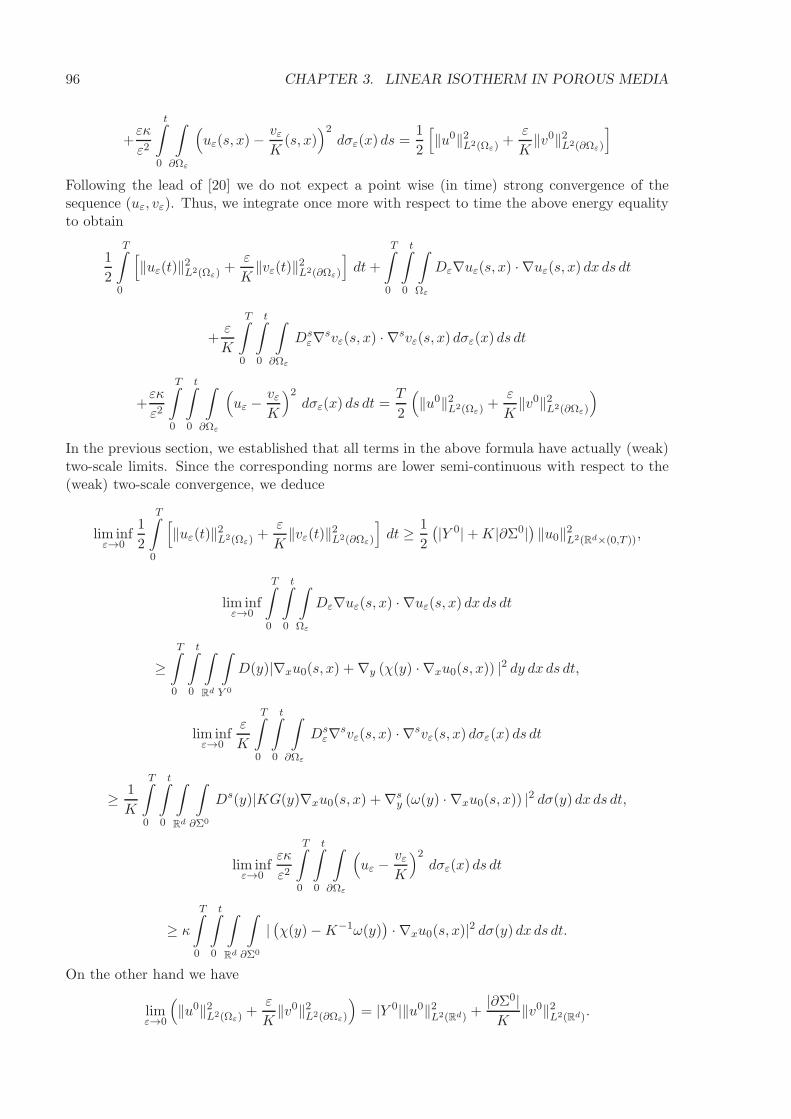
96 CHAPTER 3. LINEAR ISOTHERM IN POROUS MEDIA
+εκ
ε2
t∫
0
∫
∂Ωε
(uε(s, x)−
vεK
(s, x))2
dσε(x) ds =1
2
[‖u0‖2L2(Ωε)
+ε
K‖v0‖2L2(∂Ωε)
]
Following the lead of [20] we do not expect a point wise (in time) strong convergence of thesequence (uε, vε). Thus, we integrate once more with respect to time the above energy equalityto obtain
1
2
T∫
0
[‖uε(t)‖2L2(Ωε)
+ε
K‖vε(t)‖2L2(∂Ωε)
]dt+
T∫
0
t∫
0
∫
Ωε
Dε∇uε(s, x) · ∇uε(s, x) dx ds dt
+ε
K
T∫
0
t∫
0
∫
∂Ωε
Dsε∇svε(s, x) · ∇svε(s, x) dσε(x) ds dt
+εκ
ε2
T∫
0
t∫
0
∫
∂Ωε
(uε −
vεK
)2dσε(x) ds dt =
T
2
(‖u0‖2L2(Ωε)
+ε
K‖v0‖2L2(∂Ωε)
)
In the previous section, we established that all terms in the above formula have actually (weak)two-scale limits. Since the corresponding norms are lower semi-continuous with respect to the(weak) two-scale convergence, we deduce
lim infε→0
1
2
T∫
0
[‖uε(t)‖2L2(Ωε)
+ε
K‖vε(t)‖2L2(∂Ωε)
]dt ≥ 1
2
(|Y 0|+K|∂Σ0|
)‖u0‖2L2(Rd×(0,T )),
lim infε→0
T∫
0
t∫
0
∫
Ωε
Dε∇uε(s, x) · ∇uε(s, x) dx ds dt
≥T∫
0
t∫
0
∫
Rd
∫
Y 0
D(y)|∇xu0(s, x) +∇y (χ(y) · ∇xu0(s, x)) |2 dy dx ds dt,
lim infε→0
ε
K
T∫
0
t∫
0
∫
∂Ωε
Dsε∇svε(s, x) · ∇svε(s, x) dσε(x) ds dt
≥ 1
K
T∫
0
t∫
0
∫
Rd
∫
∂Σ0
Ds(y)|KG(y)∇xu0(s, x) +∇sy (ω(y) · ∇xu0(s, x)) |2 dσ(y) dx ds dt,
lim infε→0
εκ
ε2
T∫
0
t∫
0
∫
∂Ωε
(uε −
vεK
)2dσε(x) ds dt
≥ κ
T∫
0
t∫
0
∫
Rd
∫
∂Σ0
|(χ(y)−K−1ω(y)
)· ∇xu0(s, x)|2 dσ(y) dx ds dt.
On the other hand we have
limε→0
(‖u0‖2L2(Ωε)
+ε
K‖v0‖2L2(∂Ωε)
)= |Y 0|‖u0‖2L2(Rd) +
|∂Σ0|K
‖v0‖2L2(Rd).

3.10. STRONG CONVERGENCE 97
Summing up those limits and recognizing the formula for D yields the inequality
1
2
(|Y 0|+K|∂Σ0|
)‖u0‖2L2(Rd×(0,T )) +
T∫
0
t∫
0
∫
Rd
D∇xu0(s, x) · ∇xu0(s, x) dx ds dt
≤ T
2
(|Y 0|‖u0‖2L2(Rd) +
|∂Σ0|K
‖v0‖2L2(Rd)
). (3.46)
However, if we write the same type of time integral of the energy equality for the homogenizedequation (3.28), we get an equality with the same left hand side but a different right hand side
1
2
[|Y 0|+K|∂Σ0|
]‖u0‖2L2(Rd×(0,T )) +
T∫
0
t∫
0
∫
Rd
D∇u0(s, x) · ∇u0(s, x) dx ds dt
=T
2(|Y 0|+K|∂Σ0|)‖|Y0|u0 + |∂Σ0|v0‖2L2(Rd). (3.47)
It is easy to check that the two right hand sides in (3.46) and (3.47) coincide if and only if
‖u0 −K−1v0‖2L2(Rd) = 0,
which is precisely our assumption of well prepared initial data. Therefore, under this assumptionwe deduce that (3.46) is not an inequality but rather an equality, which in turn implies that allthe previous lower semi-continuity of norm sequences are actually exact convergence. We canthus apply Proposition 2.6.7 and conclude to the strong convergence (see Section 2.6 of Chapter2 for details if necessary).We now turn to the case of general initial data (u0, v0) ∈ L2(Rd) × H1(Rd). Let us considera small δ0 > 0, to be chosen precisely at the end of the proof. Due to Lemma 3.6.1 on apriori estimates, by a contradiction argument, it follows that there exists a time sequence δε,δ0/2 ≤ δε ≤ δ0, converging to some limit δ, δ0/2 ≤ δ ≤ δ0, and a positive constant C, whichdoes not depend on δ0 or on ε (but only on the initial data), such that
‖uε(., δε)‖2H1(Ωε)≤ C/δ0, ε‖vε(., δε)‖2H1(∂Ωε)
≤ C/δ0,
ε‖Kuε(., δε)− vε(., δε)‖2L2(∂Ωε)≤ Cε2/δ0.
(3.48)
We now follow an idea of [20] which amounts to consider system (3.11)-(3.13) on a smaller timeinterval (δε, T ) where δε ≥ δ0/2 > 0 is such that the initial data at this time should be almostwell-prepared because of parabolic dissipation on the earlier time interval (0, δε). We decomposethe solution (uε, vε) of (3.11)-(3.13) as
uε(t, x) = u1,ε(t, x) + u2,ε(t, x) and vε(t, x) = v1,ε(t, x) + v2,ε(t, x),
in such way that the initial data are well prepared for the first problem while the solution of thesecond one will converge strongly to zero
∂u1,ε∂t
+1
εbε · ∇u1,ε − div (Dε∇u1,ε) = 0 in (δε, T )× Ωε,
−Dε
ε∇u1,ε · n =
∂v1,ε∂t
+1
εbsε · ∇sv1,ε − divs (Ds
ε∇sv1,ε) on (δε, T )× ∂Ωε,
−Dε
ε∇u1,ε · n =
κ
ε2
(u1,ε −K−1v1,ε
)on (δε, T )× ∂Ωε,
u1,ε(δε, x) = uε(δε, x), v1,ε(δε, x) = Kuε(δε, x),
(3.49)

98 CHAPTER 3. LINEAR ISOTHERM IN POROUS MEDIA
and
∂u2,ε∂t
+1
εbε · ∇u2,ε − div (Dε∇u2,ε) = 0 in (δε, T )× Ωε,
−Dε
ε∇u2,ε · n =
∂v2,ε∂t
+1
εbsε · ∇sv2,ε − divs (Ds
ε∇sv2,ε) on (δε, T )× ∂Ωε,
−Dε
ε∇u2,ε · n =
κ
ε2
(u2,ε −K−1v2,ε
)on (δε, T )× ∂Ωε,
u2,ε(δε, x) = 0, v2,ε(δε, x) = vε(δε, x)−Kuε(δε, x).
(3.50)
Since (3.50) is similar in structure to (3.11)-(3.13), the standard a priori estimate of Lemma3.6.1, together with estimate (3.48) for the initial data at time δε, yields for any t ≥ δε
‖u2,ε(., t)‖2L2(Ωε)+ ε‖v2,ε(., t)‖2L2(∂Ωε)
≤ Cε2/δ0.
Thus, the sequence (u2,ε, v2,ε) strongly converges to 0. The initial data in (3.49) are well preparedbut we cannot apply directly our previous results because the initial time δε 6= 0 is varying withε. The new difficulty is to prove that the initial data of (3.49) strongly two-scale converge withdrift to some limit.Let us recall the existence of a uniformly bounded extension operator [1] from H1(Ωε) intoH1(Rd). Thus, the sequence uε(δε, x) can be thought of being defined in the whole space Rd
and, by virtue of (3.48) it satisfies the bound ‖uε(δε, x)‖2H1(Rd)≤ C/δ0. Shifting the sequence
does not change its bound, so we have
‖uε(δε, x+ (b∗/ε)δε)‖2H1(Rd) ≤ C/δ0. (3.51)
Together with Lemma 3.10.2 which says that the L2-norm of uε(δε, x+(b∗/ε)δε) does not escapeat infinity, we deduce from (3.51) that this sequence is (pre-)compact in L2(Rd). Therefore, upto a subsequence, uε(δε, x+ (b∗/ε)δε) converges strongly to some limit u0(x) in L2(Rd).Thus we can use the same arguments as in the case of well-prepared initial data to conclude thatu1,ε and v1,ε strongly two-scale converge with drift to u(t, x) and Ku(t, x) respectively where usatisfies the following limit equation of (3.49)
Kd ∂tu = divx (D∇xu) in (δ, T )× Rd
Kd u(δ, x) = |Y 0|u0(x) + |∂Σ0|d−1u0(x), x ∈ Rd
(3.52)
where Kd = |Y 0|+K|∂Σ0|d−1 and D is given by (3.29). In particular,
limε→0
‖u1,ε‖2L2((δε,T )×Ωε)= |Y 0|‖u‖2
L2((δ,T )×Rd)
andlimε→0
ε‖v1,ε‖2L2((δε,T )×∂Ωε)= K2|∂Σ0|‖u‖2
L2((δ,T )×Rd).
Of course, since uε was converging weakly to u0, we deduce that u(t, x) = u0(t, x) for t ≥ δ, and
limε→0
‖uε‖2L2((δε,T )×Ωε)= |Y 0|‖u0‖2L2((δ,T )×Rd)
limε→0
ε‖vε‖2L2((δε,T )×∂Ωε)= K2|∂Σ0|‖u0‖2L2((δ,T )×Rd)
.(3.53)
Now, let us assume that there is a lack of strong two-scale convergence for (uε, vε), namely thatthe L2-norm of this sequence is not continuous (as required by (??) in Proposition 2.6.7). Inother words, either
limε→0
‖uε‖2L2((0,T )×Ωε)> |Y 0|‖u0‖2L2(Rd×(0,T )) (3.54)

3.10. STRONG CONVERGENCE 99
orlimε→0
ε‖vε‖2L2((0,T )×∂Ωε)> K2|∂Σ0|‖u0‖2L2(Rd×(0,T )). (3.55)
Lemma 3.6.1 implies that ‖uε(t)‖2L2(Ωε)+ ε‖vε(t)‖2L2(∂Ωε)
≤ C uniformly in time. So, we canfind a small δ0 > 0 such that, the same strict inequalities hold true on a smaller time interval,namely, either
lim infε→0
‖uε‖2L2((δ,T )×Ωε)> |Y 0|‖u0‖2L2((0,T )×Rd) for any 0 < δ < δ0, (3.56)
orlim infε→0
ε‖vε‖2L2((δ,T )×∂Ωε)> K2|∂Σ0|‖u0‖2L2((0,T )×Rd) for any 0 < δ < δ0. (3.57)
Obviously, (3.56) or (3.57) contradicts (3.53). Therefore, there must be continuity of the L2-norm of (uε, vε) and both (3.54) and (3.55) must be equalities. Thus, we have proved the strongtwo-scale convergence with drift in case of a general initial data.
Lemma 3.10.2. Let uε(t, x) be the solution of (3.11)-(3.13). For any δ > 0 there is R(δ) > 0such that, for any t ∈ [0, T ],
∥∥∥uε(t, x+
b∗
εt)∥∥∥
L2(Ωε∩x≥R(δ))≤ δ.
Proof. We again follow an idea of [20]. Let φ ∈ C∞(R) be a cut–off function such that 0 ≤φ(r) ≤ 1, φ = 0 for r ≤ 1, φ = 1 for r ≥ 2. For x ∈ Rd, denote φR(x) = φ(|x|/R) andφεR(t, x) = φR(x − b∗t/ε). In the variational formulation (3.40) of system (3.11)-(3.12) wetake the test function uε(t, x)φεR(t, x), vε(t, x)φεR(t, x) and we integrate by parts the time andconvective derivatives (calculations are shown one term at a time)
2
t∫
0
∫
Ωε
∂uε∂t
(s, x)uε(s, x)φεR(s, x) ds dx =
t∫
0
∫
Ωε
b∗
ε· ∇φεR(s, x)(uε(s, x))2 ds dx
+
∫
Ωε
φεR(t, x)(uε(t, x))2 dx−
∫
Ωε
φR(x)(u0(x))2 dx,
2
t∫
0
∫
Ωε
bεε· ∇uε(s, x)uε(s, x)φεR(s, x) ds dx = −
t∫
0
∫
Ωε
bεε· ∇φεR(s, x)(uε(s, x))2 ds dx,
2ε
K
t∫
0
∫
∂Ωε
∂vε∂t
φεRvε ds dσ(x) =
t∫
0
∫
∂Ωε
b∗
K· ∇φεR(vε)2 ds dσ(x)
+ε
K
∫
∂Ωε
φεR(vε)2 dσ(x)− ε
K
∫
∂Ωε
φR(x)(v0(x))2 dσ(x),
2
K
t∫
0
∫
∂Ωε
bsε · ∇svεvεφεR ds dσ(x) = − 1
K
t∫
0
∫
∂Ωε
(vε)2bsε · ∇sφεR ds dσ(x).
This yields
1
2
∫
Ωε
φεR(t, x)(uε(t, x))2 dx+
t∫
0
∫
Ωε
Dε∇uε · ∇uεφεR ds dx

100 CHAPTER 3. LINEAR ISOTHERM IN POROUS MEDIA
+ε
2K
∫
∂Ωε
φεR(t, x)(vε(t, x))2 dσ(x) +
ε
K
t∫
0
∫
∂Ωε
Dsε∇svε · ∇svεφ
εR ds dσ(x)
+κε
ε2
t∫
0
∫
∂Ωε
φεR(uε −K−1vε
)2ds dσ(x)
= −t∫
0
∫
Ωε
uεDε∇uε · ∇φεR ds dx− ε
K
t∫
0
∫
∂Ωε
vεDsε∇svε · ∇sφεR ds dσ(x)
+
t∫
0
∫
Ωε
1
ε(bε − b∗) · ∇φεR (uε)
2ds dx+1
2
∫
Ωε
φR(x)(u0(x))2 dx
+
t∫
0
∫
∂Ωε
1
K(bsε − b∗) · ∇sφεR(vε)
2ds dσ(x) +ε
2K
∫
∂Ωε
φR(x)(v0(x))2 dσ(x) (3.58)
Due to the a priori estimate of Lemma 3.6.1 and the definition of φR, the first and secondintegrals on the right hand side of (3.58) are uniformly bounded by C/R. The terms involvingthe initial data (u0(x), v0(x)) do not depend on ε and tend to zero as R tends to ∞. To get abound on the remaining (convective) terms on the right hand side of (3.58), we rely again on theauxiliary problem (3.42) which allows us to remove the ε−1 singularity of the convective terms
t∫
0
∫
Ωε
1
ε(bε − b∗) · ∇φεR(uε)2ds dx+
t∫
0
∫
∂Ωε
1
K(bsε − b∗) · ∇sφεR(vε)
2ds dσ(x) (3.59)
= εd∑
i=1
t∫
0
∫
Ωε
∇αεi · ∇
((uε)
2∂xiφεR
)ds dx+K
t∫
0
∫
∂Ωε
∇φεR ·(b∗ − bsε
) ((uε)
2 −K−2(vε)2)ds dσ(x).
Since (u2ε − K−2v2ε) = (uε + K−1vε)(uε − K−1vε) and ε∇αεi (x) = (∇yαi) (x/ε), the a priori
estimates of Lemma 3.6.1 imply that (3.59) is uniformly bounded by C/R too, which yields thedesired statement.
3.11 Slow reaction
We shall consider a different scaling for the reaction as is done in [81], [109]. It should be noted,however, that the scaling considered in [81] and [109] isn’t in the strong convection regime. Weshall only be scaling the reaction parameter by κ → ε2κ in (3.11)-(3.13). In other words, thereaction is considered to be small. As far as this section is considered, we shall be working withthe following coupled parabolic equations in the ε-periodic porous domain.
∂uε∂t
+1
εbε · ∇uε − div (Dε∇uε) = 0 in (0, T ) × Ωε, (3.60)
−Dε
ε∇uε · n =
∂vε∂t
+1
εbsε · ∇svε − divs (Ds
ε∇svε) = κ(uε −
vεK
)on (0, T )× ∂Ωε, (3.61)
uε(0, x) = uin(x) in Ωε, vε(0, x) = vin(x) on ∂Ωε. (3.62)
Under this scaling, the homogenization result is very different from the one obtained in theprevious sections.

3.11. SLOW REACTION 101
Lemma 3.11.1. There exists a constant C, independent of ε, such that
‖uε‖L∞((0,T );L2(Ωε)) +√ε‖vε‖L∞((0,T );L2(∂Ωε))
+‖∇uε‖L2((0,T )×Ωε) +√ε‖∇svε‖L2((0,T )×∂Ωε)
+√ε∥∥∥uε −
vεK
∥∥∥L∞((0,T );L2(∂Ωε))
≤ C(∥∥uin
∥∥L2(Rd)
+ ‖vin‖H1(Rd)
),
(3.63)
Proof. As usual, the approach we shall take to derive the a priori estimates is via energy esti-mates. Let us multiply (3.60) by uε and integrate over Ωε
1
2
d
dt
∫
Ωε
|uε|2 dx+
∫
Ωε
Dε∇uε · ∇uε dx+ κε
∫
∂Ωε
(uε − vε) uε dσ(x) = 0.
Then, let us multiply the second part of (3.61) by εvε and integrate over ∂Ωε
ε
2
d
dt
∫
∂Ωε
|vε|2 dσ(x) + ε
∫
∂Ωε
Dsε∇svε · ∇svε dσ(x)− κε
∫
∂Ωε
(uε − vε) vε dσ(x) = 0.
Adding the above two equations results in the energy equality
1
2
d
dt
∫
Ωε
|uε|2 dx+
∫
Ωε
Dε∇uε · ∇uε dx+ε
2
d
dt
∫
∂Ωε
|vε|2 dσ(x)
+ε
∫
∂Ωε
Dsε∇svε · ∇svε dσ(x) + κε
∫
∂Ωε
(uε − vε)2 dσ(x) = 0
Integrating the above energy equality with respect to time on the time interval (0, T ) yields thea priori estimates as in (3.63).
In the homogenization result regarding (3.11)-(3.13) given by the Proposition 3.7.2, the induceddrift b∗ in the concentration profiles was given by (3.27). Both the bulk velocity field b and thesurface velocity field bs contributed to the drift b∗ as suggested by the expression (3.27). Also,the drift velocity happened to be the same for both the bulk and surface concentrations. Thetwo-scale limits for both uε and vε were given by u0 which is characterized by the singleeffective diffusion equation (3.28). Here the situations is different. We consider different driftvelocities for the two concentrations.
uε(t, x) =
∞∑
i=0
εiui
(t, x− b∗1t
ε,x
ε
)(3.64)
and
vε(t, x) =
∞∑
i=0
εivi
(t, x− b∗2t
ε,x
ε
)(3.65)
Proposition 3.11.2. Define two constants b∗1, b∗2 ∈ Rd by
b∗1 =1
|Y 0|
∫
Y 0
b(y) dy and b∗2 =1
|∂Σ0|
∫
∂Σ0
bs(y) dσ(y). (3.66)
Then the solution (uε, vε) for (3.60)-(3.62), under the assumption (3.64)-(3.65), formally satisfy
uε(t, x) ≈ u0
(t, x− b∗1t
ε
)+ εu1
(t, x− b∗1t
ε,x
ε
)

102 CHAPTER 3. LINEAR ISOTHERM IN POROUS MEDIA
vε(t, x) ≈ v0
(t, x− b∗2t
ε
)+ εv1
(t, x− b∗2t
ε,x
ε
).
In case the drift velocities b∗1 = b∗2 = b∗ (say), the zero order approximations u0, v0 satisfy thefollowing coupled effective equations
|Y 0|∂u0∂t
+ κ|∂Σ0|(u0 −
v0K
)= div(A∗∇xu0) in Rd × (0, T ),
|∂Σ0|∂v0∂t
− κ|∂Σ0|(u0 −
v0K
)= div(B∗∇xv0) in Rd × (0, T )
(3.67)
with the dispersion tensors A∗ and B∗ given by
A∗ij =
∫
Y 0
D(y) (∇yχi + ei) · (∇yχj + ej) dy (3.68)
B∗ij =
∫
∂Σ0
Ds(y)(∇s
yωi + ei)·(∇s
yωj + ej)dσ(y) (3.69)
with (χ, ω) = (χi, ωi)1≤i≤d being the solution of the cell problem such that
u1(t, x, y) =
d∑
i=1
χi(y)∂u0∂xi
(t, x) v1(t, x, y) =
d∑
i=1
ωi(y)∂v0∂xi
(t, x). (3.70)
and the cell problem satisfied by (χi, ωi), for every 1 ≤ i ≤ d, is
b(y) · ∇yχi − divy(D(∇yχi + ei)) = (b∗ − b) · ei in Y 0,
−D(∇yχi + ei) · n = 0 on ∂Σ0,
y → χi(y) Y − periodic.
(3.71)
and the surface cell problem satisfied by ωi isbs(y) · ∇s
yωi − divsy(Ds(∇s
yωi +Kei)) = (b∗ − bs) · ei on ∂Σ0,
y → ωi(y) Y − periodic.(3.72)
In case the drift velocities b∗1 6= b∗2, the zero order approximations u0 and v0 satisfy the followinghomogenized equations.
|Y 0|∂u0
∂t+ κ|∂Σ0|u0 = div(A∗∇xu0) in Rd × (0, T ) (3.73)
|∂Σ0|∂v0
∂t+κ
K|∂Σ0|v0 = div(B∗∇xv0) in Rd × (0, T ) (3.74)
The dispersion tensors A∗ and B∗ are given by (3.68) and (3.69) respectively which are in termsof the solutions (χi, ωi) for the cell problems
b(y) · ∇yχi − divy(D(∇yχi + ei)) = (b∗1 − b) · ei in Y 0,
−D(∇yχi + ei) · n = 0 on ∂Σ0,
y → χi(y) Y -periodic.
(3.75)
bs(y) · ∇s
yωi − divsy(Ds(∇s
yωi +Kei)) = (b∗2 − bs) · ei on ∂Σ0,
y → ωi(y) Y -periodic.(3.76)

3.11. SLOW REACTION 103
Proof. Case I: b∗1 = b∗2 = b∗
Plugging the expressions for uε and vε from (3.64)-(3.65) into the coupled equations (3.60)-(3.62),we identify the cascade of equations as the coefficients of various powers of ε.
At order ε−2:
b(y) · ∇yu0 − divy(D(y)∇yu0) = 0 in Y 0,
−D∇yu0 · n = 0 on ∂Σ0,
bs(y) · ∇syv0 − divsy(D
s(y)∇syv0) = 0 on ∂Σ0,
y → (u0(y), v0(y)) Y − periodic.
(3.77)
From (3.78), it follows that (u0, v0) are independent of the fast variable y. Note that there is nocontribution from the reaction in (3.77) because of the chosen scaling for the reaction rate.At order ε−1:
−b∗ · ∇xu0 + b(y) · (∇xu0 +∇yu1)− divy(D(y)(∇xu0 +∇yu1)) = 0 in Y 0,
−D(y)(∇xu0 +∇yu1) · n = 0 on ∂Σ0,
−b∗ · ∇xv0 + bs(y) · (∇xv0 +∇syv1)− divsy(D
s(y)(∇xv0 +∇syv1)) = 0 on ∂Σ0,
y → (u1(y), v1(y)) Y − periodic.
(3.78)
By linearity of (3.78) we deduce that
u1(t, x, y) = χ(y) · ∇xu0 and v1(t, x, y) = ω(y) · ∇xv0
where χi and ωi are the solutions of the cell problems (3.71) and (3.72) respectively. Thecompatibility condition for the well-posedness of the cell problems give the expressions for thecommon drift velocity b∗ given by (3.66).
At order ε0:
∂u0∂t
− b∗ · ∇xu1 + b(y) · (∇xu1 +∇yu2)
−divx(D(y)(∇xu0 +∇yu1))− divy(D(y)(∇xu1 +∇yu2)) = 0 in Y 0,
−D(y)(∇yu2 +∇xu1) · n = κ(u0 −
v0K
)on ∂Σ0,
∂v0∂t
− b∗ · ∇xv1 + bs(y) · (∇xu1 +∇syu2)− divx(D
s(y)(∇xv0 +∇syv1))
−divsy(Ds(y)(∇xv1 +∇s
yv2)) = κ(u0 −
v0K
)on ∂Σ0,
y → (u2(y), v2(y)) Y − periodic.
(3.79)
The compatibility conditions for the well-posedness of (3.79) for (u2, v2) results in the coupledhomogenized equation (3.67).
Case II: b∗1 6= b∗2
Now let us analyse the case where the bulk drift and the surface drift don’t match. Uponplugging in (3.64)-(3.65) into the coupled equations (3.60)-(3.62), we find the same system as(3.77) at order ε−2. Also at order ε−1, we find a system similar to (3.78) except for the differentdrifts in the bulk and on the surface of the pore. The system we get is the following.

104 CHAPTER 3. LINEAR ISOTHERM IN POROUS MEDIA
−b∗1 · ∇xu0 + b(y) · (∇xu0 +∇yu1)− divy(D(y)(∇xu0 +∇yu1)) = 0 in Y 0,
−D(y)(∇xu0 +∇yu1) · n = 0 on ∂Σ0,
−b∗2 · ∇xv0 + bs(y) · (∇xv0 +∇syv1)− divsy(D
s(y)(∇xv0 +∇syv1)) = 0 on ∂Σ0,
y → (u1(y), v1(y)) Y -periodic.
(3.80)
The values of b∗1 and b∗2 from (3.66) guarantee the well-posedness of the above system. Byinvoking linearity of (3.80), we deduce that the first order correctors u1 and v1 can be decomposedin terms of the cell solutions and the gradient of the zero order approximation as in (3.70). Thecell problems corresponding to this case of different bulk and surface drift velocities are (3.75)and (3.75).Next, at the order ε0 we recognize the following equations for u2 and v2.
∂u0∂t
− b∗ · ∇xu1 + b(y) · (∇xu1 +∇yu2)
−divx(D(y)(∇xu0 +∇yu1))− divy(D(y)(∇xu1 +∇yu2)) = 0 in Y 0,
−D(y)(∇yu2 +∇xu1) · n = κu0 on ∂Σ0,
y → u2(y) Y -periodic.
(3.81)
∂v0∂t
− b∗ · ∇xv1 + bs(y) · (∇xu1 +∇syu2)− divx(D
s(y)(∇xv0 +∇syv1))
−divsy(Ds(y)(∇xv1 +∇s
yv2)) = − κ
Kv0 on ∂Σ0,
y → v2(y) Y -periodic.
(3.82)
Notice that the coupling terms haven’t appeared in the above two equations (3.81) and (3.82).The compatibility condition for the well-posedness of (3.81) for u2 results in the homogenizedequation (3.73) and the compatibility condition for the well-posedness of (3.82) for v2 results inthe homogenized equation (3.73).
Now, we state a result that justifies the upscaling done formally in Proposition 3.11.2.
Proposition 3.11.3. Assume that
b∗1 =1
|Y 0|
∫
Y 0
b(y) dy =1
|∂Σ0|
∫
∂Σ0
bs(y) dσ(y) = b∗2 = b∗(say).
There exists u0, v0 ∈ L2((0, T );H1(Rd)), u1 ∈ L2((0, T ) × Rd;H1#(Y
0)) and v1 ∈ L2((0, T ) ×Rd;H1
#(∂Σ0)) such that the solution sequences uε and vε, two-scale converge with drift b∗,
in the following sense.
uε2−drift−−−− u0(t, x)
vε2s−drift−−−−− v0(t, x)
∇uε 2−drift−−−− ∇xu0(t, x) +∇yu1(t, x, y)
∇svε2s−drift−−−−− ∇xv0(t, x) +∇s
yv1(t, x, y)(uε −
vεK
)2s−drift−−−−− u0(t, x)−
v0K
(t, x)
(3.83)

3.11. SLOW REACTION 105
The two-scale limits u0 and v0 satisfy the following coupled effective equations.
|Y 0|∂u0∂t
+ κ|∂Σ0|(u0 −
v0K
)= div(A∗∇xu0) in Rd × (0, T ),
|∂Σ0|∂v0∂t
− κ|∂Σ0|(u0 −
v0K
)= div(B∗∇xv0) in Rd × (0, T )
(3.84)
The dispersion tensors A∗ and B∗ are given by (3.68) and (3.69) respectively which are in termsof the solutions (χi, ωi) for the cell problem
b(y) · ∇yχi − divy(D(∇yχi + ei)) = (b∗ − b) · ei in Y 0,
−D(∇yχi + ei) · n = 0 on ∂Σ0,
bs(y) · ∇syωi − divsy(D
s(∇syωi +Kei)) = (b∗ − bs) · ei on ∂Σ0,
y → (χi(y), ωi(y)) Y − periodic.
(3.85)
In case the drift velocities b∗1 6= b∗2, the two-scale limits as given in (3.83) hold except for the lastline. The homogenized equations satisfied by u0 and v0 are decoupled.
|Y 0|∂u0
∂t+ κ|∂Σ0|u0 = div(A∗∇xu0) in Rd × (0, T ) (3.86)
|∂Σ0|∂v0
∂t+κ
K|∂Σ0|v0 = div(B∗∇xv0) in Rd × (0, T ) (3.87)
The dispersion tensors A∗ and B∗ are given by (3.68) and (3.69) respectively which are in termsof the solutions (χi, ωi) for the cell problems
b(y) · ∇yχi − divy(D(∇yχi + ei)) = (b∗1 − b) · ei in Y 0,
−D(∇yχi + ei) · n = 0 on ∂Σ0,
y → χi(y) Y − periodic.
(3.88)
bs(y) · ∇s
yωi − divsy(Ds(∇s
yωi +Kei)) = (b∗2 − bs) · ei on ∂Σ0,
y → ωi(y) Y − periodic.(3.89)
Proof. Suppose b∗1 = b∗2 = b∗ ∈ Rd. The compactness of the sequences in (3.83) follow di-rectly from the a priori estimates (3.63) and the compactness results of Propositions 2.3.3, 2.7.3from Chapter 2. let us consider the variational formulation for (3.60)-(3.62) by test functions(φε, εK
−1ψε):
φε(t, x) = φ(t, x− b∗t
ε
)+ ε φ1
(t, x− b∗t
ε,x
ε
)
and
ψε(t, x) = ψ(t, x− b∗t
ε
)+ εψ1
(t, x− b∗t
ε,x
ε
).
T∫
0
∫
Ωε
[∂uε∂t
φε +1
εbε · ∇uεφε +Dε∇uε · ∇φε
]dx dt
+ε
K
T∫
0
∫
∂Ωε
[∂vε∂t
ψε +1
εbsε · ∇svεψε +Ds
ε∇svε · ∇sψε
]dσε(x) dt

106 CHAPTER 3. LINEAR ISOTHERM IN POROUS MEDIA
+εκ
T∫
0
∫
∂Ωε
(uε −
vεK
)(φε −
ψε
K
)dσε(x) dt = 0.
We shall use the auxiliary problem (3.42) to take care of the singular terms in the above vari-ational formulation as is done in Section 3.9. Taking (φ,ψ) ≡ 0, we shall pass to the limit inthe above variational formulation taking into account (3.83) resulting in the cell problem (3.85).Then we take (φ1, ψ1) ≡ 0 in the variational formulation followed by passing to limit in arrivingat a variational formulation for the coupled effective equations (3.84).
Now for the case b∗1 6= b∗2. Taking the test functions with different drifts as
φε(t, x) = φ(t, x− b∗1t
ε
)+ ε φ1
(t, x− b∗1t
ε,x
ε
)
and
ψε(t, x) = ψ(t, x− b∗2t
ε
)+ εψ1
(t, x− b∗2t
ε,x
ε
).
The calculations carry on as before except for the coupled term
κε
T∫
0
∫
∂Ωε
(uε −
vεK
)(φ(t, x− b∗1t
ε
)− ψ
K
(t, x− b∗2t
ε
))dσε(x) dt
2s−drift−−−−− κ
T∫
0
∫
Rd
∫
∂Σ0
u0(t, x)φ(t, x) dσ(y) dx dt +κ
K2
T∫
0
∫
Rd
∫
∂Σ0
v0(t, x)ψ(t, x) dσ(y) dx dt
as the two-scale limit for uε vanishes for the test functions with drift b∗2 and the two-scale limitfor vε vanishes for the test functions with the drift b∗1. Taking into consideration the abovetwo-scale limit and redoing the calculations as in the proof of the homogenization process ofSection 3.9, we arrive at the homogenized equations (3.86) and (3.87) for u0 and v0 respectively.Also, the cell problem isn’t coupled anymore.
3.12 Compressible flows
Until now, we have had the assumption of null divergence on the velocity fields b and bs. Inthis section, we shall be ignoring this assumption. We shall, however, leave the assumption ofperiodicity. We present the analysis for a convection-diffusion equation of a single solute in theabsence of reactions. The model we wish to analyze is the following.
∂uε∂t
+1
εbε · ∇uε − div (Dε∇uε) = 0 in (0, T ) × Ωε, (3.90)
−Dε∇uε · n = 0 on (0, T ) × ∂Ωε, (3.91)
uε(0, x) = uin(x) in Ωε (3.92)
We make the regularity assumption b ∈ L∞# (Ωf ;R
d) on the velocity field. Also, we assume thatdiv(b) ∈ L∞
# (Ωf ;R) although this regularity can be slightly weakened. We also assume thatb(y) · n ∈ L∞
# (∂Ωs;R). Let us derive energy estimates for our model. Multiplying (3.90) by thesolution uε
1
2
d
dt
∫
Ωε
|uε|2 dx+1
2ε
∫
Ωε
bε · ∇|uε|2 dx+
∫
Ωε
Dε∇uε · ∇uε dx = 0

3.12. COMPRESSIBLE FLOWS 107
After an integration by parts
1
2
d
dt
∫
Ωε
|uε|2 dx− 1
2ε
∫
Ωε
div(bε)|uε|2 dx− 1
2ε
∫
∂Ωε
bε · n|uε|2 dσ(x) +∫
Ωε
Dε∇uε · ∇uε dx = 0
which implies
1
2
d
dt‖uε‖2L2 +
∫
Ωε
Dε∇uε · ∇uε dx =1
2ε
∫
Ωε
div(bε)|uε|2 dx+1
2ε
∫
∂Ωε
bε · n|uε|2 dσ(x) (3.93)
We have the following Poincare type inequality (proved in [67])
ε
∫
∂Ωε
|uε|2 dσ(x) ≤ δε
∫
Ωε
|∇uε|2 dx+1
δε
∫
Ωε
|uε|2 dx (3.94)
for some positive constant depending on ε. Using (3.94), we can bound the right hand side of(3.93) by
≤ 1
2ε
∥∥∥div(bε)∥∥∥L∞
∥∥∥uε∥∥∥2
L2+
1
δε
∥∥∥bε∥∥∥L∞
∥∥∥uε∥∥∥2
L2+ δε
∥∥∥∇uε∥∥∥2
L2
=⇒ 1
2
d
dt‖uε‖2L2 ≤ 1
2ε
(‖div(bε)‖L∞ +
1
δε‖bε‖L∞
)‖uε‖2L2
Thus by Gronwall’s inequality
‖uε‖2 ≤ ‖uin‖2 exp( t∫
0
(1ε‖div(bε)‖L∞ +
1
δε‖bε‖L∞
)ds)
=⇒ ‖uε‖2 ≤ exp( tε‖div(bε)‖L∞ +
t‖bε‖L∞
εδε
)‖uin‖2
So, it is not possible to derive a priori estimates for uε with constant independent of ε. However,for a fixed ε, we have the following estimates.
‖uε‖L2((0,T );H1(Ωε)) ≤ Cε (3.95)
To upscale the model at hand, we tend to employ the method of two-scale convergence. AsPropositions 2.6.4 and 2.6.6 suggest, we need uniform estimates independent of ε. But theconstant Cε in (3.95) isn’t independent of ε. So we cannot straightaway apply the compactnessresults of Chapter 2. Here we shall take cues from [25] where a method of Factorization isemployed in arriving at a homogenized equation for a convection-diffusion-reaction equationwith a divergent velocity flow.The principle of the Factorization method is quite simple as explained in Section 2.8 of Chapter2. In the formal analysis of Section 3.7, we deduced that the first term in the ansatz for thesolute concentration uε is independent of the fast variable y. In case of some partial differentialequations, however, the oscillations are present even in the first term of the ansatz. Thereare examples where one can factor out the oscillations from the solutions. This method wasintroduced in [161]. The oscillations that we factor out comes off as a eigenfunction for aspectral problem.
b(y) · ∇yϕ− divy
(D(y)∇yϕ
)= λϕ in Y 0,
−D(y)∇yϕ · n = 0 on ∂Σ0,
y → ϕ(y) Y -periodic.
(3.96)

108 CHAPTER 3. LINEAR ISOTHERM IN POROUS MEDIA
The adjoint of the above spectral problem.
−divy(b(y)ϕ∗)− divy
(D(y)∇yϕ
∗)= λϕ∗ in Y 0,
D(y)∇yϕ∗ · n+ b(y) · nϕ∗ = 0 on ∂Σ0,
y → ϕ∗(y) Y -periodic.
(3.97)
The existence of the first simple eigenvalue λ > 0 and the first eigenfunctions ϕ > 0 and ϕ∗ > 0for the spectral and the adjoint spectral problem (3.96)-(3.97) follows from the Krein-RutmanTheorem [108], [152]. The uniqueness follows from the chosen normalization.
∫
Y 0
ϕ(y)ϕ∗(y) dy = 1. (3.98)
Using the eigenfunction associated with both the direct and the adjoint spectral cell problems(3.96) and (3.97), we define modified velocity field and diffusion matrix as
b(y) = ϕϕ∗b(y) + ϕD(y)∇yϕ∗ − ϕ∗D(y)∇yϕ (3.99)
andD(y) = ϕϕ∗D(y) (3.100)
We consider the following ansatz for uε
uε(t, x) = exp(−λt/ε2)∑
i≥0
εiui
(t, x− b∗t
ε,x
ε
). (3.101)
Proposition 3.12.1. If the ansatz for the solution uε of (3.90)-(3.92) in (3.101) is true, thenthe solution formally satisfies
uε(t, x) ≈ exp(−λt/ε2)ϕ(xε
)[v(t, x− b∗
εt)+ ε
d∑
i=1
∂v
∂xi
(t, x− b∗
εt)ωi
(xε
)](3.102)
where ωi(y), for every 1 ≤ i ≤ d, satisfy a so called cell problem.
b(y) ·(∇yωi + ei
)− divy
(D(y)
(∇yωi + ei
))= ϕϕ∗b∗ · ei in Y 0,
−D(y)(∇yωi + ei) · n = 0 on ∂Σ0,
y → ωi(y) Y -periodic
(3.103)
and the effective drift is given by
b∗ =
∫
Y 0
b(y) dy. (3.104)
Further, v in (3.102) satisfies the following homogenized equation:
∂v
∂t− div(D∇v) = 0 in (0, T ) ×Rd,
v(0, x) = uin(x)
∫
Y 0
ϕ∗(y) dy in Rd.(3.105)
where D is defined by
Dij =
∫
Y 0
D(y)(∇yωi + ei
)·(∇yωj + ej
)dy. (3.106)

3.12. COMPRESSIBLE FLOWS 109
We refrain from proving the above formal result as the needed arguments shall be given in theChapter 5 on upscaling multicomponent flows where we will be employing again the method offactorization. Now we shall present the rigorous approach. Let us make the following change ofunknown.
uε(t, x) = exp(−λt/ε2)ϕ(xε
)vε(t, x) (3.107)
Using (3.107) in the (3.90)-(3.92), we write down the partial differential equation for vε.
Lemma 3.12.2. The unknown vε from (3.107) satisfy
ϕϕ∗ ∂vε∂t
+1
εbε · ∇vε − div
(Dε∇vε
)= 0 in (0, T ) ×Ωε,
vε(0, x) = uin(x)
∫
Y 0
ϕ∗(y) dy in Ωε.(3.108)
Proof. Definition of the change of unknown (3.107) makes sense due to the positivity of ϕ, theeigenfunction for the spectral problem (3.96). In order to plug the expressions (3.107) in (3.90),we shall use the following chain rule formulae
∂uε∂t
(t, x) =−λε2
exp(−λt/ε2)ϕ(xε
)vε(t, x) + exp(−λt/ε2)ϕ
(xε
)∂vε∂t
(t, x),
∇(uε(t, x)
)=
1
εexp(−λt/ε2)vε(t, x)
(∇yϕ
)(xε
)+ exp(−λt/ε2)ϕ
(xε
)∇xvε(t, x).
Upon substitution, we shall multiply the thus obtained system by the adjoint eigenfunction ϕ∗
to arrive at (3.108).
We remarked earlier in (3.95) that the estimates on uε weren’t uniform in ε. The divergenceof b being non zero prevented us from having uniform estimates. The modified velocity field bappearing in (3.108) is however of divergence zero.
−divy
(b(y)
)= −divy
(ϕϕ∗b(y)
)− divy
(ϕD(y)∇yϕ
∗)+ divy
(ϕ∗D(y)∇yϕ
)
= −ϕ∗(b(y) · ∇yϕ− divy
(D(y)∇yϕ
))+ ϕ
(− divy
(ϕ∗b(y)
)− divy
(D∇yϕ
∗))
= 0. (3.109)
where we used information from the spectral cell problem (3.96) and its adjoint spectral cellproblem (3.97).
Lemma 3.12.3. Let vε be a weak solution of (3.108). There exists a constant C, independentof ε, such that
‖vε‖L∞((0,T );L2(Ωε)) + ‖∇vε‖L2((0,T )×Ωε) ≤ C‖vin‖L2(Rd) (3.110)
Proof. To derive the a priori estimates, we shall multiply (3.108) by vε and integrate over Ωε toarrive at the following energy estimate.
1
2
d
dt
∫
Ωε
ϕϕ∗|vε|2 dx+
∫
Ωε
Dε∇vε · ∇vε dx = 0.
We shall now integrate over (0, T ). The positivity of the eigenfunctions ϕ and ϕ∗ and thecoercivity of D leads to the a priori estimate (3.110).

110 CHAPTER 3. LINEAR ISOTHERM IN POROUS MEDIA
Theorem 3.12.4. There exists v ∈ L2((0, T );H1(Rd)) and v1 ∈ L2((0, T ) × Rd;H1#(Y
0)) such
that the sequence of concentrations vε ∈ L2((0, T );H1(Ωε)), solutions of (3.108), two-scaleconverge with drift b∗, up to a subsequence, as ε→ 0, in the following sense
vε2−drift−−−− v, ∇vε 2−drift−−−− ∇xv +∇yv1. (3.111)
The two-scale limit v solves the homogenized diffusion equation (3.105) with the expression forthe dispersion tensor given by (3.106) in terms of the solutions ωi of the cell problem (3.103).Also the two-scale limit v1 is written in terms of the cell solutions as
v1(t, x, y) =
d∑
i=1
ωi(y)∂v0∂xi
. (3.112)
The existence of two-scale limits follow from the compactness results of two-scale convergencewith drift. The arguments to show that the limits satisfy the homogenized equation and the cellproblem are similar to the ones done in the proof of Theorem 3.9.1. We shall not be repeatingthem here.
3.13 Numerical study
This section is devoted to the numerical computation of the cell problems and of the homoge-nized coefficients, given by Proposition 3.7.2, and to the study of their variations according tovarious parameters in the microscopic model. We have used the Freefem++ package [141] toperform some numerical tests in two dimensions. We have used Lagrange P1 finite elementswith 33586 vertices (degrees of freedom) with characteristic Galerkin method for the convectiveterm. The periodicity cell is the unit square and the solid obstacle is a disk. Table 3.1 gives theadimensionalized values of the parameters utilized in our simulations.
Parameters Values
Radius of the obstacle r 0.2
Equilibrium constant K 1
Porosity : |Y 0| = 1− r2π 0.874357
Tortuosity : |∂Σ0| = 2πr 1.25664
Kd factor : |Y 0|+K|∂Σ0| 2.13099
Surface velocity bs 0
Mean velocity
∫
Y 0
b(y) dy (0.0385,−2.67 × 10⁻⁵)
Adsorption rate κ0 1
Bulk molecular diffusion D 1
Surface molecular diffusion Ds 1
Table 3.1: Parameter values
The velocity profile b(y) is generated by solving the following Stokes problem in the fluid partY 0 of the unit cell.
∇yp−∆yb = e1 in Y 0,divyb = 0 in Y 0,b = 0 on ∂Σ0,p, b Y -periodic.
(3.113)

3.13. NUMERICAL STUDY 111
where e1 is the unit vector (1, 0). The drift velocity b∗ is then calculated using (3.27): we found
b∗ = (0.0180,−1.25 ∗ 10−5). (3.114)
In a first experiment we study the behavior of the longitudinal dispersion with respect to thelocal Peclet number Peloc (we simply multiply the velocity field b(y) by an increasing factor) forvarious values of Ds (see Figure 3.1). As can be expected the dispersion increases with Peloc.
0
100
200
300
400
500
600
700
800
0 100 200 300 400 500 600 700 800 900 1000
Lon
gitu
dina
l Dis
pers
ion
Pecler Number
DS=0DS=100DS=200DS=300DS=400DS=500
Figure 3.1: Behavior of the longitudinal dispersion with respect to Peloc for various values ofthe surface molecular diffusion DS .
Clearly the dispersion increases with Ds too. However, as shown by Figure 3.2, the dispersionreaches a limit as Ds goes to infinity. This can be explained formally by the fact that, in such acase, the cell solution satisfies in the limit that (ωi +Kyi) is constant on the pore surface ∂Σ0.In this limit, the bulk correctors χi satisfy the following limit problem
b(y) · ∇yχi − divy(D(∇yχi + ei)) = (b∗ − b) · ei in Y 0,
−D(∇yχi + ei) · n+Kb∗i =
κ
(χi + yi − |∂Σ0|−1
∫
∂Σ0
(χi + yi)dσ(y)
)on ∂Σ0,
y → χi(y) Y -periodic.
(3.115)
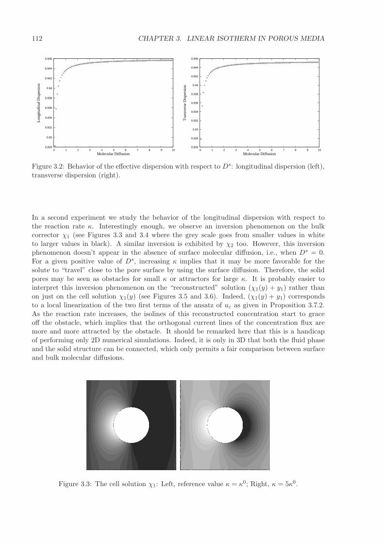
112 CHAPTER 3. LINEAR ISOTHERM IN POROUS MEDIA
0.828
0.83
0.832
0.834
0.836
0.838
0.84
0.842
0.844
0.846
0 1 2 3 4 5 6 7 8 9 10
Lon
gitu
dina
l Dis
pers
ion
Molecular Diffusion
0.826
0.828
0.83
0.832
0.834
0.836
0.838
0.84
0.842
0.844
0.846
0 1 2 3 4 5 6 7 8 9 10
Tra
nsve
rse
Dis
pers
ion
Molecular Diffusion
Figure 3.2: Behavior of the effective dispersion with respect to Ds: longitudinal dispersion (left),transverse dispersion (right).
In a second experiment we study the behavior of the longitudinal dispersion with respect tothe reaction rate κ. Interestingly enough, we observe an inversion phenomenon on the bulkcorrector χ1 (see Figures 3.3 and 3.4 where the grey scale goes from smaller values in whiteto larger values in black). A similar inversion is exhibited by χ2 too. However, this inversionphenomenon doesn’t appear in the absence of surface molecular diffusion, i.e., when Ds = 0.For a given positive value of Ds, increasing κ implies that it may be more favorable for thesolute to “travel” close to the pore surface by using the surface diffusion. Therefore, the solidpores may be seen as obstacles for small κ or attractors for large κ. It is probably easier tointerpret this inversion phenomenon on the “reconstructed” solution (χ1(y) + y1) rather thanon just on the cell solution χ1(y) (see Figures 3.5 and 3.6). Indeed, (χ1(y) + y1) correspondsto a local linearization of the two first terms of the ansatz of uε as given in Proposition 3.7.2.As the reaction rate increases, the isolines of this reconstructed concentration start to graceoff the obstacle, which implies that the orthogonal current lines of the concentration flux aremore and more attracted by the obstacle. It should be remarked here that this is a handicapof performing only 2D numerical simulations. Indeed, it is only in 3D that both the fluid phaseand the solid structure can be connected, which only permits a fair comparison between surfaceand bulk molecular diffusions.
Figure 3.3: The cell solution χ1: Left, reference value κ = κ0; Right, κ = 5κ0.

3.13. NUMERICAL STUDY 113
Figure 3.4: The cell solution χ1: Left, κ = 6κ0; Right, κ = 8κ0.
Figure 3.5: The reconstructed solution χ1(y)+y1: Left, Reference value κ = κ0; Right, κ = 6κ0.
Figure 3.6: The reconstructed solution χ1(y) + y1: Left, κ = 12κ0; Right, κ = 19κ0.
In Figures 3.7 and 3.8 we plot the dispersion in two asymptotic regimes: κ → 0 and κ → ∞.Once again when κ → ∞ we get an asymptote for the dispersion, corresponding to a limit cellproblem where Kχi = ωi. In this limit, the corresponding system satisfied by the bulk corrector

114 CHAPTER 3. LINEAR ISOTHERM IN POROUS MEDIA
χi is
b(y) · ∇yχi − divy(D(∇yχi + ei)) = (b∗ − b) · ei in Y 0,
−K−1D(∇yχi + ei) · n+ (b∗ − bs) · ei =
bs(y) · ∇syχi − divsy(D
s(∇syχi + ei)) on ∂Σ0,
y → χi(y) Y -periodic.
(3.116)
Of course, the transverse dispersion is always smaller than the longitudinal dispersion. Figures3.7 and 3.8 show the blow-up behavior of both longitudinal and transverse dispersions whenκ→ 0. This is due to the ill-posedness of the cell problem (3.31) in the limit κ→ 0.
0
20
40
60
80
100
120
140
160
180
200
220
0 1e-05 2e-05 3e-05 4e-05 5e-05 6e-05 7e-05 8e-05 9e-05 0.0001
Lon
gitu
dina
l Dis
pers
ion
Reaction Rate 1.55
1.6
1.65
1.7
1.75
1.8
1.85
0 50 100 150 200 250 300
Lon
gitu
dina
l Dis
pers
ion
Reaction Rate
Figure 3.7: Behavior of the longitudinal dispersion with respect to κ: when κ goes to 0 (left),when κ goes to infinity (right).
0.7768
0.77681
0.77682
0.77683
0.77684
0.77685
0.77686
0.77687
0.77688
0.77689
0 1e-05 2e-05 3e-05 4e-05 5e-05 6e-05 7e-05 8e-05 9e-05 0.0001
Tra
nsve
rse
Dis
pers
ion
Reaction Rate 0.3
0.35
0.4
0.45
0.5
0.55
0.6
0 50 100 150 200 250 300
Tra
nsve
rse
Dis
pers
ion
Reaction Rate
Figure 3.8: Behavior of the transverse dispersion with respect to κ: when κ goes to 0 (left),when κ goes to infinity (right).
3.14 Comments
Locally periodic coefficients
In this chapter we have analysed the reactive transport of a single solute in presence of adsorp-tion reaction on the pore boundaries. Bulk and solute concentrations were governed by coupled

3.14. COMMENTS 115
partial differential equations (3.11)-(3.13) with purely periodic coefficients i.e., bε(x) = b(x/ε),Dε(x) = D(x/ε). The obvious question would be:
Is it possible to relax the pure periodicity assumption on the coefficients in (3.11)-(3.13) andstill homogenize the microscopic model ?
We can give a partial answer to this question. As far as the diffusion matrices D and Ds go, wecan consider them to be locally periodic i.e., Dε(x) = D(x, x/ε), Ds
ε(x) = Ds(x, x/ε) and stillthe homogenization techniques used in this chapter to arrive at the effective equations apply.The dispersion D that we found in Section 3.7 is symmetric and constant. We symmetrizedthe expression for the dispersion during the process of upscaling as the Hessian matrix ∇2u0 issymmetric. In case of locally periodic diffusion matrices, however, we shouldn’t symmetrize theexpression for D.
So there is a possibility of relaxing the pure periodicity assumption on the diffusion coefficientsin (3.11)-(3.13). This doesn’t extend to the velocity fields in (3.11)-(3.13). We are working in thestrong convection regime. As we explained in Section 2.6 of Chapter 2, the classical two-scaleasymptotic expansion method had to be modified by taking large drift in the slow variable. Thismethod of two-scale asymptotic expansions with drift considers only constant values for drift.In the expression for the effective drift (3.27), if we blindly relax the pure periodicity conditionson the velocity fields then the drift velocity b∗ isn’t a constant and this is not admissible. This isone of the main technical reasons. Also the chain rule differentiation formulae (3.24) that we usewhile performing the formal calculations do not hold true anymore if b∗ weren’t a constant. Itis to be noted that under special assumptions on the coefficients, G. Allaire and R. Orive in [22]have shown that a new localization phenomenon can occur which is completely different fromthe asymptotic behaviour proved in this Chapter. This highlights the need for the developmentsof new tools in the theory of periodic homogenization.
Quantitative analysis
Quantification of the dispersion tensor is of crucial importance. In the regime of “strong con-vection”, some of the results on deriving upper and lower bounds for the dispersion tensor canbe found in [138]. In this Chapter we have found expressions for different effective parametersin terms of the local parameters. Even though in Section 3.13, we have attempted to study thebehaviour of those effective parameters with respect to local ones, it can be of value to pursuethe analysis to find optimal bounds on the effective parameters. There have been some astonish-ing works in this regard in the absence of chemical reactions [93], [119]. In the cited references,for example, it is proved that the dispersion increases or diminishes depending on whether themean value of the velocity field is rational or irrational. We could try to analyze if we arriveat those results in the limit of reaction rate going to zero. In the general introduction to thisthesis (Chapter 1), we gathered some results on the upscaling of reactive flows in “Diffusiondominated regime” [77], [97], [78], [79], [80], [81], [69], [68]. We could compare the effectiveparameters obtained in that regime with those obtained in this Chapter.
Random porous media
All through this Chapter we have worked with only periodic porous medium and periodic co-efficients. A. Bourgeat, A. Mikelic and S. Wright in [45] adapted the “two-scale convergencemethod” of periodic regime to random regimes under some suitable stationarity assumptions. Inthe large Peclet regime, we have learnt the need to modify the method of two-scale convergenceby the introduction of large drift in the slow variable. We can try to adapt this new notion of

116 CHAPTER 3. LINEAR ISOTHERM IN POROUS MEDIA
“two-scale convergence with drift” to random regimes in the spirit of [45]. If successful, we willbe able to find effective dispersion in large Peclet regime in random porous media. J. L. Auriaultin [32] argues that the random and periodic media present similar macroscopic description, whenit exists. So, the analysis of the system with randomly oscillating coefficients gets interesting.
Conclusions
Finally, this Chapter has analyzed all possible scenarios for the reactive transport of single solutein periodic regime in presence of linear reaction terms. We have also seen that we recover theprevious results in this regime of “strong convection” in various asymptotic regimes. In the nextChapter we move on to the homogenization problem related to a nonlinear adsorption isotherm.

Chapter 4
Langmuir isotherm in porous media
4.1 Introduction
As in Chapter 3, this chapter is devoted to the study of an adsorption process occurring at thesolid-fluid interface in an ε-periodic rigid porous medium. The novelty of the mesoscale modelconsidered in this chapter is the presence of nonlinear terms modelling the adsorption process asopposed to the linear case studied in Chapter 3. We will be working with a convection diffusionequation for the solute concentration in the bulk and a convection diffusion equation for theadsorbed concentration on the pores surface, both being coupled by a nonlinear reaction termmodeling the adsorption phenomena at the solid fluid interface. We shall get into the modellingand scaling aspects of the governing equations in Section 4.3. The presence of nonlinear termsalways gets interesting in the homogenization process. Starting with a linear coupled convec-tion diffusion reaction equations in Chapter 3, we arrived at a scalar linear diffusion equationin moving coordinates. In this chapter too, we shall be employing the method for two-scaleconvergence with drift [121] (recalled in Section 2.6) to derive the effective equation. It wouldbe of interest to study how the nonlinearities are going to affect the homogenization result. Thedrift velocity b∗ associated with the linear model (3.11)-(3.13) was shown to be equal to (3.27):
b∗ =
∫
Y 0
b(y) dy +K
∫
∂Σ0
bs(y) dσ(y)
|Y 0|+K|∂Σ0|d−1
.
The nonlinear isotherm (4.2) with which we will be working all through this chapter is that givenby Langmuir. An interesting exercise would be to derive an expression for the drift velocityassociated with the convection diffusion adsorption equations with the nonlinear isotherm (4.2).In Section 2.9, we remarked that the drift velocity b∗ in the method of two-scale convergencewith drift has to be independent of the slow variable x. This handicap of the method necessitatesa technical assumption, in the current case of Langmuir adsorption, on the velocity fields whichamounts to say that the bulk and surface drifts are equal (their common value being called b∗
in the sequel)
1
|Y 0|
∫
Y 0
b(y) dy =1
|∂Σ0|
∫
∂Σ0
bs(y) dσ(y) = b∗, (4.1)
where b(y) is a Y -periodic velocity field in the bulk Ωf and bs(y) is a Y -periodic velocity field onthe pores surface ∂Ωs. Such an assumption was not necessary in the linear case [10], [20], [17]but is the price to pay for extending our previous results to the nonlinear case of the Langmuirisotherm.
117

118 CHAPTER 4. LANGMUIR ISOTHERM IN POROUS MEDIA
Our main result (Theorem 4.8.1) says that the solution (uε, vε) of the coupled convection diffusionreaction system (4.12)-(4.14) is approximatively given by the ansatz
uε(t, x) ≈ u0
(t, x− b∗t
ε
)+ εu1
(t, x− b∗t
ε,x
ε
),
vε(t, x) ≈ f(u0)
(t, x− b∗t
ε
)+ εv1
(t, x− b∗t
ε,x
ε
),
where f is the Langmuir isotherm given in (4.2) and u0 is the solution of the following macro-scopic nonlinear monotone diffusion equation
[|Y 0|+ α|∂Σ0|
(1 + βu0)2
]∂u0∂t
− divx(D(u0)∇xu0) = 0 in (0, T ) × Rd,
[|Y 0|u0 +
|∂Σ0| α u01 + βu0
](0, x) = |Y 0|uin(x) + |∂Σ0|vin(x) in Rd,
and the correctors (u1, v1) are defined by
u1(t, x, y) =d∑
i=1
χi
(y, u0(t, x)
)∂u0∂xi
(t, x)
and
v1(t, x, y) =α
(1 + βu0(t, x))2
d∑
i=1
ωi
(y, u0(t, x)
)∂u0∂xi
(t, x)
where (χi, ωi)1≤i≤d is the solution of the cell problem
−b∗ · ei + b(y) · (ei +∇yχi)− divy(D(ei +∇yχi)) = 0 in Y 0,
−D (ei +∇yχi) · n =ακ
(1 + βu0)2(χi − ωi) on ∂Σ0,
−b∗ · ei + bs(y) · (ei +∇syωi)− divsy(D
s(ei +∇syωi)) = κ (χi − ωi) on ∂Σ0,
y → (χi(y), ωi(y)) Y − periodic.
Note that the cell solution (χ, ω) depends not only on y but also on the value of u0(t, x).Furthermore, the technical assumption (4.1) is precisely the compatibility condition for solvingthe cell problem for any value of u0(t, x). In Chapter 3, the effective dispersion that we obtainedwas a constant and our upscaling method could only capture the symmetric part of the dispersionmatrix. In the nonlinear case, however, the effective diffusion (or dispersion) tensor D(u0) isgiven by
Dij(u0) =
∫
Y 0
D(y) (∇yχi + ei) · (∇yχj + ej) dy +ακ
(1 + βu0)2
∫
∂Σ0
[χi − ωi] [χj − ωj] dσ(y)
+α
(1 + βu0)2
∫
∂Σ0
Ds(y)(∇s
yωi + ei)·(∇s
yωj + ej)dσ(y)
+
∫
Y 0
D(y)(∇yχj · ei −∇yχi · ej
)dy
+α
(1 + βu0)2
∫
∂Σ0
Ds(y)(∇s
yωj · ei −∇syωi · ej
)dσ(y)
+
∫
Y 0
(b(y) · ∇yχi
)χj dy +
α
(1 + βu0)2
∫
∂Σ0
(bs(y) · ∇s
yωi
)ωj dσ(y)
4.2. LANGMUIR’S ADSORPTION ISOTHERM 119
which is neither symmetric nor constant. The presence of nonlinear terms in the mesoscopicequation has led to an effective behavior where the cell problem and the homogenized equationare explicitly coupled as shown by the above given expressions.
This chapter is outlined as follows. Section 4.2 introduces the Langmuir isotherm extensivelyused in surface chemistry and also recalls Freundlich isotherm. Having introduced the relevantisotherm that governs the chemical phenomena, in Section 4.3 we take up the task of mathe-matical modeling. The equations that govern the coupled phenomena of interest are rescaled toarrive at the mesoscopic system (4.12)-(4.14). Section 4.4 deals with the maximum principles(see Proposition 4.4.1) and a priori estimates for (4.12)-(4.14) which are obtained via energyestimates (see Lemma 4.4.2). Section 4.5 concerns itself with the wellposedness nature of thesystem (4.12)-(4.14). Finite dimensional Galerkin approximation method is employed in show-ing the existence of the solutions (uε, vε) for (4.12)-(4.14). The main result of Section 4.5 isProposition 4.5.1, the proof of which goes via various lemmata that are proved in Section 4.5and relies on the monotone character of the nonlinear Langmuir isotherm. After the qualitativeanalysis of Sections 4.4 and 4.5, we shall get into the crux of the objective i.e., the homoge-nization of the mesoscopic model (4.12)-(4.14). The nonlinearity of (4.12)-(4.14) requires somestrong compactness of the sequence of solutions in order to pass to the limit. This shall be thegoal of Section 4.6. The needed strong compactness result is obtained in Corollary 4.6.7 which isthe most technical result of the present chapter. Following the ideas of [121], [24], we first showthat, in a moving frame of reference, a uniform localization of solutions holds (Lemma 4.6.1).Then a time equicontinuity type result (Lemma 4.6.2) allows us to gain compactness. Thesetechnical results are not straightforward extensions of those in [121], [24]. There are a numberof additional difficulties, including the perforated character of the domain, the nonlinearity ofthe equations and more importantly the fact that there are two unknowns uε and vε. Section4.7 is dedicated to the extraction of converging subsequences of the solution sequences. In thissection, we intensely use the relative compactness results of Sections 2.6 and 2.7 from Chapter2. The derivation of the homogenized equation is left to Section 4.8 (Theorem 4.8.1) using themethod of two-scale convergence with drift [121], [7]. Theorems 4.7.2 and 4.8.1 give a result ofweak convergence of the sequence (uε, vε) to the homogenized limit (u0, v0 = f(u0)). Althoughthe previous Corollary 4.6.7 gives some strong compactness in the L2-norm, there is still roomto improve the strong convergence, notably for the gradients of uε and vε. This is the purposeof Section 4.9 where we establish a strong convergence result (Theorem 4.9.1) for well preparedinitial data. Eventually, Section 4.10 is devoted to some 2D numerical simulations using theFreeFem++ package [141]. In the 2D setting, assumption (4.1) implies that the homogenizeddrift vanishes, i.e., b∗ = 0. We study the behaviour of the homogenized dispersion tensor withrespect to variations of the magnitude of u0, the reaction rate κ and the surface moleculardiffusion Ds. We also plot the homogenized solution u0 and the reconstructed solution
uε(t, x) = u0(t, x) + ε
d∑
i
χi
(xε, u0
)∂u0∂xi
(t, x)
to see the importance of the corrector term. Finally, in Section 4.11, we make some observationson the calculations done along this chapter and compare the results obtained in this chapterwith those of Chapter 3 in the linear setting.
4.2 Langmuir’s adsorption isotherm
Upon presenting the Henry’s adsorption isotherm (linear) in Section 3.2, we did give expressionsfor a couple of known nonlinear isotherms (3.3) and (3.4). One among them is the following

120 CHAPTER 4. LANGMUIR ISOTHERM IN POROUS MEDIA
Langmuir isotherm.
f(u) =αu
1 + βuwith α, β > 0 (4.2)
The primitive of the Langmuir isotherm (4.2) is given by
F (uε) =α
β
[uε −
1
βlog(1 + βuε)
](4.3)
The primitive (4.3) vanishes at zero. In [111], Langmuir gave a description of the equilibriumbetween a single component gas and the adsorbed species at a surface. He gave a relationshipbetween the fraction of the surface covered by adsorbed species, θg , and the partial pressure ofthe single component gas exposed to the surface, pg.
θg =αpg
1 + βpg(4.4)
The above expression can be obtained by the mass-action kinetics as demonstrated in Chapter11 of [102]. In case of liquid-solid interface, we shall replace the partial pressure by concentrationof the solute dissolved in the liquid phase and the surface fraction by the concentration of theadsorbed solute. Let u be the concentration of the dissolved solute in the bulk and v be theconcentration of the same solute in the adsorbed state in the interface. Then, at chemicalequilibrium we have
v = f(u). (4.5)
As the interest is to study the non equilibrium reactions, we consider the following ordinarydifferential equation for the adsorbed concentration.
dv
dt= κ(f(u)− v) with κ a positive constant. (4.6)
Another popular adsorption isotherm considered in the chemistry literature is due to Freundlich[88].
f(u) = αuβ with α > 0 and 0 < β < 1. (4.7)
The expressions (4.2) and (4.7) for the two isotherms have been used quite extensively in theliterature. However, the determination of the reaction coefficients is quite tedious and very casespecific. In order to simplify the mathematical analysis, there was an attempt made in [78] tojustify these two isotherms and generalize their notions. According to the cited reference, thereare two kinds of concave isotherms : Langmuir and Freundlich. A function f(u) is said to be of“Langmuir type” if it is strictly concave near u = 0 and f ′(0+) < +∞. The isotherm expressiongiven in (4.2) indeed falls into this category. On the other hand, f(u) is said to be of “Freundlichtype” if it is strictly concave near u = 0 and f ′(0+) = +∞. An example of one such isothermis (4.7).
4.3 Mathematical model
Let us consider an ε-periodic porous medium saturated with an incompressible fluid. Solutesof a kind are assumed to be dissolved in the fluid. The objective is to study the transport ofthe dissolved solutes. As in Chapter 3, we shall be considering transport both in the bulk ofthe fluid and on the porous skeleton.So we introduce two velocity fields: b(y) in the bulk of thefluid Ωf and bs(y) on the surface of the pores ∂Ωs. We shall not be analyzing any governingequations for these two velocity fields. Our hypothesis on these incompressible velocity fields

4.3. MATHEMATICAL MODEL 121
is that they are given, independent of time and Y -periodic. The incompressibility condition onboth the velocity fields means
divy b(y) = 0 and divsybs(y) = 0. (4.8)
We make the following regularity assumption on both velocity fields: b(y) ∈ L∞# (Ωf ;R
d), bs(y) ∈L∞# (∂Ωs;R
d) and bs = Gbs is always tangential to the surface whereG(y) is the projection matrixon the tangent hyperplane to the surface ∂Ωf = ∂Ωs. The molecular diffusion associated withthe dissolved solute is assumed to be periodic and different in bulk and on the surface. So, twoperiodic symmetric tensors D(y) ∈ L∞
# (Ωf )d×d and Ds(y) ∈ L∞
# (∂Ωs)d×d which are assumed to
be uniformly coercive, namely there exists a constant C > 0 such that, for any ξ ∈ Rd,
D(y)ξ · ξ ≥ C|ξ|2 a.e. in Ωf , Ds(y)ξ · ξ ≥ C|ξ|2 a.e. on ∂Ωs.
are introduced. The solutes in the bulk of the fluid are subjected to transport via the convectivefield b(y) and they diffuse in the bulk, thanks to the associated diffusion matrix D(y). Theequation that models this combined phenomena is the following convection diffusion equationfor u, the solute concentration in the fluid bulk.
∂u
∂τ+ b · ∇u− div (D∇u) = 0 in (0, ζ)× Ωf (4.9)
As recalled in the introduction, we wish to study the transport of the adsorbed concentrationtoo as in Chapter 3. Let v to the concentration of the adsorbed solutes in the interface. InSection 4.2, we have introduced an ordinary differential equation (4.6) that represents the nonequilibrium chemical phenomena in terms of an isotherm. The presence of surface convectivefield bs and the surface diffusion Ds associated with the solute modify (4.6) into the followingpartial differential equation.
∂v
∂τ+ bs · ∇sv − divs (Ds∇sv) = κ
( αu
1 + β u− v)
on (0, ζ) × ∂Ωs. (4.10)
To balance the mass of the system, we shall impose the right hand side of (4.10) as Neumannboundary data for u on the skeleton ∂Ωs.
−D∇u · n = κ( αu
1 + β u− v)
on (0, ζ)× ∂Ωs (4.11)
The above system (4.9)-(4.11) is also supplemented with initial data. Our goal is to study thehomogenization problem in the strong convection regime. So, we shall parabolically scale thesystem (4.9)-(4.11) i.e., by making the following change of variables: (τ, y) → (ε−2t, ε−1x). Theresulting adimensionalized coupled convection diffusion reaction equations for the new unknownsuε(t, x) = u(τ, y) and vε(t, x) = v(τ, y) are given by
∂uε∂t
+1
εbε · ∇uε − div (Dε∇uε) = 0 in (0, T ) × Ωε (4.12)
−Dε
ε∇uε · n =
∂vε∂t
+1
εbsε · ∇svε − divs (Ds
ε∇svε) =κ
ε2
( αuε1 + βuε
− vε
)on (0, T ) × ∂Ωε (4.13)
uε(0, x) = uin(x) in Ωε, vε(0, x) = vin(x) on ∂Ωε (4.14)
for some final time T = ε2ζ. As ζ = O(ε−2), the final time T is indeed of O(1). The initial dataare chosen such that uin(x) ∈ L2(Rd) and vin(x) ∈ H1(Rd) (so that its trace is well-defined on∂Ωε). Remark that the coefficients in (4.12)-(4.13) are all ε-periodic with the following notations:Dε(x) = D(x/ε), Ds
ε(x) = Ds(x/ε), bε(x) = b(x/ε) and bsε(x) = bs(x/ε).

122 CHAPTER 4. LANGMUIR ISOTHERM IN POROUS MEDIA
4.4 Maximum principles and a priori estimates
We use the standard notations h+ = max(0, h) and h− = min(0, h). Recall that the functionf(u) = αu/(1 + βu) is one to one and increasing from R+ to [0, α/β]. Although the functionf(u) is not defined for u = −1/β, and since we are interested only in non negative values ofu, we can modify and mollify f(u) as we wish for u < 0 so that it is an increasing functionon R and all computations below make sense for negative values of u. Next, we give a resultin the spirit of proving some maximum principles for (4.12)-(4.14). This result is analogous toProposition 3.5.1 of Chapter 3. The objective of the next result is to assert that the solution(uε, vε) to (4.12)-(4.13) remains non negative and bounded if one prescribes non negative andbounded initial data (uin, vin) in (4.14).
Proposition 4.4.1. Let (uε, vε) be a weak solution of (4.12)-(4.14). Assume that the initialdata (uin, vin) satisfy 0 ≤ uin ≤ Mu, 0 ≤ vin ≤ Mv for some positive constants Mu and Mv
(without loss of generality consider f(Mu) < Mv).
If Mv < α/β, then
0 ≤ uε(t, x) ≤ mu = f−1(Mv) for (t, x) ∈ (0, T ) × Ωε,0 ≤ vε(t, x) ≤Mv for (t, x) ∈ (0, T ) × ∂Ωε.
(4.15)
If Mv ≥ α/β, then there exist three positive constants τ , M(τ) and Mv < α/β, independent ofε, such that
0 ≤ uε(t, x) ≤M(τ) for (t, x) ∈ (0, ε2τ)× Ωε,0 ≤ vε(t, x) ≤Mv for (t, x) ∈ (0, ε2τ)× ∂Ωε,
(4.16)
and 0 ≤ uε(t, x) ≤ mu = f−1(Mv) for (t, x) ∈ (ε2τ, T )× Ωε,
0 ≤ vε(t, x) ≤ Mv for (t, x) ∈ (ε2τ, T )× ∂Ωε.(4.17)
Proof. As was done in the proof of Proposition 3.5.1, we shall be using a variational approach.To begin with, we prove that the solutions remain non negative for non negative initial data.Let us consider (f(uε)
−, εv−ε ) as test functions in the variational formulation of (4.12)-(4.14).
T∫
0
d
dt
∫
Ωε
F (u−ε ) dx dt+1
ε
T∫
0
∫
Ωε
bε · ∇F (u−ε ) dx dt−T∫
0
∫
Ωε
div (Dε∇uε) f(uε)− dx dt
+ε
2
T∫
0
d
dt
∫
∂Ωε
|v−ε |2 dσ(x) dt+ε
2
T∫
0
∫
∂Ωε
bsε · ∇s|v−ε |2 dσ(x) dt
−εT∫
0
∫
∂Ωε
divs (Dsε∇svε) v
−ε dσ(x) dt −
κ
ε
T∫
0
∫
∂Ωε
[f(uε)− vε] v−ε dσ(x) dt = 0 (4.18)
where f and its primitive F are defined by (4.2) and (4.3) respectively. The divergence freeassumption on the velocity fields b, bs and the non-penetrating boundary conditions for b on theporous skeleton result in the vanishing of the convective terms in the variational formulation(4.18). Thus, we get
∫
Ωε
F (u−ε )(T ) dx+ε
2
∫
∂Ωε
|v−ε (T )|2 dσ(x) +T∫
0
∫
Ωε
f ′(u−ε )Dε∇u−ε · ∇u−ε dx dt

4.4. MAXIMUM PRINCIPLES AND A PRIORI ESTIMATES 123
+ε
T∫
0
∫
∂Ωε
Dsε∇sv−ε · ∇sv−ε dσ(x) dt+
κ
ε
T∫
0
∫
∂Ωε
(f(uε)− vε
)(f(uε)
− − v−ε
)dσ(x) dt
=
∫
Ωε
F (u−ε )(0) dx +ε
2
∫
∂Ωε
|v−ε (0)|2 dσ(x) (4.19)
The function h → h− is monotone and we know that f ′(u) > 0. So, each one of the terms onthe left hand side of (4.19) are positive. The assumption of the non negative initial data impliesthat the right hand side of (4.19) vanishes thus resulting in
u−ε (t, x) = 0 and v−ε (t, x) = 0 for all times t ∈ (0, T ]. (4.20)
Next, we show that the solutions stay bounded from above if we start with a bounded initialdata. The boundedness property of f adds an additional difficulty prompting us to consider twocases as below.Case I. Assume Mv < α/β so we can define mu = f−1(Mv) > Mu.We choose ((f(uε)−Mv)
+, ε(vε−Mv)+) as test functions in the variational formulation of (4.12)-
(4.14). Introducing the primitive function F such that F ′(u) = (f(u)−Mv)+ and F(0) = 0, we
get
∫
Ωε
F(uε)(T ) dx +ε
2
∫
∂Ωε
|(vε −Mv)+|2 dσ(x) +
T∫
0
∫
Ωε
f ′(uε)Dε∇(uε −mu)+ · ∇(uε −mu)
+ dx dt
+ε
T∫
0
∫
∂Ωε
Dsε∇s(vε −Mv)
+ · ∇s(vε −Mv)+ dσ(x) dt
+κ
ε
T∫
0
∫
∂Ωε
((f(uε)−Mv)− (vε −Mv)
)((f(uε)−Mv)
+ − (vε −Mv)+)dσ(x) dt
=
∫
Ωε
F(uin) dx+ε
2
∫
∂Ωε
((vin −Mv)+)2 dσ(x), (4.21)
because ∇(f(uε) −Mv)+ = f ′(uε)∇(uε −mu)
+. The upper bound on the initial data impliesthat the right hand side in (4.21) vanishes. The left hand side is non-negative because h→ h+ ismonotone and f ′(uε) ≥ 0. Since F(u) = 0 if and only if u ≤ mu, we deduce (4.16) that uε ≤ mu
and vε ≤Mv.Case II. Assume Mv ≥ α/β.The argument in Case I fails here because f−1(Mv) is not well defined. The idea is to first provethat there exists τ > 0 such that, after a short time ε2τ , the solution vε reduces in magnitudeand is uniformly smaller than α/β. Then by taking ε2τ as a new initial time we can repeat theanalysis of Case I. Whatever the value of uε, equation (4.13) implies the following inequality onthe boundary ∂Ωε
∂vε∂t
+1
εbsε · ∇svε − divs (Ds
ε∇svε) ≤κ
ε2
(αβ− vε
). (4.22)
Choosing qε =
(vε −
α
β
)exp(tκ/ε2) we get
∂qε∂t
+1
εbsε · ∇sqε − divs (Ds
ε∇sqε) ≤ 0

124 CHAPTER 4. LANGMUIR ISOTHERM IN POROUS MEDIA
with the initial data
qε(0) = vin − α
β.
Then, the maximum principle implies (see [143] for details)
qε(t) ≤ maxx∈∂Ωε
qε(0) ≤Mv −α
β,
which yields the following upper bound
vε(t) ≤ exp(−tκ/ε2)Mv +(1− exp(−tκ/ε2)
)αβ. (4.23)
Unfortunately (4.23) is too crude a bound which cannot reduce the initial boundMv to a numbersmaller than α/β. At least, (4.23) yields vε(t) ≤ Mv. We are going to use this upper bound inthe equation for uε in order to improve (4.23).
Equations (4.12) and (4.13) give the following equation for uε
∂uε∂t
+1
εbε · ∇uε − div (Dε∇uε) = 0 in Ωε,
−Dε
ε∇uε · n =
κ
ε2
( αuε1 + βuε
− vε
)=
κ
ε2gε on ∂Ωε,
(4.24)
with gε satisfying, thanks to (4.23), the bound |gε| ≤Mv. Let us introduce an auxiliary problemin the unit cell
b(y) · ∇yΨ− divy(D(y)∇yΨ) = κMv |∂Σ0|/|Y 0| in Y 0,
−D(y)∇yΨ · n = κMv on ∂Σ0,
y → Ψ(y) is Y -periodic,
(4.25)
where the compatibility condition for the existence and uniqueness (up to an additive constant)of Ψ is satisfied. The scaled function Ψε(x) = Ψ(x/ε) satisfies
1
εbε · ∇Ψε − div(Dε∇Ψε) =
κMv
ε2|∂Σ0|/|Y 0| in Ωε,
−1
εDε∇Ψε · n =
κMv
ε2on ∂Ωε.
(4.26)
Let us define a function
pε = Ψε + uε −(κMv
ε2|∂Σ0|/|Y 0|
)t (4.27)
Then, pε satisfies
∂pε∂t
+1
εbε · ∇pε − div (Dε∇pε) = 0 in (0, T )× Ωε,
−1
εDε∇pε · n =
κ
ε2(gε +Mv) ≥ 0 on (0, T ) × ∂Ωε,
pε(0, x) = Ψε(x) + uin(x) in Ωε.
(4.28)
Then, the maximum principle yields (again see [143] if necessary)
pε(t) ≤ maxΩε
(Ψε + uin) ≤Mu + ‖Ψ‖L∞(Y 0). (4.29)

4.4. MAXIMUM PRINCIPLES AND A PRIORI ESTIMATES 125
From the definition (4.27) of pε we deduce
uε(t) ≤Mu + 2‖Ψ‖L∞(Y 0) +κMv
ε2|∂Σ0|/|Y 0|t, (4.30)
which implies that, for any τ > 0, we have
max0<t<ε2τ
uε(t) ≤M(τ) =Mu + 2‖Ψ‖L∞(Y 0) + κMv |∂Σ0|/|Y 0|τ, (4.31)
where M(τ) does not depend on ε and is an affine function of τ . Hence
max0<t<ε2τ
f(uε(t)) ≤ f(M(τ)) =αM(τ)
1 + βM(τ)<α
β(4.32)
and (4.22) can be improved as
∂vε∂t
+1
εbSε · ∇Svε − divS
(DS
ε ∇Svε)≤ κ
ε2
(f(M(τ))− vε
)for 0 < t < ε2τ.
The same argument leading to (4.23) now gives that, for any τ > 0 and 0 < t < ε2τ ,
vε(t) ≤ exp(−κτ)Mv +(1− exp(−κτ)
)f(M(τ)), (4.33)
where f(M(τ)) < αβ − C
τ for some positive constant C > 0. Thus, choosing τ large enough, we
deduce that there exists Mv (equal to the right hand side of (4.33)) which does not depend onε such that
max0<t<ε2τ
vε(t) ≤ Mv <α
β. (4.34)
Choosing Mu =M(τ), we obviously have f(Mu) < Mv and we can repeat the argument of CaseI with the new initial time ε2τ .
Proposition 4.4.1 implied that the solutions to (4.12)-(4.14) are bounded in the L∞-norm. Thisinformation shall come in handy while deriving a priori estimates on the solution (uε, vε). Next,we state a lemma that gives the a priori estimates on the solution to our mesoscopic model.
Lemma 4.4.2. Let (uε, vε) be a weak solution of (4.12)-(4.14) and the initial data (uin, vin) besuch that 0 ≤ uin ≤Mu, 0 ≤ vin ≤Mv. There exists a constant C that depends on Mu and Mv
but not on ε such that
‖uε‖L∞((0,T );L2(Ωε)) +√ε‖vε‖L∞((0,T );L2(∂Ωε))
+‖∇uε‖L2((0,T )×Ωε) +√ε‖∇svε‖L2((0,T )×∂Ωε)
+√ε‖wε‖L∞((0,T );L2(∂Ωε)) ≤ C
(∥∥uin∥∥L2(Rd)
+ ‖vin‖H1(Rd)
),
(4.35)
where wε = ε−1
(αuε
1 + βuε− vε
).
Proof. To obtain an energy equality we multiply (4.12) by f(uε) and integrate over Ωε
d
dt
∫
Ωε
F (uε) dx+
∫
Ωε
f ′(uε)Dε∇uε · ∇uε dx+κ
ε
∫
∂Ωε
(f(uε)− vε) f(uε) dσ(x) = 0,

126 CHAPTER 4. LANGMUIR ISOTHERM IN POROUS MEDIA
where F is the primitive of f , defined by (4.3), which satisfies F (u) ≥ 0 for u ≥ 0. We nextmultiply (4.13) by εvε and integrate over ∂Ωε
ε
2
d
dt
∫
∂Ωε
|vε|2 dσ(x) + ε
∫
∂Ωε
Dsε∇svε · ∇svε dσ(x)−
κ
ε
∫
∂Ωε
(f(uε)− vε) vε dσ(x) = 0.
Adding the above two expressions leads to the following energy equality
d
dt
∫
Ωε
F (uε) dx+ε
2
d
dt
∫
∂Ωε
|vε|2 dσ(x) +∫
Ωε
f ′(uε)Dε∇uε · ∇uε dx
+ε
∫
∂Ωε
Dsε∇svε · ∇svε dσ(x) +
κ
ε
∫
∂Ωε
(f(uε)− vε)2 dσ(x) = 0. (4.36)
Recalling that, because of the maximum principle of Proposition 4.4.1, F (uε) ≥ 0 and f ′(uε) ≥ 0,and integrating over time yields
‖F (uε)‖L∞((0,T );L1(Ωε))+ ε‖vε‖2L∞((0,T );L2(∂Ωε))
+ ε
∥∥∥∥1
ε(f(uε)− vε)
∥∥∥∥2
L2(∂Ωε×(0,T ))
+∥∥∥√f ′(uε)∇uε
∥∥∥2
L2(Ωε×(0,T ))+ ε‖∇svε‖2L2(∂Ωε×(0,T )) ≤ C
(∥∥F (uin)∥∥L1(Rd)
+ ‖vin‖2H1(Rd)
)
(4.37)A second-order Taylor expansion at 0 yields F (u) = 1
2u2f ′(c) for some c ∈ (0, u). By the
maximum principle we have 0 ≤ uε ≤M so that
0 <α
1 + βM≤ f ′(uε) ≤ α, (4.38)
and∥∥F (uin)
∥∥L1(Rd)
≤ C∥∥uin
∥∥2L2(Rd)
while
‖F (uε)‖L∞((0,T );L1(Ωε))+∥∥∥√f ′(uε)∇uε
∥∥∥2
L2(Ωε×(0,T ))≥ C
(‖uε‖2L∞((0,T );L2(Ωε))
+ ‖∇uε‖2L2(Ωε×(0,T ))
)
(4.39)from which we deduce (4.35).
4.5 Existence and uniqueness
Establishing the wellposedness of the coupled system (4.12)-(4.14) follows by the argumentsof the finite dimensional Galerkin approximations [110], [114], [115], [84]. We shall be takingsome cues from [127] where an adsorption/desorption model is studied in a different geometricand chemical setting. The method of finite Galerkin approximations, as the name suggests,is to construct finite dimensional approximations to the solution. After constructing the finitedimensional approximations, we shall tend the dimensions of the approximation spaces to infinityhoping to find a limit. The next step shall be to show that the limit does exist. The final stepwould be to prove that the limit is, indeed, the solution that we are looking for. The presenceof the nonlinear terms in (4.12)-(4.14) dictate the need for strong compactness type results inorder to pass to the limit. Additional difficulty arises due to the unbounded nature of our porousdomain Ωε as the Rellich’s theorem doesn’t apply. So we shall construct a sequence uN,A
ε offinite dimensional approximations to the solution where A is the size of a bounded cube inRd and N is the dimension of the finite dimensional approximation space. As a first step, we

4.5. EXISTENCE AND UNIQUENESS 127
shall keep A fixed and prove that uN,Aε attains a limit uAε as N → ∞. To this effect, we shall
derive a priori estimates on the time derivative of the approximate solutions in order to applyAubin’s lemma [31], [114]. Our next step would be to consider the sequence uAε and provethat it is relatively compact in L2((0, T ) × Ωε). As the ε-periodic porous medium Ωε that weare considering is unbounded, we need to prove a localization result in the following sense: fora given δ > 0, we can find a cube QR(δ) =] − R(δ),+R(δ)[d⊂ Rd such that the L2-norm of uAεis inferior to δ outside the cube QR(δ) for every A > R(δ). After obtaining the compactnessof the sequence of approximate solutions, we pass to the limit in the variational formulation asA → ∞. Thus, we will be able to prove the wellposedness result for (4.12)-(4.14). Proposition4.5.1 states this result on existence and uniqueness of the solution.
The limits considered in this section are N → ∞ and A→ ∞ where N is the dimension of thefinite dimensional approximation space and A is the size of a bounded cube in Rd. In the presentsection the scale parameter ε is fixed. The compactness is obtained in a fixed frame of reference.Section 4.6 is concerned with the study of the limit ε → 0 where we obtain compactness resultin a moving frame of reference. It is to be noted that the results in this section and the nextsection may look similar at a passing glance. But both are, in essence, quite different.
Proposition 4.5.1. Assume that the initial data (uin, vin) belong to the space L2(Rd)∩L∞(Rd)×H1(Rd) ∩ L∞(Rd) and are non negative. For any given ε > 0, there exists a unique solution(uε, vε) of (4.12)-(4.14) in the energy space, namely
uε ∈ L∞((0, T );L2(Ωε)), ∇uε ∈ L2((0, T ) × Ωε),
and
vε ∈ L∞((0, T );L2(∂Ωε)), ∇svε ∈ L2((0, T ) × ∂Ωε).
Before we give the proof for the Proposition 4.5.1, we shall prepare the ground work for theproof. To begin with, we shall adopt an approach from (Chapter 1, Section 6 of [114]) in thecontext of proving existence of solutions for unsteady Navier-Stokes equations. Let us considerthe following spectral problem
−∆ϕ+ ϕ = λϕ in Ωε ∩QA
−∇ϕ · n = 0 on ∂Ωε ∩QA
(4.40)
with periodic boundary conditions on ∂QA where QA =] − A,+A[d⊂ Rd is a cube. Associ-ated with (4.40) we have a sequence of eigenfunctions ϕε
jj∈N corresponding to a sequence ofeigenvalues λjj∈N:
∫
Ωε∩QA
(∇ϕε
j · ∇θ + ϕεjθ)dx = λj
∫
Ωε∩QA
ϕεjθ dx for θ ∈ H1
#(Ωε ∩QA), λj > 0. (4.41)
We shall be using ϕεjj∈N as basis functions to construct finite dimensional approximation
spaces for the bulk concentration uε. As done in (4.40) and (4.41), we shall be introducinganother set of basis eigenfunctions with the help of Laplace Beltrami operator to approximatethe surface concentration vε. Consider the sequence of eigenfunctions ψε
jj∈N corresponding toa sequence of eigenvalues νjj∈N obtained via
∫
∂Ωε∩QA
(∇sψε
j · ∇sΘ+ ψεjΘ)dσ(x) = νj
∫
∂Ωε∩QA
ψεjΘ dσ(x) for Θ ∈ H1
#(∂Ωε ∩QA), νj > 0.
(4.42)
128 CHAPTER 4. LANGMUIR ISOTHERM IN POROUS MEDIA
Let us consider the following finite dimensional subspaces of H1(Ωε ∩QA)
DNε = spanϕε
1, ϕε2, · · · , ϕε
N (4.43)
and that of H1(∂Ωε ∩QA)BN
ε = spanψε1, ψ
ε2, · · · , ψε
N. (4.44)
Consider the L2 projection PN from H1(Ωε ∩QA) to DNε i.e.,
PNw =
N∑
i=1
( ∫
Ωε∩QA
wϕεi dx
)ϕεi for w ∈ H1(Ωε ∩QA). (4.45)
Similarly consider the L2 projection PN from H1(∂Ωε ∩QA) to BNε i.e.,
PNw =N∑
i=1
(ε
∫
∂Ωε∩QA
wψεi dx
)ψεi for w ∈ H1(Ωε ∩QA). (4.46)
Thanks to the orthonormal property of ϕεj in L2, the operator norm of the projection PN
‖PN‖L(H1,DNε ) = inf
w 6=0
‖PNw‖L2
‖w‖H1
≤ 1. (4.47)
We define (uN,Aε (t), vN,A
ε (t)) ∈ DNε × BN
ε an approximate solution of order N to (4.12)-(4.14)posed in (0, T )× Ωε ∩QA as
uN,Aε (t, x) =
N∑
j=1
cN,Aj (t)ϕε
j(x), vN,Aε (t, x) =
N∑
j=1
dN,Aj (t)ψε
j (x), (4.48)
∫
Ωε∩QA
∂uN,Aε
∂tu dx+
1
ε
∫
Ωε∩QA
bε · ∇uN,Aε u dx+
∫
Ωε∩QA
Dε∇uN,Aε · ∇u dx
+ε
∫
∂Ωε∩QA
∂vN,Aε
∂tv dσ(x) +
∫
∂Ωε∩QA
bsε · ∇svN,Aε v dσ(x)
+ε
∫
∂Ωε∩QA
Dsε∇svN,A
ε · ∇sv dσ(x) +κ
ε
∫
∂Ωε∩QA
(f(uN,A
ε )− vN,Aε
)(u− v
)dσ(x) = 0 (4.49)
for every (u, v) ∈ DNε × BN
ε . The Fourier coefficients cN,Aj and dN,A
j in (4.48) do depend onthe scaling parameter ε. As far as the purpose of the wellposedness result (Proposition 4.5.1)is concerned, we have a fixed ε > 0. Not to complicate the notation for the Fourier coefficients,we shall not mention explicitly their dependence on ε but shall admit that they do. The aboveCauchy problem (4.49) is supplemented with initial data that are nothing but the projectionsof the initial data (uin, vin) on to the finite dimensional space:
uN,Aε (0) = PNu
in and vN,Aε (0) = PNv
in. (4.50)
Upon applying the classical Cauchy-Lipschitz-Picard theorem [66], the existence of a continu-ously differentiable solution (cN,A
j (t), dN,Aj (t)) on [0, Tm] for the Cauchy problem (4.49) follows.
The interval of existence [0, Tm] as given by the Cauchy-Lipschitz-Picard theorem forces us toshow that Tm is indeed T . The maximum principles that we obtained on the weak solutions

4.5. EXISTENCE AND UNIQUENESS 129
of (4.12)-(4.14) in Proposition 4.4.1 carry on to the approximate solutions (uN,Aε , vN,A
ε ) as well.Next, we shall state a lemma giving a priori estimates on the finite dimensional approximations(uN,A
ε , vN,Aε ). The proof follows line to line the same arguments as in Lemma 4.4.2 where we ob-
tained the a priori estimates on the solution (uε, vε). As usual variational approach is employedand the proof goes via the derivation of the energy estimate. So, we will simply state the resultgiving the a priori estimates on the approximations with no proof.
Lemma 4.5.2. Let (uN,Aε , vN,A
ε )N∈N be the finite dimensional approximations to the solution(uε, vε) for (4.12)-(4.14) posed in (0, T ) × Ωε ∩QA. Let us choose the initial data (uin, vin) tobe non negative and bounded. Then, there exists a constant C depending on the bounds of theinitial data but not on N such that
‖uN,Aε ‖L∞((0,T );L2(Ωε∩QA)) +
√ε‖vN,A
ε ‖L∞((0,T );L2(∂Ωε∩QA))
+‖∇uN,Aε ‖L2((0,T )×Ωε∩QA) +
√ε‖∇svN,A
ε ‖L2((0,T )×∂Ωε∩QA)
+√ε‖wN,A
ε ‖L∞((0,T );L2(∂Ωε∩QA)) ≤ C(∥∥uin
∥∥L2(Rd)
+ ‖vin‖H1(Rd)
),
(4.51)
where wN,Aε = ε−1
(αuN,A
ε
1 + βuN,Aε
− vN,Aε
).
The a priori estimates (4.51) imply that the energy associated with (4.49) is bounded and anypossibility of a blow up of the solutions at time Tm doesn’t arise. Thus the existence of solution(cN,A
j (t), dN,Aj (t)) on [0, T ] for any time T <∞. As explained in the beginning of this section the
idea here is to tend N towards infinity in order to arrive at a solution (uε, vε) of (4.12)-(4.14).The estimates from (4.51) helps us extract convergent subsequences off uN,A
ε and vN,Aε . But
the presence of the nonlinear term f in (4.49) demands strong compactness for uN,Aε . So, in
addition to the a priori estimates (4.51), we shall look for an a priori estimate on the timederivative of uN,A
ε . As only uN,Aε appears as an argument in the nonlinear term of (4.49), we
shall try to obtain a strong compactness result for uN,Aε N∈N. So let us take the test function v
to be zero in (4.49). Then using the projection PN , the Cauchy problem (4.49) can be rewrittenas ∫
Ωε∩QA
∂uN,Aε
∂tPNu dx+
1
ε
∫
Ωε∩QA
bε · ∇uN,Aε PNu dx
+
∫
Ωε∩QA
Dε∇uN,Aε · ∇PNu dx+
κ
ε
∫
∂Ωε∩QA
(f(uN,A
ε )− vN,Aε
)PNu dσ(x) = 0
for u ∈ H1(Ωε) which implies
∫
Ωε∩QA
∂P ∗Nu
N,Aε
∂tu dx = −1
ε
∫
Ωε∩QA
bε · ∇uN,Aε PNu dx
−∫
Ωε∩QA
Dε∇uN,Aε · ∇PNu dx− κ
ε
∫
∂Ωε∩QA
(f(uN,A
ε )− vN,Aε
)PNu dσ(x) (4.52)
Let us integrate (4.52) over the time interval (0, T ) leading to
T∫
0
∫
Ωε∩QA
∂P ∗Nu
N,Aε
∂tu dx = −1
ε
T∫
0
∫
Ωε∩QA
bε · ∇uN,Aε PNu dx

130 CHAPTER 4. LANGMUIR ISOTHERM IN POROUS MEDIA
−T∫
0
∫
Ωε∩QA
Dε∇uN,Aε · ∇PNu dx− κ
ε
T∫
0
∫
∂Ωε∩QA
(f(uN,A
ε )− vN,Aε
)PNu dσ(x) (4.53)
Using the hypothesis that b, bs ∈ L∞ and that the nonlinear term has at most a linear growthi.e., f(uN,A
ε ) ≤ αuN,Aε , the projection PN has bounded norm (4.47) and invoking the Trace
theorem for the coupled term we can bound the right hand side of (4.53) as follows
∣∣∣1ε
T∫
0
∫
Ωε∩QA
bε · ∇uN,Aε PNu dx
∣∣∣+∣∣∣
T∫
0
∫
Ωε∩QA
Dε∇uN,Aε · ∇PNu dx
∣∣∣
+∣∣∣κε
T∫
0
∫
∂Ωε∩QA
(f(uN,A
ε )− vN,Aε
)PNu
∣∣∣
≤ Cε‖b‖L∞‖∇uN,Aε ‖L2(Ωε∩QA)‖u‖H1(Ωε∩QA) + C‖∇uN,A
ε ‖L2(Ωε∩QA)‖u‖H1(Ωε∩QA)
+κ
ε2
(‖uN,A
ε ‖H1(Ωε∩QA) +√ε‖vN,A
ε ‖L2(∂Ωε∩QA)
)‖u‖H1(Ωε∩QA) (4.54)
From (4.54) we have shown that, for every u ∈ H1(Ωε ∩QA),
∣∣∣T∫
0
∫
Ωε∩QA
∂P ∗Nu
N,Aε
∂tu dx
∣∣∣ ≤ C. (4.55)
From (4.55), we deduce that
∥∥∥∂uN,Aε
∂t
∥∥∥L2((0,T );H−1(Ωε∩QA))
≤ C. (4.56)
Now, we consider the a priori estimates from (4.51) and the estimate obtained on the first ordertime derivative (4.56). It follows from Aubin’s lemma [31], [114] that uN,A
ε N∈N is relativelycompact in L2((0, T )× (Ωε ∩QA)). That is, there exists a u
Aε ∈ L2((0, T )× (Ωε ∩QA)) such that
limN→∞
T∫
0
∫
Ωε∩QA
∣∣∣uN,Aε − uAε
∣∣∣2dx dt = 0. (4.57)
Similarly we have the existence of vAε ∈ L2((0, T ) × (∂Ωε ∩QA)) such that
limN→∞
ε
T∫
0
∫
∂Ωε∩QA
∣∣∣vN,Aε − vAε
∣∣∣2dx dt = 0. (4.58)
So far we have shown the compactness of uN,Aε N∈N in a cube QA. Next we shall prove a
localization result for (uAε , vAε ). This result is essential to prove compactness of the solution
sequence uN,Aε as our domain Ωε is unbounded.
Lemma 4.5.3. Let (uAε , vAε ) be the limit of the approximate solutions (uN,Aε , vN,A
ε ) of (4.12)-(4.14) in the cube QA. Fix a final time T < +∞. Then, for any δ > 0, there exists R(δ) > 0such that, for all A > R(δ) and for any t ∈ [0, T ],
∥∥uAε (t, x)∥∥L2(Ωε∩Qc(R(δ)))
≤ δ (4.59)
√ε∥∥vAε (t, x)
∥∥L2(∂Ωε∩Qc(R(δ)))
≤ δ (4.60)
where QcR(δ) is the complementary of the cube QR(δ) =]−R(δ),+R(δ)[d⊂ Rd.
4.5. EXISTENCE AND UNIQUENESS 131
Proof. The proof will take into consideration the structure of (4.12)-(4.14) of which (uN,Aε , vN,A
ε )is supposed to be a finite dimensional approximation of the solution. As the goal is to derive alocalization result, let φ ∈ C∞(R) be a smooth cut-off function such that
0 ≤ φ(r) ≤ 1, φ = 0 for r ≤ 1, φ = 1 for r ≥ 2.
For x ∈ Rd, denote φR(x) = φ(|x|/R) with R << A. Consider the variational formulationof (4.49) in the full domain with (f(uAε )φR, εv
Aε φR) as test functions. The choice of the test
functions suggest that the cut-off function φR(x) appear as weight.
t∫
0
d
dt
∫
Ωε∩QA
F (uAε )(s, x)φR(x) ds dx+1
ε
t∫
0
∫
Ωε∩QA
bε · ∇F (uAε )(s, x)φR(x) dx ds
−t∫
0
∫
Ωε∩QA
div(Dε∇uAε (s, x)
)f(uAε )(s, x)φR(x) dx ds +
ε
2
t∫
0
d
dt
∫
∂Ωε∩QA
|vAε (s, x)|2φR(x) ds dσ(x)
+1
2
t∫
0
∫
∂Ωε∩QA
bsε · ∇s|vAε (s, x)|2φR(x) ds dσ(x)
−εt∫
0
∫
∂Ωε∩QA
divs(Ds
ε∇svAε (s, x))vAε (s, x)φR(x) dσ(x) ds
+κ
ε
t∫
0
∫
∂Ωε∩QA
(f(uAε )− vAε
)2(s, x)φR(x) dσ(x) ds = 0
Upon integration by parts, we arrive at
∫
Ωε∩QA
F (uAε )(t, x)φR(x) dx +
t∫
0
∫
Ωε∩QA
f ′(uAε )(s, x)Dε∇uAε (s, x) · ∇uAε (s, x)φR(x) dx ds
+ε
2
∫
∂Ωε∩QA
φR(x)|vAε (t, x)|2 dσ(x) + ε
t∫
0
∫
∂Ωε∩QA
Dsε∇svAε (s, x) · ∇svAε (s, x)φR(x) dσ(x) ds
+κ
ε
t∫
0
∫
∂Ωε∩QA
(f(uAε )− vAε
)2(s, x)φR(x) dσ(x) ds
=
∫
Ωε∩QA
F (uin)φR(x) dx +ε
2
∫
∂Ωε∩QA
φR(x)|vin(x)|2 dσ(x)
+1
ε
t∫
0
∫
Ωε∩QA
bε · ∇φR(x)F (uAε )(s, x) dx ds +1
2
t∫
0
∫
∂Ωε∩QA
|vAε (s, x)|2bsε · ∇sφR(x) ds dσ(x)

132 CHAPTER 4. LANGMUIR ISOTHERM IN POROUS MEDIA
−t∫
0
∫
Ωε∩QA
f(uAε )(s, x)Dε∇uAε (s, x) · ∇φR(x) dx ds
−εt∫
0
∫
∂Ωε∩QA
vAε (s, x)Dsε∇svAε (s, x) · ∇sφR(x) dσ(x) ds
(4.61)
To arrive at the result, we need to bound the right hand side terms in the relation (4.61). Thefirst two terms in (4.61), involving the initial data (uin, vin), tend to zero as R tends to ∞. Nowlet us turn our attention to the last two terms in (4.61). Recall that f(uAε ) ≤ αuAε . By definitionof φR we have ‖∇φR‖L∞(Ωε) ≤ C/R, so last two terms in (4.61) are bounded by
C
R
(‖uAε ‖L2((0,T )×Ωε∩QA)‖∇uAε ‖L2((0,T )×Ωε∩QA)
+ε‖vAε ‖L2((0,T )×∂Ωε∩QA)‖∇svAε ‖L2((0,T )×∂Ωε∩QA)
)≤ C
R
(4.62)
by virtue of Lemma 4.5.2. Finally, the second and the third terms in (4.61). The primitive Fhas quadratic growth for a bounded uAε which is guaranteed by the maximum principles. Nextwe invoke the a priori estimates from Lemma 4.5.2 which result in a bound similar to (4.62) forthe second and third terms in (4.61).So, for any given δ > 0, we can always choose a R(δ) ∈ R,large enough, such that we have, for any t ∈ [0, T ] and for all A > R(δ),
‖uAε ‖L2(Ωε∩QcR(δ)
) ≤ δ and√ε‖vAε ‖L2(∂Ωε∩Qc
R(δ)) ≤ δ,
This observation is nothing but the assertions (4.59) and (4.60).
We have laid out enough ground work through Lemmata 4.5.2, 4.5.3 to prove that the compact-ness of the sequence uAε .
Proposition 4.5.4. There exists a subsequence, still denoted by A, such that
limA→∞
T∫
0
∫
Ωε
∣∣∣uAε (t, x)− uε(t, x)∣∣∣ dx dt = 0 (4.63)
Proof. As a consequence of the localization lemma 4.5.3, for a given δ > 0, there exists a R(δ)such that, for all A > R(δ), we have
∥∥∥uAε (t, x) − uAε (t, x)χQ(R(δ))
∥∥∥L2((0,T )×Ωε)
≤ δ
2(4.64)
From (4.51) we have that uAε is relatively compact in L2((0, T )×Ωε∩QA). Thus, by choosingbig enough R(δ), if necessary, we have
∥∥∥uAε (t, x)χQ(R(δ)) − uε(t, x)∥∥∥L2((0,T )×Ωε)
≤ δ
2(4.65)
Telescoping through the inequalities (4.64)-(4.65), we indeed arrive at (4.63).
Let us denote the limit of vAε by vε obtained by the a priori estimates (4.51). It turns out thatthe solutions envisaged in Proposition 4.5.1 turn out to be the two limits (uε, vε). Now, we shallgive the proof of the Proposition 4.5.1.

4.5. EXISTENCE AND UNIQUENESS 133
Proof of Proposition 4.5.1. We have the strong compactness result for the sequence uN,Aε from
Proposition 4.5.4. Let us consider (4.49) and integrate it over time interval (0, T ) to arrive at
T∫
0
∫
Ωε∩QA
∂uN,Aε
∂tu dx dt+
1
ε
T∫
0
∫
Ωε∩QA
bε · ∇uN,Aε u dx dt+
T∫
0
∫
Ωε∩QA
Dε∇uN,Aε · ∇u dx dt
+ε
T∫
0
∫
∂Ωε∩QA
∂vN,Aε
∂tv dσ(x) dt +
T∫
0
∫
∂Ωε∩QA
bsε · ∇svN,Aε v dσ(x) dt+
ε
T∫
0
∫
∂Ωε∩QA
Dsε∇svN,A
ε ·∇sv dσ(x) dt+κ
ε
T∫
0
∫
∂Ωε∩QA
(f(uN,A
ε )−vN,Aε
)(u−v
)dσ(x) dt = 0 (4.66)
Now we need to tend N and A towards infinity. Thanks to our compactness result, Proposition4.5.4, we can pass to the limit in the variational formulation (4.66) as N → ∞ and A→ ∞. Thelimit variational formulation that we arrive at shall be a variational formulation for (4.12)-(4.14)with the limit (uε, vε) as the solution. Thus the existence of the solutions.
We are still left to prove the uniqueness of the solution. On the contrary, let us suppose thatthere are at least two solutions to our coupled convection diffusion reaction equations (4.12)-(4.14), say u1,ε, u2,ε two bulk concentrations and v1,ε, v2,ε two surface concentrations. Let usdenote the differences by Uε and Vε respectively for bulk and surface concentrations. We shallwrite down the coupled equations satisfied by the differences (Uε, Vε).
∂Uε
∂t+
1
εbε · ∇Uε − div (Dε∇Uε) = 0 in (0, T ) × Ωε (4.67)
−Dε
ε∇Uε · n =
∂Vε∂t
+1
εbsε · ∇sVε − divs (Ds
ε∇sVε)
=κ
ε2
((f(u1,ε)− v1,ε
)−(f(u2,ε)− v2,ε
))on (0, T )× ∂Ωε
(4.68)
Uε(0, x) = 0 in Ωε, Vε(0, x) = 0 on ∂Ωε (4.69)
The initial data are zero by construction. This approach is very classical. The idea is to derivethe energy estimate for the above system. To that effect, let us multiply (4.67) by Uε followedby an integration over Ωε and multiply the second part of 4.68 by εVε followed by an integrationover ∂Ωε. The resulting expression is
d
dt
∫
Ωε
|Uε|2 dx+
∫
Ωε
Dε∇Uε · ∇Uε dx+d
dtε
∫
∂Ωε
|Vε|2 dσ(x) + ε
∫
∂Ωε
Dsε∇sVε · ∇sVε dσ(x)+
κ
ε
∫
∂Ωε
((f(u1,ε)− v1,ε
)−(f(u2,ε)− v2,ε
))(Uε − Vε
)dσ(x) = 0 (4.70)
The term of interest in (4.70) is the coupled term.
κ
ε
∫
∂Ωε
((f(u1,ε)−v1,ε
)−(f(u2,ε)−v2,ε
))(Uε−Vε
)dσ(x) =
κ
ε
∫
∂Ωε
(f ′(U )Uε−Vε
)(Uε−Vε
)dσ(x)
(4.71)

134 CHAPTER 4. LANGMUIR ISOTHERM IN POROUS MEDIA
for some u1,ε(t, x) ≤ U(t, x) ≤ u2,ε(t, x). As the first derivative of f is bounded, the coupledterm (4.71) in the variational formulation (4.70) is can be bounded from above as
∣∣∣κε
∫
∂Ωε
((f(u1,ε)−v1,ε
)−(f(u2,ε)−v2,ε
))(Uε−Vε
)dσ(x)
∣∣∣ ≤ κ
ε
∫
∂Ωε
(|Uε|+ |Vε|
)2dσ(x) (4.72)
Now let us integrate (4.70) over (0, T ). Considering the inequality (4.72) for the coupled termand a simple application of Young’s inequality leads to
∫
Ωε
|Uε(T, x)|2 dx+ε∫
∂Ωε
|Vε(T, x)|2 dσ(x)+T∫
0
∫
Ωε
Dε∇Uε·∇Uε dx dt+ε
T∫
0
∫
∂Ωε
Dsε∇sVε·∇sVε dσ(x) dt
≤ 3κ
2ε
T∫
0
∫
∂Ωε
U2ε (t, x) dσ(x) dt +
3κ
2ε
T∫
0
∫
∂Ωε
V 2ε (t, x) dσ(x) dt (4.73)
Thanks to the inequality (4.73). We can apply Gronwall’s lemma to deduce that Uε(t, x) = 0and Vε(t, x) = 0 for almost every (t, x). Hence the unicity follows.
4.6 Localization in moving coordinates and compactness
Our objective is to find the effective behavior of our convection diffusion reaction model (4.12)-(4.14). This can be achieved, as explained in Chapter 2, by tending the heterogeneities’ lengthscale ε to zero. As we are in the strong convection regime, we take cues from Section 2.6 to employthe method of two-scale convergence with drift. The a priori estimates of Lemma 4.4.2 allow usto extract weakly converging subsequences but they do not give any strong compactness for thesequence (uε, vε) since a priori estimates on their time derivatives are lacking. Passing to the limitin system (4.12)-(4.14), which is nonlinear, requires some strong compactness. Furthermore,since Ωε is unbounded, Rellich theorem does not hold in Ωε and a localization result is thusrequired to get compactness. This is the goal of the results to follow for the rest of this sectionwhich culminate in Corollary 4.6.7. Their proof rely on the use of the equations (4.12)-(4.14).Similar results were obtained for a sequence of approximate solutions in Section 4.5 where wewished to pass to the limit when the dimension of the approximation spaces tends to infinity.In the regime ε→ 0, there is however one additional hurdle which is the large convective termsof order ε−1. In order to compensate this large drift, following the lead of [121], we shall provethese compactness and localization results, not for the original sequence (uε, vε), but for itscounterpart defined in a moving frame of reference. For ϕε(t, x), let us define its counterpart inmoving coordinates as
ϕε(t, x) = ϕε
(t, x+
b∗t
ε
)and ϕε(t, x) = ϕε
(t, x− b∗t
ε
), (4.74)
where b∗ is the effective drift defined by (4.1). Of course, definition (4.74) is consistent with thenotion of two-scale convergence with drift which is briefly recalled in Section 2.6 of Chapter 2.As we consider functions in moving coordinates, the underlying porous domain Ωε does movewith the same velocity. Let us define
Ωε(t) =x+
b∗t
ε: x ∈ Ωε
. (4.75)
The following first lemma of this section gives the localization in space for the solution sequencesin moving coordinates.

4.6. LOCALIZATION IN MOVING COORDINATES AND COMPACTNESS 135
Lemma 4.6.1. Let (uε, vε) be the solution of (4.12)-(4.14). Fix a final time T < +∞. Then,for any δ > 0, there exists R(δ) > 0 such that, for any t ∈ [0, T ],
∥∥∥uε(t, x)∥∥∥L2(Ωε(t)∩Qc
R(δ))≤ δ,
∥∥∥vε(t, x)∥∥∥L2(∂Ωε(t)∩Qc
R(δ))≤ δ,
where QcR(δ) is the complementary of the cube QR(δ) =]−R(δ),+R(δ)[d in Rd.
Proof. We rely on an idea of [121], [24]. The proof runs almost similar to the proof of Lemma4.5.3 except for the construction of the test functions. Attributing to the inevitable large drift,we shall take the test functions in the moving coordinates as defined in (4.74). Let φ ∈ C∞(R)be a smooth cut-off function such that
0 ≤ φ(r) ≤ 1, φ = 0 for r ≤ 1, φ = 1 for r ≥ 2.
For x ∈ Rd, denote φR(x) = φ(|x|/R). Let us consider the variational formulation of (4.12)-(4.14) with test functions (f(uε)φR, εvεφR) where the .-notation is defined by (4.74). Uponintegration by parts in time, the first bulk term is
t∫
0
∫
Ωε
∂uε∂t
(s, x)f(uε)(s, x)φR(s, x) dx ds =1
ε
t∫
0
∫
Ωε
F (uε)(s, x)b∗ · ∇φR(s, x) dx ds
+
∫
Ωε
F (uε)(t, x)φR(t, x) dx−∫
Ωε
F (uin)(x)φR(x) dx,
while, by integration by parts in space, the convective term is
1
ε
t∫
0
∫
Ωε
bε · ∇uεf(uε)φR dx ds = −1
ε
t∫
0
∫
Ωε
F (uε)bε · ∇φR dx ds,
and the diffusive term is
−t∫
0
∫
Ωε
div(Dε∇uε)f(uε)φR dx ds =t∫
0
∫
Ωε
f ′(uε)Dε∇uε · ∇uεφR dx ds
+
t∫
0
∫
Ωε
f(uε)Dε∇uε · ∇φR dx ds+κ
ε
t∫
0
∫
∂Ωε
(f(uε)− vε)f(uε)φR dx ds.
On the other hand, the surface terms are
2ε
t∫
0
∫
∂Ωε
∂vε∂t
φRvε ds dσ(x) =
t∫
0
∫
∂Ωε
b∗ · ∇φR|vε|2 ds dσ(x)
+ε
∫
∂Ωε
φR(t, x)|vε(t, x)|2 dσ(x) − ε
∫
∂Ωε
φR(x)|vin(x)|2 dσ(x),
2
t∫
0
∫
∂Ωε
bsε · ∇svεvεφR ds dσ(x) = −t∫
0
∫
∂Ωε
|vε|2bsε · ∇sφR ds dσ(x),

136 CHAPTER 4. LANGMUIR ISOTHERM IN POROUS MEDIA
and
−εt∫
0
∫
∂Ωε
divs(Dsε∇svε)vεφR dσ(x) ds = ε
t∫
0
∫
∂Ωε
Dsε∇svε · ∇svεφR dσ(x) ds
+ε
t∫
0
∫
∂Ωε
vεDsε∇svε · ∇sφR dσ(x) ds −
κ
ε
t∫
0
∫
∂Ωε
(f(uε)− vε)vεφR dσ(x) ds.
Adding these terms together yields
∫
Ωε
F (uε)(t, x)φR(t, x) dx+
t∫
0
∫
Ωε
f ′(uε)Dε∇uε · ∇uεφR dx ds
+ε
2
∫
∂Ωε
|vε(t, x)|2φR(t, x) dσ(x) + ε
t∫
0
∫
∂Ωε
Dsε∇svε · ∇svεφR dσ(x) ds
+κ
ε
t∫
0
∫
∂Ωε
φR (f(uε)− vε)2 dσ(x) ds
= −t∫
0
∫
Ωε
f(uε)Dε∇uε · ∇φR dx ds − ε
t∫
0
∫
∂Ωε
vεDsε∇svε · ∇sφR dσ(x) ds (4.76)
+1
ε
t∫
0
∫
Ωε
F (uε) (bε − b∗) · ∇φR dx ds+t∫
0
∫
∂Ωε
|vε|2 (bsε − b∗) · ∇sφR dσ(x) ds (4.77)
+
∫
Ωε
F (uin)(x)φR(x) dx +ε
2
∫
∂Ωε
φR(x)|vin(x)|2 dσ(x). (4.78)
To arrive at the result, we need to bound the right hand side terms. Recall that f(uε) ≤ αuε.By definition of φR we have ‖∇φR‖L∞(Ωε) ≤ C/R, so that the first and second terms in (4.76)are bounded by
C
R
(‖uε‖L2((0,T )×Ωε)‖∇uε‖L2((0,T )×Ωε) + ε‖vε‖L2((0,T )×∂Ωε)‖∇svε‖L2((0,T )×∂Ωε)
)≤ C
R(4.79)
by virtue of Lemma 4.4.2. The two last terms in (4.78), involving the initial data (uin, vin), donot depend on ε and tend to zero as R tends to ∞. In the proof of Lemma 4.5.3, we boundedthe terms similar to (4.77) just by using the regularity hypothesis on the velocity fields and thea priori estimates (4.51) as the ε factor in (4.61) was a constant. In (4.77), however, we cannotargue the same way. To cope with the terms in (4.77), we introduce two auxiliary problems
−∆ξi(y) = b∗i − bi(y) in Y 0,
−∇ξi · n = 0 on ∂Σ0,
y → ξi(y) is Y -periodic,
(4.80)
−∆sΞi(y) = b∗i − bsi (y) on ∂Σ0,
y → Ξi(y) is Y -periodic,(4.81)

4.6. LOCALIZATION IN MOVING COORDINATES AND COMPACTNESS 137
which both admit a unique solution (up to an additive constant) since, by definition (4.1) ofb∗, the source terms in (4.80) and (4.81) are in equilibrium. Substitution of the above auxiliaryfunctions in (4.77) and integration by parts yields
d∑
i=1
t∫
0
∫
Ωε
ε∇ξεi · ∇(F (uε)∂xi
φR
)dx+ ε
∫
∂Ωε
ε∇sΞεi · ∇s
(|vε|2∂xi
φR
)dσ(x)
ds.
Since ε∇ξεi (x) = (∇yξi) (x/ε) and ε∇sΞεi (x) =
(∇s
yΞi
)(x/ε), using again the fact that F (uε)
has quadratic growth for bounded uε, the a priori estimates from Lemma 4.4.2 imply that (4.77)is bounded by a term similar to (4.79). A final change of frame of reference and letting R go toinfinity leads to the desired result.
We now prepare the ground for the final compactness result by proving some type of equicon-tinuity in time. The next result tries to obtain some type of equicontinuity in time in orderto prove relative compactness in L2 for the Fourier coefficients. Again, the following lemmaconsiders the concentration sequences in moving coordinates as opposed to the fixed frame ofreference in Section 4.5. Let us introduce an orthonormal basis ejj∈N ∈ L2((0, 1)d) suchthat ej ∈ C∞
0 ([0, 1]d). Then the functions ejkj∈N,k∈Zd , where ejk(x) = ej(x − k), form an
orthonormal basis in L2(Rd).
Lemma 4.6.2. Let h > 0 be a small parameter representing time translation. There exists apositive constant Cjk independent of ε and h such that
∣∣∣T−h∫
0
∫
Ωε(t+h)
(uε + ηf(uε)
)(t+ h, x)ejk(x) dx−
∫
Ωε(t)
(uε + ηf(uε)
)(t, x)ejk(x) dx
dt∣∣∣
≤ Cjk
(√h+ ε
)(4.82)
where η = |∂Σ0|/|Y 0|.
Proof. We compute the difference(uε(t+ h, x), ejk(x)
)L2(Ωε(t+h))
−(uε(t, x), ejk(x)
)L2(Ωε(t))
+ε(vε(t+ h, x), ejk(x)
)L2(∂Ωε(t+h))
− ε(vε(t, x), ejk(x)
)L2(∂Ωε(t))
=
t+h∫
t
d
ds
∫
Ωε(s)
uε(s, x)ejk(x) dx+ ε
∫
∂Ωε(s)
vε(s, x)ejk(x) dσ(x)ds
=
t+h∫
t
d
ds
∫
Ωε
uε(s, x)ejk(x) dx + ε
∫
∂Ωε
vε(s, x)ejk(x) dσ(x)ds
=
t+h∫
t
∫
Ωε
∂uε∂s
(s, x)ejk(x)−b∗
ε· ∇ejk(x)uε(s, x)
dx ds
+
t+h∫
t
ε
∫
∂Ωε
∂vε∂s
(s, x)ejk(x)−b∗
ε· ∇ejk(x)vε(s, x)
dσ(x) ds

138 CHAPTER 4. LANGMUIR ISOTHERM IN POROUS MEDIA
=1
ε
t+h∫
t
∫
Ωε
(bε − b∗
)· ∇ejk(x)uε(s, x)−Dε∇uε(s, x) · ∇ejk(x)
dx ds
+ε
t+h∫
t
∫
∂Ωε
1ε
(bsε − b∗
)· ∇ejk(x)vε(s, x)−Ds
ε∇svε(s, x) · ∇sejk(x)dσ(x) ds (4.83)
In (4.83), we have terms similar to (4.77). We handled those singular terms in (4.77) with theintroduction of two auxiliary problems (4.80) and (4.81). We shall use the auxiliary problemsto handle the problematic terms in (4.83) too. Then (4.83) becomes
t+h∫
t
∫
Ωε
ε∆ξεi (x)∂xi
ejk(x)uε(s, x)−Dε∇uε(s, x) · ∇ejk(x)dx ds
+
t+h∫
t
∫
∂Ωε
ε2∆sΞε
i (x)∂xiejk(x)vε(s, x)− εDs
ε∇svε(s, x) · ∇sejk(x)dσ(x) ds
= −t+h∫
t
∫
Ωε
∇yξ
εi (x) · ∇
(∂xi
ejk(x)uε(s, x))+Dε∇uε(s, x) · ∇ejk(x)
dx ds
−εt+h∫
t
∫
∂Ωε
∇s
yΞεi (x) · ∇s
(∂xiejk(x)vε(s, x)
)+Ds
ε∇svε(s, x) · ∇sejk(x)dσ(x) ds ≤ Cjk
√h.
The above bound follows from the a priori estimates (4.35). By the definition of wε, we havevε = f(uε)− εwε. Substituting for vε in the above inequality yields
∣∣∣(uε(t+ h, x), ejk(x)
)L2(Ωε(t+h))
+ ε(f(uε)(t+ h, x), ejk(x)
)L2(∂Ωε(t+h))
−(uε(t, x), ejk(x)
)L2(Ωε(t))
− ε(f(uε)(t, x), ejk(x)
)L2(∂Ωε(t))
∣∣∣
≤ Cjk
√h+
∣∣∣ε2(wε(t+ h, x), ejk(x)
)L2(∂Ωε(t+h))
∣∣∣+∣∣∣ε2(wε(t, x), ejk(x)
)L2(∂Ωε(t))
∣∣∣.
We now replace the boundary integrals involving the nonlinear term with volume integrals. Weachieve this with the help of an auxiliary problem.
divyΥ(y) = η = |∂Σ0|/Y 0 in Y 0,
Υ · n = 1 on ∂Σ0,
y → Υ(y) is Y − periodic,
(4.84)
which admits a smooth Y -periodic vector solution Υ. Then,
ε
∫
∂Ωε(t)
f(uε)(t, x)ejk(x) dσ(x) = ε
∫
∂Ωε
f(uε)(t, x)ejk(x) dσ(x)
= ε
∫
∂Ωε
f(uε)(t, x)ejk(x)(Υε(x) · n
)dσ(x)

4.6. LOCALIZATION IN MOVING COORDINATES AND COMPACTNESS 139
= ε
∫
Ωε
div(f(uε)(t, x)ejk(x)Υ
ε(x))dx = ε
∫
Ωε
f ′(uε)(t, x)∇uε(t, x) ·Υε(x)ejk(x) dx+
ε
∫
Ωε
∇ejk(x) ·Υε(x)f(uε)(t, x) dx + η
∫
Ωε
ejk(x)f(uε)(t, x) dx.
The above calculation leads to
∣∣∣t+h∫
t
d
ds
∫
Ωε(s)
(uε + ηf(uε)
)(s, x)ejk(x) dx ds
∣∣∣ ≤ Cjk
√h
+∣∣∣ε2
∫
∂Ωε
wε(t+ h, x)ejk
(x− b∗(t+ h)
ε
)dσ(x)
∣∣∣ +∣∣∣ε2
∫
∂Ωε
wε(t, x)ejk
(x− b∗t
ε
)dσ(x)
∣∣∣
+∣∣∣ε∫
Ωε
f ′(uε)(t, x)∇uε(t, x) ·Υε(x)ejk
(x− b∗t
ε
)dx∣∣∣+∣∣∣ε∫
Ωε
∇ejk(x− b∗t
ε
)·Υε(x)f(uε)(t, x) dx
∣∣∣
+∣∣∣ε∫
Ωε
f ′(uε)(t, x)∇uε(t, x) ·Υε(x)ejk
(x− b∗(t+ h)
ε
)dx∣∣∣
+∣∣∣ε∫
Ωε
∇ejk(x− b∗(t+ h)
ε
)·Υε(x)f(uε)(t, x) dx
∣∣∣.
We integrate the above inequality over (0, T − h). As 0 ≤ f(uε) ≤ αuε and 0 ≤ f ′(uε) ≤ α, thea priori estimates in (4.35) lead to (with a possibly different constant Cjk)
T−h∫
0
∣∣∣∣∣∣∣
t+h∫
t
d
ds
∫
Ωε(s)
(uε + ηf(uε)
)(s, x)ejk(x) dx ds
∣∣∣∣∣∣∣dt ≤ Cjk
(√h+ ε
)
which is nothing but (4.82).
To prove the compactness of uε, an intermediate result is to prove the compactness of thesequence zε defined by
zε(t, x) = uε(t, x) + ηf(uε)(t, x) for (t, x) ∈ (0, T )× Ωε. (4.85)
In view of the a priori estimates (4.35), zε satisfies the following estimates
∫
Ωε
|zε|2 dx ≤∫
Ωε
(1 + ηα)2|uε|2 dx ≤ C ∀ t ∈ (0, T ),
T∫
0
∫
Ωε
|∇zε|2 dx =
T∫
0
∫
Ωε
(1 + ηf ′(uε))2|∇uε|2 dx ≤ C.
(4.86)
We recall that the extension operator Eε : H1(Ωε) → H1(Rd) of [1] satisfies the followingproperty: there exists a constant C, independent of ε, such that, for any function φε ∈ H1(Ωε),
Eεφε
∣∣∣Ωε
= φε and
‖Eεφε‖L2(Rd) ≤ C‖φε‖L2(Ωε), ‖∇Eεφε‖L2(Rd) ≤ C‖∇φε‖L2(Ωε). (4.87)

140 CHAPTER 4. LANGMUIR ISOTHERM IN POROUS MEDIA
As we are proving compactness in moving coordinates, we consider the sequences zε and Eεzεwhere the .-operator is defined by (4.74). The decomposition of these two functions in terms ofthe orthonormal basis ejk of L2(Rd) yields
zε(t, x) =∑
j∈N
∑
k∈Zd
µεjk(t)ejk(x) with µεjk(t) =
∫
Ωε(t)
zε(t, x)ejk(x) dx, (4.88)
Eεzε(t, x) =∑
j∈N
∑
k∈Zd
νεjk(t)ejk(x) with νεjk(t) =
∫
Rd
Eεzε(t, x)ejk(x) dx, (4.89)
where µεjk(t) and νεjk(t) are the time dependent Fourier coefficients.
Lemma 4.6.3. Let µεjkε be the Fourier coefficients defined in (4.88). There exists a subse-quence, still denoted by ε, such that
µεjk → µjk in L2(0, T ) ∀j ∈ N, k ∈ Zd,
for some µjk ∈ L2(0, T ). Further, the function
z0(t, x) =∑
j∈N
∑
k∈Zd
µjk(t)ejk(x) (4.90)
is an element of L2((0, T ) × Rd).
Proof. From Lemma 4.6.2, we have
T−h∫
0
∣∣∣µεjk(t+ h)− µεjk(t)∣∣∣ dt ≤ Cjk
(√h+ ε
). (4.91)
Inequality (4.91) is a variant of the Riesz-Frechet-Kolmogorov criterion for (strong) compactnessin L1(0, T ) (see e.g. [50], page 72, Theorem IV.25), the variant being caused by the additionalε-term in the right hand side. It is not difficult to check that the proof of compactness is stillvalid with this additional term. Therefore, for any j ∈ N, k ∈ Zd, there is a subsequence εjk → 0and a limit µjk ∈ L1(0, T ) such that
µεjkjk → µjk in L1(0, T ).
A diagonalization procedure yields another subsequence ε such that the above convergence inL1 holds for all indices j, k. The a priori estimates (4.35) on uε in turn implies that the Fouriercoefficients are bounded in L∞(0, T ) too. Thus, the above strong compactness property is truein every Lp, 1 ≤ p < +∞, and, in particular, in L2(0, T ). The assertion that z0 ∈ L2((0, T )×Rd)follows from the observation that
∥∥∥z0∥∥∥2
L2((0,T )×Rd)=∑
j∈N
∑
k∈Zd
T∫
0
|µjk(t)|2 dt
≤∑
j∈N
∑
k∈Zd
lim infε→0
T∫
0
|µεjk|2 dt ≤ lim infε→0
∥∥∥zε∥∥∥2
L2((0,T )×Ωε(t))<∞.

4.6. LOCALIZATION IN MOVING COORDINATES AND COMPACTNESS 141
The next result states that there is not much difference between the time Fourier coefficients ofzε (defined in the perforated domain Ωε(t)) and of its extension Eεzε.
Lemma 4.6.4. Let θ = |Y 0|/|Y | ∈ (0, 1). There exists a constant Cjk independent of ε suchthat ∣∣∣µεjk(t)− θνεjk(t)
∣∣∣ ≤ Cjkε. (4.92)
Proof. By definition of the Fourier coefficients (4.88)-(4.89), we have
µεjk(t)− θνεjk(t) =
∫
Ωε(t)
zε(t, x)ejk(x) dx − θ
∫
Rd
Eεzε(t, x)ejk(x) dx
=
∫
Rd
Eεzε(t, x)ejk(x)(χ(x/ε) − θ
)dx
(4.93)
where χ(x/ε) is the characteristic function of Ωε, or equivalently χ(y) is the characteristicfunction of Y 0. Let us introduce the following auxiliary problem
−divy(∇yΦ(y)) = χ(y)− θ in Y,
y → Φ(y) is Y -periodic.(4.94)
Using (4.94) in (4.93) leads to
∣∣∣µεjk(t)− θνεjk(t)∣∣∣ ≤ ε
∫
Rd
∣∣∣∇yΦ(x/ε) · ∇(Eεzε(t, x)ejk(x)
)∣∣∣ dx.
The properties (4.87) of the extension operator Eε and the estimates (4.86) lead to (4.92).
A last technical result is the possibility of truncating the modal series (with respect to j) of asequence which is bounded in L2(0, T ;H1(Rd)). This result has also appeared in [121], [27], [28].Here we give a proof of the same as it hasn’t been fully done in the references cited.
Lemma 4.6.5. Let φε(t, x) be a bounded sequence in L2(0, T ;H1(Rd)). For any δ > 0, thereexists a J(δ) such that for all ε
∥∥∥φεχQR(δ)−
∑
|k|≤R(δ)
∑
|j|≤J(δ)
λεjk(t)ejk(x)∥∥∥L2((0,T )×Rd)
≤ δ, (4.95)
where QR(δ) is the cube defined in Lemma 4.6.1 and λεjk(t) are the time dependent Fouriercoefficients of φε defined as
λεjk(t) =
∫
Rd
φε(t, x)ejk(x) dx. (4.96)
Proof. As QR(δ) is a bounded domain, the expansion of φεχQR(δ)in the basis ejk can be
truncated in k with |k| ≤ R(δ) and is still exact. Let us consider the unit ball
B = v ∈ H1(QR(δ)) : ‖v‖H1(QR(δ))≤ 1.
We know that H1(QR(δ)) is pre-compact in L2(QR(δ)) [50]. Hence for a given δ > 0 and for allv ∈ B, there exists J(δ) such that
∥∥∥∑
|k|≤R(δ)
∑
j>J(δ)
(v, ejk)L2(QR(δ))ejk
∥∥∥2
L2(QR(δ))≤ δ

142 CHAPTER 4. LANGMUIR ISOTHERM IN POROUS MEDIA
Now, given φε ∈ L2(0, T ;H1(QR(δ))), we have φε(t) ∈ H1(QR(δ)) for almost every t ∈ (0, T ).Thus for a given δ > 0, there exists a J(δ) such that
∥∥∥∑
|k|≤R(δ)
∑
j>J(δ)
(φε(t), ejk)L2(QR(δ))ejk
∥∥∥2
L2(QR(δ))≤ δ‖φε(t)‖2H1(QR(δ))
for almost every t ∈ (0, T ). Integrating the above expression over (0, T ), we arrive at
∥∥∥∑
|k|≤R(δ)
∑
j>J(δ)
(φε(t), ejk)L2((0,T )×QR(δ))ejk
∥∥∥2
L2(QR(δ))≤ δ‖φε(t)‖2L2(0,T ;H1(QR(δ)))
,
which implies the result (4.95).
We are now ready to state the compactness of the sequence zε. Note that the limit is not z0but z0/θ since z0 was the limit of the sequence zε extended by zero outside the porous domainΩε(t).
Theorem 4.6.6. There exists a subsequence ε such that
limε→0
T∫
0
∫
Ωε(t)
∣∣∣zε(t, x)− θ−1z0(t, x)∣∣∣2dx dt = 0 (4.97)
where zε is defined in (4.85).
Proof. The estimates (4.86) for zε, being similar to (4.35), imply that the localization principle,Lemma 4.6.1, holds true for the sequence zε too. Thus, for a given δ > 0, there exists aR(δ) > 0 big enough such that
∥∥∥zε − zεχQR(δ)
∥∥∥L2((0,T )×Ωε(t))
≤ δ
5. (4.98)
Applying Lemma 4.6.5 to EεzεχQR(δ), for any δ > 0, there exists J(δ) such that, for any small
ε > 0, ∥∥∥EεzεχQR(δ)−
∑
|k|≤R(δ)
∑
|j|≤J(δ)
νεjk(t)ejk(x)∥∥∥L2((0,T )×Rd)
≤ δ
5. (4.99)
As Eεzε is an extension of zε, we deduce from (4.99) that
∥∥∥zεχQR(δ)−
∑
|k|≤R(δ)
∑
|j|≤J(δ)
νεjk(t)ejk(x)∥∥∥L2((0,T )×Ωε(t))
≤ δ
5. (4.100)
From Lemma 4.6.4, for a given δ > 0 and ε small enough, we have
∥∥∥∑
|k|≤R(δ)
∑
|j|≤J(δ)
νεjk(t)ejk(x)−1
θ
∑
|k|≤R(δ), |j|≤J(δ)
µεjk(t)ejk(x)∥∥∥L2((0,T )×Ωε(t))
≤ δ
5. (4.101)
Lemma 4.6.3 asserted that the Fourier coefficients are relatively compact in L2(0, T ). Thus, forε small enough, we have
∥∥∥∑
|k|≤R(δ)
∑
|j|≤J(δ)
µεjk(t)ejk(x)−∑
|k|≤R(δ), |j|≤J(δ)
µjk(t)ejk(x)∥∥∥L2((0,T )×Ωε(t))
≤ θδ
5. (4.102)

4.7. TWO-SCALE COMPACTNESS 143
By Lemma 4.6.3 we know that z0 ∈ L2((0, T ) × Rd) so, by choosing a large enough J(δ), wehave ∥∥∥
∑
|k|≤R(δ)
∑
|j|≤J(δ)
µjk(t)ejk(x)− z0(t, x)∥∥∥L2((0,T )×QR(δ))
≤ δ
5(4.103)
Thus summing up (4.98), (4.100), (4.101), (4.102) and (4.103) we arrive at
∥∥∥zε(t, x)− θ−1z0(t, x)∥∥∥L2((0,T )×Ωε(t))
≤ δ (4.104)
which is (4.97).
Eventually, we deduce the desired compactness of the sequence uε from that of zε.
Corollary 4.6.7. There exists a subsequence ε and a limit u0 ∈ L2((0, T ) × Rd) such that
limε→0
T∫
0
∫
Ωε(t)
|uε(t, x) − u0(t, x)|2 dx dt = 0. (4.105)
Proof. Since the nonlinear isotherm f is bounded and monotone, the application (I + ηf) isglobally invertible with linear growth. We have uε(t, x) = (I+ηf)−1zε(t, x) and the compactnessproperty of zε, as stated in Theorem 4.6.6, immediately translates to uε by a standardapplication of the Lebesgue dominated convergence theorem.
Compactness results are crucial in nonlinear parabolic equations. Another approach sharingsome similarities with us can be found in [28]. A standard approach in proving compactnessfor sequences defined in porous domains is to make use of the extension operators of [1]. Thisapproach has been employed, for example, in [28] with regard to homogenization of nonlineardegenerate parabolic convection diffusion equation for the water saturation in the study of two-phase flows. Our approach deviates from this standard approach.
4.7 Two-scale compactness
This section is concerned with obtaining the two-scale limits for the the solutions sequences uε,vε and the coupled sequence wε with wε =
1
ε
(f(uε) − vε
)where f is given by (4.2). The
two-scale convergence with drift is a weak type of convergence for the sequences since it relieson the use of test functions. However, by virtue of Corollary 4.6.7 the convergence is strong foruε in the sense that
limε→0
∥∥∥∥uε(t, x)− u0
(t, x− b∗
εt
)∥∥∥∥L2((0,T )×Ωε)
= 0.
We still have to find the two-scale with drift limits of vε and wε. In Section 3.8 of Chapter3 we managed to find the two-scale with drift of a coupled sequence, thanks to the auxiliaryproblem (3.36) introduced in Lemma 3.8.1. We shall be using the same lemma here to find thelimit of the coupled sequence wε. For easy reference we shall restate the Lemma 3.8.1, theproof of which can be found in Section 3.8.
Lemma 4.7.1. Let φ(t, x, y) ∈ L2((0, T ) × Rd × ∂Σ0) be such that∫
∂Σ0
φ(t, x, y) dσ(y) = 0 for
a.e. (t, x) ∈ (0, T ) × Rd. There exist two periodic vector fields θ(t, x, y) ∈ L2((0, T ) × Rd × Y )d

144 CHAPTER 4. LANGMUIR ISOTHERM IN POROUS MEDIA
and Θ(t, x, y) ∈ L2((0, T ) × Rd × ∂Σ0)d such that
divyθ = 0 in Y 0,
θ · n = φ on ∂Σ0,
divsyΘ = φ on ∂Σ0.
(4.106)
We now apply the compactness results on two-scale convergence with drift from Chapter 2 tothe homogenization of (4.12)-(4.14) to deduce our main result.
Theorem 4.7.2. Under assumption (4.1) which defines a common average value b∗ for thebulk and surface velocities, the sequence of bulk and surface concentrations (uε, vε), solutions ofsystem (4.12)-(4.14), two-scale converge with drift b∗, as ε→ 0, in the following sense
uε2−drift−−−− u0(t, x)
vε2s−drift−−−−− f(u0)(t, x)
∇uε 2−drift−−−− ∇xu0(t, x) +∇yu1(t, x, y)
∇svε2s−drift−−−−− f ′(u0)G(y)∇xu0(t, x) +∇s
yv1(t, x, y)1ε (f(uε)− vε)
2s−drift−−−−− f ′(u0)u1(t, x, y) − v1(t, x, y)
(4.107)
where f is the Langmuir isotherm defined in (4.2), the two-scale limit u0 ∈ L2((0, T );H1(Rd))and the corrector terms u1 ∈ L2((0, T ) × Rd;H1
#(Y0)) and v1 ∈ L2((0, T ) × Rd;H1
#(∂Σ0)).
Proof. Lemma 4.4.2 furnishes a priori estimates so that, up to a subsequence, all sequencesin (4.107) have two-scale limits with drift, thanks to the Propositions 2.6.6, 2.7.2 and 2.7.3 inChapter 2. The first task is to identify those limits. Similar computations were performed inthe proof of Theorem 3.8.2 in Chapter 3 and in [20], so we content ourselves in explaining howto derive the limit of the most delicate term, that is wε = 1
ε (f(uε)− vε), assuming that theother limits are already characterized. As opposed to the proof of Theorem 3.8.2 in Chapter3 and the calculations in [20], where only linear terms were involved, we have to identify theweak two-scale drift limit of f(uε). In view of Corollary 4.6.7 which states the compactness ofuε(t, x), and since f(u) ≤ αu, it is easily deduced that f(uε) two-scale converges with drift tof(u0).Let us denote by q(t, x, y) the two-scale drift limit of wε and let us choose a test function φ as
in Lemma 4.7.1, i.e.,
∫
∂Σ0
φ(t, x, y) dσ(y) = 0. By Definition 2.7.1
limε→0
ε
T∫
0
∫
∂Ωε
wε(t, x)φ
(t, x− b∗t
ε,x
ε
)dσ(x) dt =
T∫
0
∫
Rd
∫
∂Σ0
qφ dσ(y) dx dt.
Replacing wε by the difference between f(uε) and vε we get a different two-scale limit whichwill allows us to characterize q(t, x, y). In view of (4.106), we first have
ε
T∫
0
∫
∂Ωε
1
εf(uε)φ
(t, x− b∗t
ε,x
ε
)dσ(x) dt =
T∫
0
∫
Ωε
div
(f(uε)θ
(t, x− b∗t
ε,x
ε
))dx dt,
=
T∫
0
∫
Ωε
[f ′(uε)∇uε · θ
(t, x− b∗t
ε,x
ε
)+ f(uε) (divxθ)
(t, x− b∗t
ε,x
ε
)]dx dt,

4.7. TWO-SCALE COMPACTNESS 145
which, using again the compactness of Corollary 4.6.7, converges, as ε goes to 0, to
T∫
0
∫
Rd
∫
Y 0
f ′(u0)[(∇xu0 +∇yu1) · θ + f(u0)divxθ
]dy dx dt
=
T∫
0
∫
Rd
∫
∂Σ0
f ′(u0)u1θ · n dσ(y) dx dt =T∫
0
∫
Rd
∫
∂Σ0
f ′(u0)u1φdσ(y) dx dt. (4.108)
On the other hand, the second term is
ε
T∫
0
∫
∂Ωε
1
εvεφ
(t, x− b∗t
ε,x
ε
)dσ(x) dt =
T∫
0
∫
∂Ωε
vε(divsyΘ
)(t, x− b∗t
ε,x
ε
)dσ(x) dt
= ε
T∫
0
∫
∂Ωε
vε
[divs
(Θ
(t, x− b∗t
ε,x
ε
))− divx (GΘ)
(t, x− b∗t
ε,x
ε
)]dσ(x) dt
= −εT∫
0
∫
∂Ωε
[Θ
(t, x− b∗t
ε,x
ε
)· ∇svε + divx (GΘ)
(t, x− b∗t
ε,x
ε
)vε
]dσ(x) dt
which converges, as ε goes to 0, to
−T∫
0
∫
Rd
∫
∂Σ0
[Θ ·(G(y)∇xf(u0) +∇s
yv1)+ divx (G(y)Θ) f(u0)
]dσ(y) dx dt
=
T∫
0
∫
Rd
∫
∂Σ0
v1divsyΘ dσ(y) dx dt =
T∫
0
∫
Rd
∫
∂Σ0
v1φdσ(y) dx dt. (4.109)
Subtracting the two limit terms (4.108) and (4.109), we have shown that
T∫
0
∫
Rd
∫
∂Σ0
qφ dσ(y) dx dt =
T∫
0
∫
Rd
∫
∂Σ0
(f ′(u0)u1 − v1
)φdσ(y) dx dt,
for all φ such that
∫
∂Σ0
φdy = 0. Thus,
q(t, x, y) = f ′(u0)(t, x)u1(t, x, y)− v1(t, x, y) + l(t, x)
for some function l(t, x) which does not depend on y. Since, u1 and v1 are also defined up to theaddition of a function solely dependent on (t, x), we can get rid of l(t, x) and we recover indeedthe last line of (4.107).

146 CHAPTER 4. LANGMUIR ISOTHERM IN POROUS MEDIA
4.8 Proof of the homogenization result
This section tries to characterize the two-scale limits obtained in Theorem 4.7.2. Chapter 3 hada separate section, Section 3.7, dedicated to the formal derivation of the homogenized equationusing the method of two-scale asymptotic expansions with drift. In the present chapter, weshall avoid the details on the formal derivation. The calculations are almost similar to the onesfound in Section 3.7. Our mesoscopic equation (4.12)-(4.14) has got a zero order nonlinear term.As usual in the two-scale asymptotic analysis with drift, consult Section 2.6 and Section 2.7 ifnecessary, we start with an assumption that the solutions can be written as an ansatz
uε(t, x) =∑
i≥0
εiui
(t, x− b∗t
ε,x
ε
). (4.110)
As uε enters as an argument of the nonlinear term, the formal idea would be to approximatethe nonlinear term by it’s Taylor expansion.
f(uε) = f(u0) + εf ′(u0)u1 + ε2(u2f
′(u0) +u212f ′′(u0)
)+O(ε) (4.111)
We shall use the proposed ansatz (4.110) for uε (a similar ansatz for the surface concentrationvε) and use (4.111) in place of the nonlinear term and perform the asymptotic analysis as inSection 3.7. Now we shall state a result that gives the effective behavior of the mesoscopic model(4.12)-(4.14) in terms of the two-scale limits (4.107).
Theorem 4.8.1. The two-scale drift limit u0 of Theorem 4.7.2 satisfies the following nonlineareffective diffusion equation
[|Y 0|+ |∂Σ0|f ′(u0)
] ∂u0∂t
− divx(D(u0)∇xu0) = 0 in (0, T )× Rd,
[|Y 0|u0 + |∂Σ0|f(u0)
](0, x) = |Y 0|uin(x) + |∂Σ0|vin(x) in Rd,
(4.112)
where the dispersion tensor D is given by its entries
Dij(u0) =
∫
Y 0
D(y) (∇yχi + ei) · (∇yχj + ej) dy +ακ
(1 + βu0)2
∫
∂Σ0
[χi − ωi] [χj − ωj] dσ(y)
+α
(1 + βu0)2
∫
∂Σ0
Ds(y)(∇s
yωi + ei)·(∇s
yωj + ej)dσ(y)
+
∫
Y 0
D(y)(∇yχj · ei −∇yχi · ej
)dy
+α
(1 + βu0)2
∫
∂Σ0
Ds(y)(∇s
yωj · ei −∇syωi · ej
)dσ(y)
+
∫
Y 0
(b(y) · ∇yχi
)χj dy +
α
(1 + βu0)2
∫
∂Σ0
(bs(y) · ∇s
yωi
)ωj dσ(y)
(4.113)with (χ, ω) = (χi, ωi)1≤i≤d being the solution of the cell problem
−b∗ · ei + b(y) · (ei +∇yχi)− divy(D(ei +∇yχi)) = 0 in Y 0,
−D(y) (ei +∇yχi) · n = κf ′(u0) (χi − ωi) on ∂Σ0,
−b∗ · ei + bs(y) · (ei +∇syωi)− divsy(D
s(ei +∇syωi)) = κ (χi − ωi) on ∂Σ0,
y → (χi(y), ωi(y)) Y -periodic.
(4.114)

4.8. PROOF OF THE HOMOGENIZATION RESULT 147
Before proving Theorem 4.8.1 we establish the well-posed character of the homogenized equation(4.112) and cell problems (4.114).
Lemma 4.8.2. For any given value of u0(t, x) ≥ 0, the cell problem (4.114) admits a uniquesolution (χi, ωi) ∈ H1
#(Y0) × H1
#(∂Σ0), up to the addition of a constant vector (C,C) if and
only if the drift velocity is chosen from (4.1)The homogenized problem (4.112) admits a unique solution
u0 ∈ C([0, T ];L2(Rd)) and ∇u0 ∈ L2((0, T ) × Rd)d.
Proof. The variational formulation of (4.114) is
∫
Y 0
(b(y) · ∇yχi
)ϕdy +
∫
Y 0
D(ei +∇yχi) · ∇yϕdy + f ′(u0)
∫
∂Σ0
(bs(y) · ∇s
yωi
)ψ dσ(y)
+f ′(u0)
∫
∂Σ0
Ds(ei +∇syωi) · ∇s
yψ dσ(y) + κf ′(u0)
∫
∂Σ0
(χi − ωi)(ϕ− ψ) dσ(y)
=
∫
Y 0
(b∗ − b(y)
)· eiϕdy + f ′(u0)
∫
∂Σ0
(b∗ − bs(y)
)· eiψ dσ(y). (4.115)
Given the drift velocity b∗ is (4.1), the Lax-Milgram lemma can be easily applied.Upon symmetrization, the dispersion tensor D takes the following form
Dsymij (u0) =
∫
Y 0
D(y) (∇yχi + ei) · (∇yχj + ej) dy
+f ′(u0)
∫
∂Σ0
Ds(y)(∇s
yωi + ei)·(∇s
yωj + ej)dσ(y)
+κf ′(u0)
∫
∂Σ0
(χi − ωi) (χj − ωj) dσ(y)
(4.116)
Since f ′(u0) ≥ 0, (4.116) implies that D(u0) ≥∫
Y 0
D(y) dy and thus the dispersion tensor is
uniformly coercive. On the other hand, since f ′(u0) ≤ α, D(u0) is uniformly bounded fromabove. Then, it is a standard process to prove existence and uniqueness of (4.112) (see [110] ifnecessary).
Proof of Theorem 4.8.1. The proof is to show that u0(t, x) is the solution of the homogenizedequation (4.112). For that goal, we shall pass to the limit in the coupled variational formulationof (4.12)-(4.14),
T∫
0
∫
Ωε
[∂uε∂t
φε +1
εbε · ∇uεφε +Dε∇uε · ∇φε
]dx dt (4.117)
+ε
T∫
0
∫
∂Ωε
[∂vε∂t
ψε +1
εbsε · ∇svεψε +Ds
ε∇svε · ∇sψε
]dσ(x) dt
+κ
ε
T∫
0
∫
∂Ωε
(f(uε)− vε) (φε − ψε) dσ(x) dt = 0,

148 CHAPTER 4. LANGMUIR ISOTHERM IN POROUS MEDIA
with the test functions
φε = φ
(t, x− b∗t
ε
)+ εφ1
(t, x− b∗t
ε,x
ε
),
ψε = φ
(t, x− b∗t
ε
)+ εψ1
(t, x− b∗t
ε,x
ε
).
Here φ(t, x), φ1(t, x, y) and ψ1(t, x, y) are smooth compactly supported functions which vanishat t = T . Let us consider the convective terms in (3.40) and perform integrations by parts:
T∫
0
∫
Ωε
(∂uε∂t
+1
εbε · ∇uε
)φε dx dt+ ε
T∫
0
∫
∂Ωε
(∂vε∂t
+1
εbsε · ∇svε
)ψε dσ(x) dt
= −T∫
0
∫
Ωε
uε∂φ
∂t
(t, x− b∗t
ε
)dx dt+
1
ε
T∫
0
∫
Ωε
uεb∗ · ∇xφ
(t, x− b∗t
ε
)dx dt
+
T∫
0
∫
Ωε
uεb∗ · ∇xφ1
(t, x− b∗t
ε,x
ε
)dx dt−
∫
Ωε
uin(x)φ(0, x) dx +O(ε)
−1
ε
T∫
0
∫
Ωε
uεbε · ∇xφ
(t, x− b∗t
ε
)dx dt+
T∫
0
∫
Ωε
bε · ∇uεφ1(t, x− b∗t
ε,x
ε
)dx dt
−εT∫
0
∫
∂Ωε
vε∂φ
∂t
(t, x− b∗t
ε
)dσ(x) dt+
T∫
0
∫
∂Ωε
vεb∗ · ∇xφ
(t, x− b∗t
ε
)dσ(x) dt
+ε
T∫
0
∫
∂Ωε
vεb∗ · ∇xψ1
(t, x− b∗t
ε,x
ε
)dσ(x) dt − ε
∫
∂Ωε
vin(x)φ(0, x) dσ(x) +O(ε)
−T∫
0
∫
∂Ωε
vεbsε · ∇xφ
(t, x− b∗t
ε
)dσ(x) dt + ε
T∫
0
∫
∂Ωε
bsε · ∇svεψ1
(t, x− b∗t
ε,x
ε
)dσ(x) dt.
We cannot directly pass to the two-scale limit since there are terms which apparently are oforder ε−1. We thus regroup them and, recalling definition (4.74) of the transported function φand using the two auxiliary problems (4.80) and (4.81), we deduce
T∫
0
∫
Ωε
uεb∗ − bεε
· ∇xφ dx dt+
T∫
0
∫
∂Ωε
vε (b∗ − bsε) · ∇xφ dσ(x) dt
= ε
d∑
i=1
T∫
0
∫
Ωε
uε∆ξεi ∂xi
φ dx dt+ ε2d∑
i=1
T∫
0
∫
∂Ωε
vε∆Ξεi∂xi
φ dσ(x) dt
= −εd∑
i=1
T∫
0
∫
Ωε
∇ξεi · ∇(uε∂xi
φ)dx dt− ε2
d∑
i=1
T∫
0
∫
∂Ωε
∇Ξεi · ∇
(vε∂xi
φ)dσ(x) dt,
4.8. PROOF OF THE HOMOGENIZATION RESULT 149
for which we can pass to the two-scale limit. The above simplification of the singular termsalready appeared in the proof of the localization result, Lemma 4.6.1, in Section 4.6 where theauxiliary problems (4.80) and (4.81) were introduced.In a first step towards obtaining the homogenized result, we choose φ ≡ 0 and we pass to thetwo-scale limit with drift in (4.117). It yields
T∫
0
∫
Rd
∫
Y 0
u0(t, x) b∗ · ∇xφ1(t, x, y) dy dx dt
+
T∫
0
∫
Rd
∫
Y 0
b(y) · (∇xu0(t, x) +∇yu1(t, x, y))φ1(t, x, y) dy dx dt
+
T∫
0
∫
Rd
∫
Y 0
D(y) (∇xu0(t, x) +∇yu1(t, x, y)) · ∇yφ1(t, x, y) dy dx dt
+
T∫
0
∫
Rd
∫
∂Σ0
f(u0) b∗ · ∇xψ1(t, x, y) dσ(y) dx dt
+
T∫
0
∫
Rd
∫
∂Σ0
bs(y) ·(f ′(u0)G∇xu0(t, x) +∇s
yv1(t, x, y))ψ1(t, x, y) dσ(y) dx dt
+
T∫
0
∫
Rd
∫
∂Σ0
Ds(y)(f ′(u0)G∇xu0(t, x) +∇s
yv1(t, x, y))· ∇s
yψ1(t, x, y) dσ(y) dx dt
+κ
T∫
0
∫
Rd
∫
∂Σ0
(f ′(u0)u1 − v1
)(φ1 − ψ1) dσ(y) dx dt = 0,
which is nothing but the variational formulation of
−b∗ · ∇xu0 + b · (∇xu0 +∇yu1)− divy(D(∇xu0 +∇yu1)) = 0 in Y 0,
−D (∇xu0 +∇yu1) · n =κ
(1 + βu0)2(αu1 − (1 + βu0)
2v1)
on ∂Σ0,
−b∗ · α∇xu0 + bs(y) · (α∇xu0 + (1 + βu0)2∇s
yu1)
−divsy(Ds(α∇xu0 + (1 + βu0)
2∇syv1)) = κ
(αu1 − (1 + βu0)
2v1)
on ∂Σ0,
y → (u1(y), v1(y)) Y -periodic,
(4.118)
which implies that
u1(t, x, y) =d∑
i=1
χi(y)∂u0∂xi
(t, x) and v1 = f ′(u0)d∑
i=1
ωi(y)∂u0∂xi
(t, x)
where (χi, ωi)1≤i≤d is the solution of the cell problem (4.114).In a second step, we choose φ1 ≡ 0, ψ1 ≡ 0 and we pass to the two-scale limit with drift in(4.117). It yields
|Y 0|∫
Rd
∂u0∂t
φ dx dt+
d∑
i,j=1
∫
Rd
∫
Y 0
Dij(y)∂u0∂xj
∂φ
∂xidx dt

150 CHAPTER 4. LANGMUIR ISOTHERM IN POROUS MEDIA
−|Y 0|∫
Rd
uin(x)φ(0, x) dx +
∫
Rd
∫
Y 0
d∑
i,j=1
d∑
l=1
Dil(y)∂χj(y)
∂yl
∂u0∂xj
∂φ
∂xidx dt
+|∂Σ0|∫
Rd
f ′(u0)∂u0∂t
φ dx dt+
∫
Rd
∫
∂Σ0
d∑
i,j=1
d∑
l=1
f ′(u0)Dsil(y)Glj(y)
∂u0∂xj
∂φ
∂xidσ(y) dx dt
−|∂Σ0|∫
Rd
vin(x)φ(0, x) dx +
∫
Rd
∫
∂Σ0
d∑
i,j=1
d∑
l=1
f ′(u0)Dsil(y)
∂u0∂xj
∂sωj(y)
∂yl
∂φ
∂xidσ(y) dx dt
+
∫
Rd
∫
Y 0
d∑
i,j=1
d∑
l=1
∂ξi(y)
∂yl
∂χj(y)
∂yl
∂u0∂xj
∂φ
∂xidy dx dt
+
∫
Rd
∫
∂Σ0
d∑
i,j=1
d∑
l=1
f ′(u0)∂sΞi(y)
∂yl
∂sωj(y)
∂yl
∂u0∂xj
∂φ
∂xidσ(y) dx dt = 0,
which is precisely the variational formulation of the homogenized problem (4.112) where theelements of D are given by
Dij =
∫
Y 0
Dei · ej dy +∫
Y 0
D∇yχj · ei dy + f ′(u0)
∫
∂Σ0
Dsei · ej dσ(y) + f ′(u0)
∫
∂Σ0
Ds∇syωj · ei dσ(y)
+
∫
Y 0
∇yξi · ∇yχj dy + f ′(u0)
∫
∂Σ0
∇syΞi · ∇s
yωj dσ(y) (4.119)
It remains to prove that formula (4.119) is equivalent to that announced in (4.113). Note that wehaven’t symmetrized the expression for the dispersion tensor. In Section 3.7 we did symmetrizethe homogenized matrix as the dispersion matrix (3.29) was a constant matrix. Our upscalingmethod could recognize the role played only by the symmetric part of the dispersion matrix. Inthe current case, however, the dispersion matrix depends on the homogenized solution u0 andthe observation (2.51) we made in Chapter 2 is no longer valid. So, the non-symmetric nature ofthe dispersion matrix in (4.113). In (4.119) we recognize the solutions to the auxiliary problems(4.80) and (4.81) that we used to take care of the singular terms in the variational formulation(4.117). So the two auxiliary problems (4.80) and (4.81) have to be used for transforming (4.119)into (4.113). Let us test (4.80) for ξi by the cell solution χj followed by testing (4.81) for Ξi byf ′(u0)ωj . Adding the thus obtained expressions leads to
∫
Y 0
∇yξi ·∇yχj dy+f′(u0)
∫
∂Σ0
∇syΞi ·∇s
yωj dσ(y) =
∫
Y 0
(b∗i − bi)χj dy+f′(u0)
∫
∂Σ0
(b∗i − bsi )ωj dσ(y)
(4.120)
Next, in the variational formulation (4.115) for (χi, ωi), we shall replace the test functions by(χj , ωj) leading to
∫
Y 0
(b∗i − bi(y))χj(y) dy + f ′(u0)
∫
∂Σ0
(b∗i − bsi (y))ωj(y) dσ(y)
=
∫
Y 0
D(y)∇yχi · ∇yχj dy + f ′(u0)
∫
∂Σ0
Ds(y)∇syωi · ∇s
yωj dσ(y) +
∫
Y 0
D∇yχj · ei dy

4.9. STRONG CONVERGENCE 151
+f ′(u0)
∫
∂Σ0
Ds∇syωj · ei dσ(y) + κf ′(u0)
∫
∂Σ0
(χi − ωi) (χj − ωj) dσ(y). (4.121)
Finally, using (4.120) and (4.121) in (4.119) shows that both formulas (4.119) and (4.113) for thedispersion tensor D are equivalent. Therefore, we have indeed obtained the variational formula-tion of the homogenized problem (4.112) which, by Lemma 4.8.2, admits a uniqueness solution.As a consequence of uniqueness, the entire sequence converges, not merely a subsequence.
4.9 Strong convergence
Theorem 4.7.2 gives a weak type convergence result for the sequences uε and vε in the sense oftwo-scale convergence with drift. Thanks to the strong compactness of Corollary 4.6.7 it wasimmediately improved as a strong convergence result for uε in the L2-norm.
limε→0
∥∥∥∥uε(t, x)− u0
(t, x− b∗
εt
)∥∥∥∥L2((0,T )×Ωε)
= 0.
In the present section, we recover this result and additionally prove the strong convergence ofvε and of their gradients, up to the addition of some corrector terms. The main idea is to showthat the energy associated with (4.12)-(4.14) converges to that of the homogenized equation(4.112). This is shown to work under a specific constraint on the initial data (uin, vin) whichmust be well prepared (see below). Then, our argument relies on the notion of strong two-scaleconvergence which is recalled in Proposition 2.6.7 of Chapter 2. Theorem 4.9.1 is the main resultof the section. Following ideas of [20], [17], its proof relies on the lower semicontinuity propertyof the norms with respect to the (weak) two-scale convergence. The additional difficulty is thenonlinear terms which arise in the energy equality (4.36). Lemma 4.9.3 is a technical result ofstrong two-scale convergence adapted to our nonlinear setting.
Let us explain the assumption on the well prepared character of the initial data and its origin.We denote by u00(x) the initial data of the homogenized problem (4.112), which is defined on Rd
by
|Y 0|u00 + |∂Σ0|f(u00) = |Y 0|uin + |∂Σ0|vin. (4.122)
Since f is non negative and increasing, (4.122) uniquely defines u00 as a nonlinear function of(uin, vin). It will turn out that, passing to the limit in the energy equality, and thus deducingstrong convergence, requires another constraint for u00 which is
|Y 0|F (u00) +1
2|∂Σ0|f2(u00) = |Y 0|F (uin) + 1
2|∂Σ0|(vin)2, (4.123)
where F is the primitive of f . In general, (4.122) and (4.123) are not compatible, except if theinitial data (uin, vin) satisfies a compatibility condition which, for the moment, we admittedlywrite as a nonlinear relationship
H(uin, vin) = 0. (4.124)
Typically, if uin is known, (4.124) prescribes a given value for vin. Lemma 4.9.4 will investigatethe existence and uniqueness of a solution vin in terms of given uin. In the linear case, namelyf(u) = αu, (4.124) reduces to the explicit relationship vin = αuin which was indeed the objectof Theorem 3.10.1 of Section 3.10 in Chapter 3.

152 CHAPTER 4. LANGMUIR ISOTHERM IN POROUS MEDIA
Theorem 4.9.1. Let the initial data (uin, vin) satisfy the nonlinear equation (4.124). Then thesequences uε(t, x) and vε(t, x) strongly two-scale converge with drift in the sense that
limε→0
∥∥∥∥uε(t, x)− u0
(t, x− b∗
εt
)∥∥∥∥L2((0,T )×Ωε)
= 0,
limε→0
√ε
∥∥∥∥vε(t, x)− f(u0)
(t, x− b∗
εt
)∥∥∥∥L2((0,T )×∂Ωε)
= 0.
(4.125)
Similarly, the gradients of uε(t, x) and vε(t, x) strongly two-scale converge with drift in the sensethat
limε→0
∥∥∥∥∇uε(t, x)−∇u0(t, x− b∗
εt
)−∇yu1
(t, x− b∗
εt,x
ε
)∥∥∥∥L2((0,T )×Ωε)
= 0, (4.126)
with u1(t, x, y) = χ(y) · ∇xu0(t, x), and
limε→0
√ε
∥∥∥∥∇Svε(t, x)−G(xε
)∇f(u0)−∇s
yv1
(t, x− b∗
εt,x
ε
)∥∥∥∥L2((0,T )×∂Ωε)
= 0. (4.127)
with v1(t, x, y) = ω(y) · ∇xf(u0)(t, x).
Remark 4.9.2. If the well prepared assumption (4.124) is not satisfied we believe that strongconvergence, in the sense of Theorem 4.9.1, still holds true. This was indeed proved for the linearcase in [20], [17] (details of which can be found in Theorem 3.10.1 of Section 3.10 in Chapter3). The mechanism is that, after a time t0 as small as we wish, diffusion relaxes any initialdata to an almost well prepared solution (uε(·, t0), vε(·, t0)) which can serve as a well preparedinitial data starting at time t0. There are technical difficulties for proving such a result in thenonlinear case which we are unable to overcome.
To prove Theorem 4.9.1 we need the notion of strong two-scale convergence which was originallyintroduced in Theorem 1.8 in [5]. It was further extended to the case of sequences on periodicsurfaces in [14] and to the case of two-scale convergence with drift in [7] (Proposition 2.6.7).Of course, we can blend these two ingredients and extend the notion of strong convergence tosequences defined on periodic surfaces. This was done in 2.7.4.We now prove a technical result which amounts to say that the L2-norm can be replaced by aconvex functional in the criterion of strong two-scale convergence (2.61) of Proposition 2.6.7.
Lemma 4.9.3. Let A : R → R be a strongly convex function in the sense that there exists aconstant a > 0 such that, for any u, v ∈ R and any θ ∈ [0, 1], it satisfies
A (θu+ (1− θ)v) ≤ θA(u) + (1− θ)A(v)− a
2θ(1− θ) |u− v|2 .
Let Uε(t, x) be a sequence that two-scale converges with drift to U0(t, x, y). If
limε→0
‖A(Uε)(t, x)‖L1((0,T )×Ωε)= ‖A(U0) (t, x, y)‖L1((0,T )×Rd×Y 0) (4.128)
then
limε→0
∥∥∥∥Uε(t, x)− U0
(t, x− b∗
εt,x
ε
)∥∥∥∥L2((0,T )×Ωε)
= 0. (4.129)
Proof. SinceA is convex and proper (finite), it is continuous and thus, up to an additive constantwhich plays no role, non negative. The strong convexity of A yields
A(θUε(t, x) + (1− θ)U0
(t, x− b∗t
ε,x
ε
))≤ θA(Uε)(t, x)

4.9. STRONG CONVERGENCE 153
+(1− θ)A(U0)
(t, x− b∗t
ε,x
ε
)− a
2θ(1− θ)
∣∣∣∣Uε(t, x)− U0
(t, x− b∗t
ε,x
ε
)∣∣∣∣2
.
Taking θ = 12 and integrating over Ωε × (0, T ), we get
T∫
0
∫
Ωε
A(Uε(t, x) + U0
(t, x− b∗t
ε ,xε
)
2
)+a
8
T∫
0
∫
Ωε
∣∣∣∣Uε(t, x)− U0
(t, x− b∗t
ε,x
ε
)∣∣∣∣2
≤ 1
2
T∫
0
∫
Ωε
A(Uε)(t, x) +1
2
T∫
0
∫
Ωε
A(U0)
(t, x− b∗t
ε,x
ε
). (4.130)
Because of the lower semi-continuity property of convex functions with respect to the weaktwo-scale convergence with drift, we have
T∫
0
∫
Rd
∫
Y 0
A(U0)(t, x, y) ≤T∫
0
∫
Ωε
A(Uε(t, x) + U0
(t, x− b∗t
ε ,xε
)
2
).
Upon passing to the limit, as ε → 0, the right hand side of (4.130) is exactly equal to the lefthand side of the above inequality because of our hypothesis (4.128) on A(Uε), which yields thedesired result (4.129).
The criterion (4.128) is that in the context of convex functional to (2.61) in the L2 setting(Proposition 2.6.7). This adoption to convex functional is called for as we encounter nonlinearterms in the energy estimate (4.36) of (4.12)-(4.14). We now are ready to prove the main resultof this section.
Proof of Theorem 4.9.1. Following an idea from [17], [20], we prove that the energy associatedwith (4.12)-(4.14) converges to the that of the homogenized equation (4.112) under assumption(4.124). Integrating the energy equality (4.36) over (0, t) yields
∫
Ωε
F (uε)(t) dx +ε
2
∫
∂Ωε
|vε(t)|2 dσ(x) +t∫
0
∫
Ωε
f ′(uε)Dε∇uε · ∇uε dx ds
+ε
t∫
0
∫
∂Ωε
Dsε∇svε · ∇svε dσ(x) ds + κε
t∫
0
∫
∂Ωε
(wε)2 dσ(x) ds =
∫
Ωε
F (uin) dx+ε
2
∫
∂Ωε
|vin|2 dσ(x),
with wε = (f(uε) − vε)/ε. Since two-scale convergence with drift holds only in a time-spaceproduct interval, we integrate again the above expression over (0, T ) to get
T∫
0
∫
Ωε
F (uε)(t) dx dt +ε
2
T∫
0
∫
∂Ωε
|vε(t)|2 dσ(x) dt+T∫
0
t∫
0
∫
Ωε
f ′(uε)Dε∇uε · ∇uε dx ds dt
+ε
T∫
0
t∫
0
∫
∂Ωε
Dsε∇svε · ∇svε dσ(x) ds dt + κε
T∫
0
t∫
0
∫
∂Ωε
(wε)2 dσ(x) ds dt
= T
∫
Ωε
F (uin) dx+Tε
2
∫
∂Ωε
|vin|2 dσ(x). (4.131)
154 CHAPTER 4. LANGMUIR ISOTHERM IN POROUS MEDIA
We pass to the two-scale limit in all terms of the left hand side of (4.131) by using the lowersemi-continuity property of norms and of the convex function F . The only delicate term is thethird one, involving the nonlinear term f ′(uε), where we use again the compactness of Corollary4.6.7. Passing to the limit yields the following inequality
|Y 0|T∫
0
∫
Rd
F (u0) dx dt +1
2|∂Σ0|
T∫
0
∫
Rd
(f(u0))2 dx dt
+κ
T∫
0
t∫
0
∫
Rd
∫
∂Σ0
| (χ(y)− ω(y)) · ∇xf(u0)(s, x)|2 dσ(y) dx ds dt.
+
T∫
0
t∫
0
∫
Rd
∫
Y 0
f ′(u0)D(y)|∇xu0(s, x) +∇y (χ(y) · ∇xu0(s, x)) |2 dy dx ds dt.
+
T∫
0
t∫
0
∫
Rd
∫
∂Σ0
Ds(y)|G(y)∇xf(u0)(s, x) +∇sy (ω(y) · ∇xf(u0)(s, x)) |2 dσ(y) dx ds dt
≤ T |Y 0|∫
Rd
F (uin) dx+T
2|∂Σ0|
∫
Rd
|vin|2 dx.
Recognizing formula (4.116) for Dsym leads to
|Y 0|T∫
0
∫
Rd
F (u0) dx dt+1
2|∂Σ0|
T∫
0
∫
Rd
(f(u0))2 dx dt+
T∫
0
t∫
0
∫
Rd
Dsym(u0)∇xu0 · ∇x(f(u0)) dx ds dt
≤ T |Y 0|∫
Rd
F (uin) dx+T
2|∂Σ0|
∫
Rd
|vin|2 dx. (4.132)
As we are dealing with the energy estimates, the non symmetric part of D doesn’t play any rolein the left hand side of the inequality (4.132). So we can replace Dsym in the third term of theleft hand side of (4.132). This leads to
|Y 0|T∫
0
∫
Rd
F (u0) dx dt+1
2|∂Σ0|
T∫
0
∫
Rd
(f(u0))2 dx dt+
T∫
0
t∫
0
∫
Rd
D(u0)∇xu0 · ∇x(f(u0)) dx ds dt
≤ T |Y 0|∫
Rd
F (uin) dx+T
2|∂Σ0|
∫
Rd
|vin|2 dx. (4.133)
We now compare inequality (4.133) with the (time integral of the) energy equality for thehomogenized equation (4.112) with f(u0) as a test function
|Y 0|T∫
0
∫
Rd
F (u0) dx dt+1
2|∂Σ0|
T∫
0
∫
Rd
(f(u0))2 dx dt+
T∫
0
t∫
0
∫
Rd
D(u0)∇xu0 · ∇x(f(u0)) dx ds dt
= T |Y 0|∫
Rd
F (u00)(x) dx +T
2|∂Σ0|
∫
Rd
(f(u00))2(x) dx. (4.134)

4.9. STRONG CONVERGENCE 155
The right hand side in (4.133) and (4.134) are equal precisely when (4.123) holds true. Togetherwith the definition (4.122) of the initial condition of the homogenized problem (4.112), it isequivalent to our assumption (4.124). In such a case, the inequality (4.133) is actually anequality, meaning that the lower semi continuous convergences leading to (4.133) were exactconvergences. Then, applying Lemma 4.9.3 for the convex functionals and Proposition 2.7.4 forthe sequences on periodic surfaces gives the result (4.125).
Next, we prove a result giving the solvability of the nonlinear relation (4.124).
Lemma 4.9.4. For any given uin ≥ 0 there always exists a unique solution vin ≥ 0 of thenonlinear equation (4.124), H(uinit, vinit) = 0.
Proof. Define η = |∂Σ0|/|Y 0|. Since 0 ≤ f(u) ≤ αu, the function u → u + ηf(u) is monotoneand invertible on R+. Therefore, (4.122) uniquely defines the homogenized initial data as
u00 = (I + ηf)−1 (uin + ηvin). (4.135)
To satisfy the additional relation (4.123) is equivalent to solve the nonlinear equation (4.124)where H is defined by
H(uin, vin) = F (uin) +1
2η(vin)2 −
(F +
1
2ηf2)(u00), (4.136)
where u00 is defined by (4.135). For a given uin ≥ 0, let us differentiate H with respect to vin
∂vinH(uin, vin) = ηvin − (f(u00) + ηf(u00)f′(u00))∂vinu
00. (4.137)
Differentiating (4.122) with respect to vin leads to
(1 + ηf ′(u00))∂vinu00 = η, (4.138)
implying that ∂vinu00 > 0. Using (4.138) in (4.137) simplifies the derivative of H with respect to
vin as∂vinH(uin, vin) = ηvin − ηf(u00). (4.139)
Since f ≥ 0, we have∂vinH(uin, 0) = −ηf(u00) ≤ 0.
Also since f ≤ α/β, we have
limvin→+∞
∂vinH(uin, vin) = +∞.
Let us differentiate (4.139) with respect to vin
∂2vinH(uin, vin) = η − ηf ′(u00)∂vinu00. (4.140)
Using (4.138) in (4.140) leads to
∂2vinH(uin, vin) = ∂vinu00 > 0.
Thus, for a fixed uin, vin → ∂vinH(uin, vin) is continuous monotone increasing function so thereexists a unique vin∗ such that ∂vinH(uin, vin∗ ) = 0. By (4.139) we have vin∗ = f(u00) and from(4.122) we deduce uin = u00. Plugging these values in (4.135) implies that H(uin, vin∗ ) = 0. Sincethe function vin → H(uin, vin) is decreasing from 0 to vin∗ and then increasing, vin∗ is the onlypossible root for H.

156 CHAPTER 4. LANGMUIR ISOTHERM IN POROUS MEDIA
4.10 Numerical study
This section is devoted to the numerical computations of the cell problem and the effectivedispersion, given in Theorem 4.8.1. All our numerical tests are done in two dimensions. Theunit periodicity cell is the unit square ]0, 1[×]0, 1[ and the solid obstacle is a disk of radius 0.2centered at (0.5, 0.5). The periodic porous medium that we have considered is again ]0, 1[×]0, 1[with periodically arranged circular disks of radius 0.05 with period ε = 0.25. The periodicporous medium is just the unit periodicity cell scaled by 0.25 and repeated in ]0, 1[×]0, 1[ withperiod 0.25. FreeFem++ package [141] is used to perform all the numerical simulations. Wehave used Lagrange P1 finite elements with 21416 vertices (degrees of freedom). We have takenthe reaction parameters α, β to be unity.
In all our computations, we have taken a zero drift velocity
b∗ = 0. (4.141)
This is actually a necessary condition for the present geometrical setting of isolated solid obsta-cles. Indeed, recall our assumption (4.1) on the velocity fields b, bs:
b∗ =1
|Y 0|
∫
Y 0
b(y) dy =1
|∂Σ0|
∫
∂Σ0
bs(y) dσ(y).
Since the surface velocity field bs is divergence free, an integration by parts shows that
∫
∂Σ0
ek · bs(y) dσ(y) = −∫
∂Σ0
ykdivsbs(y) dσ(y) = 0.
(It is only in the case of a connected solid part, which can happen only in dimension d ≥ 3, thatone can have b∗ 6= 0.) For simplicity we have taken bs = 0 on ∂Σ0. We have computed the meanzero velocity field b in Y 0 by taking b = curl ψ = (−∂x2ψ, ∂x1ψ), with
−div(M(y)∇ψ) = 1 in Y 0,ψ = 0 on ∂Σ0,ψ Y − periodic.
(4.142)
where M is a 2 × 2 matrix. We can choose the velocity field b to be either symmetric or non-symmetric. For example, taking M to be an identity matrix we obtain a symmetric matrix. Onthe other hand, taking M to be a variable diagonal matrix with the following diagonal elementswe obtain a non-symmetric velocity field.
M11 =
0.01 + (0.5 ∗ y1) if y1 < 0.50.26 + (y1 − 0.5) otherwise
M22 = cos(y1)
Thus obtained velocity fields are shown in Figure 4.1.

4.10. NUMERICAL STUDY 157
Vec Value00.1511960.3023930.4535890.6047860.7559820.9071781.058371.209571.360771.511961.663161.814361.965552.116752.267952.419142.570342.721542.87273
Vec Value00.2461870.4923730.738560.9847471.230931.477121.723311.969492.215682.461872.708052.954243.200433.446613.69283.938994.185174.431364.67755
Figure 4.1: Left: Symmetric velocity field in the unit cell, Right: Non-symmetric velocity fieldin the unit cell.
The expression for the dispersion matrix given in (4.113) implies that the dispersion tensordepends on the homogenized solution. In a first experiment, we study the behaviour of D11 andD22 with respect to the magnitude of u0 when the velocity field b is symmetric. Figure 4.2 showsthe results obtained
0.8
1
1.2
1.4
1.6
1.8
2
2.2
0 1 2 3 4 5 6 7 8 9 10
Dis
pers
ion
Magnitude homogenized solution
Horizontal disp. symmetric vfVertical disp. symmetric vf
Figure 4.2: Dispersion w.r.t the magnitude of u0.
In our second experiment, we take the velocity field b to be non-symmetric and study thebehaviour of D11 and D22 with respect to the magnitude of u0. Figure 4.3 shows the resultsobtained.
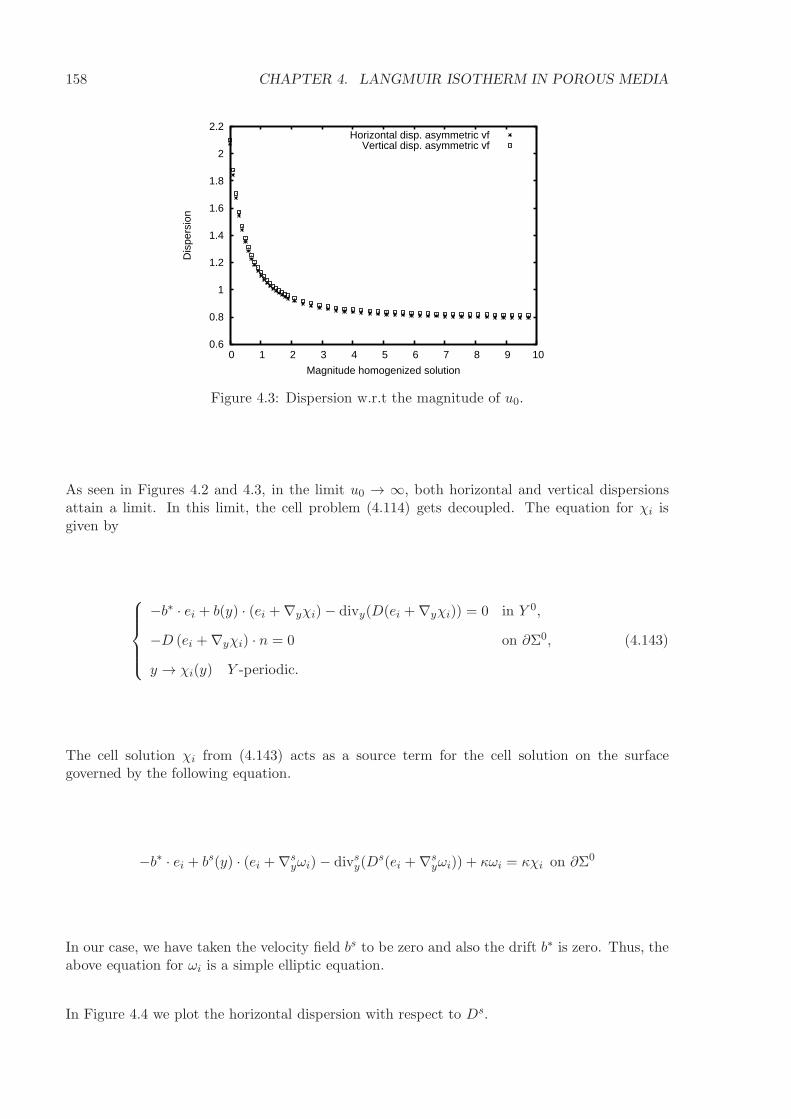
158 CHAPTER 4. LANGMUIR ISOTHERM IN POROUS MEDIA
0.6
0.8
1
1.2
1.4
1.6
1.8
2
2.2
0 1 2 3 4 5 6 7 8 9 10
Dis
pers
ion
Magnitude homogenized solution
Horizontal disp. asymmetric vfVertical disp. asymmetric vf
Figure 4.3: Dispersion w.r.t the magnitude of u0.
As seen in Figures 4.2 and 4.3, in the limit u0 → ∞, both horizontal and vertical dispersionsattain a limit. In this limit, the cell problem (4.114) gets decoupled. The equation for χi isgiven by
−b∗ · ei + b(y) · (ei +∇yχi)− divy(D(ei +∇yχi)) = 0 in Y 0,
−D (ei +∇yχi) · n = 0 on ∂Σ0,
y → χi(y) Y -periodic.
(4.143)
The cell solution χi from (4.143) acts as a source term for the cell solution on the surfacegoverned by the following equation.
−b∗ · ei + bs(y) · (ei +∇syωi)− divsy(D
s(ei +∇syωi)) + κωi = κχi on ∂Σ0
In our case, we have taken the velocity field bs to be zero and also the drift b∗ is zero. Thus, theabove equation for ωi is a simple elliptic equation.
In Figure 4.4 we plot the horizontal dispersion with respect to Ds.

4.10. NUMERICAL STUDY 159
0.778
0.779
0.78
0.781
0.782
0.783
0.784
0.785
0 1 2 3 4 5 6 7 8 9 10
Figure 4.4: Horizontal Dispersion w.r.t surface molecular diffusion.
Clearly the dispersion increases with Ds. However, as shown by Figure 4.4, the dispersionreaches a limit as Ds goes to infinity. This can be explained formally by the fact that, in sucha case, the cell solution satisfies in the limit that (ωi + yi) is constant on the pore surface ∂Σ0.In this limit, the bulk correctors χi satisfy the following limit problem
b(y) · ∇yχi − divy(D(∇yχi + ei)) = (b∗ − b) · ei in Y 0,
−D(∇yχi + ei) · n+ b∗i =ακ
(1 + βu0)2
(χi + yi − |∂Σ0|−1
∫
∂Σ0
(χi + yi)dσ(y)
)on ∂Σ0,
y → χi(y) Y -periodic.
(4.144)
In Figure 4.5 we plot the horizontal dispersion with respect to κ.
0.76
0.78
0.8
0.82
0.84
0.86
0.88
0.9
0 100 200 300 400 500 600 700 800
Figure 4.5: Horizontal Dispersion w.r.t reaction rate.
In the limit κ→ ∞, we get an asymptote for the dispersion, corresponding to a limit cell problem

160 CHAPTER 4. LANGMUIR ISOTHERM IN POROUS MEDIA
where χi = ωi. In this limit, the corresponding system satisfied by the bulk correctors χi is
b(y) · ∇yχi − divy(D(∇yχi + ei)) = (b∗ − b) · ei in Y 0,
−D(∇yχi + ei) · n+ (b∗ − bS) · ei =bS(y) · ∇S
yχi − divSy (DS(∇S
yχi + ei)) on ∂Σ0,
y → χi(y) Y -periodic.
(4.145)
Unlike (4.144), the limit cell problem corresponding to the infinite reaction limit is no longerdependent on the homogenized solution u0.
In the final experiment, we wish to compare the homogenized solution u0(t, x) and the recon-structed solution uε(t, x) in the periodic porous medium of period ε = 0.25 where the recon-structed solution uε(t, x) is given by
uε(t, x) = u0(t, x) + ε(χ1(x/ε)∂x1u0(t, x) + χ2(x/ε)∂x2u0(t, x)
)(4.146)
The solutions to the cell problem (χ1, χ2) are computed in the unit cell. Figure 4.6 depicts thecell solutions χ1 and χ2. Then, they are copied to each cell in the periodic domain where thecells are of size (0.25)2.
IsoValue-0.13506-0.120865-0.106669-0.092474-0.0782787-0.0640833-0.0498879-0.0356925-0.0214971-0.007301670.006893730.02108910.03528450.04947990.06367530.07787070.09206610.1062620.1204570.134652
fonction cellule-1IsoValue-0.134855-0.120656-0.106457-0.092258-0.0780589-0.0638597-0.0496606-0.0354614-0.0212623-0.007063160.007135980.02133510.03553430.04973340.06393250.07813170.09233080.106530.1207290.134928
fonction cellule-2
Figure 4.6: Left: Cell solution χ1 in the unit cell, Right: Cell solution χ2 in the unit cell.
The next task is to compute the homogenized solution to the effective equation (4.112). Wehave taken the initial data, (uin, vin), such that the initial data to the homogenized equationhas a compact support in the periodic domain. The well-prepared initial data that we haveconsidered are
uin = 103 ∗max(0.0, x1 − 0.2) ∗ (−min(0.0, x1 − 0.8)) ∗max(0.0, x2 − 0.2) ∗ (−min(0.0, x2 − 0.8))
and vin = αuin.We employ Rothe’s method where we discretize the time derivative in the effective diffusionequation followed by Newton’s method to solve the resulting elliptic equation. Since we areworking with bounded domain, we need to provide boundary conditions on the exterior boundaryof ]0, 1[×]0, 1[. As working with Dirichlet boundary data may lead to boundary layers, we havetaken periodic boundary conditions. Once we have computed the homogenized solution, we cancalculate the reconstructed solution using (4.146). Figures 4.7, 4.8, 4.9 refer to the evolution ofthe exact solution, homogenized solution and reconstructed solution respectively in the periodicporous domain.

4.10. NUMERICAL STUDY 161
Figure 4.7: Exact Solutions: Left, Time instant 0.001; Middle, Time instant 0.005; Right, Timeinstant 0.01.
Figure 4.8: Homogenized Solutions: Left, Time instant 0.001; Middle, Time instant 0.005; Right,Time instant 0.01.
Figure 4.9: Reconstructed Solutions: Left, Time instant 0.001; Middle, Time instant 0.005;Right, Time instant 0.01.
We remark that there isn’t a very good agreement between the exact solution (Figure 4.7) andwith the reconstructed solution (4.9). We believe it is due to the fact that we have taken theperiodicity to be 0.25 which might be too big to appreciate the homogenization results.

162 CHAPTER 4. LANGMUIR ISOTHERM IN POROUS MEDIA
4.11 Comments
The comments on the locally periodic coefficients in Section 3.14 of Chapter 3 do hold true forthe nonlinear model considered in this chapter.
Constraints on the velocity fields
The presence of the nonlinear term in (4.12)-(4.14) forced us to impose a constraint that thebulk and surface drifts are the same i.e.,
1
|Y 0|
∫
Y 0
b(y) dy =1
|∂Σ0|
∫
∂Σ0
bs(y) dσ(y) = b∗. (4.147)
We are unable to upscale, even formally, the microscopic equations (4.12)-(4.14) unless theconstraint (4.147) holds true. The main reason for imposing this equal drift constraint is theinability of the method of two-scale convergence with drift to handle non constant drifts. Weremarked in Section 4.10 that, in two dimensions, the constraint (4.147) translates as b∗ = 0.Only for d ≥ 3 we can have a non zero drift under the assumption (4.147). This difficulty inhandling, at least purely periodic velocity fields, in presence of nonlinear isotherms emphasizethe need for generalizing the method of two-scale convergence with drift to non constant driftscenarios.
Let us consider the following two-scale asymptotic expansions with drift.
uε(t, x) =∑
i≥0
εiui
(t, x− b∗t
ε,x
ε
). (4.148)
The above ansatz (4.148) can be rewritten in the following manner
uε(t, x) =∑
i≥0
εiui
(t,X(−τ, x), x
ε
)(4.149)
where X(τ, x) with τ = ε−1t is the solution of
dX
dτ= b∗
X(0) = x.
(4.150)
In [87], the following singularly perturbed convection equation is studied.
∂uε∂t
+ a · ∇uε +1
εb · ∇uε = 0. (4.151)
There are no fast oscillating coefficients in (4.151) i.e., a = a(t, x) and b = b(t, x). It is shown in[87] that uε admits the following asymptotic expansion.
uε(t, x) =∑
i≥0
εiui
(t, τ, x
)(4.152)
where ui(t, τ, x) are 2π periodic in τ = ε−1t. The authors of [87] consider
dX
dτ= b(t,X)
X(0) = x.
(4.153)

4.11. COMMENTS 163
An assumption is made on the velocity b such that τ → X(τ ; t, x) is 2π periodic in τ . Denotethe Jacobian matrix of x→ X(τ ; t, x) by ∇X(τ ; t, x). It is proved in [87] that the first term of(4.152) is given by
u0(t, τ, x) = v0(t,X(−τ ; t, x)) (4.154)
where v0 satisfies
∂v0∂t
+ a0 · ∇v0 = 0 in (0, T )× Rd. (4.155)
and u0 satisfies
∂u0∂t
+ a0 · ∇v0 = 0 in (0, T )× Rd. (4.156)
with a0 and a0 given by the following expressions
a0(t, x) =1
2π
2π∫
0
∇X(τ ; t, x)−1a(t,X(τ ; t, x)) dτ, (4.157)
a0(t, x) =1
2π
2π∫
0
α(t, τ, x) dτ, (4.158)
with
α(t, τ, x) = ∇X(τ ; t, x)−1(a(t,X(τ ; t, x)) − ∂X
∂t(τ ; t, x)
). (4.159)
Remark the similarities between (4.149) and (4.154). Once again, it should be noted that theproblem studied in [87] has no fast oscillating coefficients in (4.151). We hope that a carefuladaptation of some of the results from [87] can result in a generalization of the method of two-scale asymptotic with drift by replacing the constant drift b∗ in (4.150) by a variable. Of course,the approach of [87] makes certain assumptions on the velocity field b (please refer to [87] fordetails) in order to guarantee 2π periodic solutions for (4.153). Asymptotic expansions similarto the ones used in [87] had appeared earlier in [123] in the context of Euler equations withrapidly varying initial data.
Conclusions
This Chapter considered the upscaling of reactive flow equations with Langmuir isotherm inperiodic porous media. The lack of technical tools in the theory of homogenization has restrictedthe analysis as can be gathered by the equal drifts assumption (4.147). In Section 3.12 ofChapter 3, we considered compressible flows. We had used Factorization principle to homogenizethe model. The presence of the nonlinear term in the present chapter has restricted us fromrelaxing the incompressibility condition on the velocity fields as is not clear as to the approachof the principle of Factorization adapted to the nonlinear setting. So, there is a lot of roomfor improvement with regard to the homogenization of the current nonlinear adsorption model.Even though we have demonstrated the calculations for the Langmuir isotherm, the result ofhomogenization holds to in case of Freundlich isotherm too. However, the technical details getmore involved in the latter case. In the previous and the current chapters, we studied singlecomponent flows. The next Chapter aims at generalizing the results to the multicomponentflows.

164 CHAPTER 4. LANGMUIR ISOTHERM IN POROUS MEDIA

Chapter 5
Multicomponent flows
5.1 Introduction
Chapters 3 and 4 were dedicated to the study of reactive transport of a single dissolved solute in afluid filling the porous medium, the type of reaction considered being the adsorption/desorptiontype. In Section 3.12 of Chapter 3, we even remarked that the presence of a compressiblefluid is equivalent to the study of convection diffusion reaction equation in the fluid bulk. ThisChapter tries to generalize the results obtained previously to the transport of multiple solutesin porous media. In presence of multiple components, one approach would be to considertransport equations for each of the scalar quantities with no coupling terms. The approachof decoupled system is simple. In the present work, we study a system of convection-diffusionequations coupled through a zero order term. As in all homogenization problems, we scale theadimensionalized system. The scaling considered is parabolic i.e., (τ, y) → (ε−2t, ε−1x). Homog-enization of parabolically scaled scalar parabolic equation with a zero order term was studiedin [76] where they showed the induction of a large drift in the concentration profiles of the ho-mogenized solution. In [25] the results of [76] are adopted in the case of transport phenomenain porous media. In [25], reactions are considered both in the bulk (zero order term) and on thesurface of the porous skeleton (non-homogeneous Neumann boundary condition). This Chaptergeneralizes the results in [76] to a multicomponent flow in porous media. The reaction amongmultiple solutes can be modelled mathematically via a coupling matrix (linear model). In [98], acoupled system of convection-diffusion-reaction systems are considered. The problem addressedin [98] is in a porous medium with semi-permeable porous skeleton using the double-porositymodel [29]. The system they study, however, is under different scaling (Diffusion dominatedregime) which avoids the phenomena of drift in the concentration profiles.
The motivation for the choice of scaling to be parabolic is to study the long term behaviour ofthe system. It is to be noted that there are other scaling techniques available. One such amongthem is the hyperbolic scaling where the space variable is scaled as in the parabolic scalingwhereas the time variable is scaled as τ → ε−1t. In other words, for shorter times. In [139] and[128] hyperbolic scaling is considered in connection to the study of motor proteins.
Starting with a Cauchy problem for a coupled convection-diffusion-reaction system of which uεαare solutions, we show in Proposition 5.4.1 that they admit a representation, for 1 ≤ α ≤ N ,
uεα(t, x) ≈ exp (−λt/ε2)ϕα
(xε
)(v(t, x− b∗
εt)+ ε
d∑
i=1
∂v
∂xi
(t, x− b∗
εt)ωi,α
(xε
))
where (λ, ϕα) is the first eigenpair associated with an eigen cell problem. The drift velocity b∗ is
165

166 CHAPTER 5. MULTICOMPONENT FLOWS
given in term of the microscopic velocity fields, diffusion matrices and the eigenfunctions of thesame eigen cell problem and its adjoint. v is the solution of the following scalar homogenizeddiffusion equation.
ρ∗∂v
∂t− div(D∇v) = 0.
Making the change of functions: v(t, x) = exp (−λt/ε2)v(t, x − b∗
ε t), we remark that v indeedsatisfies the following scalar convection-diffusion-reaction equation.
ρ∗∂v
∂t+ ρ∗
b∗
ε· ∇v − div(D∇v) + ρ∗
λ
ε2v = 0.
Proposition 5.4.1 has close resemblance with the results obtained in [139], [128]. Their approachis to use the classical exponential transformation uεα = exp(−Rα/ε) and to study an averagedHamilton-Jacobi equation satisfied by the common limit R of Rα in the Crandall-Lions viscositysense. The result of the non-stationary problem studied in [128] is that
uεα(t, x) ≈ φα
(xε
)δ(x− b∗t)
where a Dirac mass appears instead of our homogenized solution v. The drift velocity b∗ =∇H(0) with H being the effective Hamiltonian. The absence of the exponential term in theirresults is because 0 happens to be the first eigenvalue of the associated cell eigen problem.Proposition 5.4.1 uses a formal approach to upscale the system. We use two-scale asymptoticexpansions with drift where we assume that uεα has an the asymptotic expansion in ε wherewe insert the large drift b∗/ε only in the macroscopic variable of the coefficients. This formalmethod of two-scale asymptotics with drift has been recalled in Section 2.6 of Chapter 2. Also,we multiply the asymptotic expression with exp (−λt/ε2) to get rid of any exponential growth.This method of Factorization is detailed in Section 2.8 of Chapter 2. This formal method ofobtaining the homogenized equation will be made rigorous in Sections 5.5 and 5.6 where wederive compactness of the solution sequences (uεα)1≤α≤N in the moving coordinates x + b∗
ε t.Then, using the compactness results of Chapter 2, we can pass to the limit in the variationalformulation of the original problem to arrive at the homogenization result. This concept of drifthas been used in the asymptotic analysis literature for some time now. In case of a stationaryelliptic eigenvalue problem, the concept of drift was used in [51], [53] via θ-exponential eigenvalueproblems. This approach via θ-exponential eigenvalue problems has also been applied in thecontext of multigroup neutronic diffusion models of evolution type in [52]. The drift in the nonstationary parabolic equations was used in [76].In Section 5.7, we consider a multicomponent flow model where the zero order coupling termappears as a Neumann condition on the pore boundaries. The homogenization result concerningthis boundary reaction model is given in Section 5.8. Adsorption isotherm that we studiedin Chapter 3 is also incorporated into a multicomponent flow model in Section 5.9 where eachcomponent is allowed to adsorb/desorb on to the porous skeleton followed by a diffusive reactionamong the adsorbed quantities on the boundary.
5.2 Mathematical model
Let us consider N components dissolved in a fluid filling a porous medium. Denote by uα, the
concentration of the αth component. Consider a system of weakly coupled linear convectiondiffusion reaction equations. The weak coupling is in the sense that the coupling is via zeroorder terms.
ρα∂uα∂τ
+ bα · ∇uα − div(Dα∇uα) +N∑
β=1
Παβuβ = 0 in (0, ζ) × Ωf for each 1 ≤ α ≤ N, (5.1)

5.2. MATHEMATICAL MODEL 167
where ρα is the porosity, bα is the fluid velocity, Dα for each 1 ≤ α ≤ N are the diffusion matricesassociated with the solutes and the coupling matrix Π models the possible bulk reactions. Inreality there is only one velocity field, bα = b present in (5.1) as part of a convection term. Asour analysis works for N velocity fields, one for each of the components, we have considered Nvelocity fields (bα)1≤α≤N . To complete (5.1), we have to supplement it with initial and boundarydata. The boundary data we consider is of Neumann type, i.e., zero flux condition on the surfaceof the pores.
Dα∇uα · n = 0 on (0, ζ)× ∂Ωs for each 1 ≤ α ≤ N. (5.2)
We assume that the coefficients in (5.1) are all Y -periodic. The porosity coefficients ρα(y), forevery 1 ≤ α ≤ N , are assumed to be strictly positive. The velocity fields are assumed to beindependent of time and given. We don’t impose any constraint of incompressibility. In thelinear single solute case studied in Chapter 3 we observed, in Section 3.12, that the conditionof incompressibility on the fluid field can be relaxed. However, this wasn’t the case in Chapter4 where a convection diffusion reaction equation was studied with a zero order nonlinear term.Of course, some regularity is required for the fluid velocity and we assume that
bα(y) ∈ L∞(Y 0;Rd). (5.3)
Associated with N solutes, we have N diffusion matrices Dα(y), each of which are assumed tobe in L∞(Y 0), symmetric and uniformly coercive. That is, there exists a positive constant Csuch that, for any ξ ∈ Rd,
Dα(y)ξ · ξ ≥ C|ξ|2 a.e. in Y 0. (5.4)
Now, the assumptions on the constant coupling matrix (Παβ)1≤α,β≤N . For the wellposedness ofthe system (5.1)-(5.2), we make the following assumption on the coupling matrix:
Παβ ≤ 0 for α 6= β, (5.5)
we also assume that the coupling matrix Π is irreducible i.e.,
1, · · · , N 6= B ∪ B′, B ∩ B′ = ∅ such that Παβ = 0 for α ∈ B, β ∈ B′. (5.6)
The hypothesis (5.5)-(5.6) are borrowed from [152], [11], [53] where systems of elliptic andparabolic equations are studied. A matrix satisfying (5.5) is sometimes referred to as “cooper-ative matrix” or “essentially positive matrix”.
In order to study the system (5.1)-(5.2) in an ε-periodic porous medium, we need to scale it onto the underlying microstructure. As the system under consideration is of evolution type, weneed to scale the time variable too. The scaling that we employ shall be “parabolic scaling” inorder to study the long time behavior of the considered transport phenomena. Upon parabolicscaling (τ, y) → (ε−2t, ε−1x), (5.1)-(5.2) yields, for each 1 ≤ α ≤ N ,
ρεα∂uεα∂t
+1
εbεα · ∇uεα − div(Dε
α∇uεα) +1
ε2
N∑
β=1
Παβuεβ = 0 in (0, T ) × Ωε, (5.7)
Dεα∇uεα · n = 0 on (0, T )× ∂Ωε, (5.8)
uεα(0, x) = uinα (x) x ∈ Rd. (5.9)
As usual upon rescaling, the Y -periodic coefficients of the adimensionalized system turn out to be
ε-periodic in the dimensionalized system. So, ρεα(x) = ρα
(xε
), bε(x) = b
(xε
), Dε
α(x) = Dα
(xε
)
are all ε-periodic coefficients.

168 CHAPTER 5. MULTICOMPONENT FLOWS
5.3 Qualitative analysis
The microscopic model (5.7)-(5.9) models the transport of dissolved solutes in presence of con-vection diffusion and reaction. In Section 2.8 of Chapter 2, while recapping the Factorizationprinciple, we illustrated the method via a parabolically scaled scalar convection diffusion reactionequation (2.95). The present model (5.7)-(5.9) is a generalization to the transport of N solutes.The assumption (5.5) on the coefficients Παβ in the zero order term doesn’t help us obtain apriori estimates on (uεα)1≤α≤N . In the absence of a priori estimates, it would be impossible toapply the compactness results from Homogenization theory of Chapter 2. This difficulty withpartial differential equations with large lower order terms has been long recognized [100], [106],[76], [25]. The idea is to pass through spectral cell problems associated with (5.7)-(5.8).
bα(y) · ∇yϕα − divy
(Dα∇yϕα
)+
N∑
β=1
Παβϕβ = λραϕα in Y 0,
Dα∇yϕα · n = 0 on ∂Σ0,
y → ϕα(y) Y − periodic.
(5.10)
In general we have no maximum principles for systems, thus making Krein-Rutman theorem[108] inapplicable. However in [152] it is shown that the first eigenvalue λ for systems similarin structure to (5.10) is positive, real and simple. And the first eigenfunction can be chosenpositive. Let us denote the first eigenpair for (5.10) by (λ, ϕα). The first eigenvalue λ measuresthe balance between convection-diffusion and reaction. The spectral cell problem (5.10) isn’tself-adjoint. The associated adjoint problem is
−divy(bαϕ∗α)− divy
(Dα∇yϕ
∗α
)+
N∑
β=1
Π∗αβϕ
∗β = λραϕ
∗α in Y 0,
Dα∇yϕ∗α · n+ bα(y) · nϕ∗
α = 0 on ∂Σ0,
y → ϕ∗α(y) Y -periodic,
(5.11)
where Π∗ is the transpose of Π. Again by [152] it follows that the first eigenvalue λ for (5.11) isthe same as that for (5.10). And the first eigenfunction for (5.11) can be chosen positive. Theuniqueness of the eigenfunction of (5.11) is up to a chosen normalization. The normalizationthat we consider is the following
N∑
α=1
∫
Y 0
ϕαϕ∗α dy = 1. (5.12)
Let us denote the first eigenpair for (5.11) by (λ, ϕ∗α). As explained in [12, 76, 25] the first
eigenvalue of the spectral cell problem λ governs the time decay of the solution uεα. So, as isdone in the references cited, we perform time renormalization in the spirit of the factorizationprinciple. Also the first eigenfunction ϕα is factored out of uεα. The idea is to make the followingchange of unknowns
vεα(t, x) = exp (λt/ε2)uεα(t, x)
ϕα
(xε
) . (5.13)
With the above change of unknowns, we will be able to overcome the inability we had with thederivation of a priori estimates. Now we state a result that gives the system satisfied by the newunknown (vεα)1≤α≤N .

5.3. QUALITATIVE ANALYSIS 169
Lemma 5.3.1. The system (5.7)-(5.9) is equivalent to
ϕαϕ∗αρ
εα
∂vεα∂t
+1
εbεα ·∇vεα−div
(Dε
α∇vεα)+
1
ε2
N∑
β=1
Παβϕ∗αϕβ(v
εβ − vεα) = 0 in (0, T )×Ωε, (5.14)
Dεα∇vεα · n = 0 on (0, T )× ∂Ωε, (5.15)
vεα(0, x) =uinα (x)
ϕα
(xε
) x ∈ Rd, (5.16)
for each 1 ≤ α ≤ N , where the components of (vεα)1≤α≤N are defined by (5.13). The convective
velocity, bεα(x) = bα
(xε
), in (5.14) is given by
bα(y) = ϕαϕ∗αbα + ϕαDα∇yϕ
∗α − ϕ∗
αDα∇yϕα for every 1 ≤ α ≤ N (5.17)
and the diffusion matrix, Dεα(x) = Dα
(xε
), in (5.14)-(5.15) is given by
Dα(y) = ϕαϕ∗αDα for every 1 ≤ α ≤ N. (5.18)
Proof. We shall plug the expression (5.13) in (5.7)-(5.9) while keeping in mind the followingchain rule formulae
∂uεα∂t
(t, x) =−λε2
exp (−λt/ε2)ϕα
(xε
)vεα(t, x) + exp (−λt/ε2)ϕα
(xε
)∂vεα∂t
(t, x),
∇(uεα(t, x)
)=
1
εexp (−λt/ε2)vεα(t, x)
(∇yϕα
)(xε
)+ exp (−λt/ε2)ϕα
(xε
)∇xv
εα(t, x).
(5.19)Using the spectral cell problem (5.10) and its adjoint (5.11) and identifying the expressions (5.17)and (5.18), the calculations simplify to yield the system of equations (5.14)-(5.16) satisfied by(vεα)1≤α≤N .
Lemma 5.3.2. The divergence of the convective fields bα satisfy
divy bα =N∑
β=1
Π∗αβϕαϕ
∗β −
N∑
β=1
Παβϕ∗αϕβ (5.20)
Proof. Let us take the divergence of the convective fields bα given in (5.17), we arrive at
divy bα = ϕα
(divy(bαϕ
∗α) + divy(Dα∇yϕ
∗α))+ ϕ∗
α
(bα · ∇yϕα − divy(Dα∇yϕα)
)(5.21)
Using information from the spectral cell problem (5.10) and its adjoint (5.11), we have
divy bα = −λϕαϕ∗α +
N∑
β=1
Π∗αβϕαϕ
∗β + λϕαϕ
∗α −
N∑
β=1
Παβϕ∗αϕβ
Thus we arrive at the result (5.20).
From the expression for the divergence derived in (5.20), it follows that
N∑
α=1
divy bα = 0. (5.22)
By the definition (5.17) of bα, it follows that
bα · n = 0 on ∂Σ0. (5.23)

170 CHAPTER 5. MULTICOMPONENT FLOWS
Lemma 5.3.3. Let (vεα) be a weak solution of (5.14)-(5.16). There exists a constant C, inde-pendent of ε, such that
N∑
α=1
∥∥∥vεα∥∥∥L∞((0,T );L2(Ωε))
+
N∑
α=1
∥∥∥∇vεα∥∥∥L2((0,T )×Ωε)
+1
ε
N∑
α=1
N∑
β=1
∥∥∥vεα − vεβ
∥∥∥L2((0,T )×Ωε)
≤ CN∑
α=1
‖vinα ‖L2(Rd)
(5.24)
Proof. To derive the a priori estimates, we shall multiply (5.14) by vεα and add the thus obtainedexpressions followed by integrating over Ωε.
1
2
d
dt
N∑
α=1
∫
Ωε
ϕαϕ∗αρ
εα|vεα|2 dx− 1
2ε
N∑
α=1
∫
Ωε
div(bεα)|vεα|2 dx
+
N∑
α=1
∫
Ωε
Dεα∇vεα · ∇vεα dx+
1
ε2
N∑
α=1
N∑
β=1
∫
Ωε
Παβϕ∗αϕβ(v
εβ − vεα)v
εα = 0 (5.25)
To derive the energy estimate for (5.14)-(5.16), the spectral cell problem (5.10) and its adjoint(5.11) come in handy. Let us consider the bulk equation in (5.10) and multiply it by ϕ∗
α(vεα)
2
followed by integration over the fluid part Y 0.
∫
Y 0
bα·∇yϕαϕ∗α(v
εα)
2 dy−∫
Y 0
divy
(Dα∇yϕα
)ϕ∗α(v
εα)
2 dy+N∑
β=1
∫
Y 0
Παβϕ∗αϕβ(v
εα)
2 dy−∫
Y 0
λραϕαϕ∗α(v
εα)
2 dy
(5.26)
= −∫
Y 0
divy(bαϕ∗α)ϕα(v
εα)
2 dy −∫
Y 0
ϕαϕ∗αbα · ∇y(v
εα)
2 dy +
∫
Y 0
ϕ∗αDα∇yϕα · ∇y(v
εα)
2 dy
+
∫
Y 0
(vεα)2Dα∇yϕα · ∇yϕ
∗α dy +
N∑
β=1
∫
Y 0
Παβϕ∗αϕβ(v
εα)
2 dy −∫
Y 0
λραϕαϕ∗α(v
εα)
2 dy
= −∫
Y 0
divy(bαϕ∗α)ϕα(v
εα)
2 dy −∫
Y 0
ϕαϕ∗αbα · ∇y(v
εα)
2 dy +
∫
Y 0
ϕ∗αDα∇yϕα · ∇y(v
εα)
2 dy
−∫
Y 0
ϕαDα∇yϕ∗α · ∇y(v
εα)
2 dy +
∫
Y 0
ϕαDα∇yϕ∗α · ∇y(v
εα)
2 dy
+
∫
Y 0
(vεα)2Dα∇yϕα · ∇yϕ
∗α dy +
N∑
β=1
∫
Y 0
Παβϕ∗αϕβ(v
εα)
2 dy −∫
Y 0
λραϕαϕ∗α(v
εα)
2 dy
= −∫
Y 0
divy(bαϕ∗α)ϕα(v
εα)
2 dy −∫
Y 0
divy(Dα∇yϕ∗α)ϕα(v
εα)
2 dy −∫
Y 0
λραϕαϕ∗α(v
εα)
2 dy (5.27)
−∫
Y 0
ϕαϕ∗αbα · ∇y(v
εα)
2 dy +
∫
Y 0
ϕ∗αDα∇yϕα · ∇y(v
εα)
2 dy −∫
Y 0
ϕαDα∇yϕ∗α · ∇y(v
εα)
2 dy (5.28)
+
N∑
β=1
∫
Y 0
Παβϕ∗αϕβ(v
εα)
2 dy = 0. (5.29)

5.4. FORMAL ASYMPTOTICS 171
In the above simplified form, we recognize the adjoint cell problem (5.11) in (5.27). We alsorecognize the expression for bα in (5.28). Taking all these contributions into account, (5.27)-(5.28)-(5.29) result in
−N∑
β=1
∫
Y 0
Π∗αβϕ
∗βϕα(v
εα)
2 dσ(y) −∫
Y 0
bα · ∇y(vεα)
2 dy +
N∑
β=1
∫
Y 0
Παβϕ∗αϕβ(v
εα)
2 dσ(y) = 0 (5.30)
Summing (5.30) over α leads to
N∑
α=1
∫
Y 0
divy bα(vεα)
2 dy = 0. (5.31)
Using the above observation (5.31) in the expression (5.25) results in the following energy esti-mate.
1
2
d
dt
N∑
α=1
∫
Ωε
ϕαϕ∗αρ
εα|vεα|2 dx+
N∑
α=1
∫
Ωε
Dεα∇vεα · ∇vεα dx+
1
ε2
N∑
α=1
N∑
β=1
∫
Ωε
Παβϕ∗αϕβ |vεα − vεβ|2 = 0
(5.32)Integrating the energy estimate (5.32) over (0, T ) yields the a priori estimates (5.24).
In the above Lemma 5.3.3, we have derived a priori estimates for the solution sequences of(5.14)-(5.16) obtained upon performing a change of unknowns (5.13). Now we state a resultasserting the well-posedness of the system of equations (5.7)-(5.9).
Proposition 5.3.4. Assume that the initial data uinα belongs to L2(Rd) ∩ L∞(Rd) for every1 ≤ α ≤ N . For any given ε > 0, there exists a unique solution uεα of (5.7)-(5.9) in thefollowing energy space
uεα ∈ L∞((0, T );L2(Ωε)); ∇uεα ∈ L2((0, T ) × Ωε) for every 1 ≤ α ≤ N. (5.33)
Further if the initial data uinα ≥ 0 in Ωε, then the solution uεα(t, x) ≥ 0 in (0, T ) × Ωε.
We avoid the proof of the Proposition 5.3.4. The arguments of the proof are similar to theexistence results and maximum principles proved in [152], [129], [43].
5.4 Formal asymptotics
This section is concerned with finding the effective behaviour of (5.7)-(5.9). We shall be employ-ing a formal method of asymptotic expansions. We consider the following time renormalizedasymptotic ansatz for the solution uεα.
uεα(t, x) = exp (−λt/ε2)∑
i≥0
εiui,α
(t, x− b∗t
ε,x
ε
)for every 1 ≤ α ≤ N. (5.34)
Proposition 5.4.1. If the ansatz for the solution (uεα) of (5.7)-(5.9) given in (5.34) is true,then the solution formally satisfies
uεα(t, x) ≈ exp (−λt/ε2)ϕα
(xε
)(v(t, x− b∗
εt)+ ε
d∑
i=1
∂v
∂xi
(t, x− b∗
εt)ωi,α
(xε
)), (5.35)

172 CHAPTER 5. MULTICOMPONENT FLOWS
with (λ, ϕα) being the first eigenpair associated with (5.10). The components (ωi,α)1≤α≤N , forevery 1 ≤ i ≤ d, satisfy a so called cell problem.
bα(y) ·(∇yωi,α + ei
)− divy
(Dα
(∇yωi,α + ei
))
+N∑
β=1
Παβϕ∗αϕβ
(ωi,β − ωi,α
)= ϕαϕ
∗αραb
∗ · ei in Y 0,
Dα(∇yωi,α + ei) · n = 0 on ∂Σ0,
y → ωi,α Y -periodic,
(5.36)
where the drift velocity b∗ is given by
b∗ =1
ρ∗
N∑
α=1
∫
Y 0
bα(y) dy (5.37)
where ρ∗ is the effective porosity given by
ρ∗ =
N∑
α=1
∫
Y 0
ϕαϕ∗αρα(y) dy (5.38)
with ϕ∗α the first eigenfunction associated with the adjoint spectral cell problem (5.11).
Further, v in (5.35) satisfies the following scalar homogenized equation:
ρ∗∂v
∂t− div(D∇v) = 0 in (0, T ) × Rd,
v(0, x) =N∑
α=1
uinα (x)
∫
Y 0
ϕ∗α(y) dy in Rd.
(5.39)
where D is defined by
Dij =
N∑
α=1
∫
Y 0
Dα
(∇yωi,α + ei
)·(∇yωj,α + ej
)dy
−1
2
N∑
α,β=1
∫
Y 0
ϕ∗αϕβΠαβ
(ωi,α − ωi,β
)(ωj,α − ωj,β
)dy.
(5.40)
In the expression (5.37) for the effective drift, remark the possibility of having a non zero drifteven in the absence of microscopic convective velocity field. This is sometimes referred to as“Reaction induced convection” in the literature. Before we give the proof of Proposition 5.4.1,we shall state and prove some results that fill in the calculations for the formal asymptoticanalysis with the assumed ansatz (5.34).
Lemma 5.4.2. Each of the zero-order terms in the postulated ansatz (5.34), u0,α(t, x, y), can beexpressed as a product of a purely periodic function and a macroscopic function not depending onthe fast variable y. The purely periodic function turns out to be the first eigenfunction associatedwith the spectral cell problem (5.10).

5.4. FORMAL ASYMPTOTICS 173
Proof. Upon plugging (5.34) into (5.7)-(5.9), we identify the system at order ε−2, for each1 ≤ α ≤ N ,
bα(y) · ∇yu0,α − divy
(Dα∇yu0,α
)+
N∑
β=1
Παβu0,β = λραu0,α in Y 0,
Dα∇yu0,α · n = 0 on ∂Σ0,
y → u0,α Y -periodic.
(5.41)
The above system is a spectral problem same as (5.10) of which λ is the first eigenvalue and ϕα
is the first positive eigenfunction. Thus, we deduce that there exists a function v independentof y such that
u0,α(t, x, y) = ϕα(y)v(t, x) for every 1 ≤ α ≤ N. (5.42)
Lemma 5.4.3. The first order correctors in the postulated ansatz (5.34), u1,α(t, x, y), can bedecomposed as a product of the derivatives of the zero order term and periodic functions satisfyinga system of stationary convection-diffusion-reaction equations in a unit cell which we call thecell problem.
bα(y) ·(∇yωi,α + ei
)− divy
(Dα
(∇yωi,α + ei
))
+N∑
β=1
Παβϕ∗αϕβ
(ωi,β − ωi,α
)= ϕαϕ
∗αραb
∗ · ei in Y 0,
Dα(∇yωi,α + ei) · n = 0 on ∂Σ0,
y → ωi,α Y -periodic,
(5.43)
for every 1 ≤ i ≤ d and for every 1 ≤ α ≤ N . The unknown drift velocity b∗ in the ansatz (5.34)is given by (5.37).
Proof. As with the analysis of asymptotic analysis, we identify the coefficients at different ordersof ε upon substituting (5.34) in (5.7)-(5.9). In the proof of Lemma 5.4.2, we identified the systemat order ε−2. In the current proof, we shall identify the system that we obtain at order ε−1.
bα · ∇yu1,α − divy
(Dα∇yu1,α
)+
N∑
α=1
Παβu1,β − λραu1,α
=(ραb
∗ − bα
)· ∇xu0,α + divy
(Dα∇xu0,α
)+ divx
(Dα∇yu0,α
)in Y 0,
Dα(∇yu1,α +∇xu0,α) · n = 0 on ∂Σ0,
y → u1,α Y -periodic.
(5.44)
Since we know the form of u0,α from (5.42), the linearity of (5.44) help us deduce that
u1,α(t, x, y) =d∑
i=1
∂v
∂xi(t, x)ϕα(y)ωi,α(y) for every 1 ≤ α ≤ N. (5.45)
By taking ϕα(y)ωi,α(y) = ζi,α(y), for every 1 ≤ α ≤ N , we shall write the following system for

174 CHAPTER 5. MULTICOMPONENT FLOWS
(ζi,α)1≤i≤d:
bα(y) · ∇yζi,α − divy
(Dα∇yζi,α
)+
N∑
β=1
Παβζi,β − λραζi,α
= ϕα
(ραb
∗ − bα
)· ei + divy
(ϕαDαei
)+Dα∇yϕα · ei in Y 0,
Dα(∇yζi,α + ϕαei) · n = 0 on ∂Σ0,
y → ζi,α Y -periodic.
(5.46)
Invoking Fredholm alternative we know that the compatibility condition for the existence of firsteigenpair for the above system is that the right hand side of (5.46) is orthogonal to (ϕ∗
α)1≤α≤N ,i.e.,
N∑
α=1
( ∫
Y 0
ϕ∗αϕα
(ραb
∗ − bα
)· ei dy +
∫
Y 0
divy
(ϕαDαei
)ϕ∗α dy
+
∫
Y 0
ϕ∗αDα∇yϕα · ei dy −
∫
∂Σ0
ϕ∗αϕαDαei · n dσ(y)
)= 0
which is nothing but
N∑
α=1
( ∫
Y 0
ϕ∗αϕα
(ραb
∗ − bα
)· ei dy +
∫
Y 0
divy
(ϕαϕ
∗αDαei
)dy −
∫
Y 0
ϕαDα∇yϕ∗α · ei dy
+
∫
Y 0
ϕ∗αDα∇yϕα · ei dy −
∫
∂Σ0
ϕ∗αϕαDαei · n dσ(y)
)= 0
Using the divergence theorem and identifying the expression for bα from (5.17), we have
b∗ =1
ρ∗
N∑
α=1
∫
Y 0
bα(y) dy.
Thus the expression for the drift velocity coincides with (5.37). Now to derive the cell problem(5.43), we shall substitute for (ζi,α) in (5.46) in terms of the eigenfunction (ϕα) and the cellsolutions (ωi,α).
ϕαbα · ∇yωi,α − divy
(ϕαDα∇yωi,α
)−Dα∇yϕα · ∇yωi,α +
N∑
β=1
Παβϕβ
(ωi,β − ωi,α
)
= ϕα
(ραb
∗ − bα
)· ei + divy
(ϕαDαei
)+Dα∇yϕα · ei in Y 0
ϕαDα
(∇yωi,α + ei
)· n = 0 on ∂Σ0,
y → ωi,α Y -periodic.(5.47)
The simplifications to arrive at (5.47) are possible because of the spectral problem (5.10). Now,let us multiply (5.47) by (ϕ∗
α) both in the fluid and on the solid part. A little algebra will thusyield (5.43).

5.4. FORMAL ASYMPTOTICS 175
Before we proceed with the proof of Proposition 5.4.1 let us consider the variational formulationfor the cell problem (5.36) with (φα)1≤α≤N as test functions.
N∑
α=1
∫
Y 0
(bα · ∇yωi,α
)φα dy +
N∑
α=1
∫
Y 0
Dα
(∇yωi,α + ei
)· ∇yφα dy
+
N∑
α=1
N∑
β=1
∫
Y 0
Παβϕ∗αϕβ
(ωi,β − ωi,α
)φα dy =
N∑
α=1
∫
Y 0
(ϕαϕ
∗αραb
∗ − bα
)· eiφα dy. (5.48)
Proof of Proposition 5.4.1. From Lemma 5.4.2 we have found the structure (5.42) of the zeroorder term in (5.34) and from Lemma 5.4.3 we have the structure of the cell problem (5.43).Continuing the identification of the coefficients, the system corresponding to the coefficients ofε0 among the cascade is
bα · ∇yu2,α − divy
(Dα∇yu2,α
)+
N∑
β=1
Παβu2,β − λραu2,α = −ρα∂u0,α∂t
+(ραb
∗ − bα
)· ∇xu1,α + divx
(Dα
(∇xu0,α +∇yu1,α
))+ divy
(Dα∇xu1,α
)in Y 0,
Dα
(∇yu2,α +∇xu1,α
)· n = 0 on ∂Σ0,
y → u2,α Y -periodic.(5.49)
The solvability of the above eigenvalue problem follows from the Fredholm alternative. Thecompatibility condition being that the right hand side of (5.44) is orthogonal to (ϕ∗
α)1≤α≤N . Weshall compute term by term.
−N∑
α=1
∫
Y 0
ραϕ∗α
∂u0,α∂t
dy = −∂v∂t
N∑
α=1
∫
Y 0
ϕαϕ∗αρα dy = −ρ∗∂v
∂t, (5.50)
N∑
α=1
∫
Y 0
ϕ∗α(ραb
∗ − bα) · ∇xu1,α dy =∂
∂xi
N∑
α=1
∫
Y 0
ϕαϕ∗αωj,α(ραb
∗ − bα) · ei dy ∂v
∂xj, (5.51)
N∑
α=1
divx
∫
Y 0
ϕ∗αDα∇xu0,α dy =
∂
∂xi
N∑
α=1
∫
Y 0
Dαej · ei dy ∂v∂xj
, (5.52)
N∑
α=1
divx
∫
Y 0
ϕ∗αDα∇yu1,α dy =
∂
∂xi
N∑
α=1
∫
Y 0
Dα∇yωj,α · ei dy ∂v
∂xj
+∂
∂xi
N∑
α=1
∫
Y 0
(ωj,αϕ∗αDα∇yϕα · ei dy
∂v∂xj
, (5.53)
N∑
α=1
∫
Y 0
divy(Dα∇xu1,α)ϕ∗α dy = −
N∑
α=1
∫
Y 0
Dα∇xu1,α · ∇yϕ∗α dy +
N∑
α=1
∫
∂Σ0
ϕ∗αDα∇xu1,α · n dσ(y)

176 CHAPTER 5. MULTICOMPONENT FLOWS
= − ∂
∂xi
N∑
α=1
∫
Y 0
ωj,αϕαDα∇yϕ∗α · ei dy
∂v∂xj
. (5.54)
The boundary integrals disappear in (5.54) as they cancel off with the terms due to the Neumanncondition in (5.49). Adding the terms (5.50) through (5.54), we arrive at an equation of theform
ρ∗∂v
∂t− div(D∇v) = 0 (5.55)
with the elements of D given by
Dij =
N∑
α=1
∫
Y 0
Dαej · ei dy +1
2
N∑
α=1
∫
Y 0
(Dα∇yωi,α · ej + Dα∇yωj,α · ei
)dy
+1
2
N∑
α=1
∫
Y 0
(ωi,α(ϕαϕ
∗αραb
∗ − bα) · ej + ωj,α(ϕαϕ∗αραb
∗ − bα) · ei)dy
(5.56)
In the expression (5.56) for D, the dispersion tensor is symmetrized. The observation (2.51) thatwe made in Chapter 2 implies that the non symmetric part of the dispersion matrix D doesn’tcontribute to the homogenized equation (5.55) as the Hessian matrix ∇∇v is symmetric. Theexpression (5.56) for D is given in terms of the cell solutions (ωi,α)1≤i≤d;1≤α≤N . To obtainthe expression for the elements of D given in (5.40), we shall use information from the cellproblem (5.36). Let us consider the variational formulation (5.48) for (ωi,α) in (5.36) withtest function (φα)1≤α≤N = (ωj,α)1≤α≤N . Then the one for (ωj,α) in (5.36) with test function(φα)1≤α≤N = (ωi,α)1≤α≤N . This leads to
1
2
N∑
α=1
∫
Y 0
(ωi,α(ϕαϕ
∗αραb
∗ − bα) · ej + ωj,α(ϕαϕ∗αραb
∗ − bα) · ei)dy
=
N∑
α=1
∫
Y 0
Dα∇yωi,α · ∇yωj,α dy +1
2
N∑
α=1
∫
Y 0
(Dα∇yωi,α · ej + Dα∇yωj,α · ei
)dy
−1
2
N∑
α=1
∫
Y 0
ωi,αωj,αdivy bα dy
+1
2
N∑
α=1
N∑
β=1
∫
Y 0
(Παβϕ
∗αϕβ(ωi,β − ωi,α)ωj,α +Παβϕ
∗αϕβ(ωj,β − ωj,α)ωi,α
)dy. (5.57)
Lemma 5.3.2 gives an expression for the divergence of the convective field bα in (5.20) whichwill lead us to conclude that the right hand side of (5.57) is same as
N∑
α=1
∫
Y 0
Dα∇yωi,α · ∇yωj,α dy +1
2
N∑
α=1
∫
Y 0
(Dα∇yωi,α · ej + Dα∇yωj,α · ei
)dy
−1
2
N∑
α=1
N∑
β=1
∫
Y 0
ϕ∗αϕβΠαβ
(ωi,α − ωi,β
)(ωj,α − ωj,β
)dy (5.58)

5.5. TWO-SCALE COMPACTNESS 177
Using information from (5.57) and (5.58) in the expression for D in (5.56) leads to a compactexpression for the dispersion matrix.
Dij =
N∑
α=1
∫
Y 0
Dα
(∇yωi,α + ei
)·(∇yωj,α + ej
)dy
−1
2
N∑
α=1
N∑
β=1
∫
Y 0
ϕ∗αϕβΠαβ
(ωi,α − ωi,β
)(ωj,α − ωj,β
)dy
Lemma 5.4.4. The dispersion matrix D given by (5.40) is symmetric positive definite.
Proof. The symmetric part is obvious because of the way we derived the expression for D. By thehypothesis on the coupling matrix and the positivity of the first eigenvector functions, the factorΠαβϕ
∗αϕβ is always negative. We have also chosen the diffusion matrices Dα to be coercive. For
ξ ∈ Rd, we shall define
ωαξ =d∑
i=1
ωi,αξi
Then,
Dξ · ξ ≥N∑
α=1
cα
∫
Y 0
∣∣∣∇yωαξ + ξ∣∣∣2dy +
N∑
α=1
N∑
β=1
cαβ
∫
Y 0
∣∣∣ωαξ − ωβξ
∣∣∣2dy ≥ 0.
Now, we need to show that Dξ · ξ > 0 for all ξ 6= 0. Suppose that Dξ · ξ = 0 which in turnimplies that
ωαξ + ξ · y ≡ Cα, ωαξ − ωβξ ≡ Cαβ
for some constants Cα, Cαβ . As the cell solutions (ωi,α) are Y−periodic, it cannot be affine.Thus the above equalities are possible only when ξ = 0. Thus implying the positive definitenessof D.
5.5 Two-scale compactness
This section is devoted to finding two-scale limits with drift for the sequence of solutions for themicroscopic model (5.7)-(5.9). We prove a theorem which is in the same spirit as Theorem 3.8.2of Chapter 3 and Theorem 4.7.2 of Chapter 4. As before, the a priori estimates on the solutionscome in handy.
Theorem 5.5.1. Let b∗ ∈ Rd be given by (5.37). There exists v ∈ L2((0, T );H1(Rd)) and(v1,α) ∈ L2((0, T ) × Rd;H1(Y 0)), for each 1 ≤ α ≤ N , such that the sequence of concentrations(vεα)1≤α≤N ∈ L2((0, T );H1(Ωε))
N , solutions of system (5.14)-(5.16), two-scale converge withdrift b∗, up to a subsequence, as ε→ 0, in the following sense
vεα2−drift−−−− v, ∇vεα
2−drift−−−− ∇xv +∇yv1,α,1
ε
(vεα − vεβ
)2−drift−−−− v1,α − v1,β,
(5.59)for every 1 ≤ α, β ≤ N .

178 CHAPTER 5. MULTICOMPONENT FLOWS
Proof. Consider the a priori bounds (5.24) on vεα obtained in Lemma 5.3.3. It follows fromProposition 2.6.4 of Chapter 2 that there exist two-scale limits, say vα ∈ L2(0, T ;L2(Rd)) suchthat
vεα2−drift−−−− vα (5.60)
for every 1 ≤ α ≤ N . Also from the a priori estimates (5.24) we have
N∑
α=1
N∑
β=1
T∫
0
∫
Ωε
(vεα − vεβ
)2dx dt ≤ Cε2. (5.61)
The estimate (5.61) implies that the limits obtained in (5.60) do match i.e., vα = v for every1 ≤ α ≤ N . The H1 a priori estimate in space as in (5.24) does imply that v ∈ L2(0, T ;H1(Rd))and that there exist limits v1,α ∈ L2(0, T ×Rd;H1(Y 0)) such that
∇vεα2−drift−−−− ∇xv +∇yv1,α (5.62)
for every 1 ≤ α ≤ N . However, the limit of the coupled term isn’t straightforward. Since1
ε(vεα−vεβ) is bounded in L2((0, T )×Ωε), we have the existence of q(t, x, y) ∈ L2((0, T )×Rd×Y 0)
such that
limε→0
T∫
0
∫
Ωε
1
ε(vεα − vεβ)φ
(t, x− b∗
εt,x
ε
)dx dt =
T∫
0
∫
Rd
∫
Y 0
q(t, x, y)φ(t, x, y) dy dx dt (5.63)
Taking Ψ ∈ L2((0, T ) × Rd × Y 0)d, let us consider
T∫
0
∫
Ωε
(∇vεα −∇vεβ
)·Ψ(t, x− b∗
εt,x
ε
)dx dt =
−T∫
0
∫
Ωε
(vεα−vεβ
)divxΨ
(t, x− b∗
εt,x
ε
)dx dt−
T∫
0
∫
Ωε
1
ε
(vεα−vεβ
)divyΨ
(t, x− b∗
εt,x
ε
)dx dt (5.64)
Upon passing to the limit in (5.64) as ε→ 0, the first term on the right hand side vanishes as thelimits of vεα and vεβ match and the second term on the right hand side as in (5.63). Consideringthe limit (5.62), upon passing to the limit as ε→ 0 in (5.64) we have
T∫
0
∫
Rd
∫
Y 0
∇y
(v1,α − v1,β
)·Ψ(t, x, y) dy dx dt = −
T∫
0
∫
Rd
∫
Y 0
q(t, x, y)divyΨ(t, x, y) dy dx dt (5.65)
From (5.65) we deduce that (v1,α − v1,β) and q(t, x, y) differ by a function of (t, x), say l(t, x).As v1,α and v1,β are also defined up to the addition of a function solely dependent on (t, x), wecan get rid of l(t, x) and we recover indeed the following limit
1
ε
(vεα − vεβ
)2−drift−−−− v1,α − v1,β.

5.6. PROOF OF HOMOGENIZATION RESULT 179
5.6 Proof of homogenization result
This section is dedicated to the rigorous justification of the formal result, Proposition 5.4.1, thatwe have obtained in Section 5.4. The following theorem characterizes the two-scale limits foundin Theorem 5.5.1.
Theorem 5.6.1. Let v ∈ L2((0, T );H1(Rd)) and v1,α ∈ L2((0, T ) × Rd;H1(Y 0)) for every 1 ≤α ≤ N be the limits obtained in (5.59). The two-scale limits v1,α admit an explicit representationgiven by
v1,α(t, x, y) =d∑
i=1
∂v
∂xi(t, x)ωi,α(y) for every 1 ≤ α ≤ N (5.66)
where (ωi,α)1≤i≤d satisfy the cell problem (5.36). Further, the two-scale limit v(t, x) is the uniquesolution of the homogenized problem (5.39) with the elements of the dispersion matrix D givenby (5.40).
Proof. The idea is to test the bulk equation (5.14) in the factorized system (5.14)-(5.16) with
φεα = φ
(t, x− b∗t
ε
)+ εφ1,α
(t, x− b∗t
ε,x
ε
). (5.67)
Here φ(t, x) and φ1,α(t, x, y) are smooth compactly supported functions which vanish at the finaltime T .
N∑
α=1
T∫
0
∫
Ωε
ϕαϕ∗αρ
εα
∂vεα∂t
φεα dx dt+1
ε
N∑
α=1
T∫
0
∫
Ωε
bεα · ∇vεαφεα dx dt+N∑
α=1
T∫
0
∫
Ωε
Dεα∇vεα · ∇φεα dx dt
+1
ε2
N∑
α=1
N∑
β=1
T∫
0
∫
Ωε
Παβϕ∗αϕβ(v
εβ − vεα)φ
εα = 0. (5.68)
Substituting for φεα from (5.67) in the variational formulation (5.68) and integrating by partslead to
−N∑
α=1
T∫
0
∫
Ωε
ϕαϕ∗αρ
εαv
εα
∂φ
∂t
(t, x− b∗
εt)dx dt+
1
ε
N∑
α=1
T∫
0
∫
Ωε
ϕαϕ∗αρ
εαv
εαb
∗ · ∇xφ(t, x− b∗
εt)dx dt
−1
ε
N∑
α=1
T∫
0
∫
Ωε
div(bεα
)vεαφ
(t, x− b∗
εt)dx dt− 1
ε
N∑
α=1
T∫
0
∫
Ωε
vεαbεα · ∇xφ
(t, x− b∗
εt)dx dt
+
N∑
α=1
T∫
0
∫
Ωε
Dεα∇vεα ·∇xφ
(t, x− b∗
εt)dx dt+
1
ε2
N∑
α=1
N∑
β=1
T∫
0
∫
Ωε
Παβϕ∗αϕβ(v
εβ−vεα)φ
(t, x− b∗
εt)dx dt
+N∑
α=1
T∫
0
∫
Ωε
ϕαϕ∗αρ
εαv
εαb
∗ ·∇φ1,α(t, x− b∗
εt,x
ε
)dx dt+
N∑
α=1
T∫
0
∫
Ωε
(bεα ·∇vεα
)φ1,α
(t, x− b∗
εt,x
ε
)dx dt
+
N∑
α=1
T∫
0
∫
Ωε
Dεα∇vεα · ∇yφ1,α
(t, x− b∗
εt,x
ε
)dx dt

180 CHAPTER 5. MULTICOMPONENT FLOWS
+1
ε
N∑
α=1
N∑
β=1
T∫
0
∫
Ωε
Παβϕ∗αϕβ(v
εβ − vεα)φ1,α
(t, x− b∗
εt,x
ε
)dx dt+O(ε) = 0. (5.69)
Taking φ ≡ 0 in (5.69), we arrive at a variational formulation involving only φ1,α.
N∑
α=1
T∫
0
∫
Ωε
ϕαϕ∗αv
εαρ
εαb
∗ ·∇φ1,α(t, x− b∗
εt,x
ε
)dx dt+
N∑
α=1
T∫
0
∫
Ωε
(bεα ·∇vεα
)φ1,α
(t, x− b∗
εt,x
ε
)dx dt
+
N∑
α=1
T∫
0
∫
Ωε
Dεα∇vεα · ∇yφ1,α
(t, x− b∗
εt,x
ε
)dx dt
+1
ε
N∑
α=1
N∑
β=1
T∫
0
∫
Ωε
Παβϕ∗αϕβ(v
εβ − vεα)φ1,α
(t, x− b∗
εt,x
ε
)dx dt = 0. (5.70)
Passing to the limit in (5.70) as ε→ 0 yields
−N∑
α=1
T∫
0
∫
Rd
∫
Y 0
ϕαϕ∗αραb
∗ · ∇xv(t, x)φ1,α(t, x, y) dy dx dt
+
N∑
α=1
T∫
0
∫
Rd
∫
Y 0
bα ·(∇xv(t, x) +∇yv1,α(t, x, y)
)φ1,α(t, x, y) dy dx dt
−N∑
α=1
T∫
0
∫
Rd
∫
Y 0
divy
(Dα
(∇xv(t, x) +∇yv1,α(t, x, y)
))φ1,α(t, x, y) dy dx dt
+
N∑
α=1
N∑
β=1
T∫
0
∫
Rd
∫
Y 0
Παβϕ∗αϕβ
(v1,β(t, x, y)− v1,α(t, x, y)
)φ1,α(t, x, y) dy dx dt = 0. (5.71)
The above expression (5.71) is the variational formulation for
bα ·(∇yv1,α +∇xv
)− divy
(Dα
(∇yv1,α +∇xv
))
+N∑
β=1
Παβϕ∗αϕβ(v1,β − v1,α) = ϕαϕ
∗αραb
∗ · ∇xv in Y 0,
Dα
(∇yv1,α +∇xv
)· n = 0 on ∂Σ0,
y → v1,α Y -periodic.
(5.72)
for every 1 ≤ α ≤ N . By Fredholm alternative we have the existence and uniqueness ofv1,α ∈ L2(0, T ×Rd;H1(Y 0)/R) if and only if the drift velocity b∗ satisfies (5.37) which is indeedthe value we chose for the drift velocity in Theorem 5.5.1. Also by linearity of (5.72), we deducethat we can separate the slow and fast variables in v1,α as in (5.66) with ωi,α satisfying thecoupled cell problem (5.36).

5.6. PROOF OF HOMOGENIZATION RESULT 181
As a next step, we shall choose φ1,α ≡ (0, 0) in the variational expression (5.69). This gives usa variational formulation involving only φ.
−N∑
α=1
T∫
0
∫
Ωε
ϕαϕ∗αρ
εαv
εα
∂φ
∂t
(t, x− b∗
εt)dx dt+
1
ε
N∑
α=1
T∫
0
∫
Ωε
ϕαϕ∗αv
εαρ
εαb
∗ · ∇xφ(t, x− b∗
εt)dx dt
−1
ε
N∑
α=1
T∫
0
∫
Ωε
div(bεα
)vεαφ
(t, x− b∗
εt)dx dt− 1
ε
N∑
α=1
T∫
0
∫
Ωε
vεαbεα · ∇xφ
(t, x− b∗
εt)dx dt
+
N∑
α=1
T∫
0
∫
Ωε
Dεα∇vεα·∇xφ
(t, x−b
∗
εt)dx dt+
1
ε2
N∑
α=1
N∑
β=1
T∫
0
∫
Ωε
Παβϕ∗αϕβ(v
εβ−vεα)φ
(t, x−b
∗
εt)dx dt = 0.
(5.73)Thanks to the expressions for the divergence of bα in (5.20) as they help us get rid of the termsof order ε−2 in the variational formulation (5.73). There are still some problematic terms oforder ε−1 in the variational formulation (5.73). To simplify them we shall introduce an auxiliaryproblem which is well-posed, thanks to the expression for the drift velocity b∗ from (5.37).
−∆Ξ =
N∑
α=1
ϕαϕ∗αραb
∗ − bα in Y 0,
−∇Ξ · n = 0 on ∂Σ0,
y → Ξ(y) is Y -periodic.
(5.74)
The scaled auxiliary problem associated with (5.74) shall be
−ε2∆Ξε(x/ε) =
N∑
α=1
ϕαϕ∗αρ
εαb
∗ − bεα in Ωε,
−ε∇Ξε(x/ε) · n = 0 on ∂Ωε,
x→ Ξε is ε− periodic.
(5.75)
Now, let us regroup the problematic terms from (5.73) as we are equipped to handle them.
1
ε
N∑
α=1
T∫
0
∫
Ωε
ϕαϕ∗αρ
εαv
εαb
∗ · ∇xφ(t, x− b∗
εt)dx dt− 1
ε
N∑
α=1
T∫
0
∫
Ωε
vεαbεα · ∇xφ
(t, x− b∗
εt)dx dt
= −ε2
ε
T∫
0
∫
Ωε
∆Ξεi
∂φ
∂xivεα dx dt+
1
ε
N∑
β=1
T∫
0
∫
Ωε
ϕβϕ∗βρ
εβ(v
εβ − vεα)b
∗ · ∇xφdx dt
+1
ε
N∑
β=1
T∫
0
∫
Ωε
(vεα − vεβ)bεβ · ∇xφ
(t, x− b∗
εt)dx dt
= ε
T∫
0
∫
Ωε
∇Ξεi · ∇
( ∂φ∂xi
)vεα dx dt+ ε
T∫
0
∫
Ωε
∇Ξεi · ∇vεα
( ∂φ∂xi
)dx dt

182 CHAPTER 5. MULTICOMPONENT FLOWS
+1
ε
N∑
β=1
T∫
0
∫
Ωε
ϕβϕ∗βρ
εβ(v
εβ−vεα)b∗ ·∇xφdx dt+
1
ε
N∑
β=1
T∫
0
∫
Ωε
(vεα−vεβ)bεβ ·∇xφ(t, x− b∗
εt)dx dt (5.76)
Using (5.76) in (5.73) we write down the final variational formulation where we can pass to thelimit as we know the two-scale limits of all the sequences involved.
−N∑
α=1
T∫
0
∫
Ωε
ϕαϕ∗αρ
εαv
εα
∂φ
∂t
(t, x− b∗
εt)dx dt+
N∑
α=1
T∫
0
∫
Ωε
Dεα∇vεα · ∇xφ
(t, x− b∗
εt)dx dt
+ε
T∫
0
∫
Ωε
∇Ξεi · ∇
( ∂φ∂xi
)vεα dx dt+ ε
T∫
0
∫
Ωε
∇Ξεi · ∇vεα
( ∂φ∂xi
)dx dt
+1
ε
N∑
β=1
T∫
0
∫
Ωε
ϕβϕ∗βρ
εβ(v
εβ − vεα)b∗ ·∇xφdx dt+
1
ε
N∑
β=1
T∫
0
∫
Ωε
(vεα − vεβ)bεβ ·∇xφ(t, x− b∗
εt)dx dt = 0.
(5.77)Passing to the limit as ε→ 0 in (5.77) we have
T∫
0
∫
Rd
ρ∗∂v
∂tφ dx dt+
T∫
0
∫
Rd
∫
Y 0
∇yΞi ·∇yv1,α∂φ
∂xidy dx dt+
N∑
α=1
T∫
0
∫
Rd
∫
Y 0
Dα
(∇v+∇yv1,α
)·∇xφdx dt
+
N∑
β=1
T∫
0
∫
Rd
∫
Y 0
ϕβϕ∗βρβ
(v1,β−v1,α
)b∗ ·∇xφdy dx dt+
N∑
β=1
T∫
0
∫
Rd
∫
Y 0
(v1,α−v1,β
)bβ ·∇xφdy dx dt = 0.
(5.78)We know the representations for v1,α from (5.66) in terms of the cell solutions. We shall substi-tute them in the limit equation (5.78).
T∫
0
∫
Rd
∂v
∂tφ dx dt−
∑
i,j
T∫
0
∫
Rd
∂v
∂xj
∂φ
∂xi
∫
Y 0
(∆yΞi
)ωj,α dy dx dt
+N∑
α=1
∑
i,j
T∫
0
∫
Rd
∂v
∂xj
∂φ
∂xi
∫
Y 0
Dα
(∇yj +∇yωj,α
)· ∇yi dy dx dt
+
N∑
β=1
∑
i,j
T∫
0
∫
Rd
∂v
∂xj
∂φ
∂xi
∫
Y 0
ϕβϕ∗βρβ
(ωj,β − ωj,α
)b∗ · ∇yi dy dx dt
+N∑
β=1
∑
i,j
T∫
0
∫
Rd
∂v
∂xj
∂φ
∂xi
∫
Y 0
(ωj,α − ωj,β
)bβ · ∇yi dy dx dt = 0. (5.79)
The expression (5.79) is a variational formulation of the homogenized equation (5.39). Usingthe auxiliary problem (5.74) we shall give the elements of D
Dij =
N∑
α=1
∫
Y 0
Dα
(∇yj+∇yωj,α
)·∇yi dy+
N∑
α=1
∫
Y 0
ϕαϕ∗αραωj,αb
∗ ·ei dy−N∑
α=1
∫
Y 0
ωj,αbα ·ei dy. (5.80)

5.7. BOUNDARY REACTION: MODEL AND QUALITATIVE ANALYSIS 183
The non symmetric part of D doesn’t play the role in the homogenized equation (5.39) asexplained in Section 5.4. The dispersion matrix D in (5.80) upon symmetrizing leads to
Dij =
N∑
α=1
∫
Y 0
Dαej · ei dy +1
2
N∑
α=1
∫
Y 0
(Dα∇yωi,α · ej + Dα∇yωj,α · ei
)dy
+1
2
N∑
α=1
∫
Y 0
(ωi,α(ϕαϕ
∗αραb
∗ − bα) · ej + ωj,α(ϕαϕ∗αραb
∗ − bα) · ei)dy. (5.81)
The symmetric expression in (5.81) is the same as the one obtained in (5.56) via the formalmethod in Section 5.4. We can redo the calculations that followed (5.56) using the cell problem(5.36) to arrive at
Dij =N∑
α=1
∫
Y 0
Dα
(∇yωi,α + ei
)·(∇yωj,α + ej
)dy
−1
2
N∑
α=1
N∑
β=1
∫
Y 0
ϕ∗αϕβΠαβ
(ωi,α − ωi,β
)(ωj,α − ωj,β
)dy.
Remark 5.6.2. The irreducibility assumption (5.6) on the coupling matrix Π ensures micro-scopic equilibrium among solutes resulting in a single homogenized concentration v(t, x) i.e., ifthe coupling matrix Π ≡ 0 (say), we get N different homogenized concentrations.
5.7 Boundary reaction: Model and qualitative analysis
In this Chapter, so far we have studied a system of convection diffusion reaction equations(5.7)-(5.9) where the bulk reactions are considered and the reaction terms appear as a zeroorder term in (5.7). Now, we shall slightly modify the reaction model. Let us consider surfacereaction terms, similar to the bulk reaction term in (5.7). This model is very close to (5.7)-(5.9)except for the reactions on the boundary and absence of bulk reactions, for each 1 ≤ α ≤ N ,
ρα∂uα∂τ
+ bα(y) · ∇uα − div(Dα∇uα) = 0 in (0, ζ)× Ωf , (5.82)
−Dα∇uα · n =N∑
β=1
Παβuβ on (0, ζ)× Ωs. (5.83)
We will be working with the same hypothesis on all the coefficients as before. Upon parabolicscaling, (5.82)-(5.83) yields
ρεα∂uεα∂t
+1
εbεα · ∇uεα − div(Dε
α∇uεα) = 0 in (0, T ) × Ωε, (5.84)
−Dεα∇uεα · n =
1
ε
N∑
β=1
Παβuεβ on (0, T ) × ∂Ωε, (5.85)
uεα(0, x) = uinα (x) x ∈ Rd. (5.86)
In Section 5.3 we remarked that the difficulty in arriving at the a priori estimates for (5.7)-(5.9)could be overcome by spectral cell problems associated with (5.7)-(5.9) followed by a factorization

184 CHAPTER 5. MULTICOMPONENT FLOWS
principle. We shall employ the same approach to treat the current model too. Let us considerthe spectral and its adjoint cell problems, for each 1 ≤ α ≤ N ,
bα(y) · ∇yϕα − divy
(Dα∇yϕα
)= λραϕα in Y 0,
−Dα∇yϕα · n =
N∑
β=1
Παβϕβ on ∂Σ0,
y → ϕα(y) Y -periodic.
(5.87)
−divy(bαϕ∗α)− divy
(Dα∇yϕ
∗α
)= λραϕ
∗α in Y 0,
−Dα∇yϕ∗α · n− bα(y) · nϕ∗
α =N∑
β=1
Π∗αβϕ
∗β on ∂Σ0,
y → ϕ∗α(y) Y -periodic.
(5.88)
Proposition 5.7.1. The system (5.84)-(5.86) is equivalent to
ϕαϕ∗αρ
εα
∂vεα∂t
+1
εbεα · ∇vεα − div
(Dε
α∇vεα)= 0 in (0, T )× Ωε, (5.89)
−Dεα∇vεα · n =
1
ε
N∑
β=1
Παβϕ∗αϕβ(v
εβ − vεα) on (0, T )× ∂Ωε, (5.90)
vεα(0, x) =uinα (x)
ϕα
(xε
) x ∈ Ωε, (5.91)
for each 1 ≤ α ≤ N . The components of (vεα)1≤α≤N are defined by
uεα(t, x) = exp (−λt/ε2)ϕα
(xε
)vεα(t, x) (5.92)
The convective velocity, bεα(x) = bα
(xε
), in (5.89) is given by
bα(y) = ϕαϕ∗αbα + ϕαDα∇yϕ
∗α − ϕ∗
αDα∇yϕα for every 1 ≤ α ≤ N (5.93)
and the diffusion matrix, Dεα(x) = Dα
(xε
), in (5.89)-(5.90) is given by
Dα(y) = ϕαϕ∗αDα for every 1 ≤ α ≤ N, (5.94)
where (λ, ϕα) is the first eigenpair for the spectral cell problem (5.87) and (λ, ϕ∗α) is the first
eigenpair for the adjoint spectral cell problem (5.88).
The proof of Proposition 5.7.1 is straightforward upon using the chain rule for differentiation(5.19).
Lemma 5.7.2. Let (vεα) be a weak solution of (5.89)-(5.91). There exists a constant C suchthat
N∑
α=1
∥∥∥vεα∥∥∥L∞((0,T );L2(Ωε))
+
N∑
α=1
∥∥∥∇vεα∥∥∥L2((0,T )×Ωε)
+
N∑
α=1
N∑
β=1
√ε∥∥∥1ε(vεα − vεβ)
∥∥∥L2((0,T )×∂Ωε)
≤ C
N∑
α=1
‖vinα ‖L2(Rd)
(5.95)

5.7. BOUNDARY REACTION: MODEL AND QUALITATIVE ANALYSIS 185
Proof. To derive the a priori estimates, as is done with parabolic equations, we shall multiply(5.89) by vεα and add the thus obtained expressions followed by integrating over Ωε.
1
2
d
dt
N∑
α=1
∫
Ωε
ϕαϕ∗αρ
εα|vεα|2 dx− 1
2ε
N∑
α=1
∫
Ωε
div(bεα)|vεα|2 dx
+N∑
α=1
∫
Ωε
Dεα∇vεα · ∇vεα dx+
1
ε
N∑
α=1
N∑
β=1
∫
∂Ωε
Παβϕ∗αϕβ(v
εβ − vεα)v
εα = 0
which is the same as
1
2
d
dt
N∑
α=1
∫
Ωε
ϕαϕ∗αρ
εα|vεα|2 dx− 1
2ε
N∑
α=1
∫
Ωε
div(bεα)|vεα|2 dx
+N∑
α=1
∫
Ωε
Dεα∇vεα · ∇vεα dx−
N∑
α=1
N∑
β=1
ε
∫
∂Ωε
1
ε2Παβϕ
∗αϕβ(v
εα − vεβ)
2 = 0 (5.96)
To arrive at the energy estimate, we shall make use of the spectral cell problem (5.87) and itsadjoint (5.88). To begin with, let us test the bulk equation in (5.87) by ϕ∗
α(vεα)
2 and integrateover Y 0. We shall compute term by term.
∫
Y 0
bα · ∇yϕαϕ∗α(v
εα)
2 dy = −∫
Y 0
divy(bαϕ∗α)ϕα(v
εα)
2 dy −∫
Y 0
ϕαϕ∗αbα · ∇y(v
εα)
2 dy, (5.97)
−∫
Y 0
divy
(Dα∇yϕα
)ϕ∗α(v
εα)
2 dy =
∫
Y 0
ϕ∗αDα∇yϕα · ∇y(v
εα)
2 dy +
∫
Y 0
(vεα)2Dα∇yϕα · ∇yϕ
∗α dy
+
N∑
β=1
∫
∂Σ0
Παβϕ∗αϕβ(v
εα)
2 dσ(y)
=
∫
Y 0
ϕ∗αDα∇yϕα · ∇y(v
εα)
2 dy −∫
Y 0
ϕαDα∇yϕ∗α · ∇y(v
εα)
2 dy +
∫
Y 0
ϕαDα∇yϕ∗α · ∇y(v
εα)
2 dy
+
∫
Y 0
(vεα)2Dα∇yϕα · ∇yϕ
∗α dy +
N∑
β=1
∫
∂Σ0
Παβϕ∗αϕβ(v
εα)
2 dσ(y)
which implies
−∫
Y 0
divy
(Dα∇yϕα
)ϕ∗α(v
εα)
2 dy =
∫
Y 0
ϕ∗αDα∇yϕα · ∇y(v
εα)
2 dy −∫
Y 0
ϕαDα∇yϕ∗α · ∇y(v
εα)
2 dy
−∫
Y 0
divy(Dα∇yϕ∗α)ϕα(v
εα)
2 dy −N∑
β=1
∫
∂Σ0
Πβαϕαϕ∗β(v
εα)
2 dσ(y) +N∑
β=1
∫
∂Σ0
Παβϕ∗αϕβ(v
εα)
2 dσ(y),
(5.98)
−∫
Y 0
λϕαϕ∗αρα(v
εα)
2 dy, (5.99)

186 CHAPTER 5. MULTICOMPONENT FLOWS
Adding (5.97), (5.98) and (5.99) we arrive at
−∫
Y 0
divy(bαϕ∗α)ϕα(v
εα)
2 dy −∫
Y 0
divy(Dα∇yϕ∗α)ϕα(v
εα)
2 dy −∫
Y 0
λϕ∗αϕαρα(v
εα)
2 dy
−∫
Y 0
(ϕαϕ
∗αbα + ϕαDα∇yϕ
∗α − ϕ∗
αDα∇yϕα
)· ∇y(v
εα)
2 dy
−N∑
β=1
∫
∂Σ0
Πβαϕαϕ∗β(v
εα)
2 dσ(y) +
N∑
β=1
∫
∂Σ0
Παβϕ∗αϕβ(v
εα)
2 dσ(y) = 0 (5.100)
Identifying the expression for bα from (5.93) in (5.100) and the information from the adjointspectral cell problem (5.88), we simplify (5.100) as
−∫
Y 0
bα · ∇y(vεα)
2 dy −N∑
β=1
∫
∂Σ0
Πβαϕαϕ∗β(v
εα)
2 dσ(y) +
N∑
β=1
∫
∂Σ0
Παβϕ∗αϕβ(v
εα)
2 dσ(y) = 0 (5.101)
Summing (5.101) over α leads to
N∑
α=1
∫
Y 0
divy bα(vεα)
2 dy = 0. (5.102)
Scaling (5.102) and using it in (5.96) results in
1
2
d
dt
N∑
α=1
∫
Ωε
ϕαϕ∗αρ
εα|vεα|2 dx+
N∑
α=1
∫
Ωε
Dεα∇vεα ·∇vεα dx−
N∑
α=1
N∑
β=1
ε
∫
∂Ωε
1
ε2Παβϕ
∗αϕβ(v
εα− vεβ)2 = 0
(5.103)which is the needed energy equality for (5.89)-(5.91) as Παβ ≤ 0 for α 6= β. Integrating (5.103)over (0, T ) will lead to the a priori estimates (5.95).
Now we shall state a result on the well-posedness of the system . This result is similar toProposition 5.3.4 of Section 5.3.
Proposition 5.7.3. Assume that the initial data uinα belongs to L2(Rd) ∩ L∞(Rd) for every1 ≤ α ≤ N . For any given ε > 0, there exists a unique solution uεα of (5.84)-(5.86) in thefollowing energy space
uεα ∈ L∞((0, T );L2(Ωε)); ∇uεα ∈ L2((0, T ) × Ωε) for every 1 ≤ α ≤ N. (5.104)
Further if the initial data uinα ≥ 0 in Ωε, then the solution uεα(t, x) ≥ 0 in (0, T ) ×Ωε.
Here too we shall avoid the proof of the Proposition 5.7.3. The arguments of the proof can beadapted from the existence results and maximum principles proved in [152], [129], [43].
5.8 Boundary reaction: Homogenization
Let us define drift velocity b∗ ∈ Rd as
b∗ =1
ρ∗
N∑
α=1
∫
Y 0
bα(y) dy (5.105)

5.8. BOUNDARY REACTION: HOMOGENIZATION 187
where the convective velocity bα is given by (5.93) in terms of the first eigenfunctions associatedwith the spectral cell problem (5.87) and its adjoint (5.88). In Chapters 3 and 4 we had a prioriestimates on the boundary similar to the ones in (5.95). The two-scale limits of the coupledterm
Theorem 5.8.1. Let b∗ ∈ Rd be given by (5.105). There exists v ∈ L2((0, T );H1(Rd)) andωi,α ∈ H1
#(Y0)), for each 1 ≤ α ≤ N and for each 1 ≤ i ≤ d, such that the sequence of
concentrations (vεα)1≤α≤N ∈ L2((0, T );H1(Ωε))N , solutions of system (5.89)-(5.91), two-scale
converge with drift b∗, up to a subsequence, as ε→ 0, in the following sense
vεα2−drift−−−− v,
∇vεα2−drift−−−− ∇xv +∇y
( d∑
i=1
ωi,α∂v
∂xi
),
1
ε
(vεα − vεβ
)2s−drift−−−−−
d∑
i=1
(ωi,α − ωi,β
) ∂v∂xi
,
(5.106)
for every 1 ≤ α, β ≤ N . The two-scale limit v(t, x) in (5.106) satisfies the following homogenizedequation
ρ∗∂v
∂t− div(D∇v) = 0 in (0, T )× Rd,
v(0, x) =
N∑
α=1
uinα (x)
∫
Y 0
ϕ∗α(y) dy in Rd.
(5.107)
where the dispersion tensor D is given by
Dij =
N∑
α=1
∫
Y 0
Dα
(∇yωi,α + ei
)·(∇yωj,α + ej
)dy
−1
2
N∑
α,β=1
∫
∂Σ0
ϕ∗αϕβΠαβ
(ωi,α − ωi,β
)(ωj,α − ωj,β
)dy
(5.108)
and the components (ωi,α)1≤α≤N , for every 1 ≤ i ≤ d, satisfy a so called cell problem.
bα(y) ·(∇yωi,α + ei
)− divy
(Dα
(∇yωi,α + ei
))= ϕαϕ
∗αραb
∗ · ei in Y 0,
Dα(∇yωi,α + ei) · n =N∑
β=1
Παβϕ∗αϕβ
(ωi,β − ωi,α
)on ∂Σ0,
y → ωi,α Y -periodic.
(5.109)
Further the effective porosity in (5.107) is given by
ρ∗ =
N∑
α=1
∫
Y 0
ϕαϕ∗αρα(y) dy. (5.110)
Proof. The relative compactness results from Section 2.6 of Chapter 2 are of importance inarriving at the two-scale limits (5.106). Let us consider the a priori estimates (5.95). It fol-lows from Proposition 2.6.4 of Chapter 2 that there exist two-scale limits, say (vα)1≤α≤N ∈L2(0, T ;L2(Rd))N such that
vεα2−drift−−−− vα (5.111)

188 CHAPTER 5. MULTICOMPONENT FLOWS
for every 1 ≤ α ≤ N . For w ∈ H1(Ωε), consider the following Poincare type inequality derivedin [67].
‖w‖2L2(Ωε)≤ C
(ε2‖∇w‖2L2(Ωε)
+ ε‖w‖L2(∂Ωε)
)(5.112)
Taking w =1
ε
(vεα − vεβ
), we deduce from (5.112) and a priori estimates (5.95) that
d∑
α=1
d∑
β=1
‖vεα − vεβ‖L2((0,T )×Ωε) ≤ C ε. (5.113)
The estimate (5.113) implies that the limits obtained in (5.111) do match i.e., vα = v for every1 ≤ α ≤ N . The H1 a priori estimate in space as in (5.95) does imply that v ∈ L2(0, T ;H1(Rd))and that there exist limits v1,α ∈ L2(0, T ×Rd;H1(Y 0)) such that
∇vεα2−drift−−−− ∇xv +∇yv1,α (5.114)
for every 1 ≤ α ≤ N .To handle the two-scale limit of the coupled term in (5.106), we shall be using the technicalLemma 3.8.1 that we used in Section 3.8 of Chapter 3. Lemma 3.8.1 states that for a functionφ(t, x, y) ∈ L2((0, T ) × Rd × ∂Σ0) be such that
∫
∂Σ0
φ(t, x, y) dσ(y) = 0 ∀ (t, x) ∈ (0, T )× Rd. (5.115)
There exists a vector field θ(t, x, y) ∈ L2((0, T ) × Rd × Td)d such that
divyθ = 0 in Y 0,
θ · n = φ on ∂Σ0,
y → θ Y -periodic.
(5.116)
Taking φ from (5.115) as the test function, consider the following expression with the coupledterm.
ε
T∫
0
∫
∂Ωε
1
ε
(vεα − vεβ
)φ
(t, x− b∗t
ε,x
ε
)dσε(x) dt =
T∫
0
∫
Ωε
div
((vεα − vεβ)θ
(t, x− b∗t
ε,x
ε
))dx dt
=
T∫
0
∫
Ωε
[(∇vεα −∇vεβ
)· θ(t, x− b∗t
ε,x
ε
)+(vεα − vεβ
)(divxθ)
(t, x− b∗t
ε,x
ε
)]dx dt
2−drift−−−−T∫
0
∫
Rd
∫
Y 0
(∇yv1,α −∇yv1,β
)· θ dy dx dt
=
T∫
0
∫
Rd
∫
∂Σ0
(v1,α − v1,β
)θ · n dσ(y) dx dt =
T∫
0
∫
Rd
∫
∂Σ0
(v1,α − v1,β
)φdσ(y) dx dt.
The idea is to test the bulk equation (5.89) in the factorized system (5.89)-(5.91) with
φεα = φ
(t, x− b∗t
ε
)+ εφ1,α
(t, x− b∗t
ε,x
ε
). (5.117)

5.9. ADSORPTION: MODEL AND QUALITATIVE ANALYSIS 189
Here φ(t, x) and φ1,α(t, x, y) are smooth compactly supported functions which vanish at the finaltime T .
N∑
α=1
T∫
0
∫
Ωε
ϕαϕ∗αρ
εα
∂vεα∂t
φεα dx dt+1
ε
N∑
α=1
T∫
0
∫
Ωε
bεα · ∇vεαφεα dx dt+N∑
α=1
T∫
0
∫
Ωε
Dεα∇vεα · ∇φεα dx dt
+1
ε
N∑
α=1
N∑
β=1
T∫
0
∫
∂Ωε
Παβϕ∗αϕβ(v
εβ − vεα)φ
εα = 0. (5.118)
As the rest of the proof proceeds as in Theorem 5.6.1 using the two-scale limits found in thebeginning of this proof, we shall avoid the details on passing to the limit as ε → 0 in thevariational formulation (5.118).
5.9 Adsorption: Model and qualitative analysis
In this section we would like to incorporate the adsorption models that we studied in Chapters 3and 4 into the multiple component models that we have been working on in this chapter. Let uαbe the bulk concentration of the αth component and vα be its adsorbed surface concentration.
∂uα∂τ
+ bα · ∇uα − div(Dα∇uα) = 0 in (0, ζ)× Ωf , (5.119)
−Dα∇uα · n =∂vα∂τ
− div(Dα∇vα) +N∑
β=1
Παβvβ = κα
(uα − vα
)on (0, ζ)× Ωs. (5.120)
As we wish to work in the strong convection regime, we shall perform parabolic scaling. Thatleads to
∂uεα∂t
+1
εbεα · ∇uεα − div(Dε
α∇uεα) = 0 in (0, T ) ×Ωε, (5.121)
−1
εDε
α∇uεα·n =∂vεα∂t
−div(Dεα∇vεα)+
1
ε2
N∑
β=1
Παβvεβ =
καε2
(uεα−vεα
)on (0, T )×∂Ωε. (5.122)
For simplicity, let us work with two component model. Let u(1)ε , u
(2)ε denote the bulk concen-
trations of the solutes and v(1)ε , v
(2)ε denote the adsorbed surface concentrations.
∂u(1)ε
∂t+
1
εb(1)ε · ∇u(1)ε − div
(D(1)
ε ∇u(1)ε
)= 0 in (0, T )× Ωε (5.123)
∂u(2)ε
∂t+
1
εb(2)ε · ∇u(2)ε − div
(D(2)
ε ∇u(2)ε
)= 0 in (0, T )× Ωε (5.124)
∂v(1)ε
∂t+
1
ε2
(m11v
(1)ε −m12v
(2)ε
)= −1
εD(1)
ε ∇u(1)ε ·n =κ1ε2
(u(1)ε − v(1)ε
)on (0, T )×∂Ωε (5.125)
∂v(2)ε
∂t+
1
ε2
(m22v
(2)ε −m21v
(1)ε
)= −1
εD(2)
ε ∇u(2)ε ·n =κ2ε2
(u(2)ε − v(2)ε
)on (0, T )×∂Ωε (5.126)
u(1)ε (0, x) = u(1)init(x), u(2)ε (0, x) = u
(2)init(x) x ∈ Ωε. (5.127)
v(1)ε (0, x) = v(1)init(x), v(2)ε (0, x) = v
(2)init(x) x ∈ ∂Ωε. (5.128)

190 CHAPTER 5. MULTICOMPONENT FLOWS
where b(1)ε , b
(2)ε are ε-periodic velocity fields. In the previous sections we remarked that there
is no need to make any further assumptions on the velocity fields (like incompressibility or no
penetration conditions on the obstacles). D(1)ε , D
(2)ε are ε-periodic symmetric coercive diffusion
matrices. The coupling matrix (m11 −m12
−m21 m22
)
is such that mij ≥ 0 for i 6= j. This assumption on the coupling matrix mij is the same as theone on Π that we have been using all through this chapter. In order to obtain a priori estimates,we need to factorize possible oscillations from the solutions of (5.123)-(5.128) as suggested bythe Factorization principle. So, we shall introduce the following spectral cell problem associatedwith (5.123)-(5.128).
b(1)(y) · ∇yψ(1) − divy
(D(1)∇yψ
(1))= λψ(1) in Y 0,
−D(1)∇yψ(1) · n = κ1(ψ
(1) − φ(1)) = m11φ(1) −m12φ
(2) − λφ(1) on ∂Σ0,
b(2)(y) · ∇yψ(2) − divy
(D(2)∇yψ
(2))= λψ(2) in Y 0,
−D(2)∇yψ(2) · n = κ2(ψ
(2) − φ(2)) = m22φ(2) −m21φ
(1) − λφ(2) on ∂Σ0,
y →(ψ(1), ψ(2), φ(1), φ(2)
)Y -periodic.
(5.129)
The adjoint of the eigenvalue problem (5.129) is the following
−divy(b(1)ψ(1)∗)− divy
(D(1)∇yψ
(1)∗)= λψ(1)∗ in Y 0,
−D(1)∇yψ(1)∗ · n− b(1) · nψ(1)∗ = κ1(ψ
(1)∗ − φ(1)∗) = m11φ(1)∗ −m21φ
(2)∗ − λφ(1)∗ on ∂Σ0,
−divy(b(2)ψ(2)∗)− divy
(D(2)∇yψ
(2)∗)= λψ(2)∗ in Y 0,
−D(2)∇yψ(2)∗ · n− b(2) · nψ(2)∗ = κ2(ψ
(2)∗ − φ(2)∗) = m22φ(2)∗ −m12φ
(1)∗ − λφ(2)∗ on ∂Σ0,
y →(ψ(1)∗, ψ(2)∗
)and y →
(φ(1)∗, φ(2)∗
)Y -periodic.
(5.130)
The existence of the first simple positive eigenvalue λ for (5.129) and (5.130) follow from theresults in [152]. Using the first eigenfunctions ψ(1), ψ(2), φ(1), φ(2), we shall make the followingchange of unknowns
u(1)ε (t, x) = e−λt/ε2ψ(1)(xε
)U (1)ε (t, x); u(2)ε (t, x) = e−λt/ε2ψ(2)
(xε
)U (2)ε (t, x) (5.131)
v(1)ε (t, x) = e−λt/ε2φ(1)(xε
)V (1)ε (t, x); v(2)ε (t, x) = e−λt/ε2φ(2)
(xε
)V (2)ε (t, x), (5.132)
Now we state a result that gives the system of equations satisfied by(U
(1)ε , U
(2)ε , V
(1)ε , V
(2)ε
)
Lemma 5.9.1. Upon making the change of unknowns as in (5.131) and (5.132), we arrive at
the following coupled system for(U
(1)ε , U
(2)ε , V
(1)ε , V
(2)ε
).
ψ(1)ψ(1)∗ ∂U(1)ε
∂t+
1
εb(1)ε · ∇U (1)
ε − div(D(1)
ε ∇U (1)ε
)= 0 in (0, T )× Ωε (5.133)

5.9. ADSORPTION: MODEL AND QUALITATIVE ANALYSIS 191
ψ(2)ψ(2)∗ ∂U(2)ε
∂t+
1
εb(2)ε · ∇U (2)
ε − div(D(2)
ε ∇U (2)ε
)= 0 in (0, T )× Ωε (5.134)
−1
εD(1)
ε ∇U (1)ε · n = ψ(1)∗φ(1)
κ1ε2
(U (1)ε − V (1)
ε
)on (0, T ) × ∂Ωε (5.135)
−1
εD(2)
ε ∇U (2)ε · n = ψ(2)∗φ(2)
κ2ε2
(U (2)ε − V (2)
ε
)on (0, T ) × ∂Ωε (5.136)
φ(1)φ(1)∗∂V
(1)ε
∂t+
1
ε2m12φ
(1)∗φ(2)(V (1)ε − V (2)
ε
)= φ(1)∗ψ(1)κ1
ε2
(U (1)ε − V (1)
ε
)on (0, T )× ∂Ωε
(5.137)
φ(2)φ(2)∗∂V
(2)ε
∂t+
1
ε2m21φ
(1)φ(2)∗(V (2)ε − V (1)
ε
)= φ(2)∗ψ(2)κ2
ε2
(U (2)ε − V (2)
ε
)on (0, T )× ∂Ωε
(5.138)where b(1) is given by an expression similar to that of bα in (5.17) in terms of the bulk eigen-function ψ(1), the velocity field b(1) and the diffusion matrix D(1). Similar expression for b(2)
too. The D(1) is given by an expression similar to that of Dα in (5.18) in terms of the bulkeigenfunction ψ(1) and the diffusion matrix D(1). Similar expression for D(2) too.
The proof of Lemma 5.9.1 is straightforward upon using the chain rule for differentiation (5.19).
Our next task is to derive a priori estimates for the solutions of (5.133)-(5.138).
Lemma 5.9.2. Let (U(1)ε , U
(2)ε , V
(1)ε , V
(2)ε ) be a weak solution of (5.133)-(5.138). Then we have
the following a priori estimates.
∥∥∥U (1)ε
∥∥∥L∞((0,T );L2(Ωε))
+∥∥∥U (2)
ε
∥∥∥L∞((0,T );L2(Ωε))
+√ε∥∥∥V (1)
ε
∥∥∥L∞((0,T );L2(∂Ωε))
+√ε∥∥∥V (2)
ε
∥∥∥L∞((0,T );L2(∂Ωε))
+∥∥∥∇U (1)
ε
∥∥∥L2((0,T )×Ωε)
+∥∥∥∇U (2)
ε
∥∥∥L2((0,T )×Ωε)
+√ε∥∥∥1ε
(U (1)ε − V (1)
ε
)∥∥∥L2((0,T )×∂Ωε)
+√ε∥∥∥1ε
(U (2)ε − V (2)
ε
)∥∥∥L2((0,T )×∂Ωε)
+√ε∥∥∥1ε
(V (1)ε − V (2)
ε
)∥∥∥L2((0,T )×∂Ωε)
≤ C.
(5.139)
Proof. We shall follow the standard approach of deriving a priori estimates for parabolic systems.
Let us multiply (5.133) by U(1)ε and (5.134) by U
(2)ε followed by integration over Ωε. Let us then
multiply (5.137) by V(1)ε and (5.138) by V
(2)ε followed by integration over ∂Ωε. Adding the thus
obtained expressions lead to
1
2
d
dt
∫
Ωε
ψ(1)ψ(1)∗|U (1)ε |2 dx+
1
2
1
ε
∫
Ωε
b(1)ε · ∇|U (1)ε |2 dx+
∫
Ωε
D(1)ε ∇U (1)
ε · ∇U (1)ε dx
+1
2
d
dt
∫
Ωε
ψ(2)ψ(2)∗|U (2)ε |2 dx+
1
2
1
ε
∫
Ωε
b(2)ε · ∇|U (2)ε |2 dx+
∫
Ωε
D(2)ε ∇U (2)
ε · ∇U (2)ε dx
+1
2
d
dtε
∫
∂Ωε
φ(1)φ(1)∗|V (1)ε |2 dσ(x) + 1
2
d
dtε
∫
∂Ωε
φ(2)φ(2)∗|V (2)ε |2 dσ(x)
+κ1ε
∫
∂Ωε
(ψ(1)∗φ(1)U (1)
ε − φ(1)∗ψ(1)V (1)ε
)(U (1)ε − V (1)
ε
)dσ(x)

192 CHAPTER 5. MULTICOMPONENT FLOWS
+κ2ε
∫
∂Ωε
(ψ(2)∗φ(2)U (2)
ε − φ(2)∗ψ(2)V (2)ε
)(U (2)ε − V (2)
ε
)dσ(x)
+1
ε
∫
∂Ωε
(m12φ
(1)∗φ(2)V (1)ε −m21φ
(1)φ(2)∗V (2)ε
)(V (1)ε − V (2)
ε
)dσ(x) = 0. (5.140)
To obtain energy estimates, we need to first show that the terms on the left hand side of (5.140)are positive. Here the cell eigenvalue problems (5.129) and (5.130) come to our rescue. To betterunderstand the difficulties at hand, let us regroup the problematic terms from (5.140).
−1
2
1
ε
∫
Ωε
div(b(1)ε
)|U (1)
ε |2 dx− 1
2
1
ε
∫
Ωε
div(b(2)ε
)|U (2)
ε |2 dx (5.141)
+κ1ε
∫
∂Ωε
(ψ(1)∗φ(1)U (1)
ε − φ(1)∗ψ(1)V (1)ε
)(U (1)ε − V (1)
ε
)dσ(x) (5.142)
+κ2ε
∫
∂Ωε
(ψ(2)∗φ(2)U (2)
ε − φ(2)∗ψ(2)V (2)ε
)(U (2)ε − V (2)
ε
)dσ(x) (5.143)
+1
ε
∫
∂Ωε
(m12φ
(1)∗φ(2)V (1)ε −m21φ
(1)φ(2)∗V (2)ε
)(V (1)ε − V (2)
ε
)dσ(x) (5.144)
Let us test the bulk equations in the spectral cell problem (5.129) by(ψ(1)∗
(U
(1)ε
)2, ψ(2)∗
(U
(2)ε
)2
and integrate over Y 0. Then, test the surface equations in the spectral problem (5.129) by
φ(1)∗(V
(1)ε
)2, φ(2)∗
(V
(2)ε
)2)and integrate over ∂Σ0.
∫
Y 0
b(1) · ∇yψ(1)ψ(1)∗
(U (1)ε
)2dy−
∫
Y 0
divy
(D(1)∇yψ
(1))ψ(1)∗
(U (1)ε
)2dy−
∫
Y 0
λψ(1)ψ(1)∗(U (1)ε
)2dy
+
∫
Y 0
b(2) ·∇yψ(2)ψ(2)∗
(U (2)ε
)2dy−
∫
Y 0
divy
(D(2)∇yψ
(2))ψ(2)∗
(U (2)ε
)2dy−
∫
Y 0
λψ(2)ψ(2)∗(U (2)ε
)2dy
+
∫
∂Σ0
(m11φ
(1) −m12φ(2) − λφ(1) − κ1(ψ
(1) − φ(1)))φ(1)∗
(V (1)ε
)2dσ(y)
+
∫
∂Σ0
(m22φ
(2) −m21φ(1) − λφ(2) − κ2(ψ
(2) − φ(2)))φ(2)∗
(V (2)ε
)2dσ(y) = 0 (5.145)
After integration by parts and using information from the spectral cell problem (5.129) and itsadjoint (5.130), the above equation (5.145) is equivalent to
∫
Y 0
− divy(b
(1)ψ(1)∗)− divy
(D(1)∇yψ
(1)∗)− λψ(1)∗
ψ(1)
(U (1)ε
)2dy
−∫
Y 0
b(1) · ∇y
(U (1)ε
)2dy + κ1
∫
∂Σ0
(U (1)ε
)2(ψ(1)φ(1)∗ − ψ(1)∗φ(1)
)dσ(y)
+
∫
Y 0
− divy(b
(2)ψ(2)∗)− divy
(D(2)∇yψ
(2)∗)− λψ(2)∗
ψ(2)
(U (2)ε
)2dy

5.9. ADSORPTION: MODEL AND QUALITATIVE ANALYSIS 193
−∫
Y 0
b(2) · ∇y
(U (2)ε
)2dy + κ2
∫
∂Σ0
(U (2)ε
)2(ψ(2)φ(2)∗ − ψ(2)∗φ(2)
)dσ(y)
+
∫
∂Σ0
m11φ
(1)∗ −m21φ(2)∗ − λφ(1)∗
φ(1)
(V (1)ε
)2+m21φ
(1)φ(2)∗(V (1)ε
)2−(V (2)ε
)2dσ(y)
+
∫
∂Σ0
m22φ
(2)∗ −m12φ(1)∗ − λφ(2)∗
φ(2)
(V (2)ε
)2+m12φ
(1)∗φ(2)(V (2)ε
)2−(V (1)ε
)2dσ(y)
−κ1∫
∂Σ0
(ψ(1) − φ(1))φ(1)∗(V (1)ε
)2dσ(y)− κ2
∫
∂Σ0
(ψ(2) − φ(2))φ(2)∗(V (2)ε
)2dσ(y) = 0. (5.146)
In (5.146), we recognize the adjoint spectral cell problem (5.130). Upon using information from(5.130), we deduce that (5.146) is equivalent to the following.
−∫
Y 0
b(1) · ∇y
(U (1)ε
)2dy + κ1
∫
∂Σ0
(U (1)ε
)2(ψ(1)φ(1)∗ − ψ(1)∗φ(1)
)dσ(y)
−∫
Y 0
b(2) · ∇y
(U (2)ε
)2dy + κ2
∫
∂Σ0
(U (2)ε
)2(ψ(2)φ(2)∗ − ψ(2)∗φ(2)
)dσ(y)
+κ1
∫
∂Σ0
(ψ(1)∗φ(1) − ψ(1)φ(1)∗
)(V (1)ε
)2dσ(y) + κ2
∫
∂Σ0
(ψ(2)∗φ(2) − ψ(2)φ(2)∗
)(V (2)ε
)2dσ(y)
+
∫
∂Σ0
m21φ(1)φ(2)∗
(V (1)ε
)2−(V (2)ε
)2dσ(y)+
∫
∂Σ0
m12φ(1)∗φ(2)
(V (2)ε
)2−(V (1)ε
)2dσ(y) = 0.
(5.147)Rescaling the above equation (5.147) onto Ωε and using them in the problematic terms (5.141)-(5.142)-(5.143)-(5.144), we can show that the problematic terms (5.141) through (5.144) con-tribute as
κ1ε
1
2
∫
∂Ωε
(ψ(1)φ(1)∗ + ψ(1)∗φ(1)
)(U (1)ε − V (1)
ε
)2
+κ2ε
1
2
∫
∂Ωε
(ψ(2)φ(2)∗ + ψ(2)∗φ(2)
)(U (2)ε − V (2)
ε
)2
+1
ε
1
2
∫
∂Ωε
(m12φ
(1)∗φ(2) +m21φ(1)φ(2)∗
)(V (1)ε − V (2)
ε
)2(5.148)
Using (5.148) for the problematic terms in (5.140), we arrive at the following energy estimate.
1
2
d
dt
∫
Ωε
ψ(1)ψ(1)∗|U (1)ε |2 dx+
∫
Ωε
D(1)ε ∇U (1)
ε · ∇U (1)ε dx
+1
2
d
dt
∫
Ωε
ψ(2)ψ(2)∗|U (2)ε |2 dx+
∫
Ωε
D(2)ε ∇U (2)
ε · ∇U (2)ε dx
+1
2
d
dtε
∫
∂Ωε
φ(1)φ(1)∗|V (1)ε |2 dσ(x) + 1
2
d
dtε
∫
∂Ωε
φ(2)φ(2)∗|V (2)ε |2 dσ(x)

194 CHAPTER 5. MULTICOMPONENT FLOWS
+κ1ε
1
2
∫
∂Ωε
(ψ(1)φ(1)∗ + ψ(1)∗φ(1)
)(U (1)ε − V (1)
ε
)2
+κ2ε
1
2
∫
∂Ωε
(ψ(2)φ(2)∗ + ψ(2)∗φ(2)
)(U (2)ε − V (2)
ε
)2
+1
ε
1
2
∫
∂Ωε
(m12φ
(1)∗φ(2) +m21φ(1)φ(2)∗
)(V (1)ε − V (2)
ε
)2= 0. (5.149)
Integrating (5.149) over time interval (0, T ) leads to the a priori estimates (5.139).
5.10 Adsorption: Homogenization
In this section, we shall give the homogenization result concerning the microscopic model (5.123)-(5.128). Consider the following asymptotic expansions for the solutions of (5.123)-(5.128).
u(1)ε (t, x) = e−λt/ε2∑
i≥0
εiu(1)i
(t, x− b∗t
ε,x
ε
)u(2)ε (t, x) = e−λt/ε2
∑
i≥0
εiu(2)i
(t, x− b∗t
ε,x
ε
).
(5.150)
v(1)ε (t, x) = exp (−λt/ε2)∑
i≥0
εiv(1)i
(t, x−b
∗t
ε,x
ε
)v(2)ε (t, x) = exp (−λt/ε2)
∑
i≥0
εiv(2)i
(t, x−b
∗t
ε,x
ε
).
(5.151)
Proposition 5.10.1. If the asymptotic expansions for the solutions of (5.123)-(5.128) as givenin (5.150) and (5.151) hold true, then the solutions can be approximated as
u(1)ε (t, x) ≈ exp (−λt/ε2)ψ(1)(xε
)[v(t, x− b∗
εt)+ ε
d∑
i=1
∂v
∂xi
(t, x− b∗
εt)ω(1)i
(xε
)](5.152)
u(2)ε (t, x) ≈ exp (−λt/ε2)ψ(2)(xε
)[v(t, x− b∗
εt)+ ε
d∑
i=1
∂v
∂xi
(t, x− b∗
εt)ω(2)i
(xε
)](5.153)
v(1)ε (t, x) ≈ exp (−λt/ε2)φ(1)(xε
)[v(t, x− b∗
εt)+ ε
d∑
i=1
∂v
∂xi
(t, x− b∗
εt)χ(1)i
(xε
)](5.154)
v(2)ε (t, x) ≈ exp (−λt/ε2)φ(2)(xε
)[v(t, x− b∗
εt)+ ε
d∑
i=1
∂v
∂xi
(t, x− b∗
εt)χ(2)i
(xε
)](5.155)
with the effective drift b∗ given by
b∗ =
∫
Y 0
(b(1) + b(2)
)dy, (5.156)
λ > 0 is the first eigenvalue of the spectral cell problems (5.129) and (5.130) with (ψ(1), ψ(2))and (φ(1), φ(2)) are the associated first eigenvector functions.

5.10. ADSORPTION: HOMOGENIZATION 195
The (ω(1)i , ω
(2)i , χ
(1)i , χ
(2)i ) in the above approximations satisfy the following coupled cell problem.
b(1)(y) ·(∇yω
(1)i + ei
)− divy
(D(1)
(∇yω
(1)i + ei
))= ψ(1)∗ψ(1)b∗ · ei in Y 0,
−D(1)(∇yω(1)i + ei) · n = κ1
(ψ(1)ψ(1)∗ω
(1)i − φ(1)ψ(1)∗χ
(1)i
)on ∂Σ0,
κ1ψ(1)φ(1)∗
(ω(1)i − χ
(1)i
)= −φ(1)φ(1)∗b∗ · ei +m12φ
(2)φ(1)∗(χ(1)i − χ
(2)i
)on ∂Σ0,
b(2)(y) ·(∇yω
(2)i + ei
)− divy
(D(2)
(∇yω
(2)i + ei
))= ψ(2)∗ψ(2)b∗ · ei in Y 0,
−D(2)(∇yω(2)i + ei) · n = κ2
(ψ(2)ψ(2)∗ω
(2)i − φ(2)ψ(2)∗χ
(2)i
)on ∂Σ0,
κ2ψ(2)φ(2)∗
(ω(2)i − χ
(2)i
)= −φ(2)φ(2)∗b∗ · ei +m21φ
(2)∗φ(1)(χ(2)i − χ
(1)i
)on ∂Σ0,
y →(ω(1)i , ω
(2)i , χ
(1)i , χ
(2)i
)Y − periodic.
(5.157)Further, the zero order non-oscillating term v(t, x) in the above approximations satisfy the fol-lowing scalar diffusion equation.
∂v
∂t= div(D∇v) in (0, T ) × Rd. (5.158)
The expression for the effective dispersion D in (5.158) is given in terms of the solutions to thecell problem (5.157) as follows
Dij =
2∑
l=1
∫
Y 0
D(l)(∇yω
(l)i + ei
)·(∇yω
(l)j + ej
)
+
2∑
l=1
∫
∂Σ0
(φ(l)ψ(l)∗ + ψ(l)φ(l)∗
)(ω(l)i − χ
(l)i
)(ω(l)j − χ
(l)j
)dσ(y)
+
2∑
l=1
2∑
k=1
∫
∂Σ0
mlkφ(l)φ(k)∗
(χ(l)i − χ
(k)j
)(χ(l)j − χ
(k)i
)dσ(y).
(5.159)
We shall avoid the proof of Proposition 5.10.1 as the details of the proof are almost similar to theones found in Section 5.4 where we formally obtained the effective equation using Factorizationprinciple and two-scale asymptotic expansions with drift. We can also justify the above formalresult using the notion of two-scale convergence with drift. This approach has been applied totwo different models in this chapter alone (Sections 5.5, 5.6, 5.8). Using the a priori estimatesfrom Lemma 5.9.2, we will be able to prove relative compactness property of the solution se-quences. These compactness results shall be helpful while passing to the limit as ε → 0 in thevariational formulation. This being the recipe for all homogenization problems via two-scaleconvergence, we shall skip the proof.
Conclusions
All the multicomponent models studied in this chapter are linear models. There is a workunderway to model nonlinear reactions in multicomponent flows. We are taking cues from [92]to incorporate the aspects of thermodynamics into the reactive transport models. The analysisat this moment are quite formal. We hope to come up with a framework to handle more complexsystems and means to upscale them.

196 CHAPTER 5. MULTICOMPONENT FLOWS

Bibliography
[1] Acerbi E., Chiado Piat V., Dal Maso G., Percivale D. An extension theorem from connectedsets, and homogenization in general periodic domains, Nonlinear Anal., Vol 18, pp.481-496,(1992).
[2] Adler P.M. Porous media: Geometry and Transports, Butterworth-Heinemann series inChemical Engineering, (1992).
[3] Allaire G. Homogenization of the Stokes flow in a connected porous medium, AsymptoticAnalysis, Vol 2, pp.203-222, (1989).
[4] Allaire G. Homogenization of the unsteady Stokes equations in porous media, in “Progress inpartial differential equations: calculus of variations, applications” Pitman Research Notes inMathematics Series 267, pp.109-123, C. Bandle et al. eds, Longman Higher Education, NewYork (1992).
[5] Allaire G. Homogenization and two-scale convergence, SIAM J. Math. Anal., Vol 23 No.6,pp.1482-1518, (1992).
[6] Allaire G. Shape optimization by the homogenization method, Springer, New York, (2002).
[7] Allaire G. Periodic homogenization and effective mass theorems for the Schrodinger equation.Quantum Transport-Modelling, analysis and asymptotics, Ben Abdallah N. and Frosali G.eds., Lecture Notes in Mathematics 1946, Springer, pp.1-44, (2008).
[8] Allaire G., Briane M. Multiscale convergence and reiterated homogenization, Proc. Roy. Soc.Edinburgh Sect. A, Vol 132, pp.297-342, (1996).
[9] Allaire G., Brizzi R. A multiscale finite element method for numerical homogenization, SIAMMMS, Vol 4, pp.790-812, (2005).
[10] Allaire G., Brizzi R., Mikelic A., Piatnitski A. Two-scale expansion with drift approachto the Taylor dispersion for reactive transport through porous media, Chemical EngineeringScience, Vol 65, pp.2292-2300, (2010).
[11] Allaire G., Capdeboscq Y. Homogenization of a spectral problem in neutronic multigroupdiffusion, Comput. Methods Appl. Mech. Engrg., Vol 187, Issues 1-2, pp.91-117, (2000).
[12] Allaire G., Capdeboscq Y., Piatnitski A., Siess V., Vanninathan M. Homogenization ofperiodic systems with large potentials, Arch. Rat. Mech. Anal., Vol 174, pp.179-220 (2004).
[13] Allaire G., Conca C. Boundary layers in the homogenization of a spectral problem in fluid-solid structures, SIAM J. Math. Anal., Vol 29, pp.343-379, (1998).
197

198 BIBLIOGRAPHY
[14] Allaire G., Damlamian A., Hornung U. Two-scale convergence on periodic surfaces andapplications, Proceedings of the International Conference on Mathematical Modelling ofFlow through Porous Media (May 1995), Bourgeat A. et al. eds., World Scientific Pub.,Singapore, pp.15-25, (1996).
[15] Allaire G., Desroziers S., Enchery G., Ouaki F. A multiscale finite element method fortransport modeling, CD-ROM Proceedings of the 6thvEuropean Congress on ComputationalMethods in Applied Sciences and Engineering (ECCOMAS 2012), Eds.: Eberhardsteiner,J.; Bohm, H.J.; Rammerstorfer, F.G., Publisher: Vienna University of Technology, Austria,(2012).
[16] Allaire G., Hutridurga H. Homogenization of reactive flows in periodic porous media, Actesdu XXe Congres Francais de Mecanique, P. Picart, D. Chapelle and M. Dahan eds., pp.2613-2618, (2011).
[17] Allaire G., Hutridurga H. Homogenization of reactive flows in porous media and competitionbetween bulk and surface diffusion, IMA J Appl Math., Vol 77, Issue 6, pp.788-815, (2012).
[18] Allaire G., Hutridurga H. Upscaling nonlinear adsorption in periodic porous media - Ho-mogenization approach, in preparation.
[19] Allaire G., Hutridurga H. Homogenization of multispecies transport in porous media, inpreparation.
[20] Allaire G., Mikelic A., Piatnitski A. Homogenization approach to the dispersion theory forreactive transport through porous media, SIAM J. Math. Anal., Vol 42 No.1, pp.125-144,(2010).
[21] Allaire G., Murat F. Homogenization of the Neumann problem with nonisolated holes,Asymptotic Anal., Vol 7, No. 2, pp.81-95, (1993).
[22] Allaire G., Orive R. Homogenization of periodic non self-adjoint problems with large driftand potential, COCV, Vol 13, pp.735-749, (2007).
[23] Allaire G., Piatnitski A. Uniform Spectral Asymptotics for Singularly Perturbed LocallyPeriodic Operators, Com. in PDE, Vol 27, Issues 3-4, pp.705-725, (2002).
[24] Allaire G., Piatnitski A. Homogenization of nonlinear reaction-diffusion equation with alarge reaction term, Annali dell’Universita di Ferrara, Vol 56, pp.141-161, (2010).
[25] Allaire G., Raphael A.L. Homogenization of a convection diffusion model with reaction ina porous medium, C. R. Math. Acad. Sci. Paris, Vol 344 No.8, pp.523-528, (2007).
[26] Alt H.W., Luckhaus S. Quasilinear elliptic-parabolic differential equations, Math. Z., Vol 3,pp.311-341, (1983).
[27] Amaziane B., Antontsev S., Pankratov L., Piatnitski A. Homogenization of ImmiscibleCompressible Two-Phase Flow in Porous Media: Application to Gas Migration in a NuclearWaste Repository, SIAM J. Multiscale. Model. Simul., Vol 8, No.5, pp.2023-2047, (2010).
[28] Amaziane B., Pankratov L., Piatnitski A. Homogenization of immiscible compressible two-phase flow in highly heterogeneous porous media with discontinuous capillary pressures,Preprint.
[29] Arbogast T., Douglas J., Hornung U. Derivation of the double porosity model of single phasevia homogenization theory, SIAM J. Math. Anal., Vol 21, pp.823-836, (1990).

BIBLIOGRAPHY 199
[30] Aris R. On the dispersion of a solute in a fluid flowing through a tube, Proc. Royal Soc.London, Ser. A, Vol 235, pp.67-77, (1956).
[31] Aubin J.P. Un theoreme de compacite, C. R. Acad. Sc., t. 256, pp.5042-5044, (1963).
[32] Auriault J.L. Heterogeneous medium; Is an equivalent macroscopic description possible?,Int. J. Engng. Sci., Vol 29, No.7, pp.785-795, (1991).
[33] Auriault J.-L., Adler P.-M. Taylor dispersion in porous media: Analysis by multiple scaleexpansions, Adv. Water Resources, 18, pp.217-226, (1995).
[34] Auriault J.-L., Boutin C., Geindreau C. Homogenization of coupled phenomena in hetero-geneous media, John Wiley & sons Inc., (2009).
[35] Auriault J.-L., Moyne C., Amaral Souto H.P. On the asymmetry of the dispersion tensorin porous media, Transport in Porous Media, Vol 85, pp.771-783, (2010).
[36] Babuska I., Solution of problems with interfaces and singularities, in Mathematical aspectsof finite elements in partial differential equations, C. de Boor ed., Academic Press, pp.213-277, New York (1974).
[37] Babuska I., Solution of interface problems by homogenization, I, II, III, SIAM J. Math.Anal., 7, pp.603-634, 635-645 (1976), 8, pp.923-937 (1977).
[38] Bakhvalov N., Panasenko G. Homogenization: Averaging processes in periodic media,Kluwer, Dordrecht, (1989).
[39] Ball J.M., Murat F. W 1,p-quasiconvexity and variational problems for multiple integrals, J.Functional Analysis, Vol 58, pp.225-253, (1984).
[40] Bear J., Bachmat Y. Introduction to Modeling of Transport Phenomena in Porous Media,Theory and Applications of Transport in Porous Media, Kluwer Academic Publishers, TheNetherlands (1991).
[41] Bensoussan A., Lions J.L., Papanicolaou G.C. Asymptotic analysis for periodic structures,North-Holland, Amsterdam, (1978).
[42] Bhattacharya R.N., Gupta V.K., Walker H.F. Asymptotics of solute dispersion in periodicporous media, SIAM J. Appl. Math., Vol 49, No. 1, pp.86-98, (1989).
[43] Birindelli I., Mitidieri E., Sweers G. Existence of the principal eigenvalue for cooperativeelliptic systems in a general domain, (Russian) Differ. Uravn., Vol 35, No.3, pp.325-333(1999); Translation in Differential Equations, Vol 35, No.3, pp.326-334, (1999).
[44] Bourgeat A., Jurak M., Piatnitski A.L. Averaging a transport equation with small diffusionand oscillating velocity, Math. Meth. Appl. Sci., Vol 26, pp.95-117, (2003).
[45] Bourgeat A., Mikelic A., Wright S. Stochastic two-scale convergence in the mean and ap-plications, J. reine angew. Math., 456, pp.19-51, (1994).
[46] Brenner H. A general theory of Taylor dispersion phenomena, Physico-Chemical Hydrody-namics, Vol 1, pp.91-123, (1980).
[47] Brenner H. Dispersion resulting from flows through spatially periodic porous media, Phil.Trans. Roy. Soc. Lond. Ser. A, Vol 297, pp.81-133, (1980).

200 BIBLIOGRAPHY
[48] Brenner H., Adler P. Dispersion resulting from flow through spatially periodic porous media,Philos. Trans. Roy. Soc. Lond. Ser. A, Vol 297, No.1430, pp.81-133, (1980).
[49] Brenner H., Adler P. Dispersion resulting from flow through spatially periodic porous mediaII. Surface and Intraparticle Transport, Philos. Trans. Roy. Soc. Lond. Ser. A, Vol 307,No.1498, pp.149-200, (1982).
[50] Brezis H. Analyse Fonctionelle, Theorie et applications, Collection Mathematiques Ap-pliquees pour la Maıtrise, Masson, Paris, (1983).
[51] Capdeboscq Y. Homogenization of a diffusion equation with drift, C. R. Acad. Sci. ParisSer. I Math. Vol 327, No.9, pp.807-812, (1998).
[52] Capdeboscq Y. Homogenization of neutronic multigroup evolution model, Asymptotic Anal-ysis, Vol 24, pp.143-165, (2000).
[53] Capdeboscq Y. Homogenization of a neutronic critical diffusion problem with drift, Proc.Roy. Soc. Edinburgh Sect. A, Vol 132, No.3, pp.567-594, (2002).
[54] Campillo F., Piatnitski A. Effective diffusion in vanishing viscosity, Nonlinear Partial Dif-ferential Equations and Their Applications, College de France Seminar Volume XIV. D.Cioranescu, J.-L. Lions (Eds.), Studies in Mathematics and its Applications, Vol 31, pp.133-145, Elsevier, North-Holland, (2002).
[55] Cherkaev A., Kohn R.V. (Editors), Topics in the mathematical modelling of composite ma-terials, Progress in Nonlinear Differential Equations and their Applications, 31, Birkhauser,Boston (1997).
[56] Choquet C., Mikelic A. Laplace transform approach to the rigorous upscaling of the infiniteadsorption rate reactive flow under dominant Peclet number through a pore, Appl. Anal., 87,pp.1373-1395, (2008).
[57] Ciarlet P.G. The finite element methods for elliptic problems, North-Holland, Amsterdam,(1978).
[58] Cioranescu D., Damlamian A., Griso G. Periodic unfolding and homogenization, C. R.Math. Acad. Sci. Paris 335, No. 1, pp.99-104, (2002).
[59] Cioranescu D., Damlamian A., Donato P., Griso G., Zaki R. The periodic unfolding methodin domains with holes, SIAM J. Math. Anal., Vol 44, No. 2, pp.718-760, (2012).
[60] Cioranescu D., Damlamian A., Griso G. The periodic unfolding method in homogenization,SIAM J. Math. Anal., Vol 40, pp.1585-1620, (2008).
[61] Cioranescu D., Donato P. Homogeneisation du probleme de Neumann non homogene dansdes ouverts perfores, Asymptotic Analysis, Vol 1, pp.115-138, (1988).
[62] Cioranescu D., Donato P. An introduction to homogenization, Oxford lecture series in math-ematics and its applications 17, Oxford University Press, New York, (1999).
[63] Cioranescu D., Donato P, Ene H. Homogenization of the Stokes problem with non ho-mogeneous slip boundary conditions, Mathematical Methods in Applied Sciences, Vol 19,pp.857-881, (1996).
[64] Cioranescu D., Donato P, Zaki R. Asymptotic behavior of elliptic problems in perforateddomains with nonlinear boundary conditions, Asymptotic Analysis, Vol 53, No. 4, pp.209-235, (2007).

BIBLIOGRAPHY 201
[65] Cioranescu D., Saint Jean Paulin J. Homogenization in open sets with holes, J. Math. Anal.Appl., Vol 71, pp.590-607, (1979).
[66] Coddington E.A., Levinson N. Theory of ordinary differential equations, McGraw-Hill, NewYork, (1955).
[67] Conca C. On the application of the homogenization theory to a class of problems arising influid mechanics, J. Math. pures et appl., Vol 64, pp.31-75, (1985).
[68] Conca C., Dıaz J.I., Linan A., Timofte C. Homogenization in chemical reactive flows, EJDE,Vol 2004, No. 40, pp.1-22, (2004).
[69] Conca C., Dıaz J.I., Timofte C. Effective chemical processes in porous media, MathematicalModels and Methods in Applied Sciences, Vol 13, No. 10, pp.1437-1462, (2003).
[70] Conca C., Vanninathan M. Periodic Homogenization Problems in Incompressible FluidEquations, in Handbook of Mathematical Fluid Dynamics, Eds. Friedlander S., Serre D.,Vol IV, pp.649-698, (2007).
[71] Dal Maso G. An introduction to Γ-Convergence, Birkhauser, Boston (1993).
[72] Darcy H. Les fontaines publiques de la ville de Dijon, Victor Dalmont, Paris (1856).
[73] Friedman A., Knabner P. A transport model with micro and macro structure, J. DifferentialEquations, Vol 92, pp.328-354, (1992).
[74] De Giorgi E. Sulla convergenza di alcune successioni di integrali del tipo dell’area, Rend.Mat., Vol 8, pp.277-294, (1975).
[75] De Giorgi E. G-operators and Γ-convergence, Proceedings of the International Congress ofMathematicians Warsazwa, PWN Polish Scientific Publishers and North-Holland, Amster-dam, pp.1175-1191, (1984).
[76] Donato P., Piatnitski A. Averaging of nonstationary parabolic operators with large lowerorder terms, Multi Scale Problems and Asymptotic Analysis, GAKUTO International Series,Math. Sci. Appl., Vol 24, pp.153-165, (2005).
[77] van Duijn C. J., Knabner P. Solute transport in porous media with equilibrium and non-equilibrium multiple-site adsorption: Travelling waves, J. reine angewandte Math., Vol 415,pp.1-49, (1991).
[78] van Duijn C. J., Knabner P. Travelling waves in the transport of reactive solutes throughporous media: Adsorption and binary ion exchange - Part 1, Transp. Porous Media, 8,pp.167-194, (1992).
[79] van Duijn C. J., Knabner P. Travelling waves in the transport of reactive solutes throughporous media: Adsorption and binary ion exchange - Part 2, Transp. Porous Media, 8,pp.199-226, (1992).
[80] van Duijn C. J., Knabner P. Travelling wave behavior of crystal dissolution in porous mediaflow, Euro. J. Appl. Math., Vol 8, pp.49-72, (1997).
[81] van Duijn C. J., Pop I.S. Crystal dissolution and precipitation in porous media: pore scaleanalysis, J. Reine Angew. Math., Vol 577, pp.171-211, (2004).
[82] W. E., Engquist B. The heterogeneous multiscale methods, Comm. Math. Sci., Vol 1, No.1,pp.87-132, (2003).

202 BIBLIOGRAPHY
[83] Efendiev Y., Hou Th.Y. Multiscale finite element methods : theory and applications,Springer Verlag, (2009).
[84] Evans L.C. Partial Differential Equations, Graduate Studies in Mathematics, Vol 19, Amer-ican Mathematical Society, Providence, RI (1998).
[85] Fannjiang A., Papanicolaou G. Convection enhanced diffusion for periodic flows, SIAM J.Appl. Math., Vol 54, No. 2, pp.333-408, (1994).
[86] Frenod E. Two scale convergence, ESAIM: Proc., CEMRACS’11: Multiscale Coupling ofComplex Models in Scientific Computing, Vol 38, pp.1-35, (2012).
[87] Frenod E., Raviart P.A., Sonnendrucker E. Two scale expansion of a singularly perturbedconvection equation, J. Math. Pures Appl., Vol 80, No.8, pp.815-843, (2001).
[88] Freundlich H.M.F. Uber die adsorption in losungen, Z Phys Chem., Vol 57, Ser. A, pp.385-470, (1906).
[89] Garnier J. Homogenization in a periodic and time-dependent potential, SIAM J. Appl.Math., Vol 57, No.1, pp.95-111, (1997).
[90] van Genuchten M.Th., Wierenga P.J. Mass transfer in sorbing porous media I. Analyticalsolutions, Soil science socitey of America Journal, Vol 40, No.4, pp.473-480, (1976).
[91] Gilbarg D., Trudinger N.S. Elliptic partial differential equations of second order, Classicsin mathematics, Springer-Verlag, Berlin Heidelberg, (2001).
[92] Giovangigli V. Multicomponent Flow Modeling, Birkhauser, Boston, (1999).
[93] Golse F. Moyennisation des champs de vecteurs et EDP, Journees “Equations aux deriveespartielles”, Ecole Polytechnique, Palaiseau, Exp. No. XVI, pp.1-17, (1990).
[94] Goudon T., Poupaud F. Homogenization of transport equations: weak mean field approxi-mation, SIAM J. Math. Anal., Vol 36, No.3, pp.856-881, (2004).
[95] Greenkorn R.A. Flow phenomena in porous media : fundamentals and applications inpetroleum, water, and food product, Marcel Dekker, New York (1984).
[96] Hornung U. (editor), Homogenization and Porous Media, Interdiscip. Appl. Math. 6,Springer-Verlag, New York, (1997).
[97] Hornung U., Jager W. Diffusion, convection, adsorption, and reaction of chemicals in porousmedia, J. Differential Equations, 92, pp.199-225, (1991).
[98] Hornung U., Jager W., Mikelic A. Reactive transport through an array of cells with semi-permeable membranes, M2AN, Vol 28, No. 1, pp.59-94, (1994).
[99] Hou Th.Y., Wu X.H. A multiscale finite element method for elliptic problems in compositematerials and porous media, J. Comput. Phys., Vol 134, pp.169-189, (1997).
[100] Jikov V.V. Asymptotic behavior and stabilization of solutions of a second order parabolicequation with lowest terms, Transc. Moscow Math. Soc., Vol 2, pp.69-99, (1984).
[101] Jikov V.V., Kozlov S.M., Oleinik O.A. Homogenization of differential operators and inte-gral functionals, Springer, Berlin (1994).

BIBLIOGRAPHY 203
[102] Kee R.J., Coltrin M.E., Glarborg P. Chemically reacting flows : theory and practice, wiley-interscience, New Jersey, (2003).
[103] Keller J. B. Effective behaviour of heterogeneous media, in Statistical Mechanics and Statis-tical Methods in Theory and Application (ed. E.U. Landman), pp.631-644. Plenum, (1977).
[104] Keller J. B. Darcy’s law for flow in porous media and the two space method, Lecture Notesin Pure and Appl. Math., 54, Dekker, New York, (1980).
[105] Kozlov S. Averaging random structures, Soviet Math. Dokl., Vol 19, (1978).
[106] Kozlov S. Reducibility of quasiperiodic differential operators and averaging, Transc.Moscow Math. Soc., Vol 2, pp.101-126, (1984).
[107] Krasnosel’skii M. A., Lifshits E. A., Sobolev A.V. Positive Linear Systems. The Methodof Positive Linear Operators, Sigma Series in Applied Math., 5, Heldermann Verlag, (1989).
[108] Krein M., Rutman M. Linear operators leaving invariant a cone in a Banach space, Func-tional Anal. Measure Theory, Vol 10, pp.199-325, (1962).
[109] Kumar K. Upscaling of reactive flows, Thesis, TU-Eindhoven (2012).
[110] Ladyzhenskaya 0.A., Solonikov V.A., Ural’ceva N.N. Linear and quasilinear equations ofparabolic type, American Mathematical Society, Providence, RI (1968).
[111] Langmuir I. The constitution and fundamental properties of solids and liquids: part I:Solids, J. Am. Chem. Soc., Vol 38, No. 11, pp.2221-2295, (1916).
[112] Lenczner M. Homogeneisation d’un circuit electrique, C. R. Acad. Sci. Paris, Serie II b, t.324, pp.537-542, (1997).
[113] Lenczner M., Senouci-Bereksi G. Homogenization of electrical networks including voltage-to-voltage amplifiers, Math. Models Methods Appl. Sci., Vol 9, No. 6, 899-932, (1999).
[114] Lions J.L.Quelques methodes de resolution des problemes aux limites non lineaires, Dunod;Gauthier-Villars, Paris (1969).
[115] Lions J.L. Some methods in the mathematical analysis of systems and their control, SciencePress and Gordon and Breach, Beijing and New York, (1981).
[116] Lions J.L., Magenes E. Problemes aux limites non homogenes (3 volumes), Dunod, Paris(1968).
[117] Lipton R., Avellaneda M. Darcy’s law for slow viscous flow past a stationary array ofbubbles, Proc. Roy. Soc. Edinburgh Sect. A, Vol 114, No.1-2, pp.71-79, (1990).
[118] Lyklema J. Fundamentals of interface and colloid science, Academic Press, (1995).
[119] Majda A., McLaughlin R. The effect of mean flows on enhanced diffusivity in transport byincompressible periodic velocity fields, Stud. Appl. Math., Vol 89, No.3, pp.245-279, (1993).
[120] Majda A., Kramer P. Simplified models for turbulent diffusion: theory, numerical modellingand physical phenomena, Phys. Rep. 314, No. 4-5, pp.237-574, (1999).
[121] Marusic-Paloka E., Piatnitski A. Homogenization of a nonlinear convection-diffusion equa-tion with rapidly oscillating co-efficients and strong convection, Journal of London Math.Soc., Vol 72 No.2, pp.391-409, (2005).

204 BIBLIOGRAPHY
[122] Mauri R. Dispersion, convection, and reaction in porous media, Phys. Fluids A, 3, pp.743-756, (1991).
[123] McLaughlin D., Papanicolaou G., Pironneau O. Convection of microstructure and relatedproblems, SIAM J. Appl. Math., Vol 45, No. 5, pp.780-797, (1985).
[124] Mei C.C. Method of homogenization applied to dispersion in porous media, Transport inPorous Media, Vol 29, pp.261-274, (1992).
[125] Mikelic A., Devigne V., van Duijn C. J. Rigorous upscaling of the reactive flow through apore, under dominant Peclet and Damkohler numbers, SIAM J. Math. Anal., 38, pp.1262-1287, (2006).
[126] Mikelic A., Primicerio M. Homogenization of a problem modeling remediation of porousmedia, Far East J. Appl. Math. 15, No. 3, pp.365-380, (2004).
[127] Mikelic A., Primicerio M. Modeling and homogenizing a problem of absorption/desorptionin porous media, Math. Models Methods Appl. Sci. 16, No. 11, pp.1751-1781, (2006).
[128] Mirrahimi S., Souganidis P. E. A homogenization approach for the motion of motor pro-teins, NoDEA, Vol 20, Issue 1, pp.129-147, (2013).
[129] Mitidieri, E., Sweers G. Weakly coupled elliptic systems and positivity, Math. Nachr.,Vol 173, pp.259-286, (1995).
[130] Mohammadi B., Pironneau O. Analysis of the K-Epsilon Turbulence Model, in Researchin Applied Mathematics 31, J. Wiley, New-York and Masson, Paris (1994).
[131] Murat F. H-convergence, Seminaire d’Analyse Fonctionelle et Numerique de l’Universited’Alger, mimeographed notes (1978).
[132] Nguetseng G. A general convergence result for a functional related to the theory of homog-enization, SIAM J. Math. Anal., Vol 20 No.3, pp.608-623, (1989).
[133] Neuss-Radu M. Homogenization techniques, Diplomarbeit, University of Heidelberg: Fac-ulty of Mathematics, July, (1992).
[134] Neuss-Radu M. Some extensions of two-scale convergence, C. R. Acad. Sci. Paris Sr. IMath., Vol 322, No.9, pp.899-904, (1996).
[135] Oleinik O.A., Kozlov S.M., Zhikov V.V. Homogenization of differential operators, North-Holland, Amsterdam, (1991).
[136] Ouaki F. Etude de schemas multi-echelles pour la simulation de reservoir et le stockagegeologique du CO2, Thesis under preparation, Ecole Polytechnique, Palaiseau.
[137] Papanicolaou G.C. Diffusion in random media, Surveys in applied mathematics, Vol 1,Plenum, New York, pp.201-253, (1995).
[138] Pavliotis G., Stuart A. Multiscale methods: Averaging and Homogenization, Texts in Ap-plied Mathematics, Vol 53, Springer, (2008).
[139] Perthame B., Souganidis P. E. Asymmetric potentials and motor effect: a homogenizationapproach, Ann. Inst. H. Poincare Anal. Non Lineaire, Vol 26, No.6, pp.2055-2071, (2009).
[140] Piatnitski A. Averaging of a singularly perturbed equation with rapidly oscillating coeffi-cients in layer, Math. USSR-Sb., Vol 49, No.1, pp.19-40, (1984).

BIBLIOGRAPHY 205
[141] Pironneau O., Hecht F., Le Hyaric A. FreeFem++ version 2.15-1,http://www.freefem.org/ff++/
[142] Planchard J. Methodes mathematiques en neutronique, In Collection de la Direction desEtudes et Recherches d’EDF, Eyrolles, Paris, (1995).
[143] Protter M.H., Weinberger H.F. Maximum principles in differential equations, Springer-Verlag, New York (1984).
[144] Rubin J. Transport of reacting solutes in porous media: Relation between mathematicalnature of problem formulation and chemical nature of reactions, Water Resources Research,Vol 19, pp.1231-1252, (1983).
[145] Rubinstein J., Mauri R. Dispersion and convection in periodic porous media, SIAM J.Appl. Math., Vol 46, No. 6, pp. 1018-1023, (1986).
[146] Saffman P.G. A theory of dispersion in a porous medium, J. Fluid Mechanics, Vol 6, Issue 3,pp.321-349, (1959).
[147] Sanchez-Palencia E. Comportement local et macroscopique d’un type de milieux physiquesheterogenes, International Journal of Engineering Science, Vol 12, Issue 4, pp.331-351, (1974).
[148] Sanchez-Palencia E. Non homogeneous media and vibration theory, Lecture notes inphysics, 127, Springer Verlag, (1980).
[149] Simon J. Compact sets in the space Lp(0, T ;B), Ann. Mat. Pura Appl., IV. Ser., Vol 146,pp.65–96, (1987).
[150] Solomon T.H., Gollub J.P. Chaotic particle transport in time-dependent rayleigh-benardconvection, Phys. Fluids., Vol 38, No.12, pp.6280-6286, (1988).
[151] Spagnolo S. Convergence in energy for elliptic operators, in Numerical Solutions of PartialDifferential Equations III Synspade 1975, B. Hubbard, ed., Academic Press, New York,(1976).
[152] Sweers G. Strong positivity in C(Ω) for elliptic systems, Math. Z., Vol 209, pp.251-272,(1992).
[153] Tartar L. Cours Peccot au College de France, partially written by F. Murat in Seminaired’Analyse Fonctionelle et Numerique de l’Universite d’Alger, unpublished (1977).
[154] Tartar L. Topics in nonlinear analysis, Publications mathematiques d’Orsay 78.13, Uni-versite de Paris-Sud, (1978).
[155] Tartar L. Convergence of the homogenization process, Appendix of [148] (1980).
[156] Tartar L. The general theory of homogenization: a personalised introduction, Lecture notesof the Unione Mathematica Italiana 7, Springer, Berlin, (2009).
[157] Taylor G.I. Dispersion of soluble matter in solvent flowing slowly through a tube, Proc.Royal Soc. Lond. Ser. A, Vol 219, pp.186-203, (1953).
[158] Taylor G.I. The dispersion of matter in turbulent flow through a pipe, Proc. Royal Soc.Lond. Ser. A, Vol 223, pp.446-468, (1954).
[159] Taylor G.I. Conditions under which dispersion of solute in a stream of solvent can be usedto measure molecular diffusion, Proc. Royal Soc. Lond. Ser. A, Vol 225, pp.473-477, (1954).

206 BIBLIOGRAPHY
[160] Temam R. Navier-Stokes Equations, North Holland-Elsevier Science Publishers, Amster-dam, New York, Oxford, (1979).
[161] Vanninathan M. Homogenization of eigenvalue problems in perforated domains, Proc. In-dian Acad. Sci. Math. Sci., Vol 90, No.3, pp.239-271, (1981).
[162] Vergassola M., Avellaneda M. Scalar transport in compressible flow, Physica D, Vol 106,pp.148-166, (1997).
[163] Whitaker S. The equations of motion in porous media, Chem. Engng. Sci., Vol 21, pp.291-300, (1966).
[164] Whitaker S. Diffusion and dispersion in porous media, Am. Inst. Chem. Engrs. J., Vol 13,pp.420-427, (1967).
[165] Whitaker S. The method of volume averaging, Theory and applications of transport inporous media, Kluwer Academic Publishers, The Netherlands, (1999).


Abstract
Our work is a contribution to the understanding of transport of solutes in a porous medium.It has applications in groundwater contaminant transport, CO2 sequestration, undergroundstorage of nuclear waste, oil reservoir simulations. We derive expressions for the effective Tay-lor dispersion taking into account convection, diffusion, heterogeneous geometry of the porousmedium and reaction phenomena. Microscopic phenomena at the pore scale are upscaled toobtain effective behaviour at the observation scale. Method of two-scale convergence with driftfrom the theory of homogenization is employed as an upscaling technique. In the first part ofour work, we consider reactions of mass exchange type, adsorption/desorption, at the fluid-solidinterface of the porous medium. Starting with coupled convection-diffusion equations for bulkand surface concentrations of a single solute, coupled via adsorption isotherms, at a microscopicscale we derive effective equations at the macroscopic scale. We consider the microscopic systemwith highly oscillating coefficients in a strong convection regime i.e., large Peclet regime. Thepresence of strong convection in the microscopic model leads to the induction of a large drift inthe concentration profiles. Both linear and nonlinear adsorption isotherms are considered andthe results are compared. In the second part of our work we generalize our results on singlecomponent flow to multicomponent flow in a linear setting. In the latter case, the effective pa-rameters are obtained using Factorization principle and two-scale convergence with drift. Thebehaviour of effective parameters with respect to Peclet number and Damkohler number arenumerically studied. Freefem++ is used to perform numerical tests in two dimensions.
Keywords: Homogenization, Porous media, Periodic structures, Two-scale convergence, Dis-persion Tensor, Reactive flows, Adsorption isotherms, Multicomponent flow.
Resume
Ce travail est une contribution pour mieux comprendre le transport de solutes dans un milieuporeux. Ce phenomene se rencontre dans de nombreux domaines: transport de contaminantsdans les eaux souterraines, sequestration du CO2, stockage souterrain des dechets nucleaires,simulations de reservoirs petroliers. On obtient la dispersion effective de Taylor en tenant comptede la convection, de la diffusion, de la geometrie du milieu poreux et des reactions chimiques.Le but de la theorie d’homogeneisation est, a partir d’equations microscopiques, de deriver unmodele effectif a l’echelle macroscopique. Ici, on applique la methode de convergence a deuxechelles avec derive pour arriver au comportement effectif. Dans un premier temps, on considereles reactions de type adsorption a la surface des pores. A l’echelle microscopique, le phenomenede transport est modelise par des equations couplees de type advection-diffusion, une pour laconcentration dans le fluide et l’autre pour la concentration a la surface de milieu poreux. Lecouplage est fait par les isothermes d’adsorption. Le systeme microscopique avec des coefficientsfortement oscillants est etudie dans un regime de forte convection i.e., dans un regime de grandnombre de Peclet. La presence de forte convection dans le modele microscopique se traduitpar l’apparition d’une large derive dans les profils de concentrations. On considere a la foisl’isotherme lineaire et l’isotherme non lineaire et les resultats ainsi obtenus sont compares. Dansla deuxieme partie, on generalise nos resultats concernant le transport reactif d’un seul solutea ceux de plusieurs solutes dans un cadre lineaire. Dans ce cas, les parametres effectifs sontobtenus en utilisant le principe de Factorisation et la convergence a deux echelles avec derive.On etudie numeriquement le comportement des parametres effectifs par rapport au nombre dePeclet et au nombre de Damkohler. On utilise Freefem++ pour effectuer des tests numeriquesen dimension deux.
Mots clefs: Homogeneisation, Milieux poreux, Structures periodiques, Convergence a deuxechelles, Tenseur de dispersion, Ecoulements reactifs, Isothermes d’adsorption.