holocene climate variability on the centennial and

335Copyright © The Korean Space Science Society http://janss.kr plSSN: 2093-5587 elSSN: 2093-1409

Received Oct 30, 2014 Revised Dec 9, 2014 Accepted Dec 9, 2014†Corresponding Author

E-mail: [email protected], ORCID: 0000-0003-3090-0977Tel: +82-2-2123-3439, Fax: +82-2-2123-8675

This is an Open Access article distributed under the terms of the Creative Commons Attribution Non-Commercial License (http:// creativecommons.org/licenses/by-nc/3.0/) which permits unrestricted non-commercial use, distribution, and reproduction in any medium, provided the original work is properly cited.

Research PaperJ. Astron. Space Sci. 31(4), 335-340 (2014)http://dx.doi.org/10.5140/JASS.2014.31.4.335

Holocene Climate Variability on the Centennial and Millennial Time Scale

Eun Hee Lee1†, Dae-Young Lee2, Mi-Young Park2, Sungeun Kim3, Su Jin Park3

1Yonsei University Observatory, Seoul, 120-749 Korea2Department of Astronomy and Space Science, Chungbuk National University, Cheongju, Chungbuk, 361-763 Korea3Department of Astronomy and Space Science, Sejong University, Seoul, 143-747 Korea

There have been many suggestions and much debate about climate variability during the Holocene. However, their complex forcing factors and mechanisms have not yet been clearly identified. In this paper, we have examined the Holocene climate cycles and features based on the wavelet analyses of 14C, 10Be, and 18O records. The wavelet results of the 14C and 10Be data show that the cycles of ~2180-2310, ~970, ~500-520, ~350-360, and ~210-220 years are dominant, and the ~1720 and ~1500 year cycles are relatively weak and subdominant. In particular, the ~2180-2310 year periodicity corresponding to the Hallstatt cycle is constantly significant throughout the Holocene, while the ~970 year cycle corresponding to the Eddy cycle is mainly prominent in the early half of the Holocene. In addition, distinctive signals of the ~210-220 year period corresponding to the de Vries cycle appear recurrently in the wavelet distribution of 14C and 10Be, which coincide with the grand solar minima periods. These de Vries cycle events occurred every ~2270 years on average, implying a connection with the Hallstatt cycle. In contrast, the wavelet results of 18O data show that the cycles of ~1900-2000, ~900-1000, and ~550-560 years are dominant, while the ~2750 and ~2500 year cycles are subdominant. The periods of ~2750, ~2500, and ~1900 years being derived from the 18O records of NGRIP, GRIP and GISP2 ice cores, respectively, are rather longer or shorter than the Hallstatt cycle derived from the 14C and 10Be records. The records of these three sites all show the ~900-1000 year periodicity corresponding to the Eddy cycle in the early half of the Holocene.

Keywords: climate variability, Holocene, forcing factors, Hallstatt cycle, Eddy cycle, de Vries cycle, grand solar minima

1. INTRODUCTION

The current geological epoch, the Holocene started about

11,500 years ago when the glaciers began to retreat. The

concentration of 10Be in ice halved abruptly at that time,

because the annual precipitation of snow increased by a

factor of about two (Beer et al. 2012). This warm climate

epoch is commonly considered as an interglacial, and it was

once thought to have been climatically stable (Dansgaard et.

al. 1993). This conventional view was primarily supported by

the relative isotope temperature stability on the Greenland

summit, which appears to be fairly invariable on centennial

and longer time scales during the Holocene (Bütikofer

2007). However, well-dated paleo-climatic proxies such

as ice cores, tree-rings and sediment records show that

significant climate variations also occurred during most of

the Holocene, although with basically weaker amplitudes

than during glacial times (Sarnthein et al. 2003, Bütikofer

2007).

Over the past several decades, many extensive paleo-

climate studies have testified to the considerable climate

fluctuations in the Holocene (Mayewski et al. 2004, Dergachev et

al. 2007). Subsequently, Holocene climate variability on the

centennial-millennial time scale has been demonstrated

by many authors. The debate about Holocene climate

cycles on the millennial-scale was primarily initiated by

the investigations of Bond & Lotti (1997). Since then, many

studies have uncovered evidence of repeated climate

336http://dx.doi.org/10.5140/JASS.2014.31.4.335

J. Astron. Space Sci. 31(4), 335-340 (2014)

oscillations of ~2500, ~1500, and ~1000 years (Debret et

al. 2007). As well, climate cycles of the centennial-scale

which have periods of ~520, ~350, and ~210 years have

been discussed in a number of studies. Nevertheless, there

is surprisingly little systematic knowledge about climate

variability during this period (Mayewski et al. 2004). The

debate on their forcing cause and factors related with the

climate cycles is still ongoing.

To seek a more comprehensive demonstration, therefore,

we have studied the Holocene climate cycles and features

using the wavelet analysis of climate proxies of 14C, 10Be, and 18O, and compared these with the results of different studies.

2. DATA AND METHOD

In this work, we carried out the wavelet analysis using

the high-resolution records of 14C, 10Be, and 18O, which have

been already released in the literature and the World Data

Center for Paleo-climatology. Specifically, we obtained the 14C records from INTCAL09 (Reimer et al. 2009), total solar

irradiance reconstruction data of 10Be from GRIP ice core

(Steinhilber et al. 2009), and 18O records from GRIP & NGRIP

(Vinther et al. 2006) and GISP2 (Stuiver et al. 1995) ice cores.

These records used in this work are listed in Table 1.

Continuous Wavelet Transform (CWT) analysis provides

a time evolution of the spectral features of the fluctuations.

The CWT of a discrete time sequence xn is defined as the

convolution of xn with a scaled and translated version of

wavelet function as below.

1

0'

*' ])'([)(

N

nnn s

tnnxsW

2/4/10

20)( eei

(1)

where ψ is the wavelet function, (*) indicates the complex

conjugate, s is the scale factor, and N is the number of data

points (Torrence & Compo 1998). By varying the wavelet

scale s and translating along the localized time index n, one

can construct a “scalogram” showing how wave amplitude

varies in the frequency-time space. Because the wavelet

function ψ is in general complex, the wavelet transform

Wn(s) is also complex. The transform can then be divided

into the real part, R{Wn(s))}, and the imaginary part, I{W

n(s)},

or amplitude, |Wn(s)|, and phase, tan-1[I{W

n(s)}/R{W

n(s)}].

The resulting plot of the amplitude |Wn(s)| is a contour map

of amplitude in frequency-time domain. In this process

of constructing a scalogram, the scale factor s is properly

converted to frequency f. For the CWT analysis, here, we

employed the Morlet wavelet as the wavelet function,

consisting of a plane wave modulated by a Gaussian as

below:

1

0'

*' ])'([)(

N

nnn s

tnnxsW

2/4/10

20)( eei

(2)

where η is a dimensionless time parameter and ω0 is a

dimensionless frequency. For this work, we took ω0 = 10, as

this choice offers a good trade-off between the frequency

and temporal resolutions for the time series analyzed herein

(Debret et al. 2007).

For this work, we employ the wavelet analysis to

determine the time evolution of the wave activities

associated with the different climatic proxies, offering

specific information regarding which wave cycles are

dominant or subdominant in which time intervals. This

is in contrast to the simple power spectral analysis, which

provides only frequencies of the major wave power peaks.

3. DERIVED CYCLES FROM THE WAVELET ANALYSIS

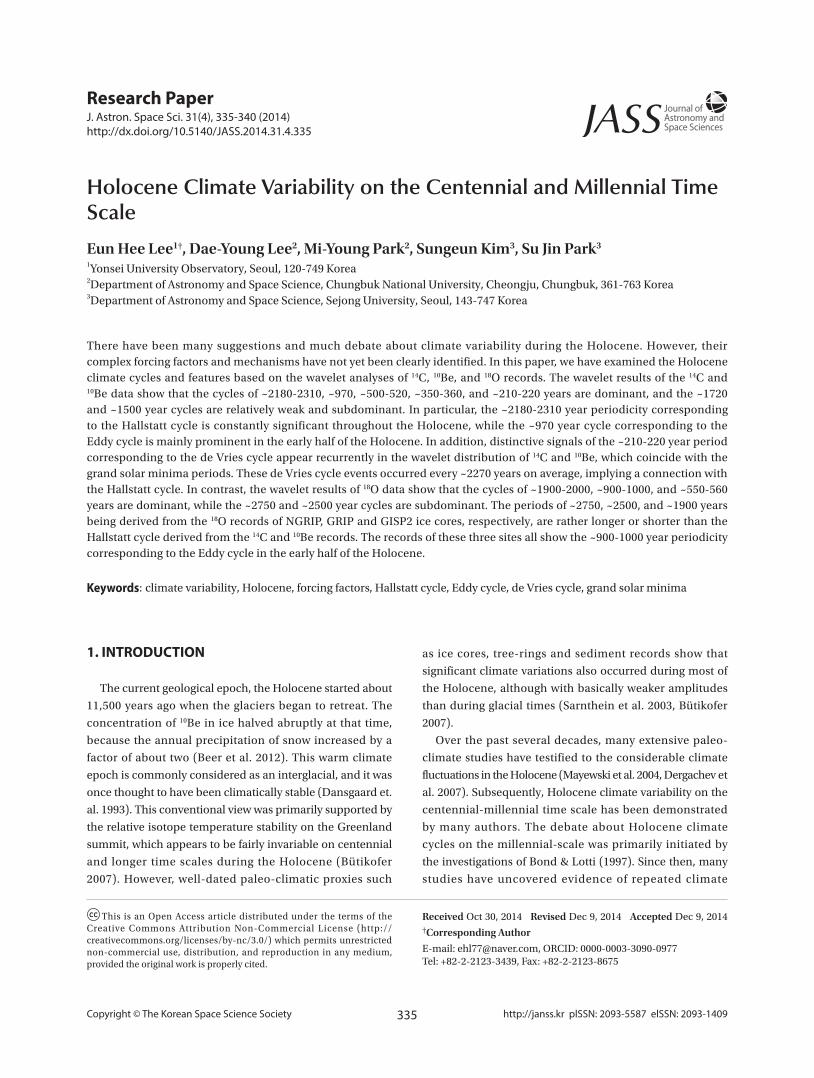
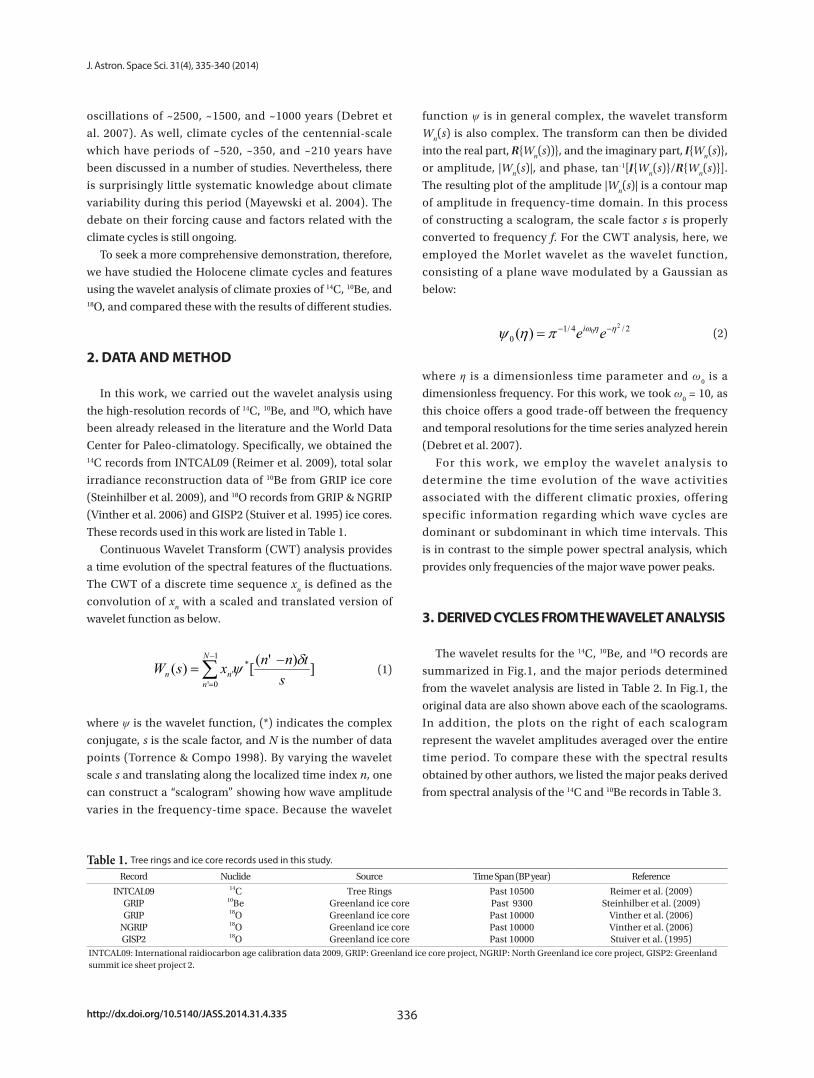
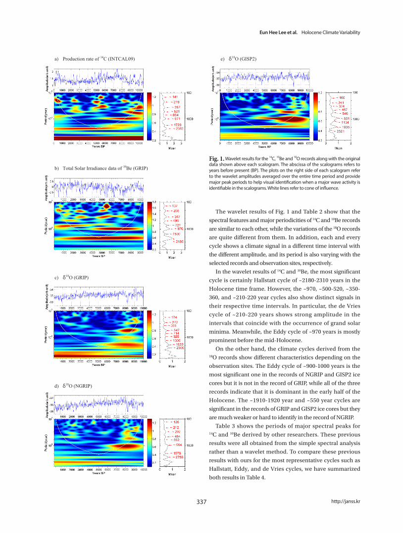
The wavelet results for the 14C, 10Be, and 18O records are

summarized in Fig.1, and the major periods determined

from the wavelet analysis are listed in Table 2. In Fig.1, the

original data are also shown above each of the scaolograms.

In addition, the plots on the right of each scalogram

represent the wavelet amplitudes averaged over the entire

time period. To compare these with the spectral results

obtained by other authors, we listed the major peaks derived

from spectral analysis of the 14C and 10Be records in Table 3.

Table 1. Tree rings and ice core records used in this study.

Record Nuclide Source Time Span (BP year) Reference

INTCAL09GRIPGRIP

NGRIPGISP2

14C10Be18O18O18O

Tree RingsGreenland ice coreGreenland ice coreGreenland ice coreGreenland ice core

Past 10500Past 9300Past 10000Past 10000Past 10000

Reimer et al. (2009)Steinhilber et al. (2009)

Vinther et al. (2006)Vinther et al. (2006)Stuiver et al. (1995)

INTCAL09: International raidiocarbon age calibration data 2009, GRIP: Greenland ice core project, NGRIP: North Greenland ice core project, GISP2: Greenland summit ice sheet project 2.

337 http://janss.kr

Eun Hee Lee et al. Holocene Climate Variability

The wavelet results of Fig. 1 and Table 2 show that the

spectral features and major periodicities of 14C and 10Be records

are similar to each other, while the variations of the 18O records

are quite different from them. In addition, each and every

cycle shows a climate signal in a different time interval with

the different amplitude, and its period is also varying with the

selected records and observation sites, respectively.

In the wavelet results of 14C and 10Be, the most significant

cycle is certainly Hallstatt cycle of ~2180-2310 years in the

Holocene time frame. However, the ~970, ~500-520, ~350-

360, and ~210-220 year cycles also show distinct signals in

their respective time intervals. In particular, the de Vries

cycle of ~210-220 years shows strong amplitude in the

intervals that coincide with the occurrence of grand solar

minima. Meanwhile, the Eddy cycle of ~970 years is mostly

prominent before the mid-Holocene.

On the other hand, the climate cycles derived from the 18O records show different characteristics depending on the

observation sites. The Eddy cycle of ~900-1000 years is the

most significant one in the records of NGRIP and GISP2 ice

cores but it is not in the record of GRIP, while all of the three

records indicate that it is dominant in the early half of the

Holocene. The ~1910-1920 year and ~550 year cycles are

significant in the records of GRIP and GISP2 ice cores but they

are much weaker or hard to identify in the record of NGRIP.

Table 3 shows the periods of major spectral peaks for 14C and 10Be derived by other researchers. These previous

results were all obtained from the simple spectral analysis

rather than a wavelet method. To compare these previous

results with ours for the most representative cycles such as

Hallstatt, Eddy, and de Vries cycles, we have summarized

both results in Table 4.

a) Production rate of 14C (INTCAL09)

b) Total Solar Irradiance data of 10Be (GRIP)

c) δ18O (GRIP)



c) δ18O (GRIP)



c) δ18O (GRIP)

d) δ18O (NGRIP)

e) δ18O (GISP2)

Fig. 1. Wavelet results for the 14C, 10Be and 18O records along with the original data shown above each scalogram. The abscissa of the scalograms refers to years before present (BP). The plots on the right side of each scalogram refer to the wavelet amplitudes averaged over the entire time period and provide major peak periods to help visual identification when a major wave activity is identifiable in the scalograms. White lines refer to cone of influence.

d) δ18O (NGRIP)

e) δ18O (GISP2)



Table 4 indicates that our wavelet results are overall

in good agreement with the previous spectral results for

each cycle. However, the period of each climate cycle is

variable in both analyses up to several percentages, in

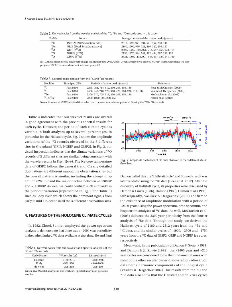
particular for the Hallstatt cycle. Fig. 2 shows the amplitude

variations of the 18O records observed in the 3 different

sites in Greenland (GRIP, NGRIP and GISP2). In Fig. 2, our

visual inspection indicates that the climate variations of 18O

records of 3 different sites are similar, being consistent with

the wavelet results in Figs. 1(c-e). The ice core temperature

data of GISP2 follows the general trend. Clearly detailed

fluctuations are different among the observation sites but

the overall pattern is similar, including the abrupt drop

around 8200 BP and the major decline between ~10000BP

and ~11000BP. As well, we could confirm such similarity in

the periodic variation (represented in Fig. 1 and Table 3)

such as Eddy cycle which shows the dominant signals from

early to mid-Holocene in all the 3 different observation sites.

4. FEATURES OF THE HOLOCENE CLIMATE CYCLES

In 1982, Chuck Sonnet employed the power spectrum

analysis to demonstrate that there was a ~2000 year periodicity

in the rather limited 14C data available at that time. He and Paul

Damon called this the “Hallstatt cycle” and Sonnet’s result was

later validated using the 10Be data (Beer et al. 2012). After the

discovery of Hallstatt cycle, its properties were discussed by

Damon & Linick (1986), Damon (1988), Damon et al. (1990).

Subsequently, Vasiliev & Dergachev (2002) confirmed

the existence of amplitude modulation with a period of

~2400 years using the power spectrum, time spectrum, and

bispectrum analyses of 14C data. As well, McCracken et al.

(2005) deduced the 2300 year periodicity from the Fourier

analysis of 10Be data. Through this study, we derived the

Hallstatt cycle of 2180 and 2312 years from the 10Be and 14C data, and the similar cycles of ~1900, ~2500 and ~2750

years from the 18O data of GISP2, GRIP and NGRIP ice cores,

respectively.

Meanwhile, in the publications of Damon & Sonett (1991)

and Damon & Jirikowie (1992), the ~2400 year and ~210

year cycles are considered to be the fundamental ones with

most of the other secular cycles discovered in radiocarbon

data being harmonic components of the longest cycle

(Vasiliev & Dergachev 2002). Our results from the 14C and 10Be data also show that the Hallstatt and de Vries cycles

Table 3. Spectral peaks derived from the 14C and 10Be records.

Nuclide Time Span (BP) Periods of major peaks (years) Reference14C14C10Be14C & 10Be

Past 9300Past 8000Past 9300Past 9400

2275, 984, 714, 512, 350, 208, 150, 1302400, 940, 710, 570, 500, 420, 360, 230, 210, 1902300, 970, 705, 515, 350, 208, 150, 1302200, 1000, 506, 208, 150

Beer & McCracken (2009)Vasiliev & Dergachev (2002)McCracken et al. (2005)Abreu et al. (2012)

Notes. Abreu et al. (2012) derived the cycles from the solar modulation potential Ф using the 14C & 10Be records.

Table 2. Derived cycles from the wavelet analysis of the 14C, 10Be and 18O records used in this paper.

Nuclide Source Average periods of the major peaks (years)14C

10Be18O18O18O

INTCAL09 (Production rate)GRIP (Total Solar Irradiance)GRIP (δ18O)NGRIP (δ18O)GISP2 (δ18O)

2312, 1720, 971, 694, 521, 357, 218, 1412180, 1500, 976, 721, 496, 347, 208, 1372500, 1920, 1300, 925, 714, 547, 355, 272, 1742756, 1976, 994, 741, 592, 464, 297, 212, 1262521, 1908, 1134, 901, 546, 467, 324, 241, 160

INTCAL09: International raidiocarbon age calibration data 2009, GRIP: Greenland ice core project, NGRIP: North Greenland ice core project, GISP2: Greenland summit ice sheet project 2.

Table 4. Derived cycles from the wavelet and spectral analyses of the 14C and 10Be records.

Cycle Name WA results (yr) SA results (yr)

HallstattEddy

de Vries

~2180-2312~971-976~208-218

~2200-2400~940-1000~208-210

Notes. WA: Wavelet analysis in this work, SA: Spectral analysis in previous studies

Fig. 2. Amplitude oscillations of 18O data observed in the 3 different sites in Greenland.

339 http://janss.kr

Eun Hee Lee et al. Holocene Climate Variability

are dominant during the Holocene, and the de Vries

cycle of ~210-220 years corresponds to the occurrence of

grand solar minima presented by Usoskin et al. (2007).

This feature was also indicated by Abreu et al. (2012) who

noticed that the amplitude of the ~210 year cycle is greatest

during the periods when grand solar minima are more

frequent. Related with this feature, there is an interesting

demonstration as follows: When the estimated solar

modulation function by Castagnoli & Lal (1980), ФCL80

is

filtered with a 1000-year running average, groups of deep

minima occur at 400 BP, 3100 BP, 5300 BP and 7300 BP.

Thus, these deep minima clusters occur with a periodicity

of (7300-400)/3 = 2300 years. That is, the ~2300 year

periodicity first detected by Sonnet was a consequence of

2300 year recurrence of clusters of grand minima (Beer et al.

2012). This is not precisely consistent with, but seems to be

overall in a qualitative agreement with our wavelet results

in Figs. 1a and 1b (i.e., ~ 500, ~2500, ~5300 and ~7300 BP).

In conclusion, therefore, we may infer that the Hallstatt and

de Vries cycles are in close relation with the appearance of

group of grand minima.

In addition, Eddy cycle also shows some difference

between wavelet and spectral analysis, and also among

the 14C, 10Be, and 18O records. Interestingly, however, all

the records of 14C, 10Be, and 18O reveal that Eddy cycle is

predominant during the early half of the Holocene.

5. SUMMARY AND DISCUSSION

In this paper, we focused on determining Holocene

climate cycles, especially on the centennial to millennial

time scales. Through our analyses, we confirmed most

major periodicities of centennial and millennial scales

which have been discussed in the previous studies. In

conclusion, this work reveals the following features:

1) The dominant cycles and features of 14C and 10Be data

show strong similarity and the same overall patterns

throughout the Holocene. But the climate variations

of 18O records show somewhat different characteristics

compared to 14C and 10Be.

2) The wavelet results of 14C and 10Be show that the most

conspicuous cycles are the ~2180-2310 and ~970 year

periodicities on the millennial scale, and the ~350-

360 and ~210-220 year cycles on the centennial scale.

In particular, the Hallstatt cycle of ~2180-2310 years

is significant throughout the Holocene, whereas the

Eddy cycle of ~970 years is conspicuous in the early

half of the Holocene

3) In contrast, 18O records show that the predominant

climate cycles are ~1900-2000 and ~900-1000 year

periodicities on the millennial scale, and the ~550-600

year cycle on the centennial scale. The period of ~1900,

~2500 and ~2750 years derived from the 18O records of

GISP2, GRIP and NGRIP ice cores, respectively, might

correspond to the Hallstatt cycles. The Eddy cycle

derived from the 3 different sites shows the period of

~900-1000 years in the early half of the Holocene

4) The de Vries cycle of ~210-220 years shows distinct

signals in the intervals centered on ~500, ~2500, ~5300

and ~7300 BP, being separated by ~ 2270 years on

average. Each of them coincides with the occurrence

of grand solar minima. Thus, it is likely that the

Hallstatt and de Vries cycles derived from the 14C and 10Be records are closely related with the appearance or

disappearance of grand solar minima, and also, there

is a link that implies a connection of the millennial

and centennial cycles between them. Therefore, it

seems that both of the Hallstatt and de Vries cycles are

directly connected with the solar activity.

5) On the other hand, abrupt event around 8200 BP

appeared in the 18O records, but did not show in the 14C and 10Be data. It is considered that it is probably not

related with solar forcing.

6) Lastly, this work indicates that the climate variations

such as the Hallstatt, Eddy, and de Vries cycles are

not only stationary oscillations, but also vary with

the proxy data, observational sites, and even analysis

methods to some extent.

ACKNOWLEDGEMENTS

This work was supported by the National Research

Foundation of Korea Grant funded by the Korean government

(NRF-2013-R1A1A3012194), and the work at Chungbuk

National University was supported by a NSL grant (NRF-2011-

0030742) from the National Research Foundation of Korea.

SJP of Sejong University was supported by Mid-career

Researcher Program through the National Research

Foundation of Korea (NRF) funded by the Ministry of

Education, Science, and Technology 2011-0028001.

REFERENCES

Abreu JA, Beer J, Ferriz-Mas A, McCracken KG, Steinhilber

F, Is there a planetary influence on solar activity?,

A&A 548, A88 (2012). http://dx.doi.org/10.1051/0004-

6361/201219997



Beer J, McCraken KG, Evidence for solar forcing: some

selected aspects. In Climate and Weather of the

Sun-Earth system (CAWSES), eds. Tsuda T, et al.

(TERRAPUB, Tokyo, 2009), 201-216.

Beer J, McCraken KG, von Steiger R, Cosmogenic Radionuclides

(Springer, London, 2012), 298-324. http://dx.doi.

org/10.1007/978-3-642-14651-0

Bond GC, Lotti R, Iceberg discharges into the North

Atlantic on millennial time scales during the last

glaciations, Science 267, 1005-1010 (1997). http://dx.doi.

org/10.1126/science.267.5200.1005

Bütikofer J, Millennial scale climate variability during

the last 6000 years - tracking down the Bond cycles,

Diploma thesis. University of Bern, 1-124 (2007).

Castagnoli G, Lal D, Solar modulation effects in terrestrial

production of carbon-14, Radiocarbon 22, 133-158

(1980).

Dansgaard W, Johnsen SJ, Clausen HB, Dahl J, Gundestrup

NS, et al., Evidence for General Instability of Past

Climate from a 250-kyr Ice-Core Record, Nature 364,

218-220 (1993). http://dx.doi.org/10.1038/364218a0

Damon PE, Production and decay radiocarbon and its

modulation by geomagnetic field-solar activity changes

with possible implications for global environment,

in Secular Solar and Geomagnetic Variations in the

Last 10000 years, eds. Stephenson FR, Wolfendale AW

(Kluwer, Dordrecht, 1988), 267-285.

Damon PE, Cheng S, Linick TW, Fine and hyperfine

structure in the spectrum of secular variations of

atmospheric 14C, Radiocarbon 31, 704-718 (1990).

Damon PE, Jirikowie JL, Radiocarbon evidence for low

frequency solar oscillation, in Rare Nuclear Processes,

ed. Povinec P, Proc. 14th Europhysics Conf. on Nuclear

Physics (Word Scientific Publishing Co, Singapore,

1992), 177-202.

Damon PE, Linick TW, Geomagnetic-heliomagnetic

modulation of atmospheric radiocarbon production,

Radiocarbon 28, 266-278 (1986).

Damon PE, Sonett CP, Solar and terrestrial components of

the atmospheric 14C variation spectrum, in The Sun in

time, eds. Sonett CP, Giampapa MS, and Mathews MS

(University of Arizona Press, Tucson, 1991), 360-388.

Debret M, Mout-Roumazeilles V, Grousset F, Desmet M,

Mcmanus JF, et al., The origin of the 1500-year climate

cycles in Holocene North-Atlantic records, Clim. Past 3,

569-575 (2007).

Dergachev VA, Raspopov OM, Damblon F, Jungner H,

Zaitseva GI, et al., Natural climate variability during the

Holocene, Radiocarbon 49, 837-854 (2007).

McCracken KG, Beer J, McDonald FB, The long-term

variability of the cosmogenic radiation intensity at

Earth as recorded by the cosmogenic nuclides, in The

solar system and beyond, ten years of ISSI, eds. Geiss J,

Hultqvist B (ESA Publication, the Netherlands, 2005),

83-98.

Mayewski PA, Rohling EE, Stager JC, Karlen W, Maasch

KA, et al., Holocene Climate Variability, Quaternary

Research 62, 243-255 (2004). http://dx.doi.org/10.1016/

j.yqres.2004.07.001

Reimer PJ, Baillie MGL, Bard E, Bayliss A, Beck JW, et al.,

IntCal09 and Marine09 radiocarbon age calibration

curves, 0-50 cal BP, Radiocarbon 51, 1111-1150 (2009).

Sarnthein M, Van Kreveld S, Erlenkeuser H, Grootes PM,

Kucera M, et al., Centennial-to-millennial-scale

periodicities of Holocene climate and sediment injections

off the western Barents shelf, 75 degrees N, Boreas 32, 447-

461 (2003). http://dx.doi.org/10.1111/j.1502-3885.2003.

tb01227.x

Steinhilber F, Beer J, Frohlich C, Total solar irradiance

during the Holocene, GRL 36, L19704 (2009). http://

dx.doi.org/10.1029/2009GL040142

Stuiver M, Pieter MG, Thomas FB, The GISP2 delta 18O

climate record of the past 16,500 years and the role of the

sun, ocean, and volcanoes, Quaternary Research 44, 341-

354 (1995). http://dx.doi.org/10.1006/qres.1995.1079

Torrence C, Compo GP, A practical guide to wavelet analysis,

Bull. Amer. Meteor. Soc. 79, 61-78 (1998). http://dx.doi.

org/10.1175/1520-0477(1998)079<0061:APGTWA>2.0.

CO;2

Usoskin IG, Solanki SK, Kovaltsov GA, Grand minima and

maxima of solar activity: new observational constraints,

A&A 471, 301-309 (2007). http://dx.doi.org/10.1051/0004-

6361:20077704

Vasiliev SS, Dergachev VA , The 2400-year cycle in

atmospheric radiocarbon concentration bispectrum

of 14C data over the last 8000 years, ANGEO 20, 115-120

(2002). http://dx.doi.org /10.5194/angeo-20-115-2002

Vinther BM, Clausen HB, Johnsen SJ, Rasmussen SO,

Andersen KK, et al., A synchronized dating of three

Greenland ice cores throughout the Holocene, JGR 111,

D13102 (2006). http://dx.doi.org/10.1029/2005JD006921

holocene climate variability on the centennial and

Documents