1

High-Fidelity Optimization of Flapping Airfoils for Maximum Propulsive Efficiency

Meilin Yu1 (�), Z. J. Wang2

The University of Kansas, Lawrence, KS 66045

and

Hui Hu3

Iowa State University, Ames, IA 50011

A high order spectral difference (SD) scheme based cost-effective multi-level optimization approach is proposed to optimize the kinematics of flapping airfoils and provide further insights into flapping motions with maximum propulsive efficiency. At the first stage, a gradient-based optimization algorithm is coupled with a second-order SD Navier-Stokes solver to search for the optimal kinematics of a certain airfoil undergoing a combined plunge and pitch motion. Then a high-order SD scheme is used to verify the optimization results and reveal the detailed vortex structures associated with the optimal kinematics of the flapping flight. Several NACA 4-digit airfoils are used in the optimization process. The maximum propulsive efficiency of oscillating NACA0006 and NACA0012 airfoils is more than 50% when the oscillating kinematics is optimized. The optimized propulsive efficiency of thin airfoils is larger than that of thick airfoils.

Nomenclature

� = pitching amplitude ��� = angle of attack � = speed of sound �� = specific heat at constant pressure ⟨����⟩ = time averaged power coefficient,

− � � ������������� + ����������� ��� !�"#$�

"# �0.5()*+ ��,

�� = thrust coefficient, -ℎ/01� �0.5()*2 ��⁄

⟨��⟩ = time averaged thrust coefficient, � � �����!�"#$�

"#

� = chord length 1Post-Doctoral Researcher, Department of Aerospace Engineering, AIAA Member, email: mlyu@ku.edu 2 Spahr Professor and Chair, Department of Aerospace Engineering, AIAA Associate Fellow, email: zjw@ku.edu 3 Associate Professor, Department of Aerospace Engineering, AIAA Associate Fellow, email: huhui@iastate.edu

51st AIAA Aerospace Sciences Meeting including the New Horizons Forum and Aerospace Exposition07 - 10 January 2013, Grapevine (Dallas/Ft. Worth Region), Texas

AIAA 2013-0085

Copyright © 2013 by Meilin Yu, Z. J. Wang, Hui Hu. Published by the American Institute of Aeronautics and Astronautics, Inc., with permission.

Dow

nloa

ded

by H

ui H

u on

Jan

uary

11,

201

3 | h

ttp://

arc.

aiaa

.org

| D

OI:

10.

2514

/6.2

013-

85

2

4 = total energy 5, 7 = vectors of fluxes in the physical domain 58, 78 = vectors of fluxes in the computational domain � = oscillation frequency 9 = inverse Hessian matrix ℎ = plunging amplitude �, : = index of coordinates in x, y direction ; = Jacobian matrix < = reduced frequency, 2>�� )*⁄ �� = Mach number ��* = Mach number of the free stream �� = mass flow rate �? , �@ = face normal components in A, � direction, respectively B/ = Prandtl number C = pressure C* = pressure of the free stream D,D8 = vectors of conservative variables in the physical and computational domains E� = Reynolds number based on the chord length, ()*� F⁄ G�/ = Strouhal number,2�ℎ )*⁄ �, I = time in the physical and computational domain 0, J = non-dimensional velocities in A, � direction JKL = grid velocity A, � = non-dimensional Cartesian coordinates in the physical domain AM , AN , AO, = metrics coefficients of the time-dependent coordinate transformation �M , �N , �O P = ratio of specific heats Q��� = propulsive efficiency, ⟨��⟩ ⟨�R��⟩⁄ � = pitching angle of the airfoil F = dynamic viscosity S, Q = Cartesian coordinates in the computational domain ( = density ITU = viscous stress tensors, �, : can be A or � ϕ = phase lag between pitching and plunging motions ω = angular frequency of oscillation, 2>�

1. Introduction Unsteady flapping-wing aerodynamics has attracted considerable research attention recently due to the increased interest in designing Micro Air Vehicles (MAVs) for a variety of missions, including reconnaissance and surveillance, targeting and sensing. Comprehensive reviews [1, 2, 3, 4, 5, 6, 7, 8] are available for the latest progress in this area, but there are still many missing pieces to the study of unsteady flapping flight. One of them is to find the flapping wing kinematics with the maximum efficiency and adequate aerodynamics performance.

Dow

nloa

ded

by H

ui H

u on

Jan

uary

11,

201

3 | h

ttp://

arc.

aiaa

.org

| D

OI:

10.

2514

/6.2

013-

85

3

Flapping motions can effectively generate thrust at low Reynolds and Mach numbers, and many research efforts have been devoted to shed light on the mechanism of efficient flapping flight. Jones and Platzer [9] argued that the combined plunge and pitch motion of flapping flight could adjust the effective angle of attack (AOA) of the airfoil, thus enhancing the thrust generation or power extraction performance. Anderson et al. [10] experimentally examined the propulsive performance of a NACA0012 airfoil with a combined plunge and pitch motion, and identified the parameters for an optimal thrust production. Isogai et al. [11] concluded from their results for a NACA0012 airfoil undergoing a combined plunge and pitch motion that a high propulsive efficiency can be obtained when the pitch leads plunge by 90 degrees and no apparent leading edge separation appeared. At the same time, Tuncer and Platzer [12] also found that high propulsive efficiency was achieved with an attached flow over the full period of the oscillation cycle for an NACA0012 airfoil. Note that in both cases the free stream Mach number was 0.3, which may be a bit large for the flapping wing simulations. Ramamurti and Sandberg [13] used a finite element incompressible flow solver to study an oscillating NACA0012 airfoil and investigated the effect of the phase difference between pitching and plunging motions on the thrust generation and propulsive efficiency. Kang et al. [14] used a Reynolds-Averaged Navier-Stokes (RANS) approach to study the flow over an oscillating SD7003 airfoil and examined the effects of turbulence models on the prediction of flow features. In addition, there has been a long-standing research interest in optimizing the kinematics of a flapping wing to achieve the optimal aerodynamic performance (in terms of lift, lift to drag ratio, thrust, propulsive efficiency, power consumption, etc.) in different scenarios. Jones [15] calculated the optimum load distribution along the wing for a given wing-root bending moment during the pure flapping motion, and found that the optimum loading was able to generate thrust more efficiently compared with an elliptic loading, which was suggested to be optimal for steady flight. Hall and Hall [16] computed the optimal circulation distribution along the span of flapping wings in fast forward flight using a 1D integral solution for small-amplitude motions and vortex-lattice techniques for large-amplitude motions. Ito [17] utilized vortex lattice method in conjunction with a hybrid optimization approach combining a genetic algorithm and sequential quadratic programming to optimize the flapping wing motion. A vortex lattice model was also adopted by other research groups [18, 19] as a suitable compromise between computational cost and accuracy, but it might fail to provide appropriate level of complexity of the motion when viscous effects became non-negligible [18]. In addition, Hamdaoui et al. [20] optimized the flapping kinematics for efficiency using a multi-objective evolutionary algorithm coupled with flapping flight physics models. The growing sophistication of computational hardware and simulation tools now allows for the direct coupling between optimization algorithms and high-fidelity Navier-Stokes solvers for the purpose of flapping motion optimization. Tuncer and Kaya [21] optimized the weighted sum consisting of thrust and propulsive efficiency of a flapping airfoil in combined plunging and pitching motion by coupling a gradient-based optimization method with a 2D Navier-Stokes solver supporting moving overset grids. Willis et al. [22] exploited a collection of computational tools with multiple fidelity levels in the design of effective flapping wing vehicles. In 2009, Pesavento and Wang [23] further confirmed that 2D flapping flight can be aerodynamically more efficient than the optimal steady motion.

Dow

nloa

ded

by H

ui H

u on

Jan

uary

11,

201

3 | h

ttp://

arc.

aiaa

.org

| D

OI:

10.

2514

/6.2

013-

85

4

Recently, Culbreth et al. [24] presented several optimization results for flapping airfoils and wings obtained from an optimization framework constructed by a gradient-based optimization algorithm and a low-dissipation kinetic energy preserving (KEP) finite volume Navier-Stokes solver. They found that the maximum propulsive efficiency appeared to occur right before the incipience of leading edge separation. In the present study, we propose to take a cost-effective multi-level optimization approach to provide further insights into flapping motions with maximum propulsive efficiency. At the first stage, a gradient-based optimization algorithm is coupled with a second-order spectral difference (SD) Navier-Stokes solver to search for the optimal kinematics of several NACA 4-digit airfoils undergoing a combined plunging and pitching motion. Since it is obvious that high-order methods are more accurate than low-order counterparts for simulations of vortex-dominated flows (e.g. bio-inspired flows) [25], at the final stage, a high-order Navier-Stokes solver is used to verify the optimization results and reveal the detailed vortex structures associated with the optimal kinematics of the flapping flight with high-fidelity to help better understand the physics. The remainder of this paper is organized as follows. In Section 2, the optimization framework including the numerical method is introduced. Numerical results are displayed and discussed in section 3. Section 4 briefly concludes the present work. 2. Optimization Framework 2.1 Governing Equations

Numerical simulations are performed with an unsteady compressible Navier-Stokes solver using dynamic unstructured grids based high-order spectral difference (SD) method developed in [26]. The 2D unsteady compressible Navier-Stokes equations in conservation form read,

0,Q F G

t x y

∂ ∂ ∂+ + =∂ ∂ ∂

(1)

where D = �(, (0, (J, 4�� are the conserved variables, and F, G are the total fluxes including both the inviscid and viscous flux vectors, i.e., F =5T − 5Yand G =7T − 7Y, which takes the following form

( )

2

,i

u

p uF

uv

u E p

ρρ

ρ

+ = +

( )2 ,i

v

uvG

p v

v E p

ρρ

ρ

= + +

0

xxv

yx

pxx yx x

F

Cu v T

Pr

ττ

µτ τ

= + +

,

0

xyv

yy

pxy yy y

G

Cu v T

Pr

ττ

µτ τ

= + +

.

(2)

In Eq. (2), (is the fluid density, 0and Jare the Cartesian velocity components, C is the pressure, and 4 is the total energy, F is dynamic viscosity, �� is the specific heat at constant

Dow

nloa

ded

by H

ui H

u on

Jan

uary

11,

201

3 | h

ttp://

arc.

aiaa

.org

| D

OI:

10.

2514

/6.2

013-

85

5

pressure, B/ is the Prandtl number, and - is the temperature. The stress tensors in Eq. (2) take the following form

( ) 2 , 2 ,3 3

x y x yxx x yy y xy yx x y

u v u vu v v uτ µ τ µ τ τ µ

+ + = − = − = = +

. (3)

On assuming that the perfect gas law is obeyed, the pressure is related to the total initial

energy byE = ^_` +

2 ρ�u2 + v2� with constant P, which closes the solution system.

To achieve an efficient implementation, a time-dependent coordinate transformation from the physical domain ��, A, �� to the computational domain�I, S, Q�, as shown in Fig. 1. (a), is applied to Eq. (1). And we obtain

0,Q F G

x yτ∂ ∂ ∂+ + =∂ ∂ ∂

ɶ ɶɶ

(4)

where

( )( )

x y

x y

Q J Q

F J Q F G

G J Q F G

τ

τ

ξ ξ ξ

η η η

= = + +

= + +

ɶ

ɶ

ɶ

. (5)

Herein, I = � and �S, Q� ∈ e−1,1g2, are the local coordinates in the computational domain. In the transformation shown above, the Jacobian matrix ; takes the following form

( )( )

, ,

, ,

0 0 1

x x xx y t

J y y yξ η τ

ξ η τξ η τ

∂ = = ∂

. (6)

Note that the grid velocity JKL = �A", �"� is related with �SM , QM� by

g

g

v

v

τ

τ

ξ ξη η

= − ∇

= − ∇ i

�i�

. (7)

2.2 Space Discretization

The SD method is used for the space discretization. In the SD method, two sets of points are given, namely the solution and flux points, as shown in Fig. 1. (b). Conservative variables are defined at the solution points (SPs), and then interpolated to flux points to calculate local fluxes. In the present study, the solution points are chosen as the Chebyshev-Gauss quadrature points and the flux points are selected to be the Legendre-Gauss points with end points as -1 and 1. Then using Lagrange polynomials, we reconstruct all the fluxes at the flux points. Note that this reconstruction is continuous within a standard element, but discontinuous on the cell interfaces. Therefore, for the inviscid flux, a Riemann solver is necessary to reconstruct a common flux on the interface. The reconstruction of the viscous flux is based on the average of the ‘left’ and ‘right’ fluxes. The detailed reconstruction procedures can be found in [26].

Dow

nloa

ded

by H

ui H

u on

Jan

uary

11,

201

3 | h

ttp://

arc.

aiaa

.org

| D

OI:

10.

2514

/6.2

013-

85

6

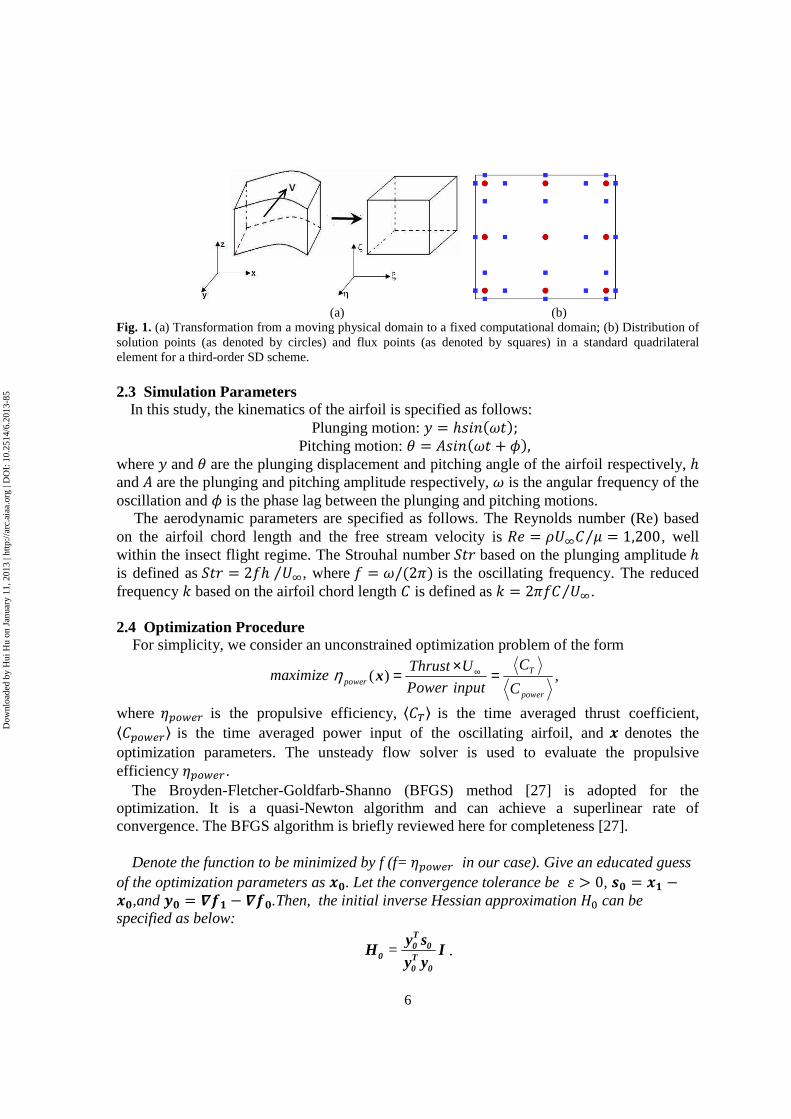
(a) (b) Fig. 1. (a) Transformation from a moving physical domain to a fixed computational domain; (b) Distribution of solution points (as denoted by circles) and flux points (as denoted by squares) in a standard quadrilateral element for a third-order SD scheme.

2.3 Simulation Parameters

In this study, the kinematics of the airfoil is specified as follows: Plunging motion: � = ℎ1���h��;

Pitching motion: � = �1���h� + j�, where � and � are the plunging displacement and pitching angle of the airfoil respectively, ℎ and � are the plunging and pitching amplitude respectively, h is the angular frequency of the oscillation and j is the phase lag between the plunging and pitching motions.

The aerodynamic parameters are specified as follows. The Reynolds number (Re) based on the airfoil chord length and the free stream velocity is E� = ()*� F⁄ = 1,200, well within the insect flight regime. The Strouhal number G�/ based on the plunging amplitude ℎ is defined as G�/ = 2�ℎ )*⁄ , where � = h/�2>� is the oscillating frequency. The reduced frequency < based on the airfoil chord length � is defined as < = 2>�� )*⁄ . 2.4 Optimization Procedure

For simplicity, we consider an unconstrained optimization problem of the form

maximize ( ) ,

power

Tpower

CThrust U

Powe Cr inputη ∞×= =x

where Q��� is the propulsive efficiency, ⟨��⟩ is the time averaged thrust coefficient, ⟨����⟩ is the time averaged power input of the oscillating airfoil, and l denotes the optimization parameters. The unsteady flow solver is used to evaluate the propulsive efficiency Q���.

The Broyden-Fletcher-Goldfarb-Shanno (BFGS) method [27] is adopted for the optimization. It is a quasi-Newton algorithm and can achieve a superlinear rate of convergence. The BFGS algorithm is briefly reviewed here for completeness [27].

Denote the function to be minimized by f (f=Q��� in our case). Give an educated guess of the optimization parameters as lm. Let the convergence tolerance be n > 0, pm = lq −lm,and rm = stq − stm.Then, the initial inverse Hessian approximation 9u can be specified as below:

=T0 0

0 T0 0

y sH I

y y.

Dow

nloa

ded

by H

ui H

u on

Jan

uary

11,

201

3 | h

ttp://

arc.

aiaa

.org

| D

OI:

10.

2514

/6.2

013-

85

7

Let < = 0, while ‖stw‖ > n, Compute line search direction

= −k k kp H f∇∇∇∇ .

Set lw$q = lw + xyzw, where xy is the line search step length, which satisfies the Wolfe condition,

1( ) ( )k kf f cα α+ ≤ + Tk k k k kx p x f p∇∇∇∇ ;

2( )Tk cα+ ≥ T

k k k k kf x p p f p∇ ∇∇ ∇∇ ∇∇ ∇ .

Update pw, rw, and {w$q using the following formulas: pw = lw$q − lw

rw = stw$q − stw

( ) ( )= - - +T T Tk+1 k k k k k k k k k kH I ρ s y H I ρ y s ρ s s ,

where (y = 1 |rw}pw~⁄ . < = < + 1 end (while)

Typical values for � and �2 in the Wolfe condition suggested in Ref. [27] are � = 10`� and �2 = 0.9. In the present optimization, a relatively large line search step length is used, namely xy = 1.0. If the Wolfe condition is not satisfied, then a contraction ratio 0.1 is multiplied to xy to limit the step size. 3. Optimization Results and Discussions

Since airfoils with different thickness may vary in aerodynamic performance [28], three NACA 4-digit airfoils, namely NACA0006, NACA0012 and NACA0030, in a combined plunge and pitch motion are used for the optimization. Optimization variables are taken to be the kinematics parameters, i.e. the phase shift between plunge and pitch motions j, the pitch and plunge amplitudes �, ℎ and the oscillation angular frequency h. The convergence criteria n for �Q����2is set as 10`�.

3.1 Optimization with one to three parameters

First of all, optimization with one to three parameters is carried out on the NACA0012 airfoil. Initial values of the optimization variables are chosen based on the previous study [29] for several NACA 4-digit airfoils in a combined plunge and pitch motion. 3.1.1 Optimization of j at G�/ = 0.3, < = 3.5 and � = 20�

The initial condition for this case is specified as j = 75�. The convergence histories of the �2 norm of ∇Q and j are shown in Fig. 2. The optimized phase lag j is 87.8� and the propulsive efficiency is 30.8%. From the convergence path, it is clear that the propulsive efficiency increases about 3% as j increases form 75� to 87.8� . Note that the optimal propulsive efficiency is achieved after only six optimization iterations.

Dow

nloa

ded

by H

ui H

u on

Jan

uary

11,

201

3 | h

ttp://

arc.

aiaa

.org

| D

OI:

10.

2514

/6.2

013-

85

8

(a) (b) Fig. 2. Convergences of (a) the �2 norm of ∇Q and (b) the phase lag j. 3.1.2 Optimization of �j, �� at G�/ = 0.3, < = 3.5

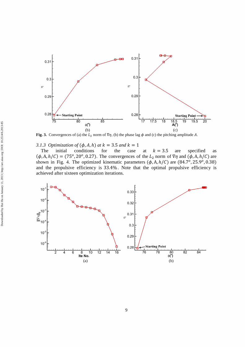
The initial conditions for this case are specified as �j, A� = �75� , 20�� . The convergences of the �2 norm of ∇Q and �j, A� are shown in Fig. 3. The optimized kinematic parameters �j, A� are �89.2� , 17.9�� and the propulsive efficiency is 31.2%. Note that the optimal propulsive efficiency is achieved after eight optimization iterations.

(a)

Dow

nloa

ded

by H

ui H

u on

Jan

uary

11,

201

3 | h

ttp://

arc.

aiaa

.org

| D

OI:

10.

2514

/6.2

013-

85

9

(b) (c) Fig. 3. Convergences of (a) the �2 norm of ∇Q, (b) the phase lag j and (c) the pitching amplitude �.

3.1.3 Optimization of �j, �, ℎ� at < = 3.5 and < = 1

The initial conditions for the case at < = 3.5 are specified as �j, A, ℎ/�� = �75� , 20� , 0.27�. The convergences of the �2 norm of ∇Q and �j, A, ℎ/�� are shown in Fig. 4. The optimized kinematic parameters �j, A, ℎ/�� are �84.7�, 25.9� , 0.38� and the propulsive efficiency is 33.4% . Note that the optimal propulsive efficiency is achieved after sixteen optimization iterations.

(a) (b)

Dow

nloa

ded

by H

ui H

u on

Jan

uary

11,

201

3 | h

ttp://

arc.

aiaa

.org

| D

OI:

10.

2514

/6.2

013-

85

10

(c) (d) Fig. 4. Convergences of (a) the �2 norm of ∇Q, (b) the phase lag j, (c) the pitching amplitude � and (d) the normalized plunging amplitude ℎ/� at < = 3.5.

The initial conditions for the case at < = 1 are specified as �j, A, ℎ/�� = �85�, 46�, 1.5�. The convergences of the �2 norm of ∇Q and �j, A, ℎ/�� are shown in Fig. 5. The optimized kinematic parameters �j, A, ℎ/�� are �86.4� , 49.0� , 1.66� and the propulsive efficiency is 53.3%. In this case, the gradient of the propulsive efficiency ∇Q does not converge to the desired error level but the values of j, A, ℎ/� converge almost surely towards the local minima. Therefore, the optimization results are reasonable.

(a) (b)

Dow

nloa

ded

by H

ui H

u on

Jan

uary

11,

201

3 | h

ttp://

arc.

aiaa

.org

| D

OI:

10.

2514

/6.2

013-

85

11

(c) (d) Fig. 5. Convergences of (a) the �2 norm of ∇Q, (b) the phase lag j, (c) the pitching amplitude � and (d) the normalized plunging amplitude ℎ/� at < = 1. 3.2 Optimization with four parameters

In this section, optimization with four parameters is carried out on NACA0006, NACA0012 and NACA0030 airfoils. The flow fields with the optimized kinematics parameters are then simulated using a 3rd order SD scheme. The corresponding aerodynamic force histories are then analyzed to elucidate various performances of different airfoils.

3.2.1 Optimization of �j, �, ℎ, h�

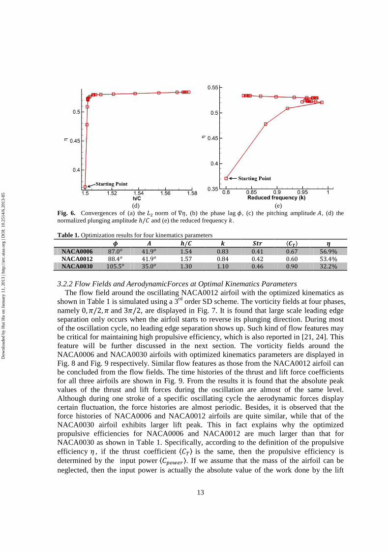
The initial conditions for the case are specified as �j, A, ℎ �⁄ , <� = �85� , 46� , 1.5, 0.8�. The convergences of the �2 norm of ∇Q and �j, A, ℎ/�� for NACA0012 are shown in Fig. 6. The optimized kinematic parameters �j, A, ℎ �⁄ , <� are �88.4�, 41.9� , 1.57,0.84� and the propulsive efficiency is 53.4%. As the optimization at < = 1 in Section 3.1.3, the gradient of the propulsive efficiency ∇Q does not converge to the desired error level but the values of j, A, ℎ/� and < converge almost surely towards the local minima. Note that the optimized propulsive efficiency in this case is quite similar to the case at < = 1 in Section 3.1.3. However, the optimized kinematic parameters in this case are not very close to those in Section 3.1.3. This might indicate that there exists a parametric region in which all the propulsive efficiencies are quite similar to the optimal one. Besides, by comparing all the optimization cases for NACA0012, it is found that when the reduced frequency decreases to about 1, the propulsive efficiency achieves a large value and the optimization problem then becomes ‘stiff’.

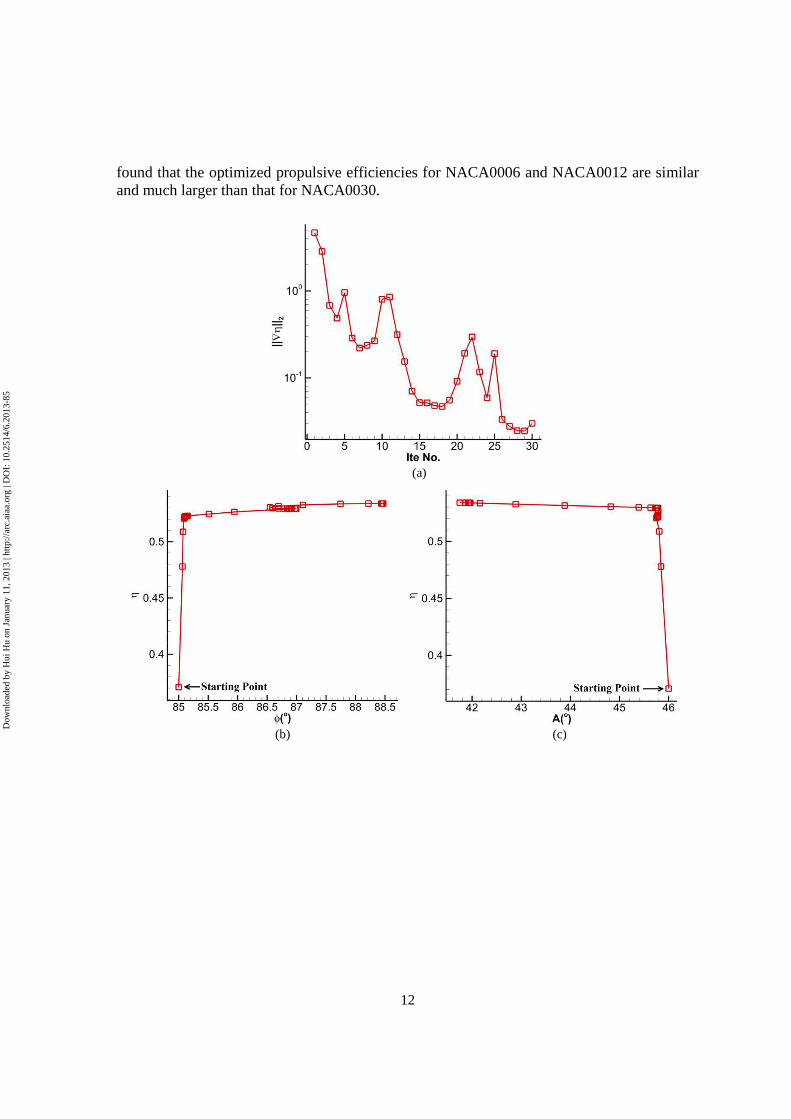
On using the same initial conditions of �j, A, ℎ �⁄ , <� as shown above, the optimized kinematics parameters for the oscillating NACA0006 and NACA0030 airfoil is obtained as �j, A, ℎ �⁄ , <� = �87.0� , 41.9� , 1.54, 0.83� and �105.5�, 35.0� , 1.30, 1.10�. The maximized propulsion efficiencies are 56.9% and 32.2% repectively. Similarly to the optimization process of the NACA0012 airfoil, the gradient of the propulsive efficiencies ∇Q for both NACA0006 and NACA0030 airfoils do not converge to the desired error level but the values of j, A, ℎ/� and < converge almost surely towards the local minima. All the results for the optimization with four parameters are summarized in Table 1. From this table, it is also

Dow

nloa

ded

by H

ui H

u on

Jan

uary

11,

201

3 | h

ttp://

arc.

aiaa

.org

| D

OI:

10.

2514

/6.2

013-

85

12

found that the optimized propulsive efficiencies for NACA0006 and NACA0012 are similar and much larger than that for NACA0030.

(a)

(b) (c)

Dow

nloa

ded

by H

ui H

u on

Jan

uary

11,

201

3 | h

ttp://

arc.

aiaa

.org

| D

OI:

10.

2514

/6.2

013-

85

13

(d) (e) Fig. 6. Convergences of (a) the �2 norm of ∇Q, (b) the phase lag j, (c) the pitching amplitude �, (d) the normalized plunging amplitude ℎ/� and (e) the reduced frequency <. Table 1. Optimization results for four kinematics parameters

� � �/� w ��� ⟨�}⟩ � NACA0006 87.0� 41.9� 1.54 0.83 0.41 0.67 56.9% NACA0012 88.4� 41.9� 1.57 0.84 0.42 0.60 53.4% NACA0030 105.5� 35.0� 1.30 1.10 0.46 0.90 32.2%

3.2.2 Flow Fields and AerodynamicForces at Optimal Kinematics Parameters

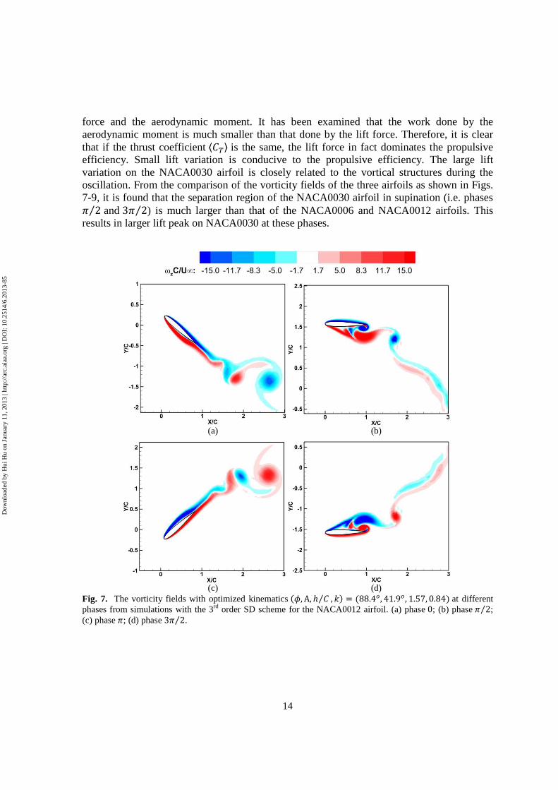
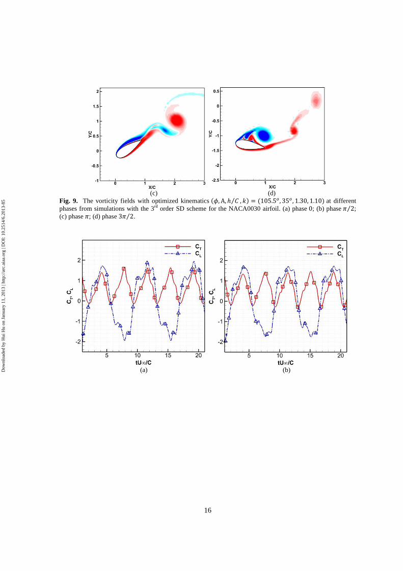
The flow field around the oscillating NACA0012 airfoil with the optimized kinematics as shown in Table 1 is simulated using a 3rd order SD scheme. The vorticity fields at four phases, namely 0, >/2, > and 3>/2, are displayed in Fig. 7. It is found that large scale leading edge separation only occurs when the airfoil starts to reverse its plunging direction. During most of the oscillation cycle, no leading edge separation shows up. Such kind of flow features may be critical for maintaining high propulsive efficiency, which is also reported in [21, 24]. This feature will be further discussed in the next section. The vorticity fields around the NACA0006 and NACA0030 airfoils with optimized kinematics parameters are displayed in Fig. 8 and Fig. 9 respectively. Similar flow features as those from the NACA0012 airfoil can be concluded from the flow fields. The time histories of the thrust and lift force coefficients for all three airfoils are shown in Fig. 9. From the results it is found that the absolute peak values of the thrust and lift forces during the oscillation are almost of the same level. Although during one stroke of a specific oscillating cycle the aerodynamic forces display certain fluctuation, the force histories are almost periodic. Besides, it is observed that the force histories of NACA0006 and NACA0012 airfoils are quite similar, while that of the NACA0030 airfoil exhibits larger lift peak. This in fact explains why the optimized propulsive efficiencies for NACA0006 and NACA0012 are much larger than that for NACA0030 as shown in Table 1. Specifically, according to the definition of the propulsive efficiency Q , if the thrust coefficient ⟨��⟩ is the same, then the propulsive efficiency is determined by the input power ⟨����⟩. If we assume that the mass of the airfoil can be neglected, then the input power is actually the absolute value of the work done by the lift

Dow

nloa

ded

by H

ui H

u on

Jan

uary

11,

201

3 | h

ttp://

arc.

aiaa

.org

| D

OI:

10.

2514

/6.2

013-

85

14

force and the aerodynamic moment. It has been examined that the work done by the aerodynamic moment is much smaller than that done by the lift force. Therefore, it is clear that if the thrust coefficient ⟨��⟩ is the same, the lift force in fact dominates the propulsive efficiency. Small lift variation is conducive to the propulsive efficiency. The large lift variation on the NACA0030 airfoil is closely related to the vortical structures during the oscillation. From the comparison of the vorticity fields of the three airfoils as shown in Figs. 7-9, it is found that the separation region of the NACA0030 airfoil in supination (i.e. phases > 2⁄ and 3> 2⁄ ) is much larger than that of the NACA0006 and NACA0012 airfoils. This results in larger lift peak on NACA0030 at these phases.

(a) (b)

(c) (d) Fig. 7. The vorticity fields with optimized kinematics �j, A, ℎ �⁄ , <� = �88.4�, 41.9�, 1.57, 0.84� at different phases from simulations with the 3rd order SD scheme for the NACA0012 airfoil. (a) phase 0; (b) phase > 2⁄ ; (c) phase >; (d) phase 3> 2⁄ .

Dow

nloa

ded

by H

ui H

u on

Jan

uary

11,

201

3 | h

ttp://

arc.

aiaa

.org

| D

OI:

10.

2514

/6.2

013-

85

15

(a) (b)

(c) (d) Fig. 8. The vorticity fields with optimized kinematics �j, A, ℎ �⁄ , <� = �87.0�, 41.9�, 1.54, 0.83� at different phases from simulations with the 3rd order SD scheme for the NACA0006 airfoil. (a) phase 0; (b) phase > 2⁄ ; (c) phase >; (d) phase 3> 2⁄ .

(a) (b)

Dow

nloa

ded

by H

ui H

u on

Jan

uary

11,

201

3 | h

ttp://

arc.

aiaa

.org

| D

OI:

10.

2514

/6.2

013-

85

16

(c) (d) Fig. 9. The vorticity fields with optimized kinematics �j, A, ℎ �⁄ , <� = �105.5�, 35�, 1.30, 1.10� at different phases from simulations with the 3rd order SD scheme for the NACA0030 airfoil. (a) phase 0; (b) phase > 2⁄ ; (c) phase >; (d) phase 3> 2⁄ .

(a) (b) D

ownl

oade

d by

Hui

Hu

on J

anua

ry 1

1, 2

013

| http

://ar

c.ai

aa.o

rg |

DO

I: 1

0.25

14/6

.201

3-85

17

(c)

Fig. 10. Time histories of the thrust and lift force coefficients with optimized kinematics for the (a) NACA0006, (b) NACA0012 and (c) NACA0030 airfoils. 3.3 Discussion of the optimized kinematics

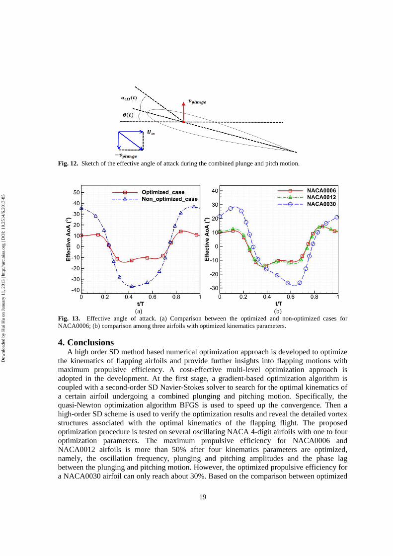
In this section, aerodynamic performance and the corresponding flow fields from the optimized and non-optimized cases around an oscillating NACA0006 airfoil are compared. From Table 2, it is clear that although the time averaged thrust coefficient is almost the same for these two cases, the propulsive efficiency for the optimized case is about 2.5 times of that for the non-optimized case. The vorticity fields with the non-optimized kinematics parameters at four phases are displayed in Fig. 11. It is obvious that large leading edge separation appears during the entire oscillation cycle. Also observed from Table 2, there exists apparent difference on the pitching amplitude between the optimized and non-optimized cases. This infers that the large leading edge separation form the non-optimized case could be connected with the variation of the effective AOA.

The definition of the effective AOA for the combined plunge and pitch motion is given as

x�� = �/���� � ��)*

� − �,

assuming that the pitch speed is negligible. Sketch of the effective AOA during the oscillation is shown in Fig. 12. The variation of the effective AOA for both optimized and non-optimized cases of NACA0006 is displayed in Fig. 13(a). It is obvious that for the optimized case, the peak absolute value of effective AOA is well controlled below 15�. This feature can help prevent the appearance of large leading edge separation. However for the non-optimized case, the peak absolute value of effective AOA can reach about 40� and during the entire oscillation cycle, the effective AOA remains at large value. Then a large leading edge separation appears during the entire oscillation cycle for the non-optimized case. The variation of the effective AOA for NACA0006, NACA0012 and NACA0030 airfoils with optimized kinematics parameters is shown in Fig. 13(b). It is clear that the variation trace for both NACA0006 and NACA0012 is quite similar, but different with that for NACA0030. It is also found that the peak absolute value of effective AOA of NACA0030 is

Dow

nloa

ded

by H

ui H

u on

Jan

uary

11,

201

3 | h

ttp://

arc.

aiaa

.org

| D

OI:

10.

2514

/6.2

013-

85

18

about 30� , which is twice that of the other two airfoils. Thus the lift generation on NACA0030 can be much larger than that on NACA0006 and NACA0012. Based on the analyses in Section 3.2.2, the lower optimized propulsive efficiency of NACA0030 can be attributed to the large variation of the effective AOA. Table 2. Comparison of kinematics parameters and aerodynamic performance of a NACA0006 airfoil with optimized and non-optimized kinematics parameters.

� � �/� w ��� ⟨�}⟩ � Non-optimized 75� 20� 1.41 1.0 0.45 0.70 20.8%

Optimized 87� 41.9� 1.54 0.83 0.41 0.67 56.9%

(a) (b)

(c) (d) Fig. 11. The vorticity fields with non-optimized kinematics at different phases from simulations with the 3rd SD scheme for the NACA0006 airfoil. (a) phase 0; (b) phase > 2⁄ ; (c) phase >; (d) phase 3> 2⁄ .

Dow

nloa

ded

by H

ui H

u on

Jan

uary

11,

201

3 | h

ttp://

arc.

aiaa

.org

| D

OI:

10.

2514

/6.2

013-

85

19

Fig. 12. Sketch of the effective angle of attack during the combined plunge and pitch motion.

(a) (b) Fig. 13. Effective angle of attack. (a) Comparison between the optimized and non-optimized cases for NACA0006; (b) comparison among three airfoils with optimized kinematics parameters.

4. Conclusions A high order SD method based numerical optimization approach is developed to optimize

the kinematics of flapping airfoils and provide further insights into flapping motions with maximum propulsive efficiency. A cost-effective multi-level optimization approach is adopted in the development. At the first stage, a gradient-based optimization algorithm is coupled with a second-order SD Navier-Stokes solver to search for the optimal kinematics of a certain airfoil undergoing a combined plunging and pitching motion. Specifically, the quasi-Newton optimization algorithm BFGS is used to speed up the convergence. Then a high-order SD scheme is used to verify the optimization results and reveal the detailed vortex structures associated with the optimal kinematics of the flapping flight. The proposed optimization procedure is tested on several oscillating NACA 4-digit airfoils with one to four optimization parameters. The maximum propulsive efficiency for NACA0006 and NACA0012 airfoils is more than 50% after four kinematics parameters are optimized, namely, the oscillation frequency, plunging and pitching amplitudes and the phase lag between the plunging and pitching motion. However, the optimized propulsive efficiency for a NACA0030 airfoil can only reach about 30%. Based on the comparison between optimized

Dow

nloa

ded

by H

ui H

u on

Jan

uary

11,

201

3 | h

ttp://

arc.

aiaa

.org

| D

OI:

10.

2514

/6.2

013-

85

20

and non-optimized cases for the NACA0006 airfoil, the variation of effective AOA plays a key role in achieving high propulsive efficiency. It is found that under optimized conditions, the variation of effective AOA is well controlled to avoid the occurrence of large leading edge separation during most of the oscillation cycle.

References

[1] S. Ho, H. Nassef, N. Pornsinsirirak, Y. C. Tai and C. M. Ho, "Unsteady aerodynamics and flow control for flapping wing flyers," Progress in Aerospace Sciences, vol. 39, no. 8, p. 635–681, 2003.

[2] M. F. Platzer, K. D. Jones, J. Young and J. C. S. Lai, "Flapping-wing aerodynamics: progress and challenges," AIAA J., vol. 46, no. 9, pp. 2136-2149, 2008.

[3] K. V. Rozhdestvensky and V. A. Ryzhov, "Aerohydrodynamics of flapping-wing propulsors," Progress in Aerospace Sciences, vol. 39, no. 8, pp. 585-633, 2003.

[4] W. Shyy, H. Aono, S. Chimakurthi, P. Trizila, C. Kang, C. Cesnik and H. Liu, "Recent progress in flapping wing aerodynamics and aeroelasticity," Progress in Aerospace Sciences, vol. 48, no. 7, pp. 284-327, 2010.

[5] W. Shyy, M. Berg and D. Ljungqvist, "Flapping and flexible wings for biological and micro air vehicles," Progress in Aerospace Sciences, vol. 35, no. 5, pp. 455-505, 1999.

[6] W. Shyy, Y. Lian, J. Tang, D. Viieru and H. Liu, Aerodynamics of low Reynolds number flyers, New York: Cambridge Univ. Press, 2008.

[7] M. S. Triantaflyllou, A. H. Techet and F. S. Hover, "Review of experimental work in biomimetic foils," IEEE Journal of Oceanic Engineering, vol. 29, no. 3, pp. 585-594, 2004.

[8] Z. J. Wang, "Dissecting insect flight," Annu. Rev. Fluid Mech., vol. 37, no. 1, pp. 183-210, 2005.

[9] K. D. Jones and M. F. Platzer, "Numerical computation of flapping-wing propulsion and power extraction," in AIAA Paper No. 97-0826, 1997.

[10] J. M. Anderson, K. Streitlien, D. S. Barrett and M. S. Triantafyllou, "Oscillating foils of high propulsive efficiency," J. Fluid Mech., vol. 360, pp. 41-72, 1998.

[11] K. Isogai, Y. Shinmoto and Y. Watanabe, "Effects of Dynamic Stall on Propulsive Efficiency and Thrust of Flapping Airfoil," AIAA J., vol. 37, no. 10, pp. 1145-1151, 1999.

[12] I. H. Tuncer and M. F. Platzer, "Computational study of flapping airfoil aerodynamics," Journal of Aircraft, vol. 37, no. 3, pp. 514-520, 2000.

[13] R. Ramamurti and W. Sandberg, "Simulation of flow about flapping airfoils using finite element incompressible flow solver," AIAA J., vol. 39, no. 2, pp. 253-260, 2001.

[14] C. K. Kang, H. Aono, P. Trizila, Y. Baik, J. M. Rausch, L. Bernal, M. V. Ol and W. Shyy, "Modeling of pitching and plunging airfoils at Reynolds number between 1×10^4 and 6×10^4," in AIAA Paper 2009-4100, 2009.

[15] R. T. Jones, "Wing Flapping with Minimum Energy," NASA Technical Memorandum 81174 , 1980.

[16] K. C. Hall and S. R. Hall, "Minimum induced power requirements for flapping flight," Journal of Fluid Mechanics, vol. 323, pp. 285-315, 1996.

[17] K. Ito, "Optimization of Flapping Wing Motion," in ICAS 2002 CONGRESS, 2002.

[18] B. K. Stanford and P. S. Beran, "Analytical Sensitivity Analysis of an Unsteady Vortex-Lattice Method for Flapping-Wing Optimization," Journal of Aircraft, vol. 47, no. 2, pp. 647-662, 2010.

Dow

nloa

ded

by H

ui H

u on

Jan

uary

11,

201

3 | h

ttp://

arc.

aiaa

.org

| D

OI:

10.

2514

/6.2

013-

85

21

[19] M. Ghommem, M. R. Hajj, L. T. Watson, D. T. Mook, R. D. Snyder and P. S. Beran, "Deterministic Global Optimization of Flapping Wing Motion for Micro Air Vehicles," in 2010 AIAA ATIO/ISSMO Conference, 2010.

[20] M. Hamdaoui, J.-B. Mouret, S. Doncieux and P. Sagaut, "Optimization of Kinematics for Birds and UAVs using Evolutionary Algorithms," World Academy of Science, Engineering and Technology, vol. 47, pp. 181-192, 2008.

[21] I. H. Tuncer and M. Kaya, "Optimization of Flapping Airfoils for Maximum Thrust and Propulsive Efficiency," AIAA Journal, vol. 43, no. 11, pp. 2329-2336, 2005.

[22] D. J. Willis, P.-O. Persson, E. R. Israeli, J. Peraire, S. M. Swartz and K. S. Breuer, "Multifidelity Approaches for the Computational Analysis and Design of Effective Flapping Wing Vehicles," in AIAA 2008-518, Reno, Nevada, 2008.

[23] U. Pesavento and Z. J. Wang, "FlappingWing Flight Can Save Aerodynamic Power Compared to Steady Flight," Physical Review Letters, vol. 103, pp. 118102-4, 2009.

[24] M. Culbreth, Y. Allaneau and A. Jameson, "High-Fidelity Optimization of Flapping Airfoils and Wings," in AIAA 2011-3521, Honolulu, Hawaii, 2011.

[25] Z. J. Wang, "High-order methods for the Euler and Navier Stokes equations on unstructured grids," Progress in Aerospace Science, vol. 43, pp. 1-41, 2007.

[26] M. L. Yu, Z. J. Wang and H. Hu, "A high-order spectral difference method for unstructured dynamic grids," Computer & Fluids, vol. 48, no. 1, pp. 84-97, 2011.

[27] J. Nocedal and S. Wright, Numerical optimization, Springer, 2000.

[28] M. L. Yu, Z. J. Wang and H. Hu, "Airfoil thickness effects on the thrust generation of plunging airfoils," Journal of Aircraft, vol. 49, no. 5, pp. 1434-1439, 2012.

[29] M. L. Yu, Z. J. Wang and H. Hu, "A high-fidelity numerical study of kinematics and airfoil thickness effects on the thrust generation of oscillating airfoils," in AIAA 2012-2966, New Orleans, Louisiana, 2012.

Dow

nloa

ded

by H

ui H

u on

Jan

uary

11,

201

3 | h

ttp://

arc.

aiaa

.org

| D

OI:

10.

2514

/6.2

013-

85