Hidden Markov Models

A Summary for

“A tutorial on Hidden Markov Models and Selected Applications in Speech Recognition,

by Lawrence R. Rabiner”

By Seçil Öztürk

Outline

●Signal Models●Markov Chains●Hidden Markov Models●Fundamentals for HMM Design●Types of HMMs

Signal Models...

●Are used to characterize real world signals.

●Provide a basis for a theoretical description of a signal processing system.

●Tell about the signal source without having the source available.

●Are used to realize practical systems efficiently.

2 Types of Signal Models:

●Deterministic Models:- Specific properties of the signal are known.

eg. The signal is a sine wave- Determining values for parameters of the signal, such as

frequency, amplitude, etc is required.

●Statistical Models:- eg. Gaussian processes, Markov processes, Hidden Markov

processes- Characterizing the statistical properties of the signal is

required. - Assumption:

* Signal can be characterized as a parametric random process.* Parameters of the random process can be determined in a

precise and well defined manner.

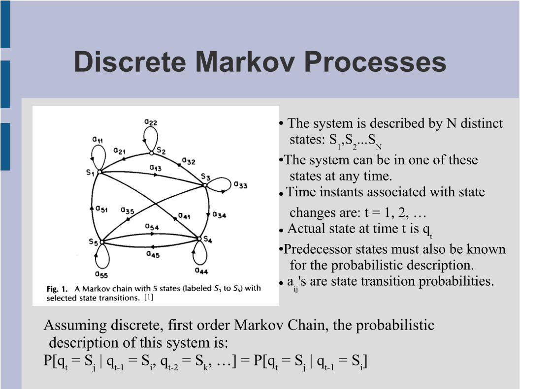
Discrete Markov Processes

[1]

● The system is described by N distinct states: S

1,S

2...S

N

●The system can be in one of these states at any time.

●

Time instants associated with state

changes are: t = 1, 2, …● Actual state at time t is q

t

●Predecessor states must also be known for the probabilistic description.

● aij's are state transition probabilities.

Assuming discrete, first order Markov Chain, the probabilistic description of this system is:

P[qt = S

j | q

t-1 = S

i, q

t-2 = S

k, …] = P[q

t = S

j | q

t-1 = S

i]

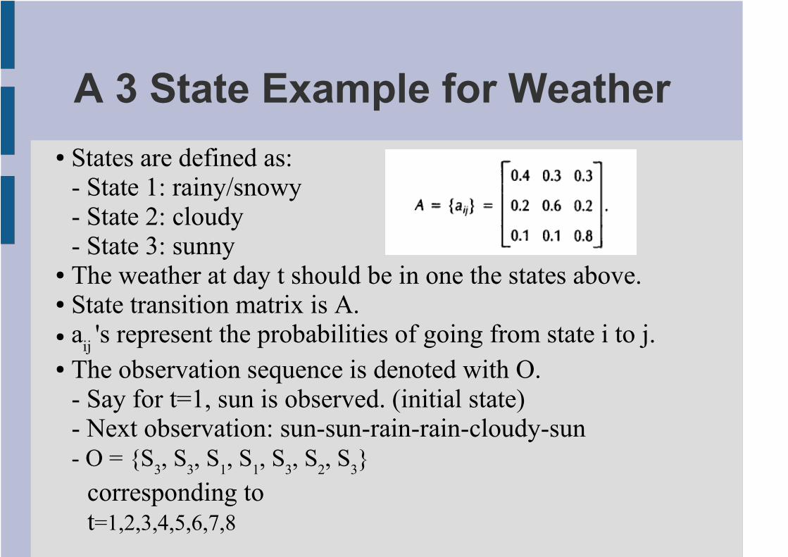
A 3 State Example for Weather

● States are defined as:- State 1: rainy/snowy- State 2: cloudy- State 3: sunny

● The weather at day t should be in one the states above.● State transition matrix is A.● a

ij 's represent the probabilities of going from state i to j.

● The observation sequence is denoted with O.- Say for t=1, sun is observed. (initial state)- Next observation: sun-sun-rain-rain-cloudy-sun- O = {S

3, S

3, S

1, S

1, S

3, S

2, S

3}

corresponding tot=1,2,3,4,5,6,7,8

A 3 State Example for Weather

● The probability of the observation sequence given the model is as follows:

here, πi's are the initial state probabilities.

Hidden Markov Models

* In Markov Models, states corresponded to observable/pyhsical events.

* In Hidden Markov Models,observations are probabilistic functions of the state.

- So, HMMs are doubly embedded stochastic processes.

- The underlying stochastic process is not observable/hidden. It can be observed through another set of stochastic processes producing the observation sequences.

(ie., in Markov Models, the problem is finding the probability of the observation to be in a certain state, in HMMs, the problem is still finding the probability of the observation to be in a certain state, but observation is also a probabilistic function of the state. )

eg. Hidden Coin Tossing Experiment, Urn and Ball Model

Elements of an HMM

● N: # of statesIndividual states: S = {S

1, … , S

N} State at time t: q

t

● M: (# of distinct observation symbols)/stateie. discrete alphabet size in speech processingeg. heads & tails in coins experimentindividual symbols: V = {v

1,v

2, ... , v

M}

● A: State transition prob. distributionaij = P[q

t+1= S

j | q

t=S

i] where 1 <= i, j <= N

● B: the observation symbol probability distribution in state jB = b

j(k) where b

j(k) = P[v

k at t|q

t=S

j] where

eg. The probability of heads of a certain coin at time t.● π = { π

i } is are the initial state distribution.

● πi =P[q

1 = S

i] where

*** Given N, M, A, B, π, HMM can be generated for O.● O : Observation sequence O = O

1,O

2, … , O

T. O

T''s are one of v

i's. T is #

of total observations.

Complete specification of an HMM requires:

* A,B,π: probability measures* N and M: model parameters* O: observation symbols

HMM notation: λ (A,B,π)

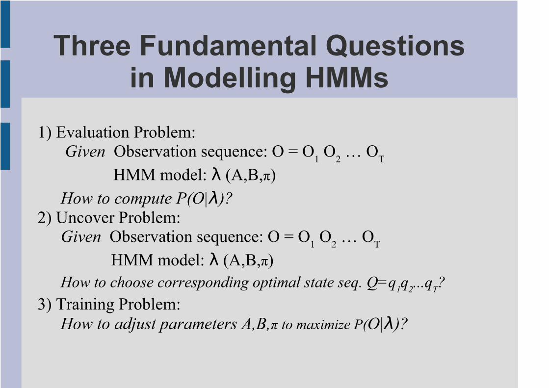
Three Fundamental Questions in Modelling HMMs

1) Evaluation Problem: Given Observation sequence: O = O

1 O

2 … O

T

HMM model: λ (A,B,π)

How to compute P(O|λ)?

2) Uncover Problem:Given Observation sequence: O = O

1 O

2 … O

T

HMM model: λ (A,B,π)How to choose corresponding optimal state seq. Q=q

1q

2...q

T?

3) Training Problem:How to adjust parameters A,B,π to maximize P(O|λ)?

Solution for Problem 1

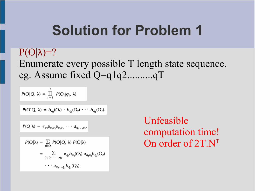
P(O|λ)=?Enumerate every possible T length state sequence.eg. Assume fixed Q=q1q2..........qT

Unfeasible computation time!On order of 2T.NT

Solution for Problem 1

Forward-Backward procedureForward variable: α

t(i)=P(O

1O

2....O

t,q

t=S

i|λ)

(prob. for partial observation sequence O1...O

t ending at state S

i at time t, λ)

Inductive Solution!

Computation time:On order of N2T

Trellis

α1(N)

α1(4)

α1(3)

α1(2)

α1(N)

α1(1) α

2(1)

α2(2)

α2(3)

α2(4)α

1(4)

α2(N) α

3(N)α

2(N) α

4(N) α

5(N) α

T(N)

αT(4)

αT(3)

αT(2)

αT(1)

α5(4)

α5(3)

α5(2)

α5(1)α

4(1)

α4(2)

α4(3)

α4(4)α

3(4)

α3(3)

α3(2)

α3(1)

Backward Variable:β

t(i)=P(O

t+1O

t+2...O

T|q

T=S

i,λ)

(probability of the partial observation sequence from t+1 to end, given state Si at time t, λ)

Inductive Solution!Computation time:On order of N2T

Solution for Problem 2

* Aim is to find an optimal state sequence for the observation.* Several solutions exist.* Optimality criteria must be adjusted.

eg. states individually most likely at time t. maximizes expected # of correct individual states.

A posteriori probability variable γ:γ

t(i)=P(q

t=S

i|O,λ)

(probability of being in state Si at time t given observation sequence O and λ)

P(O|λ) is normalization factor to make sure sum of γt(i)'s equals 1

Individually most likely state qt at time t:

Problem:This equation finds the most likely state at eacht regardless of the probability of occurrence ofstates, so the resulting sequence may be invalid.

Possible solution to the problem above:Find the state sequence maximizing pairs or triples of states

OR

Find the single best state sequence to maximize P(Q|O,λ)equivalent to maximize P(Q,O|λ)

Aim: to find the single best state sequence Q={q1q

2...q

T}

for given observation sequence O={O1O

2...O

T}

Define δ:(the best score, ie. highest probability along a single path, at time t)(accounts for the first t observations, ends in state Si)

For each t and j, must keep track of argument maximizing above equation.

Use array ψt(j)

Viterbi Algorithm

Viterbi Algorithm

To find the best state sequence:1. Initialization

2. Recursion

3. Termination

4. Path/State Sequence Backtracking

●Just like forward procedure.● But finds max instead of summation.● ψ Keeps track of maximizing points

Solution for Problem 3

Aim: Adjusting A, B, π to maximize the probability of the training data.

Choose λ (A,B,π) such that P(O|λ) is locally maximized using:

Methods:* Baum-Welch Method* Expectation-Modification (EM) Method* Gradient Techniques

Define Variable ξ:ξ

t(i,j) = P (q

t=S

i,q

t+1=S

j|O,λ)

(the probability of being in state Si at t, in Sj at t+1, given observation and model)

The path satisfying this condition:

Baum-Welch Method

Relate to γ:

Baum-Welch Method

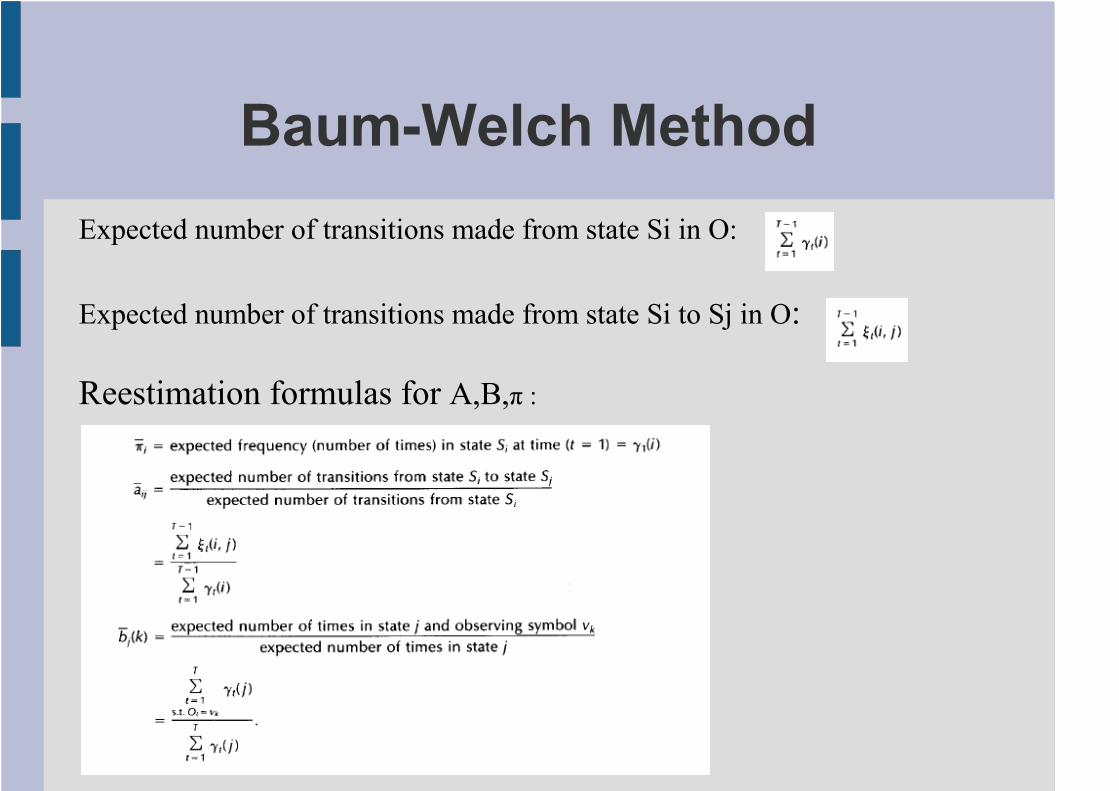
Expected number of transitions made from state Si in O:

Expected number of transitions made from state Si to Sj in O:

Reestimation formulas for A,B,π :

Baum-Welch Method

Current Model: λ (A,B,π)Reestimation Model: λ (A, B, π,)

Either;1) λ defines critical point of the likelihood function, where λ=λ2) model λ is more likely than λ

in the sense P(O|λ)>P(O|λ)

So λ is the new model matching the observation sequence better.

Using λ as λ iteratively and repeating reestimation calculation,improvement for the probability of O being observed in model is reached.Final result is called a maximum likelihood estimate of the HMM.

Baum-Welch Method

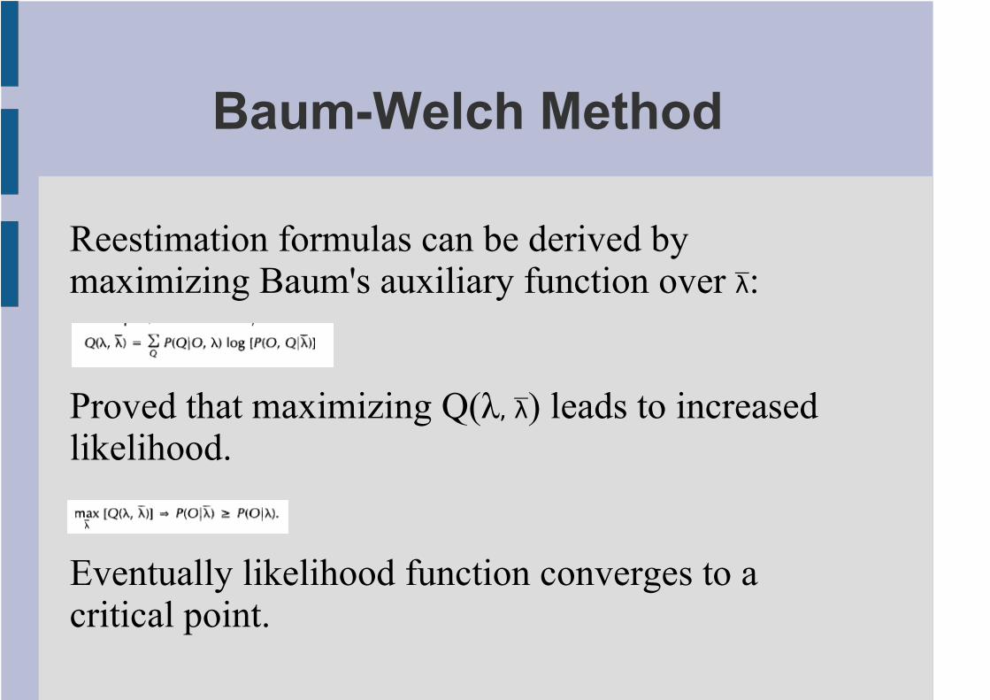
Reestimation formulas can be derived by maximizing Baum's auxiliary function over λ:

Proved that maximizing Q(λ, λ) leads to increased likelihood.

Eventually likelihood function converges to a critical point.

Baum-Welch Method

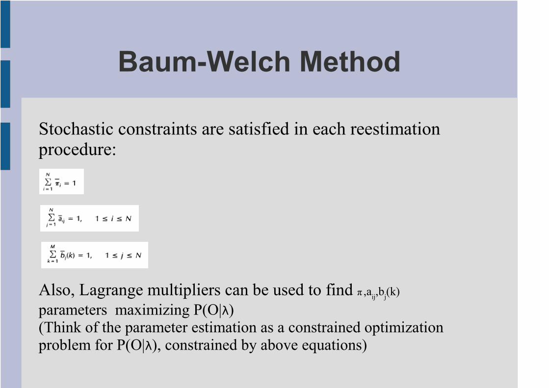
Stochastic constraints are satisfied in each reestimation procedure:

Also, Lagrange multipliers can be used to find π ,a

ij,b

j(k)

parameters maximizing P(O|λ)(Think of the parameter estimation as a constrained optimization problem for P(O|λ), constrained by above equations)

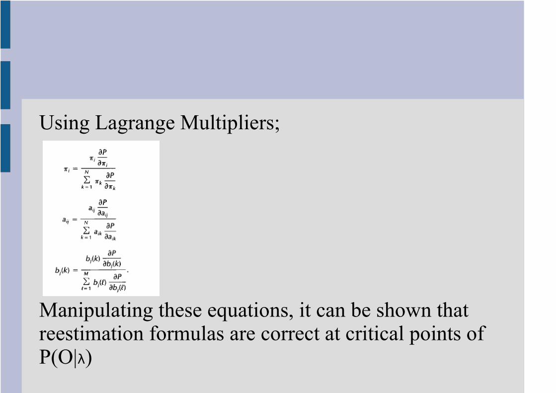
Using Lagrange Multipliers;

Manipulating these equations, it can be shown that reestimation formulas are correct at critical points of P(O|λ)

So far, considered only ergodic HMMs:Ergodic Model: Every state transition is possible. a

ij's positive.

Left-Right (Bakis) Model:As time increases, state index increases or stays the same. ie. states proceed from left to right.

Types of HMMs

Continuous Observation Densities in HMMs

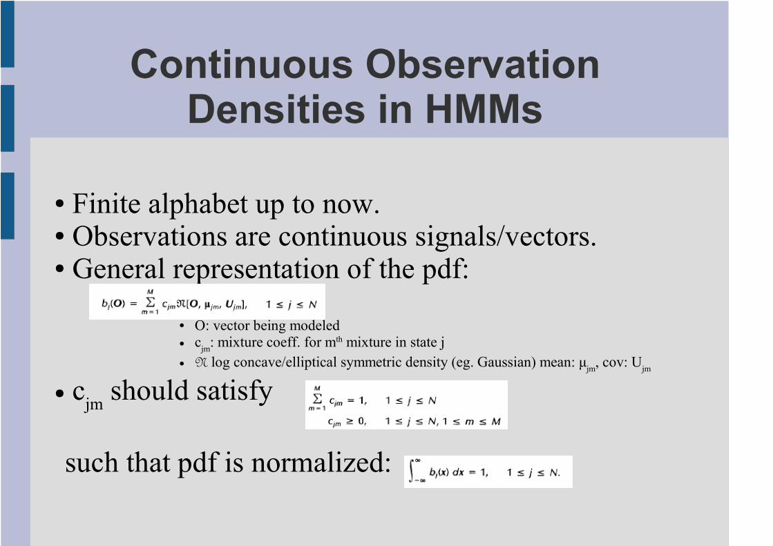
● Finite alphabet up to now.● Observations are continuous signals/vectors.● General representation of the pdf:

● O: vector being modeled● c

jm: mixture coeff. for mth mixture in state j

● N log concave/elliptical symmetric density (eg. Gaussian) mean: µjm

, cov: Ujm

● cjm

should satisfy

such that pdf is normalized:

Continuous Observation Densities in HMMs

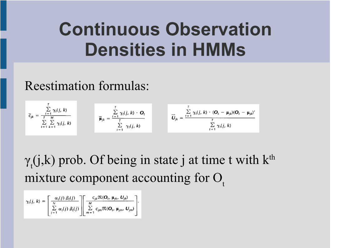
Reestimation formulas:

γt(j,k) prob. Of being in state j at time t with kth

mixture component accounting for Ot

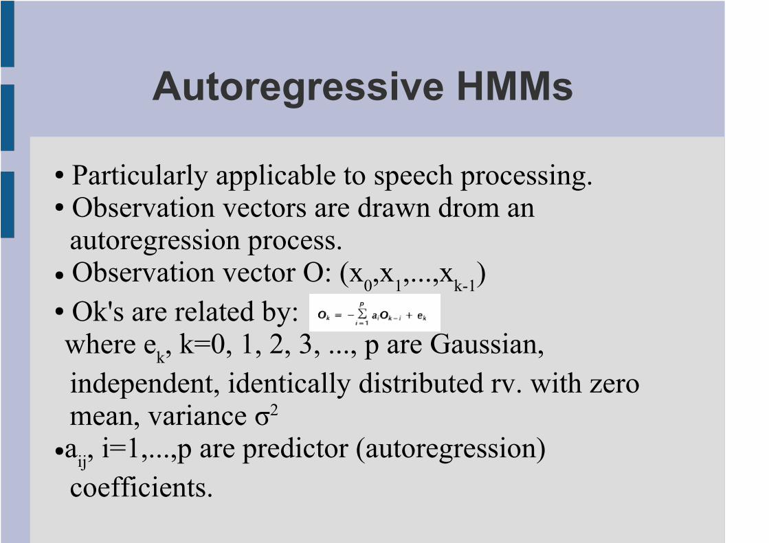
Autoregressive HMMs

● Particularly applicable to speech processing.● Observation vectors are drawn drom an

autoregression process.● Observation vector O: (x

0,x

1,...,x

k-1)

● Ok's are related by:where e

k, k=0, 1, 2, 3, ..., p are Gaussian,

independent, identically distributed rv. with zero mean, variance σ2

●aij, i=1,...,p are predictor (autoregression)

coefficients.

Autoregressive HMMs

● For large K, density function O is approximately:

where

● r(i) autocorrelation of observation samples● r

a(i) autocorr. Of autoreg. coeff.s

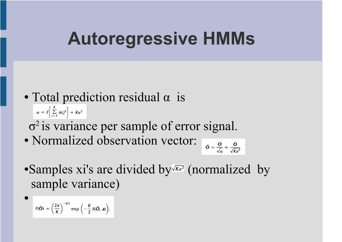
Autoregressive HMMs

● Total prediction residual α is

σ2 is variance per sample of error signal.● Normalized observation vector:

●Samples xi's are divided by (normalized by sample variance)

●

Autoregressive HMMs

Using Gaussian autoregressive density, assume the mixture density:

Each bjm

(O) is denstiy with autoregression vector ajm (or autocorr.vector rajm

)

Reestimation formula for sequence autocorrelation r(i) for the jth state, kth mixture component:

Where γt(j,k) is the prob. of being in state j at time t, using mixture component k,

Null Transitions

NULL Transitions:Observations are associated with the arcs of the model.Used for transitions which makes no output. (jumps between states produce no observation)Eg: a left-right model:

It is possible to omit transitions between states and conclude with 1 observation to account for a path beginning in state 1, ending in state N.

Tied States

●Equivalence relation between HMM parameters in different states.

●# of independent parameters in model is reduced.

●Used in cases where observation density is the same for two or more states. (eg in speech sounds)

●Model becomes simpler for parameter estimation

More...

● Inclusion of Explicit State Duration Density in HMMs

● Optimization Criterion

Bibliography

● A tutorial on Hidden Markov Models and Selected Applications in Speech Recognition,by Lawrence R. Rabiner

● Fundamentals of Speech Recognition,by Lawrence R. RabinerBiign Hwang Juang

Thanks for Listening!