hidden markov models - github pages · large margin hidden markov models for automatic speech...

Hidden Markov ModelsGabriela Tavares and Juri Minxha

Mentor: Taehwan KimCS159 04/25/2017

1

Outline1. Brief review of HMMs2. Hidden Markov Support Vector Machines3. Large Margin Hidden Markov Models for Automatic Speech Recognition4. Context-Dependent Pre-Trained Deep Neural Networks for

Large-Vocabulary Speech Recognition

2

Review of Hidden Markov Models

3

4

● A tool for representing probability distributions over sequences of observations

● A type of (dynamic) Bayesian network● Main assumptions: hidden states and Markov property

5

● a probability distribution over the initial state● the state transition matrix● the output model (emission matrix)

6

Learning in HMMs● Generative setting: model the joint distribution of inputs and outputs● Obtain the maximum likelihood estimate for the parameters of the HMM

given a set of output sequences● No tractable algorithm to solve this exactly● Baum-Welch (especial case of EM algorithm) can be used to obtain a local

maximum likelihood● Baum-Welch makes use of the forward-backward algorithm

7

Baum-Welch1. Initialize the model parameters: initial state distribution, transition and

emission matrices2. Compute the probability of being in state i at time t given an observed

sequence and the current estimate of the model parameters3. Compute the probability of being in state i and state j at times t and t+1,

respectively, given an observed sequence and the current estimate of the model parameters

4. Use these probabilities to update the estimate of the model parameters5. Repeat 2-4 iteratively until desired level of convergence

8

Forward-backward● Forward pass: recursively compute alpha(t), the joint probability of state

S(t) and the sequence of observations Y(1) to Y(t)

● Backward pass: compute beta(t), the conditional probabilities of the observations Y(t+1) to Y(T) given the state S(t)

● These probabilities are used to compute the expectations needed in Baum-Welch

9

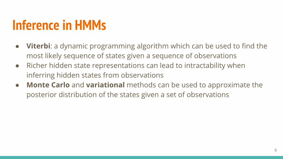
Inference in HMMs● Viterbi: a dynamic programming algorithm which can be used to find the

most likely sequence of states given a sequence of observations● Richer hidden state representations can lead to intractability when

inferring hidden states from observations● Monte Carlo and variational methods can be used to approximate the

posterior distribution of the states given a set of observations

Common applications of HMMs● Speech/phoneme recognition● Part-of-speech tagging● Computational molecular biology● Data compression● Vision: image sequence modelling, object tracking

10

HMM for POS Tagging

11

● Y = “Fish sleep”● S = (N, V)

● Y = “The dog ate my homework”● S = (D, N, V, D, N)

● Y = “The fox jumped over the fence”● S = (D, N, V, P, D, N)

HMM for Speech Recognition

12

13

Challenges and Limitations● HMMs model the joint distribution of states and observations; with a

(traditionally) generative learning procedure, we lose predictive power● Number of possible sequences grows exponentially with sequence length,

which is a challenge for large margin methods● The conditional independence assumption is too restrictive for many

applications● HMMs are based on explicit feature representations and lack the ability to

model nonlinear decision boundaries● HMMs cannot account for overlapping features

Hidden Markov Support Vector MachinesY Altun, I Tsochantaridis and T Hoffman (ICML 2003)

14

Quick Review of SVMs● Non-probabilistic binary linear

classifier● Find the hyperplane which maximizes

the margins● Samples on the margin are called

support vectors● Soft margins can be used (with slack

variables)● Nonlinear classification can be

achieved through the kernel trick (mapping inputs into high dimensional feature spaces)

15

Quick Review of SVMs

16

● Non-probabilistic binary linear classifier

● Find the hyperplane which maximizes the margins

● Samples on the margin are called support vectors

● Soft margins can be used (with slack variables)

● Nonlinear classification can be achieved through the kernel trick (mapping inputs into high dimensional feature spaces)

Limitations of Traditional HMMs● Typically trained in non-discriminative manner● Based on explicit feature representations and lack the power of

kernel-based methods● The conditional independence assumption is often too restrictive

17

Advantages of HM-SVMs● Discriminative approach to modeling● Can account for overlapping features (labels can depend directly on

features of past or future observations)● Maximum margin principle● Kernel-centric approach to learning nonlinear discriminant functions

Inherited from HMMs:

● Markov chain dependency structure between labels● Efficient dynamic programming formulation

18

Input-Output Mappings via Joint Feature Functions

Key idea: extract features not only from the input pattern (as in binary classification), but also jointly from input-output pairs

19

discriminant function

kernel trick

Hidden Markov Chain Discriminants

20

Problem description Feature representation


21

POS tagging example:

● denotes the input feature of “rain” occurring at position s

● encodes whether the word at t is a noun or not

● = 1 indicates the conjunction of these two predicates (a sequence where the word at s is “rain” and the word at t is a noun)

In HMMs, we use only and


22

Rewriting the inner product between feature vectors for different sequences:

The similarity between sequences depends on the number of common two-label fragments and on the inner product between the feature representation of patterns with common labels.

Structured Perceptron Learning

23

Hidden Markov Perceptron Learning

24

To avoid explicit evaluation of feature maps and direct representation of the discriminant function, we derive the dual of the perceptron algorithm:

Decompose F into two contributions:

Transition matrix

Emission matrixViterbi

Hidden Markov Perceptron Learning

25

“Perceptron-style” update

Viterbi decoding

We want to find the weight vector w which maximizes .

Hidden Markov SVM

26

Define the margin of a training example with respect to F:

Add constraint to prevent data points from falling into the margins:

We get an optimization problem with a quadratic objective:

Hidden Markov SVM

27

Replace each linear constraint with an equivalent set of linear constraints:

Rewrite constraints by introducing an additional threshold theta for every example:

Obtain dual formulation:

HM-SVM Optimization Algorithm

28

● Although we have a large set of possible label sequences, the actual solution might be extremely sparse (only a few negative pseudo-examples will become support vectors)

● We want to design an algorithm that exploits the anticipated sparseness of the solution

● Optimize W iteratively: at each iteration, optimize over the subspace spanned by all alpha_i(y) for a fixed i (i-th subspace)

● Use a working set approach to optimize over the i-th subspace, adding at most one negative pseudo-example to the working set at a time


29

Objective for the i-th subspace, to be maximized over the alpha_i while keeping all other alpha_j fixed:


30

Viterbi decoding

Initialize working set

Add negative pseudo-example to working set and optimize in the i-th subspace

Remove from the working set the sequences for which alpha_i is zero

Return current solution when constraint is broken

Soft Margin HM-SVM

● Use same working set approach from Algorithm 2, but with different constraints in the quadratic optimization (step 8)

31

Lagrangian:

● In the non-separable case, we can introduce slack variables to allow margin violations

32

Results for Named Entity Classification

33

Results for Part-of-Speech Tagging

Large Margin Hidden Markov Modelsfor Automatic Speech Recognition

F Sha and L K Saul (NIPS 2007)

34

What are we trying to do?● Infer correct hidden state sequence y = [y1,y2,...,yT] given observation

sequence X = [x1,x2,...,xT]● In automatic speech recognition (ASR), y can be words, phonemes, etc. In

this instance y is a set of 48 phonetic classes, each represented by a state in the HMM

● X is 39-dimensional real-valued acoustic feature vector (MFCCs)● Continuous density is needed to model emissions (we will use gaussian

mixture models)

35

GMMs for multiway classification

36

General form of mixture model

Gaussian mixture model

Learning Parameters for GMM

37

● Initialize parameters θ = {τ,μ1,μ2,Σ1,Σ2}

● Given current parameters, compute membership probability (i.e. soft clustering) for each data point (E-step)

● Adjust θ, such that it best explains the points assigned to each cluster (M-step)

Large Margin GMMs● In EM, we seek to maximize the joint likelihood of observed feature

vectors and label sequences● This however does not minimize phoneme or word error rates, which are

more relevant for automatic speech recognition● Unlike EM, we seek to maximize the distance between labeled examples● Decision rule for single ellipsoid (i.e. N(μi,Σi))

38

Large Margin GMMs● Decision rule for single ellipsoid (i.e. N(μi,Σi))

which can be reformulated as

39

Large Margin GMMs● Hard-margin maximization for single ellipsoid per class

40

Regularizes the scale of ellipsoidsEnforces margin condition

Restricts the matrix to be positive semidefinite

Large Margin GMMs

41

● Soft-margin (i.e. with slack variables)

● How does this margin maximization criteria generalize to case where each class is modeled as a mixture?

● Generate a “proxy label” for each data point (xn,yn,mn), where mn represents the mixture component label

42

Large Margin GMMs

● Reminder: HMM states are phonemes, observations are low-level spectral features of the recording

● Model emission densities with gaussian mixture models● Compute a score over a sequence of observations and states (note that

number of incorrect sequences grows as O(CT) )

● We can then define our margin constraints as

43

Sequential classification with CD-HMMs

Hamming Distance

● Number of constraints grows exponentially with the sequence length, there is 1 constraint for each incorrect sequence s

● Collapse the constraints

44


Softmax upper bound (why? differentiable with respect to model params)

i.e. log-likelihood of target sequence must be at least as good as next best one + handicap

● Full convex optimization problem:

45


Experiments

46

● Used TIMIT speech corpus for phonetic recognition● Error rate using hamming distance, compared to EM baseline● Utterance-based training is better than frame-based training

Context-Dependent Pre-Trained Deep Neural Networks for Large-Vocabulary Speech Recognition

G Dahl, D Yu, L Deng and A Acero (2012)

47

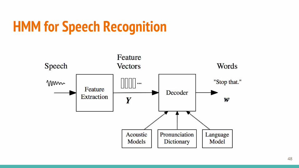
HMM for Speech Recognition

48

CD-DNN-HMM

49

● Key Concepts○ Context-dependent states in HMM○ Acoustic model as a deep belief network

■ Using restricted boltzmann machines○ Pre-training of deep neural network○ Deep neural network HMM hybrid acoustic model

Let’s have a look at what these things mean!

Context Dependence● Large vocabulary systems do not use words as units of sound

○ Vocabularies can consist of tens of thousands of words○ It’s difficult to find enough examples of every word even in large training datasets○ Words not seen in training cannot be learned

● Use sub-word units○ There are many more instances of sub-word units in a corpus than of words and

therefore HMM parameters can be better estimated○ Sub-word units can be combined to form new words○ Usually called phones

50

Context Dependence● Consider the word ROCK for example. Phonetically, we can write that as

R-AO-K● An HMM where states are context-independent phonemes is plausible● Phonemes are however very coarse units

○ When /AO/ is preceded by /R/ and followed by /K/, it has a different spectral signature than when it is preceded by /B/ and followed by /L/ as in the word ball

● We try to capture this variability, by considering phonemes in context

51

Context Dependence

52

● Number of triphones can be very large

● Realizing the amount of overlap between triphones, can we create a “codebook” by clustering triphone states that are similar?

● Each cluster called a senone● In the model under

consideration, these are the HMM states

CD-DNN-HMM

53



Joint probability over (v,h), where

Restricted Boltzmann Machines

54

● Undirected graphical model, where v = visible units (our data) and h = the hidden units b

c

Energy for (v,h) pair, where c and b are bias terms (for binary data)

Joint probability over (v,h), where


55

● Undirected graphical model, where v = visible units (our data) and h = the hidden units b

c

Energy for (v,h) pair, for real-valued feature vectors


56

● We can define a per-training-case log likelihood function as

● Where F(V) is known as the free energy and defined as

● In practice, gradient of log likelihood of data in RBM is hard to compute, so use MCMC methods (e.g. Gibbs sampling)

perform stochastic gradient descent on this


57

● Because there are no intra-layer connections, given v, we can easily infer the distribution over hidden units (and vice versa)

● This looks a lot like feedforward propagation in a neural network. Later this will allow us to use the weights of an RBM to initialize a feed-forward network.

CD-DNN-HMM

58



Pre-training a Deep Neural Network

59

● Stack a series of RBMs● Transfer learned weights to a

feedforward deep neural network and add softmax output layer

● Refine weights of DNN with labeled data

● Output of DNN are treated as “senones”

● Advantages: ○ Can use large set of

unsupervised data for pretraining, smaller one to further refine pre-trained DNN

○ Often achieves lower training error

○ Sort of data dependent regularization

MFCCs

CD-DNN-HMM

60



Model Architecture

61

● The decoded word sequence is determined as

where is the language model probability and the acoustic model is

Experimental Results● Bing mobile voice search application: ex. “Mcdonald's”,”Denny’s

restaurant”● Sampled at 8kHz● Collected under real usage scenarios, so contains all kinds of variations

such as noise, music, side-speech, accents, sloppy pronunciation● Language Model: 65K word unigrams, 3.2 million word bi-grams, and 1.5

million word trigrams● Sentence length is 2.1 tokens

62

Experimental Results● They computed sentence accuracy instead of word accuracy

○ Difficulties with word accuracy■ “Mc-Donalds”, “McDonalds”■ “Walmart”, “Wal-Mart”■ “7-eleven”, “7 eleven”, “seven-eleven”

○ Users only care if find the business or not, so the will repeat whole phrase if one if the words is not recognized

● Maximum 94% accuracy

63

Experimental Results● Baseline Systems

○ Performance of best CD-GMM-HMM summarized in table below

64

Maximum likelihoodMaximum mutual information

Minimum phone error

Experimental Results● Context independent vs. context dependent state labels

65

Experimental Results● Pre-training improves accuracy

66

Experimental Results● Accuracy as a function of the number of layers in DNN

67

Experimental Results● Training time

68

Experimental Results● Training time

○ So, to train a 5-layer CD-DNN-HMM, pre-training takes about(0.2 x 50) + (0.5 x 20) + (0.6 x 20) + (0.7 x 20) + (0.8 x 20) = 62 hours

○ Fine-tuning takes about 1.4 x 12 = 16.8 hours (for presented results 33.6 hours)

69

Experimental Results● Decoding time

70

Conclusions● CD-DNN-HMM performs better than its rival, the CD-GMM-HMM● It is however more computationally expensive● Bottlenecks

○ The bottleneck in the training process is the mini-batch stochastic gradient descent (SGD) algorithm.

○ Training in the study used the embedded Viterbi algorithm, which is not optimal for MFCCs

71

hidden markov models - github pages · large margin hidden markov models for automatic speech...

Documents