Seminar report On

Hidden Markov Model and Speech Recognition

by

Nirav S. Uchat

Roll No: 06305906

under the guidance of

Prof. Sivakumar

Department of Computer Science and Engineering

Indian Institute of Technology, Bombay

Mumbai

Contents

1 Introduction 1

2 Mathematical Understanding of Hidden Markov Model 22.1 Discrete Markov Process . . . . . . . . . . . . . . . . . . . . . . . . . . . . . . . . 22.2 Extension to Hidden Markov Model . . . . . . . . . . . . . . . . . . . . . . . . . 32.3 Elements Of Hidden Markov Model . . . . . . . . . . . . . . . . . . . . . . . . . . 42.4 The Three Basic Problem for HMMs . . . . . . . . . . . . . . . . . . . . . . . . . 62.5 Solution to Three Problem . . . . . . . . . . . . . . . . . . . . . . . . . . . . . . . 6

2.5.1 Forward Algorithm for Evaluation Problem [P (O|λ)] . . . . . . . . . . . . 72.5.2 Viterbi Algorithm for Decoding Hidden State Sequence P (Q,O|λ) . . . . 72.5.3 Baum-Welch Algorithm for Learning . . . . . . . . . . . . . . . . . . . . . 8

3 Speech Recognition and HMM 103.1 Block Diagram Of Speech Recognition . . . . . . . . . . . . . . . . . . . . . . . . 103.2 Vector quantization . . . . . . . . . . . . . . . . . . . . . . . . . . . . . . . . . . . 12

3.2.1 How to generate code book(K-means clustering algorithm) . . . . . . . . 133.2.2 Searching algorithm . . . . . . . . . . . . . . . . . . . . . . . . . . . . . . 13

3.3 Evaluation Problem and Viterbi Algorithm . . . . . . . . . . . . . . . . . . . . . 143.4 Language model . . . . . . . . . . . . . . . . . . . . . . . . . . . . . . . . . . . . 17

4 Isolated Word Recognizer 184.1 Architecture Of speech recognition . . . . . . . . . . . . . . . . . . . . . . . . . . 184.2 Example . . . . . . . . . . . . . . . . . . . . . . . . . . . . . . . . . . . . . . . . . 19

5 Conclusion and Future Work 22

i

Abstract

Modeling signal model for speech recognition is challenging task. It gives us great deal ofinformation about problem being modeled. In this seminar we will see how Hidden MarkovModel is used to model speech recognition application. We start with mathematical un-derstanding of HMM followed by problem faced by it and its solution. Then we move toblock diagram of speech recognition which include feature extraction, acoustic modeling andlanguage model, which works in tandem to generate search graph. Use of HMM in acousticmodeling is explained. At the end we will look at isolated word recognizer using HMM.

ii

1 Introduction

Real-world processes generally produce observable outputs which can be characterized as signals.The signals can be discrete in nature or continuous in nature. The signal source can be stationary(i.e., its statistical properties do not vary with time), or non-stationary (i.e., the signal propertiesvary over time). The signals can be pure or can be corrupted from other signal sources or bytransmission distortions.[2]

A problem of fundamental interest is characterizing such signal in terms of signal model,signal model gives us

• Theoretical description of a signal processing system which can be used toprocess the signal and so as to provide desired output.

• It helps up to understand great deal about signal source without having to havesource available.

One can classify signal model in to two types

• Deterministic Model : It exploit some known property of signal (like Amplitude of wave).

• Statistical Model : It takes statistical property of signal in to account. Example of thistype of model is Gaussian Model, Poisson Model, Markov Model and Hidden Markovmodel.

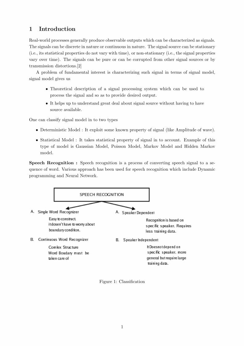
Speech Recognition : Speech recognition is a process of converting speech signal to a se-quence of word. Various approach has been used for speech recognition which include Dynamicprogramming and Neural Network.

Figure 1: Classification

1

In this seminar we will try to bridge speech recognition and HMM and figuring out howHMM can be effectively used in speech recognition problem.

Section 2 gives mathematical understanding of Hidden Markov Model. It also focuses onthree fundamental problems for HMM,namely:the probability of observation sequence given themodel i.e.,P (O/λ); the determination of single best state sequence, given the observation se-quence O = O1, O2, · · · , OT ; and the adjustment of model parameter λ = (A,B, π) to maximizerecognition probability. It also describe the method to efficiently solve this problems.

Section 3 explains block diagram of speech recognition system. We start with acoustic modeldesign using vector quantization which is used to convert feature vector to symbol. It also ex-plains how the algorithms described in 2nd section are used to solve the problem associatedwith speech recognition. This section discuss in detail about evaluation problem and viterbialgorithm for finding “single best” state sequence. Finally bi-gram language model is explained.

In Section 4, we will apply all technique discuss in previous section to understand the workingof isolated word recognizer.

2 Mathematical Understanding of Hidden Markov Model

Why Hidden Markov Model for Speech recognition ?

• HMM is very rich in mathematical structure and hence can form the theoretical basis foruse in a wide range of application.

• HMM model, when applied properly work well in practice for several important application.

2.1 Discrete Markov Process

Consider a system which may be described at any time as being in one of the state of set ofN distinct state, S1, S2, S3, · · · , SN ,. At regularly time interval system undergoes a change ofstate ( possibly back to same state) according to set of probability associated with the state.we denote time associated with state change as t =1,2 .., and we denote actual state at time tas qt. A full probabilistic description of above system, would in general require specification ofcurrent state and predecessor states. For the special case of discrete, first order , Markov chain,this probabilistic description is truncated to just current and the predecessor state i.e

P [qt = Sj |qt−1 = Si, qt−2 = Sk, · · ·] = P [qt = Sj |qt−1 = Si]

Furthermore we consider those processes in which the right hand side of above equation isindependent of time , thereby leading to the set of state transition probabilities aij of the form

aij = P [qt = Si|qt−1 = Sj ] 1 ≤ i, j ≤ N

with the state transition coefficients having the properties

aij ≥ 0N∑

j=1

aij = 1

2

The above process could be called as an observable Markov Model, since the output of theprocess is the set of states at each instant of time, where each state correspond to a observableevent.

2.2 Extension to Hidden Markov Model

In above model each state correspond to an observable event. This model is too restrictiveto be applicable to many problem of interest. we now extend this idea where observation isprobabilistic function of state. To get clear understanding we take coin tossing example.

Coin Toss Models: Assume the following scenario. You are in a room with a barrier throughwhich you cannot see what is happening. On the other side of the barrier is another personwho is performing a coin (or multiple coin) tossing experiment. The other person will not tellyou anything about what he is doing exactly, he will only tell you the result of each coin flip.Thus a sequence of hidden coin tossing experiments is performed, with the observation sequenceconsisting of a series of heads and tails, for e.g., a typical observation sequence would be

O = O1 O2 O3 · · ·OT (Head Tail Head · · ·Tail)

to model this coin tossing event with HMM, the fundamental question is

• What the state in model correspond to

• How many state in the model should there be

To understand this in better way lets take three different HMM

1. Single biased coin with two state - each state representing head or tail

2. Two biased coin with two state - each state representing single coin

3. Three biased coin with three state - with each coin representing single coin

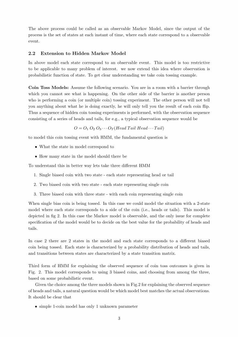
When single bias coin is being tossed. In this case we could model the situation with a 2-statemodel where each state corresponds to a side of the coin (i.e., heads or tails). This model isdepicted in fig 2. In this case the Markov model is observable, and the only issue for completespecification of the model would be to decide on the best value for the probability of heads andtails.

In case 2 there are 2 states in the model and each state corresponds to a different biasedcoin being tossed. Each state is characterized by a probability distribution of heads and tails,and transitions between states are characterized by a state transition matrix.

Third form of HMM for explaining the observed sequence of coin toss outcomes is given inFig. 2. This model corresponds to using 3 biased coins, and choosing from among the three,based on some probabilistic event.

Given the choice among the three models shown in Fig.2 for explaining the observed sequenceof heads and tails, a natural question would be which model best matches the actual observations.It should be clear that

• simple 1-coin model has only 1 unknown parameter

3

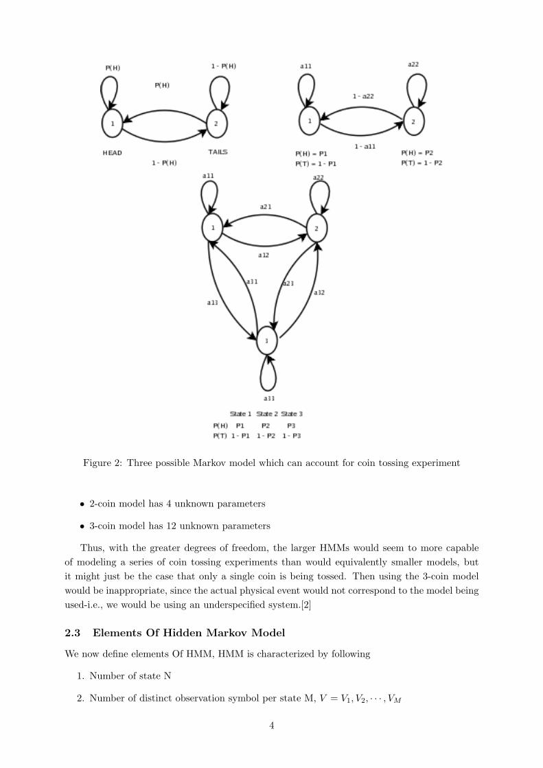
Figure 2: Three possible Markov model which can account for coin tossing experiment

• 2-coin model has 4 unknown parameters

• 3-coin model has 12 unknown parameters

Thus, with the greater degrees of freedom, the larger HMMs would seem to more capableof modeling a series of coin tossing experiments than would equivalently smaller models, butit might just be the case that only a single coin is being tossed. Then using the 3-coin modelwould be inappropriate, since the actual physical event would not correspond to the model beingused-i.e., we would be using an underspecified system.[2]

2.3 Elements Of Hidden Markov Model

We now define elements Of HMM, HMM is characterized by following

1. Number of state N

2. Number of distinct observation symbol per state M, V = V1, V2, · · · , VM

4

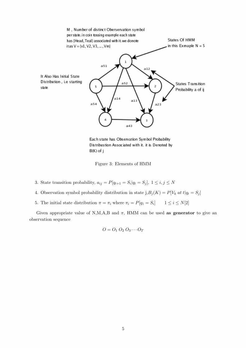
Figure 3: Elements of HMM

3. State transition probability, aij = P [qt+1 = Si|qt = Sj ], 1 ≤ i, j ≤ N

4. Observation symbol probability distribution in state j,Bj(K) = P [Vk at t|qt = Sj ]

5. The initial state distribution π = πi where πi = P [q1 = Si] 1 ≤ i ≤ N [2]

Given appropriate value of N,M,A,B and π, HMM can be used as generator to give anobservation sequence

O = O1 O2 O3 · · ·OT

5

2.4 The Three Basic Problem for HMMs

Problem 1 : Evaluation ProblemGiven the observation sequence O = O1 O2 · · · OT , and model λ = (A,B, π), how do weefficiently compute P (O|λ), the probability of observation sequence given the model.problem 1 is evaluation problem i.e given observation sequence and model, how do we computeprobability that observed sequence was produce by the model. we can think it as scoring problem.if you have to choose between many competing model then one with maximum probability willgive better result.

Figure 4: Evaluation Problem

Problem 2 : Hidden State Determination (Decoding)Given the observation sequence O = O1 O2 · · · OT , and model λ = (A,B, π), how do we choosecorresponding state sequence Q = q1 q2 · · · qT which is optimal in some meaningful sense.Problem 2 is one which attempts to uncover the hidden part of the problem. There is nocorrect solution to this problem, in practice we usually use optimal criterion to find best possiblesolution. For coin tossing example with observation sequence 0 = H H T T H correspondingstate sequence in each of the model (in Fig 2) can be

O = H H T T HModel 1 : S = 1 1 2 2 1Model 2 : S = 2 1 1 1 2Model 3 : S = 3 1 2 3 2

Problem 3 : LearningHow do we adjust the model parameter λ = (A,B, π) to maximize P (O|λ). Problem 3 is one inwhich we try to optimize model parameter so as to best describe as to how given observationsequence comes out. The observation sequence used here are called “training” sequence since itis used for training HMM. Training is one of the crucial element of HMM. It allows us to adjustmodel parameter as to create best model for given training sequence.[2]

2.5 Solution to Three Problem

Given this problem, it’s vital to solve them using efficient algorithm.

6

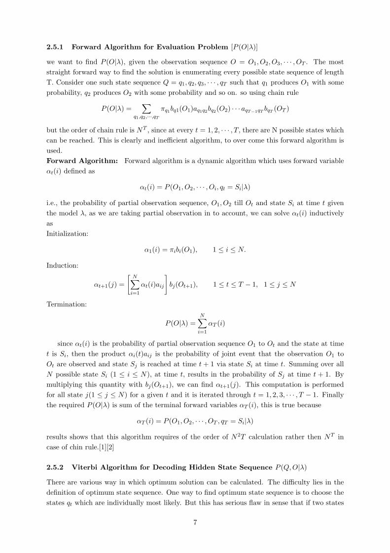
2.5.1 Forward Algorithm for Evaluation Problem [P (O|λ)]

we want to find P (O|λ), given the observation sequence O = O1, O2, O3, · · · , OT . The moststraight forward way to find the solution is enumerating every possible state sequence of lengthT. Consider one such state sequence Q = q1, q2, q3, · · · , qT such that q1 produces O1 with someprobability, q2 produces O2 with some probability and so on. so using chain rule

P (O|λ) =∑

q1,q2,···,qT

πq1bq1(O1)aq1q2bq2(O2) · · · aqT−1qT bqT (OT )

but the order of chain rule is NT , since at every t = 1, 2, · · · , T, there are N possible states whichcan be reached. This is clearly and inefficient algorithm, to over come this forward algorithm isused.Forward Algorithm: Forward algorithm is a dynamic algorithm which uses forward variableαt(i) defined as

αt(i) = P (O1, O2, · · · , Oi, qt = Si|λ)

i.e., the probability of partial observation sequence, O1, O2 till Ot and state Si at time t giventhe model λ, as we are taking partial observation in to account, we can solve αt(i) inductivelyasInitialization:

α1(i) = πibi(O1), 1 ≤ i ≤ N.

Induction:

αt+1(j) =

[N∑

i=1

αt(i)aij

]bj(Ot+1), 1 ≤ t ≤ T − 1, 1 ≤ j ≤ N

Termination:

P (O|λ) =N∑

i=1

αT (i)

since αt(i) is the probability of partial observation sequence O1 to Ot and the state at timet is Si, then the product αi(t)aij is the probability of joint event that the observation O1 toOt are observed and state Sj is reached at time t + 1 via state Si at time t. Summing over allN possible state Si (1 ≤ i ≤ N), at time t, results in the probability of Sj at time t + 1. Bymultiplying this quantity with bj(Ot+1), we can find αt+1(j). This computation is performedfor all state j(1 ≤ j ≤ N) for a given t and it is iterated through t = 1, 2, 3, · · · , T − 1. Finallythe required P (O|λ) is sum of the terminal forward variables αT (i), this is true because

αT (i) = P (O1, O2, · · · , OT , qT = Si|λ)

results shows that this algorithm requires of the order of N2T calculation rather then NT incase of chin rule.[1][2]

2.5.2 Viterbi Algorithm for Decoding Hidden State Sequence P (Q,O|λ)

There are various way in which optimum solution can be calculated. The difficulty lies in thedefinition of optimum state sequence. One way to find optimum state sequence is to choose thestates qt which are individually most likely. But this has serious flaw in sense that if two states

7

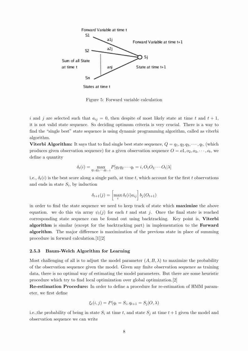
Figure 5: Forward variable calculation

i and j are selected such that aij = 0, then despite of most likely state at time t and t + 1,it is not valid state sequence. So deciding optimum criteria is very crucial. There is a way tofind the “single best” state sequence is using dynamic programming algorithm, called as viterbialgorithm.Viterbi Algorithm: It says that to find single best state sequence, Q = q1, q2.q3, · · · , qt, (whichproduces given observation sequence) for a given observation sequence O = o1, o2, o3, · · · , ot, wedefine a quantity

δt(i) = maxq1,q2,···,qt−1

P [q1q2 · · · qt = i, O1O2 · · ·Ot|λ]

i.e., δt(i) is the best score along a single path, at time t, which account for the first t observationsand ends in state Si, by induction

δt+1(j) =[max

iδt(i)aij

]bj(Ot+1)

in order to find the state sequence we need to keep track of state which maximize the aboveequation. we do this via array ψt(j) for each t and stat j. Once the final state is reachedcorresponding state sequence can be found out using backtracking. Key point is, Viterbialgorithm is similar (except for the backtracking part) in implementation to the Forwardalgorithm. The major difference is maximization of the previous state in place of summingprocedure in forward calculation.[1][2]

2.5.3 Baum-Welch Algorithm for Learning

Most challenging of all is to adjust the model parameter (A,B, λ) to maximize the probabilityof the observation sequence given the model. Given any finite observation sequence as trainingdata, there is no optimal way of estimating the model parameters. But there are some heuristicprocedure which try to find local optimization over global optimization.[2]Re-estimation Procedure: In order to define a procedure for re-estimation of HMM param-eter, we first define

ξt(i, j) = P (qt = Si, qt+1 = Sj |O, λ)

i.e.,the probability of being in state Si at time t, and state Sj at time t+ 1 given the model andobservation sequence we can write

8

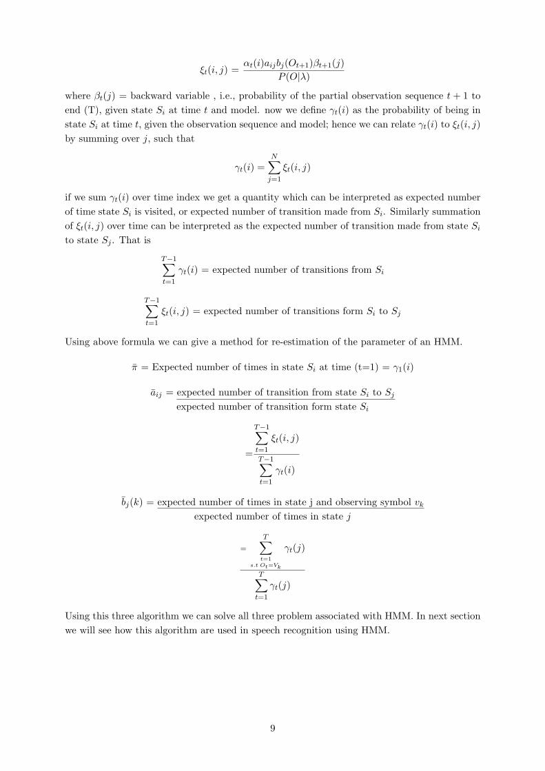
ξt(i, j) =αt(i)aijbj(Ot+1)βt+1(j)

P (O|λ)

where βt(j) = backward variable , i.e., probability of the partial observation sequence t + 1 toend (T), given state Si at time t and model. now we define γt(i) as the probability of being instate Si at time t, given the observation sequence and model; hence we can relate γt(i) to ξt(i, j)by summing over j, such that

γt(i) =N∑

j=1

ξt(i, j)

if we sum γt(i) over time index we get a quantity which can be interpreted as expected numberof time state Si is visited, or expected number of transition made from Si. Similarly summationof ξt(i, j) over time can be interpreted as the expected number of transition made from state Si

to state Sj . That is

T−1∑t=1

γt(i) = expected number of transitions from Si

T−1∑t=1

ξt(i, j) = expected number of transitions form Si to Sj

Using above formula we can give a method for re-estimation of the parameter of an HMM.

π = Expected number of times in state Si at time (t=1) = γ1(i)

aij = expected number of transition from state Si to Sj

expected number of transition form state Si

=

T−1∑t=1

ξt(i, j)

T−1∑t=1

γt(i)

bj(k) = expected number of times in state j and observing symbol vk

expected number of times in state j

=

T∑t=1

s.t Ot=Vk

γt(j)

T∑t=1

γt(j)

Using this three algorithm we can solve all three problem associated with HMM. In next sectionwe will see how this algorithm are used in speech recognition using HMM.

9

3 Speech Recognition and HMM

3.1 Block Diagram Of Speech Recognition

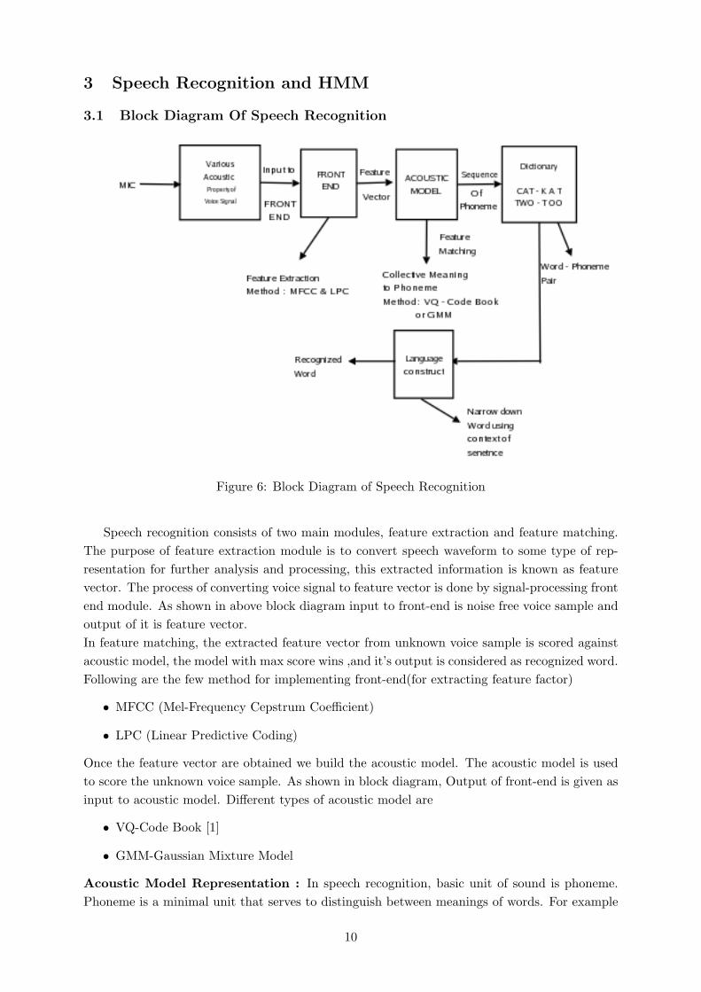
Figure 6: Block Diagram of Speech Recognition

Speech recognition consists of two main modules, feature extraction and feature matching.The purpose of feature extraction module is to convert speech waveform to some type of rep-resentation for further analysis and processing, this extracted information is known as featurevector. The process of converting voice signal to feature vector is done by signal-processing frontend module. As shown in above block diagram input to front-end is noise free voice sample andoutput of it is feature vector.In feature matching, the extracted feature vector from unknown voice sample is scored againstacoustic model, the model with max score wins ,and it’s output is considered as recognized word.Following are the few method for implementing front-end(for extracting feature factor)

• MFCC (Mel-Frequency Cepstrum Coefficient)

• LPC (Linear Predictive Coding)

Once the feature vector are obtained we build the acoustic model. The acoustic model is usedto score the unknown voice sample. As shown in block diagram, Output of front-end is given asinput to acoustic model. Different types of acoustic model are

• VQ-Code Book [1]

• GMM-Gaussian Mixture Model

Acoustic Model Representation : In speech recognition, basic unit of sound is phoneme.Phoneme is a minimal unit that serves to distinguish between meanings of words. For example

10

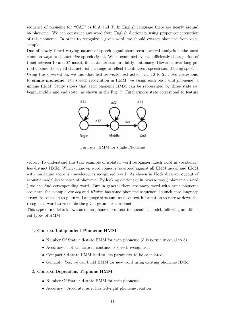
sequence of phoneme for “CAT” is K A and T. In English language there are nearly around46 phoneme. We can construct any word from English dictionary using proper concatenationof this phoneme. In order to recognize a given word, we should extract phoneme from voicesample.Due of slowly timed varying nature of speech signal short-term spectral analysis is the mostcommon ways to characterize speech signal. When examined over a sufficiently short period oftime(between 10 and 25 msec), its characteristics are fairly stationary. However, over long pe-riod of time the signal characteristic change to reflect the different speech sound being spoken.Using this observation, we find that feature vector extracted over 10 to 25 msec correspondto single phoneme. For speech recognition in HMM, we assign each basic unit(phoneme) aunique HMM. Study shows that each phoneme HMM can be represented by three state i.e.begin, middle and end state. as shown in the Fig. 7. Furthermore state correspond to feature

Figure 7: HMM for single Phoneme

vector. To understand this take example of isolated word recognizer, Each word in vocabularyhas distinct HMM. When unknown word comes, it is scored against all HMM model and HMMwith maximum score is considered as recognized word. As shown in block diagram output ofacoustic model is sequence of phoneme. By looking dictionary in reverse way ( phoneme - word) we can find corresponding word. But in general there are many word with same phonemesequence, for example car key and Khakee has same phoneme sequence. In such case languagestructure comes in to picture. Language structure uses context information to narrow down therecognized word to resemble the given grammar construct.This type of model is known as mono-phone or context-independent model, following are differ-ent types of HMM

1. Context-Independent Phoneme HMM

• Number Of State : d-state HMM for each phoneme (d is normally equal to 3)

• Accuracy : not accurate in continuous speech recognition

• Compact : d-state HMM lead to less parameter to be calculated

• General : Yes, we can build HMM for new word using existing phoneme HMM

2. Context-Dependent Triphone HMM

• Number Of State : d-state HMM for each phoneme

• Accuracy : Accurate, as it has left-right phoneme relation

11

• Compact : Each phoneme has immediate left-right relation, more parameter needsto be calculated

• General : Yes

3. Whole-Word HMM

• Number Of state : No phoneme generation

• assign number of state to model a word as whole

• Accurate : Yes, require large training data and work for small vocabulary

• Compact : No, need too many state as vocabulary increases

• General : No, can’t build new word using this representation

In practice triphone model is widely used in speech recognition using Hidden Markov Model.Now we are not going to discuss how feature vector are extracted from voice signal. we assumethat using either MFCC or LPC we get required feature vector. In case of MFCC it is 39dimension vector. The question is how to map feature vector to HMM state ?for doing so we use technique called Vector Quantization.

3.2 Vector quantization

It is a technique for mapping MFCC type feature vector to symbol.

• create training set of feature vector

• cluster them in to small number of classes

• represent each class by symbol

• for each class Vk, compute the probability that it is generated by given HMM state.

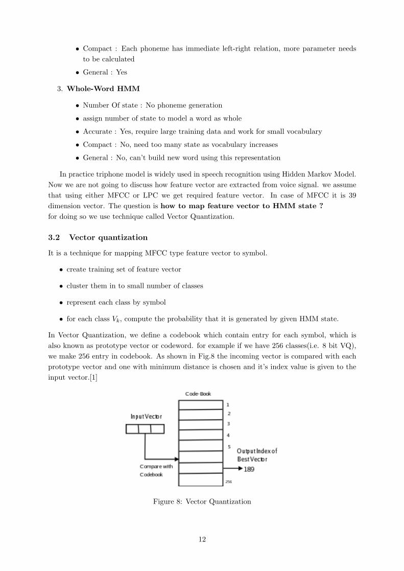
In Vector Quantization, we define a codebook which contain entry for each symbol, which isalso known as prototype vector or codeword. for example if we have 256 classes(i.e. 8 bit VQ),we make 256 entry in codebook. As shown in Fig.8 the incoming vector is compared with eachprototype vector and one with minimum distance is chosen and it’s index value is given to theinput vector.[1]

Figure 8: Vector Quantization

12

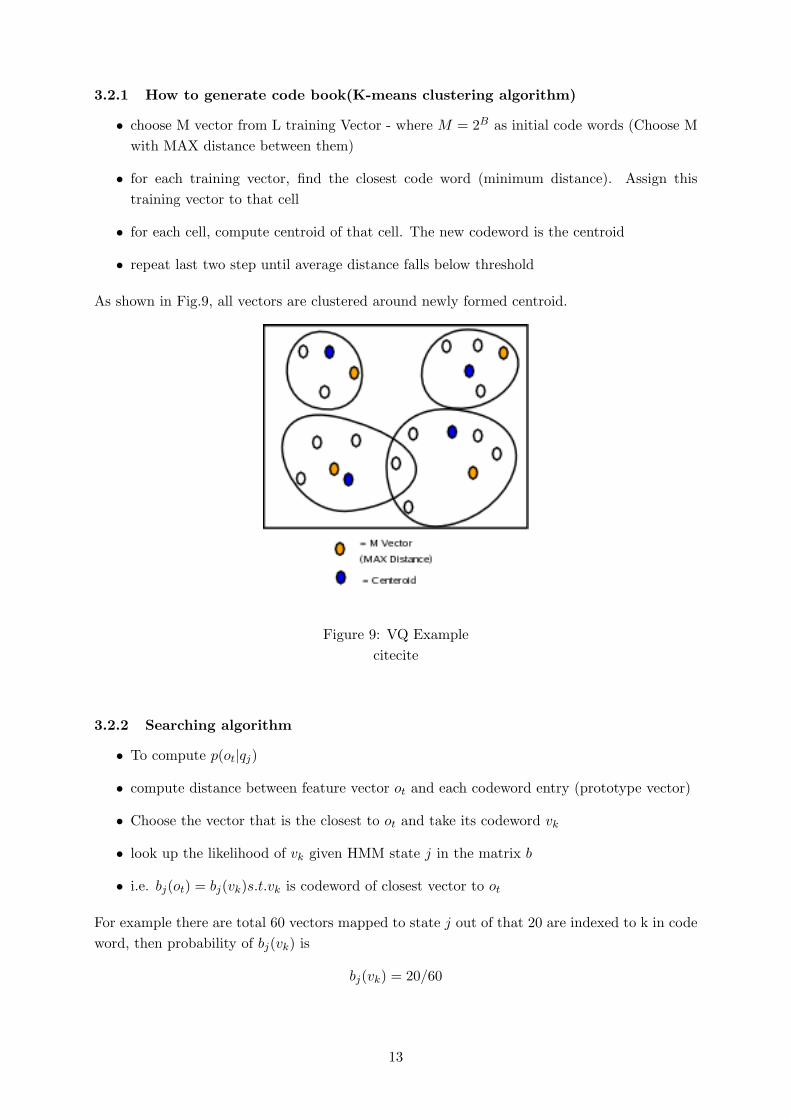
3.2.1 How to generate code book(K-means clustering algorithm)

• choose M vector from L training Vector - where M = 2B as initial code words (Choose Mwith MAX distance between them)

• for each training vector, find the closest code word (minimum distance). Assign thistraining vector to that cell

• for each cell, compute centroid of that cell. The new codeword is the centroid

• repeat last two step until average distance falls below threshold

As shown in Fig.9, all vectors are clustered around newly formed centroid.

Figure 9: VQ Examplecitecite

3.2.2 Searching algorithm

• To compute p(ot|qj)

• compute distance between feature vector ot and each codeword entry (prototype vector)

• Choose the vector that is the closest to ot and take its codeword vk

• look up the likelihood of vk given HMM state j in the matrix b

• i.e. bj(ot) = bj(vk)s.t.vk is codeword of closest vector to ot

For example there are total 60 vectors mapped to state j out of that 20 are indexed to k in codeword, then probability of bj(vk) is

bj(vk) = 20/60

13

3.3 Evaluation Problem and Viterbi Algorithm

In Section 2 we saw evaluation problem i.e., given observation sequence O = O1, O2, O3, · · · , OT

how to calculate P (O|λ). There we apply chain rule for calculating P (O|λ) as

Figure 10: chain rule - intractable algorithm

P (O|λ) =∑

overallstate

πq1bq1(O1)aq1q2bq2(O2) · · · aqT−1qT bqT (OT )

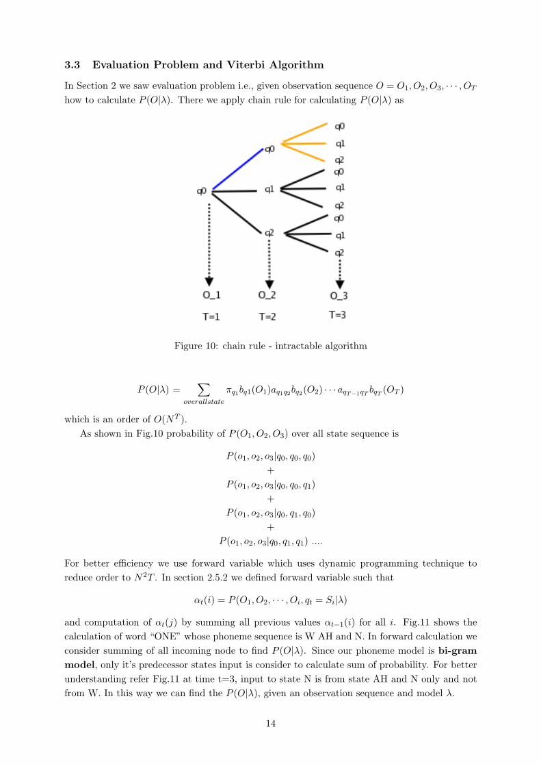
which is an order of O(NT ).As shown in Fig.10 probability of P (O1, O2, O3) over all state sequence is

P (o1, o2, o3|q0, q0, q0)+

P (o1, o2, o3|q0, q0, q1)+

P (o1, o2, o3|q0, q1, q0)+

P (o1, o2, o3|q0, q1, q1) ....

For better efficiency we use forward variable which uses dynamic programming technique toreduce order to N2T . In section 2.5.2 we defined forward variable such that

αt(i) = P (O1, O2, · · · , Oi, qt = Si|λ)

and computation of αt(j) by summing all previous values αt−1(i) for all i. Fig.11 shows thecalculation of word “ONE” whose phoneme sequence is W AH and N. In forward calculation weconsider summing of all incoming node to find P (O|λ). Since our phoneme model is bi-grammodel, only it’s predecessor states input is consider to calculate sum of probability. For betterunderstanding refer Fig.11 at time t=3, input to state N is from state AH and N only and notfrom W. In this way we can find the P (O|λ), given an observation sequence and model λ.

14

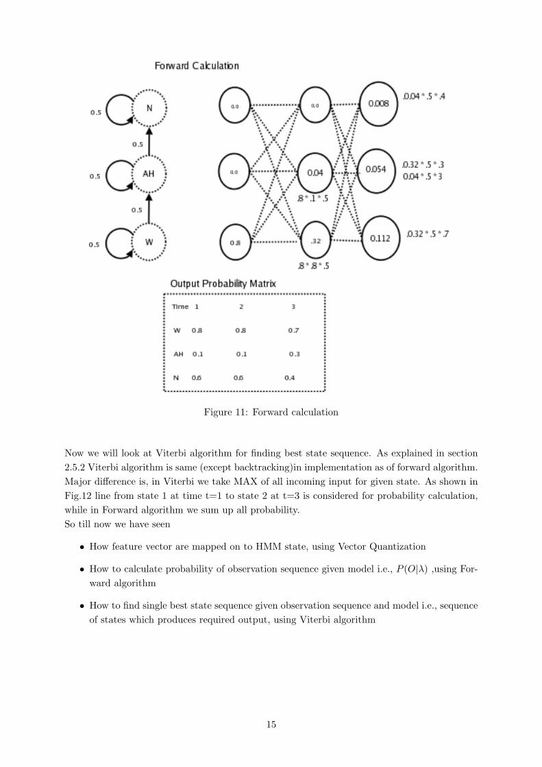
Figure 11: Forward calculation

Now we will look at Viterbi algorithm for finding best state sequence. As explained in section2.5.2 Viterbi algorithm is same (except backtracking)in implementation as of forward algorithm.Major difference is, in Viterbi we take MAX of all incoming input for given state. As shown inFig.12 line from state 1 at time t=1 to state 2 at t=3 is considered for probability calculation,while in Forward algorithm we sum up all probability.So till now we have seen

• How feature vector are mapped on to HMM state, using Vector Quantization

• How to calculate probability of observation sequence given model i.e., P (O|λ) ,using For-ward algorithm

• How to find single best state sequence given observation sequence and model i.e., sequenceof states which produces required output, using Viterbi algorithm

15

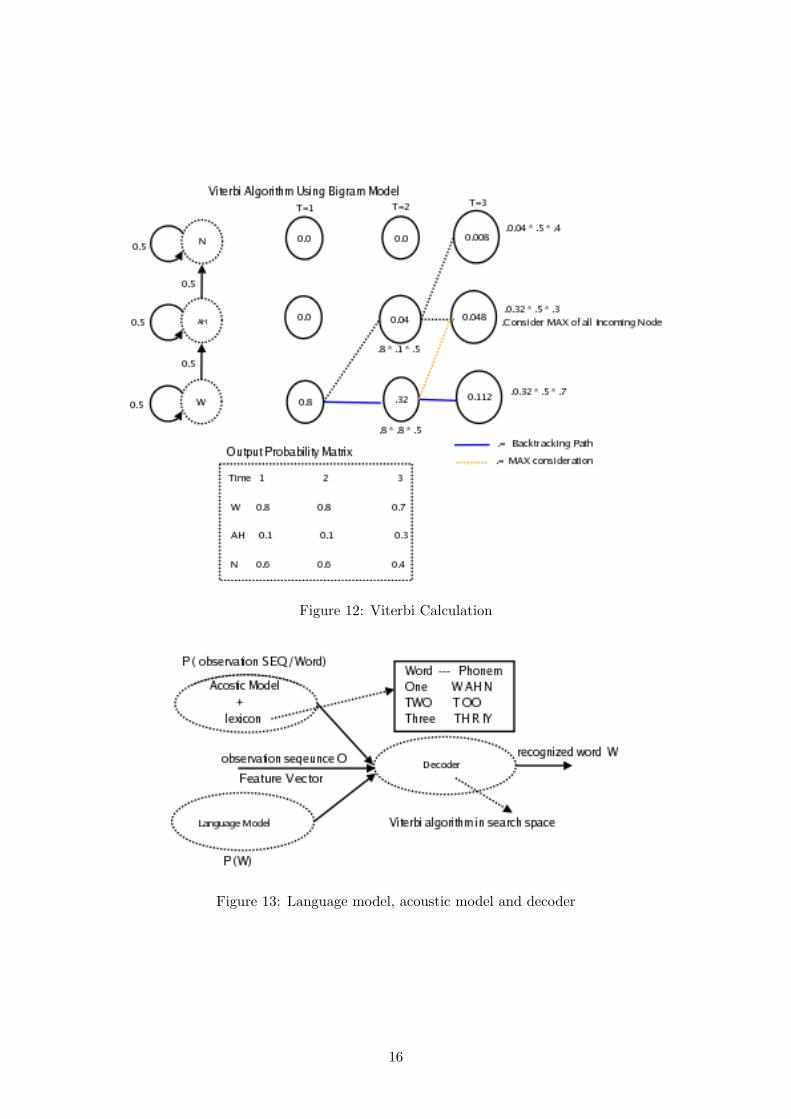
Figure 12: Viterbi Calculation

Figure 13: Language model, acoustic model and decoder

16

3.4 Language model

The model that compute P (W ) is known as Language model. Fig.13 gives how Acoustic model,Decoder and Language model work together to recognize given sentence/word W . Given asentence how one can calculate the joint probability. One way is to use chain rule. In generalP (A,B,C,D) = P (A).P (B|A).P (C|A,B).P (D|A,B,C). For an example what is the probabil-ity of P(computer,got,crashed,while,installing,windows). Using above rule we can write

P(computer)* P(got/computer)* P(crashed/computer,got)* P(while/computer,got,crashed)*P(installing/computer,got,crashed,while)* P(windows/computer,got,crashed,while,installing)

In practice we will never get data to calculate the probability of long prefix such asP(windows/computer,got,crashed,while,installing)In order to model practical application we can make assumption of calculating P(got/computer),P(crashed/got), P(windows/installing) and so on. This is known as bi-gram model. In generalwe write,

P (Wn|Wn−1)

Language model help us in generating search graph. Search graph is collection of HMM of eachphoneme in given vocabulary. Once the graph is created, incoming feature vector are quantizedand search is performed to find best sequence of phoneme. Fig.14 will give better understandingof search graph.

Figure 14: Search graph for given vocabulary

17

4 Isolated Word Recognizer

In this section we will quickly go through all the components used in speech recognition appli-cation.

4.1 Architecture Of speech recognition

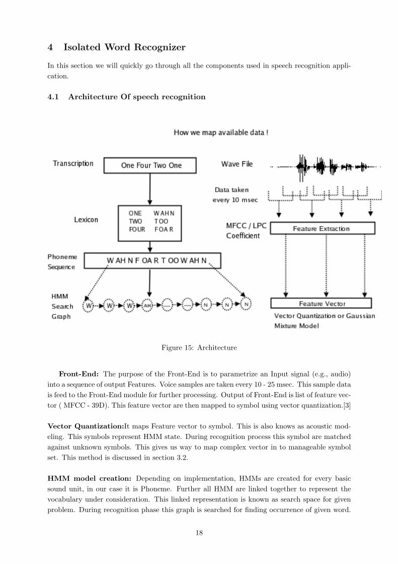
Figure 15: Architecture

Front-End: The purpose of the Front-End is to parametrize an Input signal (e.g., audio)into a sequence of output Features. Voice samples are taken every 10 - 25 msec. This sample datais feed to the Front-End module for further processing. Output of Front-End is list of feature vec-tor ( MFCC - 39D). This feature vector are then mapped to symbol using vector quantization.[3]

Vector Quantization:It maps Feature vector to symbol. This is also knows as acoustic mod-eling. This symbols represent HMM state. During recognition process this symbol are matchedagainst unknown symbols. This gives us way to map complex vector in to manageable symbolset. This method is discussed in section 3.2.

HMM model creation: Depending on implementation, HMMs are created for every basicsound unit, in our case it is Phoneme. Further all HMM are linked together to represent thevocabulary under consideration. This linked representation is known as search space for givenproblem. During recognition phase this graph is searched for finding occurrence of given word.

18

To represent relation between the words in given sentence, bi-gram model is used. Languagemodel, vocabulary and acoustic modeling forms the core of speech recognition. Lexicon (Fig.13)are used to map word from vocabulary to HMM. For example consider word ”ONE”, in lexiconlisting we have it’s corresponding phoneme sequence.

Training: The most difficult task is to adjust the model parameter to accurately representthe word under consideration. In training mode large amount of voice data ( from differentspeaker ) is given to HMM model. Using this, HMM adjust its probability distribution andtransition matrix. There is no global optimal algorithm for learning. Every HMM must betrained to maximize it’s (local optimum) recognition power. Initially HMM for phoneme (beforelearning) consists of 3-state and it’s adjacency matrix and output probability distribution areinitialized randomly. It gets automatically updated once the training starts.[4]

Recognition : unknown word is fed to HMM and it’s output probability is calculated.

Five steps for automatic speech recognition(ASR)

• Feature Extraction: 39 MFCC features

• Acoustic Model: Vector Quantization - Output probability distribution for each state

• Lexicon: Word to Phoneme mapping - Used in creation of HMM

• Language Model: N-grams for computing P (wi|wi−1)

• Decoder: Viterbi algorithm, using dynamic programming for combining all these to getword sequence from speech!

4.2 Example

The role of the recognizer is to do mapping between sequences of speech vectors and the wantedunderlying symbol sequences. Two problems make this very difficult

• The mapping from symbols to speech is not one-to-one since different underlying symbolscan give rise to similar speech sounds(example of car key and khakee having same phonemesequence). Furthermore, there are large variations in the speech waveform due to speakervariability, noise, environment, etc.

• The boundaries between symbols cannot be identified explicitly from the speech waveform.Hence, it is not possible to treat the speech waveform as a sequence of concatenatedpatterns.

The second problem of not knowing the word boundary locations can be avoided by restrictingthe task to Isolated word recognition (Fig.16). In this the speech waveform corresponds toa single word chosen from a fixed vocabulary. Despite it is very artificial, it has wide range ofpractical applications. It serves as basic model to understand the concept of speech recognition.

We Assume that parameter aij and bj(ot) are known for each model Mi. Given a set ofexample for a given word, HMM model parameter can be calculated automatically using learn-ing algorithm discussed in section 2.5.3. Fig 17 summarize the use of HMM in isolated word

19

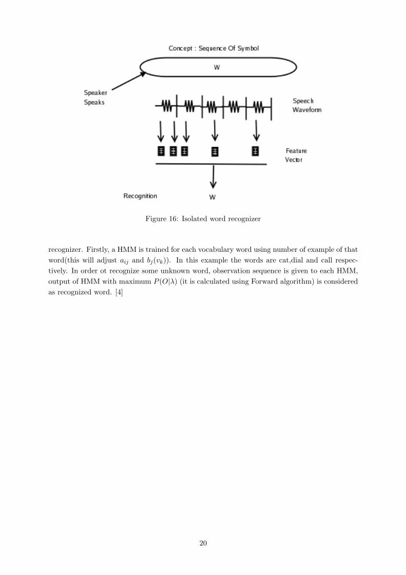
Figure 16: Isolated word recognizer

recognizer. Firstly, a HMM is trained for each vocabulary word using number of example of thatword(this will adjust aij and bj(vk)). In this example the words are cat,dial and call respec-tively. In order ot recognize some unknown word, observation sequence is given to each HMM,output of HMM with maximum P (O|λ) (it is calculated using Forward algorithm) is consideredas recognized word. [4]

20

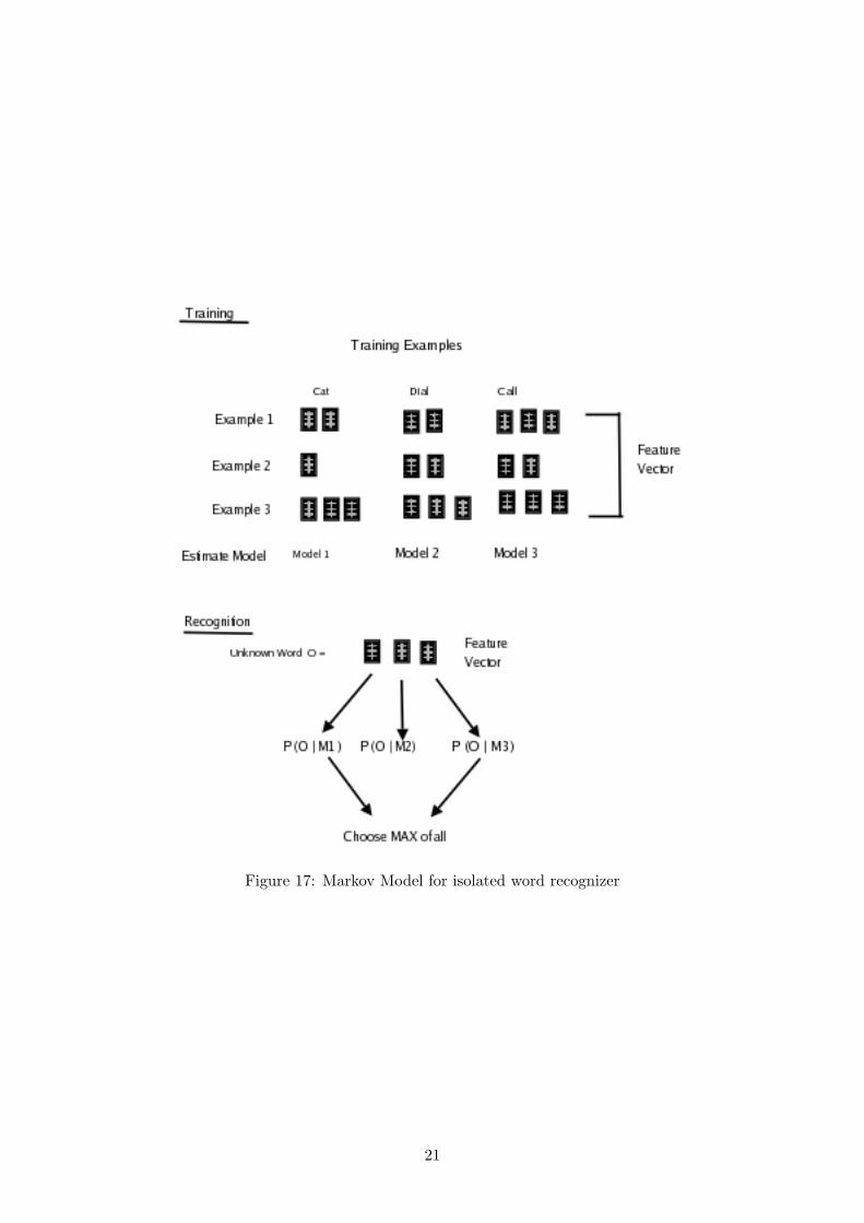
Figure 17: Markov Model for isolated word recognizer

21

5 Conclusion and Future Work

We saw how HMM can be used as signal model for speech recognition application. Forward,Viterbi and Baum-Welch algorithm provide solution to three problem associated with HMM.Speech recognition using HMM gives good result due to resemblance between architecture ofHMM and varying speech data. Neural Network is another method, which uses gradient decentmethod with back propagation algorithm. Study shows that this method works well in presenceof large amount of training data also the recognition accuracy is high if the word under consid-eration is from training data set. While in HMM, the recognition ability is good for unknownword. HMM is generic concept and is used in many area of research.

In whole architecture of speech recognition, HMM is just one block which help in creatingsearch graph. It work in tandem with other block such as front-end, language model, lexicon toachieve desired goal. The purpose of HMM is to map feature vector to some representable stateand emit symbol, concatenation of which gives desired phoneme sequence.

Problem with continuous speech recognition is, to determine word boundary. It requiresknowledge of language construct and regional accent understanding. Other problem is presenceof noise in sample data. Efficient solution to this two problem is required for accurate continuousspeech recognition.

What we discussed in this seminar is recognition of English sentence, we can extend thismodel to recognize multi-lingual sentence.

22

References

[1] Dan Jurafsky. CS 224S / LINGUIST 181 Speech Recognition and Synthesis. World WideWeb, http://www.stanford.edu/class/cs224s/.

[2] Lawrence R. Rabiner. A Tutorial on Hidden Markov Model and Selected Applicaiton inSpeech Recognition. IEEE, 1989.

[3] Willie Walker, Paul Lamere, and Philip Kwok. Sphinx-4: A Flexible Open Source Frameworkfor Speech Recognition. SUN Microsystem, 2004.

[4] Steve Young and Gunnar Evermannl. The HTK Book. Microsoft Corporation, 2005.

23