1

HIDDEN MARKOV MODELSIN SPEECH RECOGNITION

Wayne Ward

Carnegie Mellon University

Pittsburgh, PA

2

Acknowledgements

Much of this talk is derived from the paper

"An Introduction to Hidden Markov Models",

by Rabiner and Juang

and from the talk

"Hidden Markov Models: Continuous SpeechRecognition"

by Kai-Fu Lee

3

Topics

• Markov Models and Hidden Markov Models

• HMMs applied to speech recognition

• Training

• Decoding

4

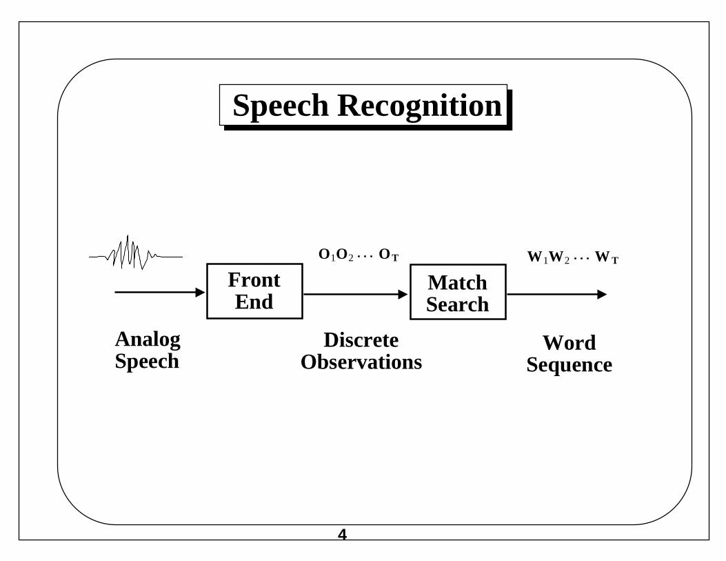
Speech Recognition

FrontEnd

MatchSearch

O1O2 OT

AnalogSpeech

DiscreteObservations

W1W2 W T

WordSequence

5

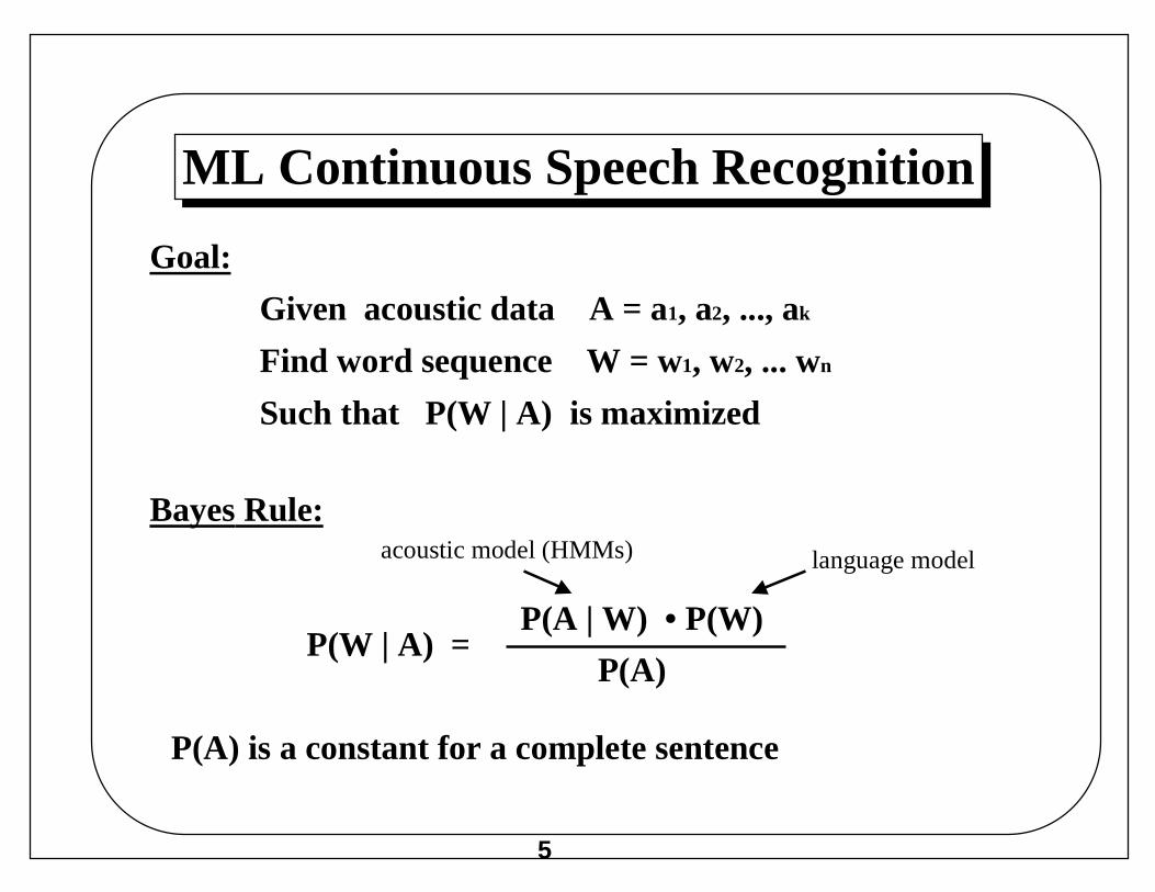
ML Continuous Speech Recognition

Goal:

Given acoustic data A = a1, a2, ..., ak

Find word sequence W = w1, w2, ... wn

Such that P(W | A) is maximized

P(W | A) = P(A | W) • P(W)

P(A)

acoustic model (HMMs) language model

Bayes Rule:

P(A) is a constant for a complete sentence

6

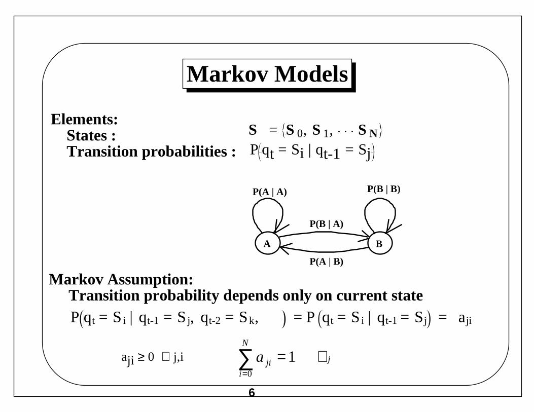
Markov Models

Elements: States : Transition probabilities :

Markov Assumption: Transition probability depends only on current state

S = S 0, S 1, S N

P(A | A) P(B | B)

P(B | A)

P(A | B)

A B

P qt = Si | qt-1 = Sj, qt-2 = Sk, = P qt = Si | qt-1 = Sj = aji

aji ≥ 0 ∀ j,i

P qt = Si | qt-1 = Sj

j

N

ijia ∀=∑

=

10

7

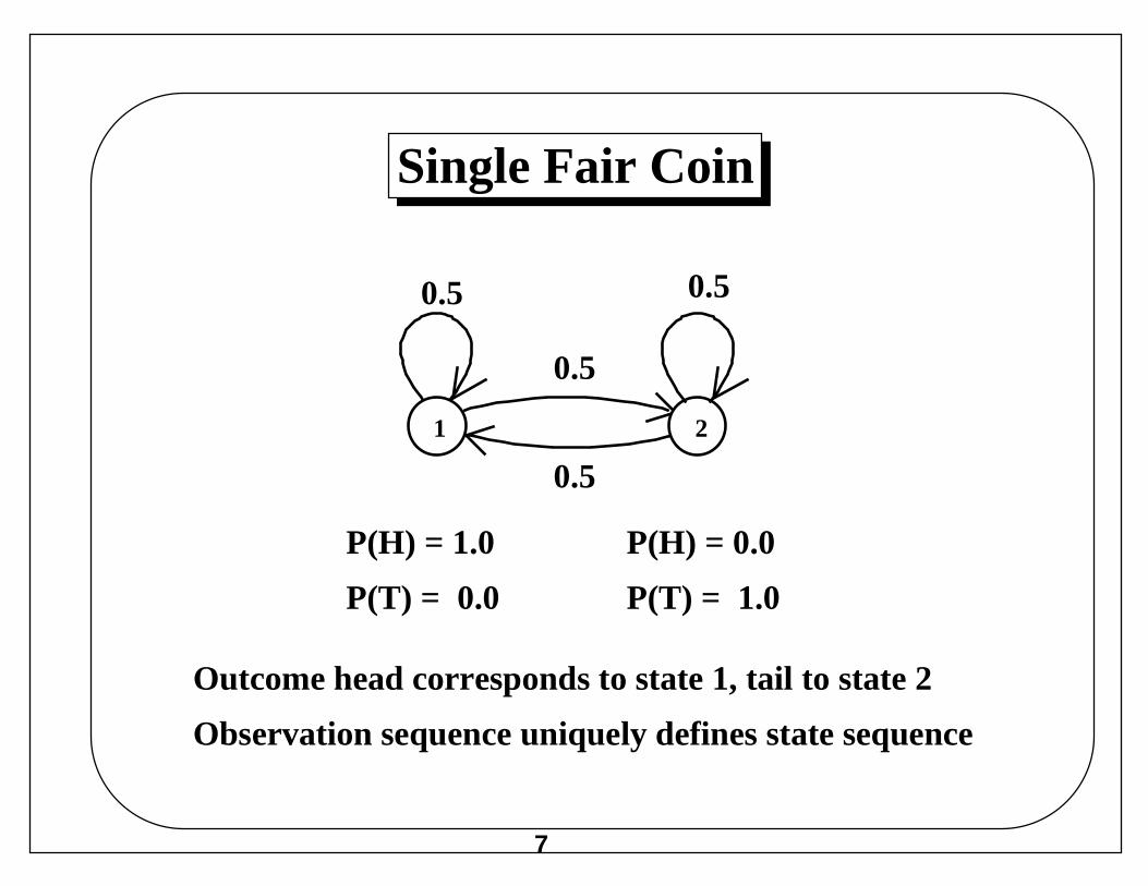
Single Fair Coin

0.5 0.5

0.5

0.5

1 2

P(H) = 1.0

P(T) = 0.0

P(H) = 0.0

P(T) = 1.0

Outcome head corresponds to state 1, tail to state 2

Observation sequence uniquely defines state sequence

8

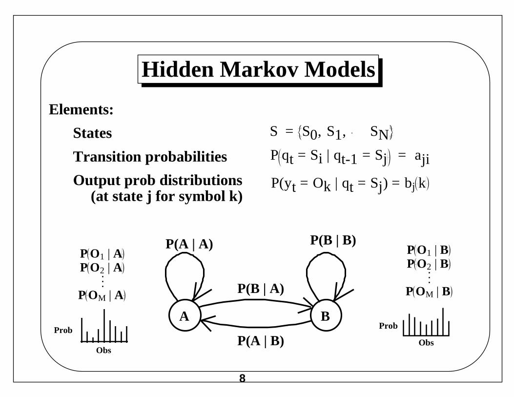
Hidden Markov Models

P(A | A) P(B | B)

P(B | A)

P(A | B)

A B

Obs

ProbProb

Obs

P O1 | BP O2 | B

P OM | B

P O1 | AP O2 | A

P OM | A

S = S0, S1, SN P qt = Si | qt-1 = Sj = aji

Elements:

States

Transition probabilities

Output prob distributions(at state j for symbol k)

P(yt = Ok | qt = Sj) = bj k

9

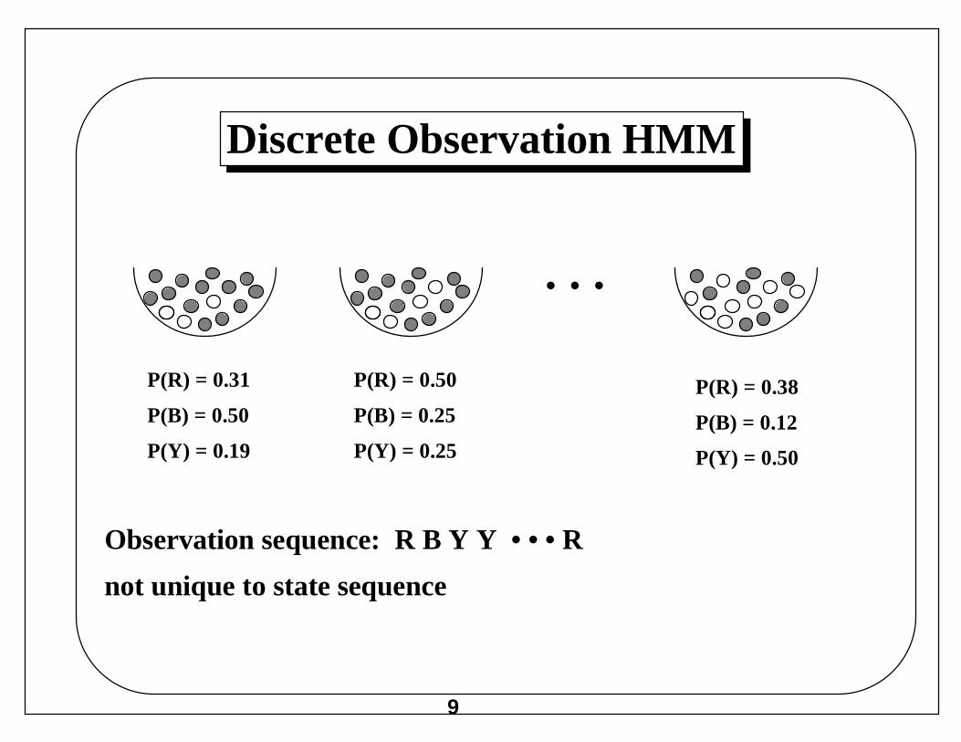
Discrete Observation HMM

P(R) = 0.31

P(B) = 0.50

P(Y) = 0.19

P(R) = 0.50

P(B) = 0.25

P(Y) = 0.25

P(R) = 0.38

P(B) = 0.12

P(Y) = 0.50

• • •

Observation sequence: R B Y Y • • • R

not unique to state sequence

10

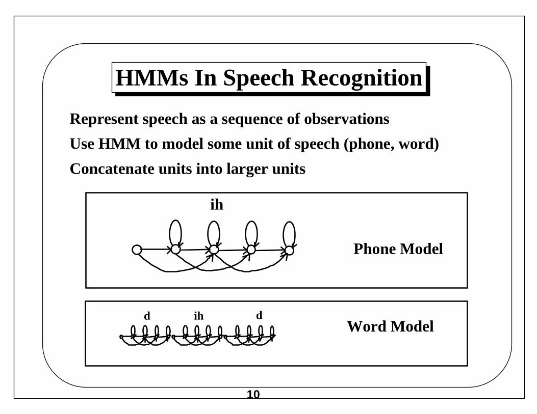
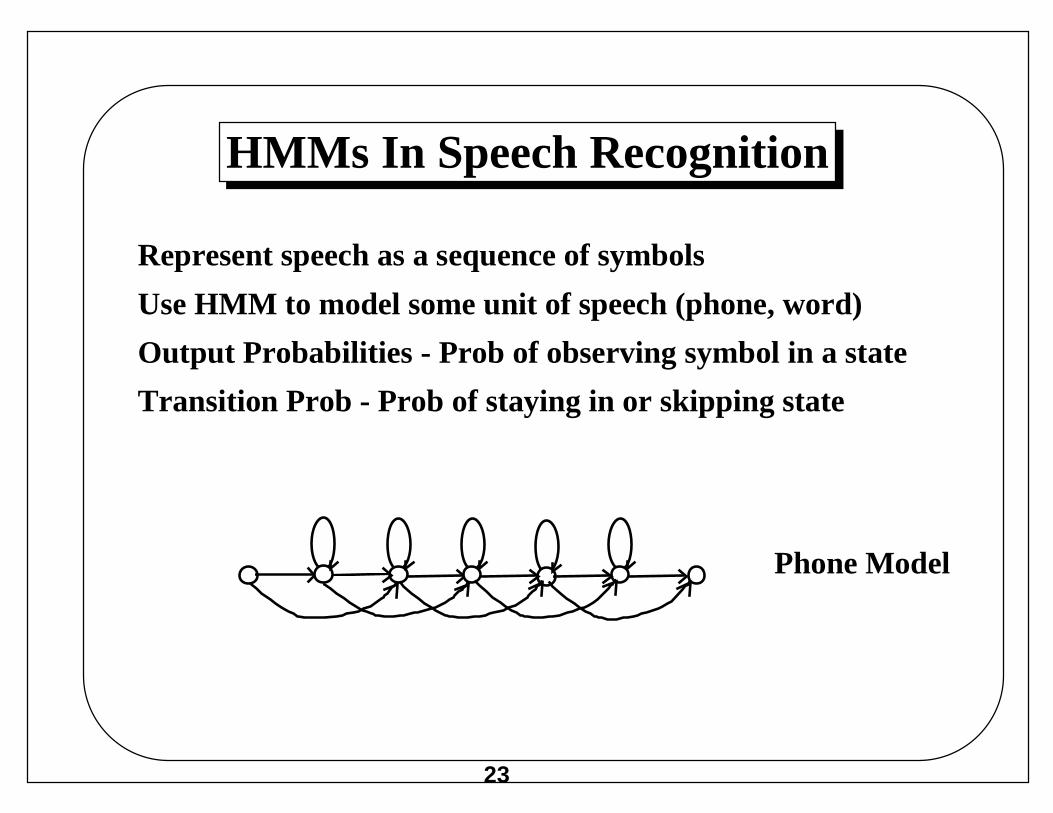
HMMs In Speech Recognition

Represent speech as a sequence of observations

Use HMM to model some unit of speech (phone, word)

Concatenate units into larger units

Phone Model

Word Modeld ih d

ih

11

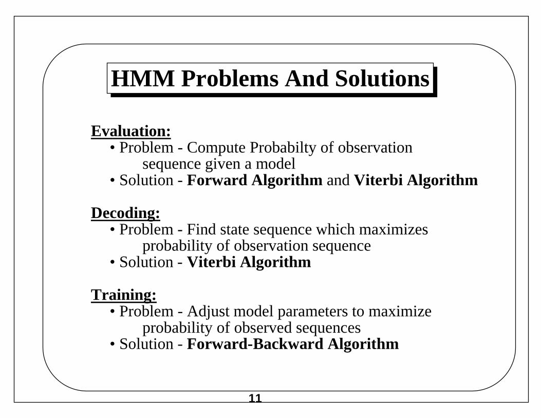
HMM Problems And Solutions

Evaluation:• Problem - Compute Probabilty of observation

sequence given a model• Solution - Forward Algorithm and Viterbi Algorithm

Decoding:• Problem - Find state sequence which maximizes

probability of observation sequence• Solution - Viterbi Algorithm

Training:• Problem - Adjust model parameters to maximize

probability of observed sequences• Solution - Forward-Backward Algorithm

12

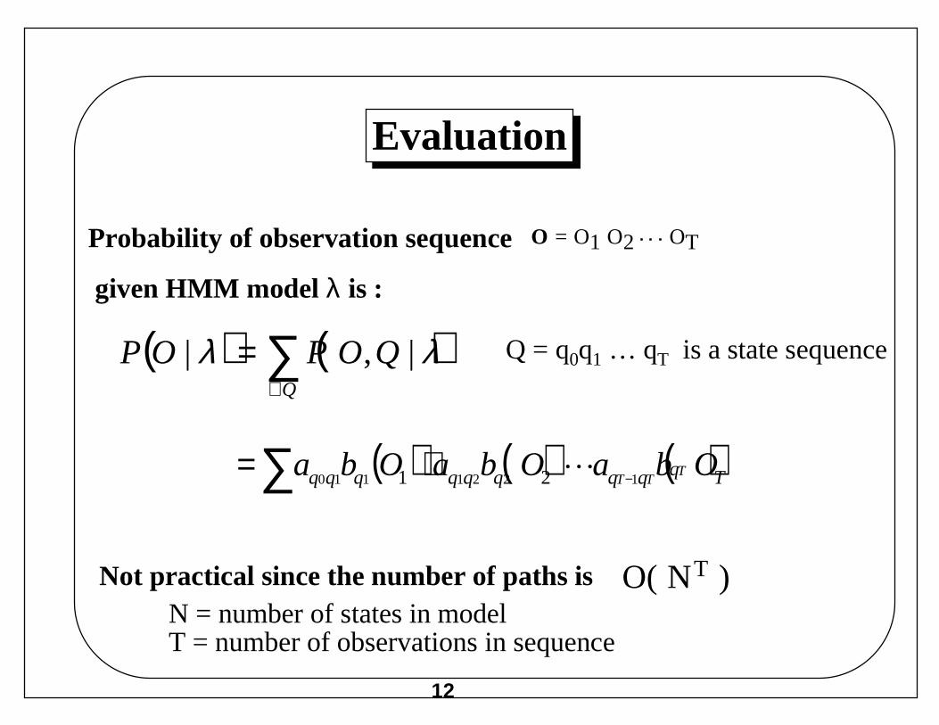
Evaluation

Probability of observation sequence

given HMM model λ is :

Not practical since the number of paths is O( NT )

Q = q0q1 … qT is a state sequence

O = O1 O2 OT

N = number of states in model T = number of observations in sequence

( ) ( ) |,| ∑∀

=Q

QOPOP λλ

( ) ( ) ( )Tqqqqqqqqq ObaObaOba TTT 1221110 21 −⋅=∑ L

13

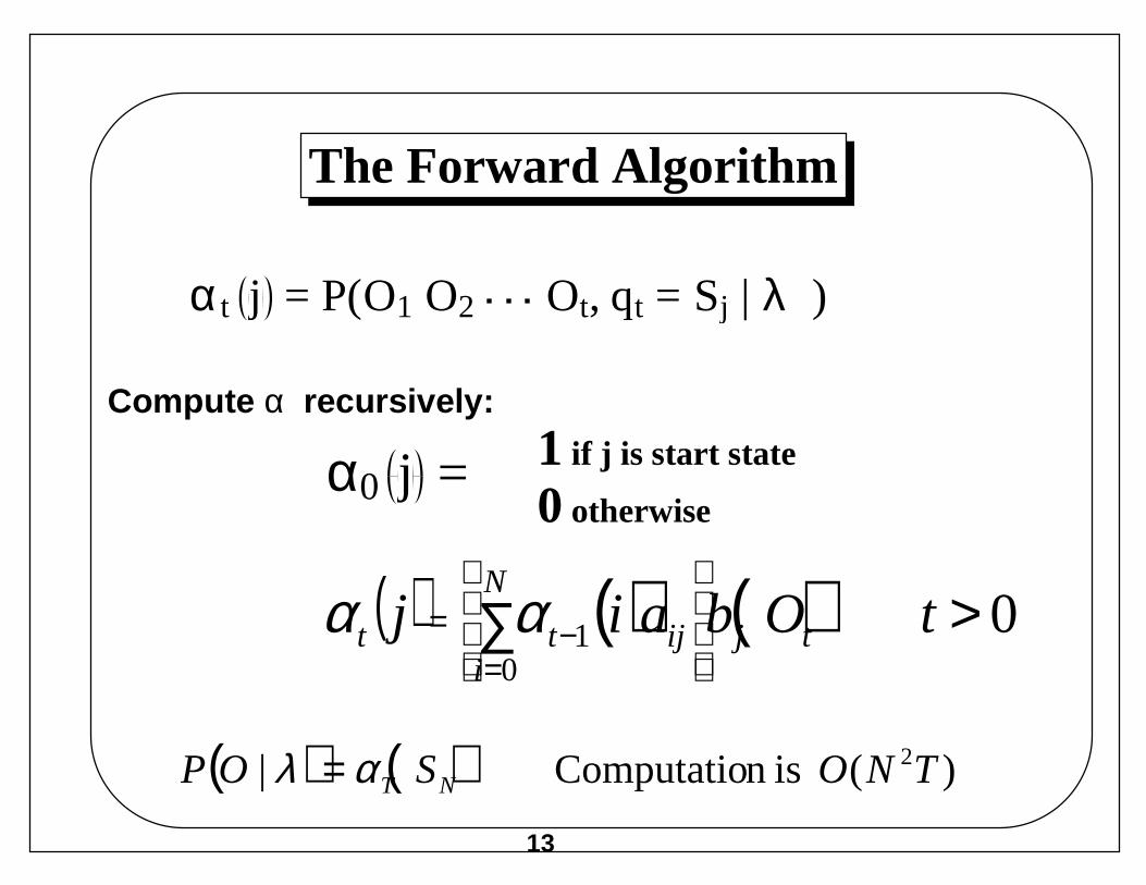
The Forward Algorithm

α t j = P(O1 O2 Ot, qt = Sj | λ )

Compute α recursively:

α 0 j = 1 if j is start state

0 otherwise

( ) ( ) ( ) 0 0

1 >∑

=−= tObaij tj

N

iijtt αα

( ) ( ) )( is nComputatio | 2TNOSOP NTαλ =

14

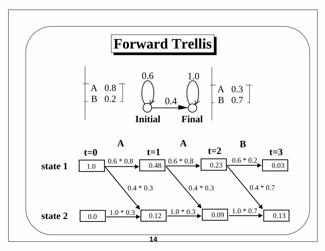
Forward Trellis

1.0state 10.6 * 0.8 0.6 * 0.8 0.6 * 0.2

0.0state 2 1.0 * 0.3 1.0 * 0.3 1.0 * 0.7

0.48 0.23 0.03

0.12 0.09 0.13

0.4 * 0.3 0.4 * 0.3 0.4 * 0.7

t=0 t=1 t=2 t=3A A B

A 0.8B 0.2

A 0.3B 0.7

Initial Final

0.6 1.0

0.4

15

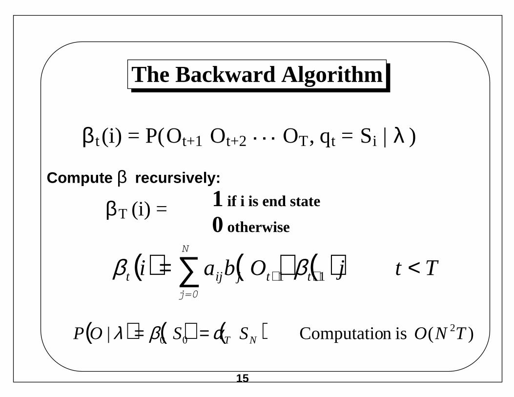
The Backward Algorithm

Compute β recursively:

1 if i is end state

0 otherwiseβ T (i) =

β t (i) = P(Ot+1 Ot+2 OT, qt = Si | λ )

( ) ( ) ( ) TtjObai ttjijt <= ∑ ++ 11 ββj=0

N

( ) ( ) ( ) )( is nComputatio | 200 TNOSSOP NTαβλ ==

16

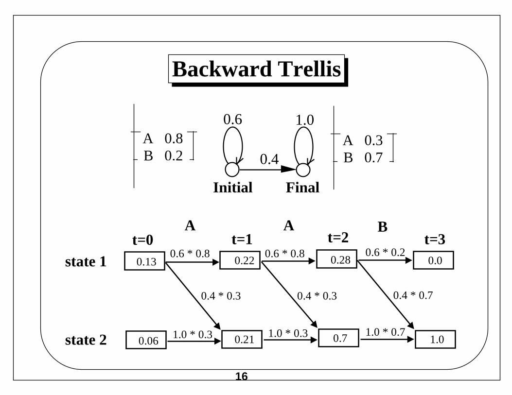
Backward Trellis

0.13state 10.6 * 0.8 0.6 * 0.8 0.6 * 0.2

0.06state 2 1.0 * 0.3 1.0 * 0.3 1.0 * 0.7

0.22 0.28 0.0

0.21 0.7 1.0

0.4 * 0.3 0.4 * 0.3 0.4 * 0.7

t=0 t=1 t=2 t=3A A B

A 0.8B 0.2

A 0.3B 0.7

Initial Final

0.6 1.0

0.4

17

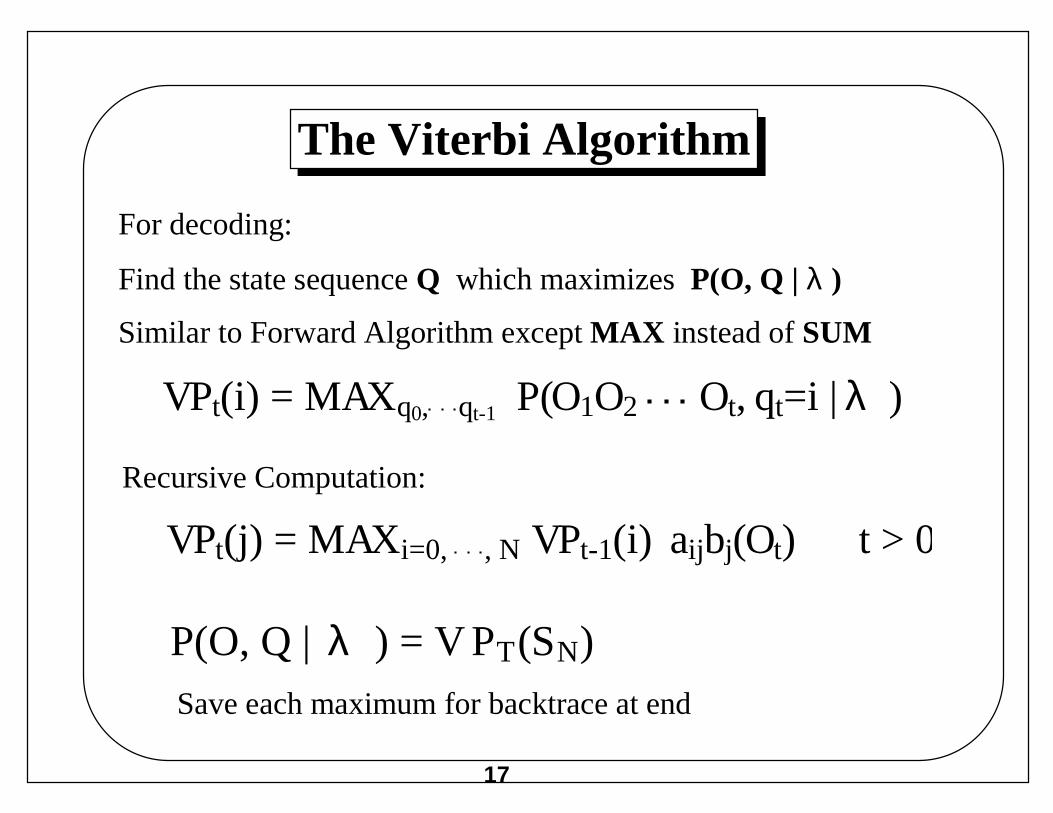
The Viterbi Algorithm

For decoding:

Find the state sequence Q which maximizes P(O, Q | λ )

Similar to Forward Algorithm except MAX instead of SUM

VPt(i) = MAXq0, qt-1 P(O1O2 Ot, qt=i | λ )

VPt(j) = MAXi=0, , N VPt-1(i) aijbj(Ot) t > 0

Recursive Computation:

Save each maximum for backtrace at end

P(O, Q | λ ) = V PT(SN)

18

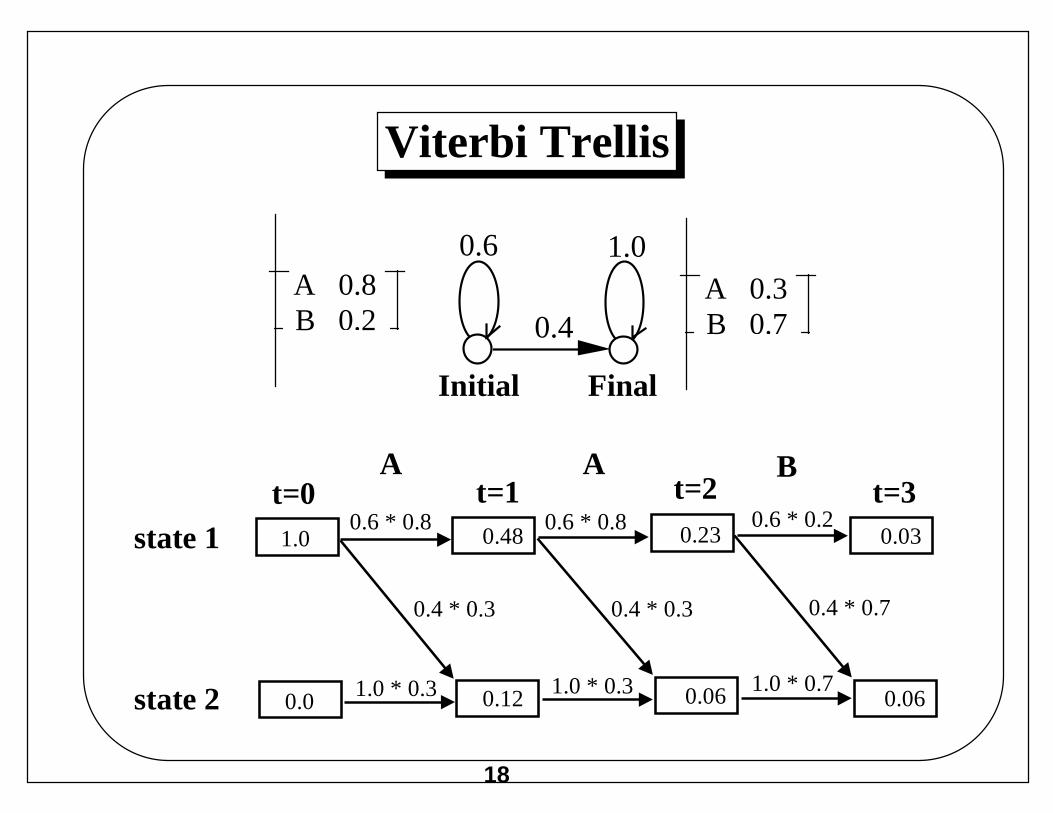
Viterbi Trellis

1.0state 10.6 * 0.8 0.6 * 0.8 0.6 * 0.2

0.0state 2 1.0 * 0.3 1.0 * 0.3 1.0 * 0.7

0.48 0.23 0.03

0.12 0.06 0.06

0.4 * 0.3 0.4 * 0.3 0.4 * 0.7

t=0 t=1 t=2 t=3A A B

A 0.8B 0.2

A 0.3B 0.7

Initial Final

0.6 1.0

0.4

19

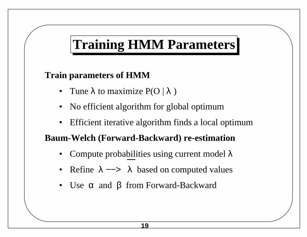
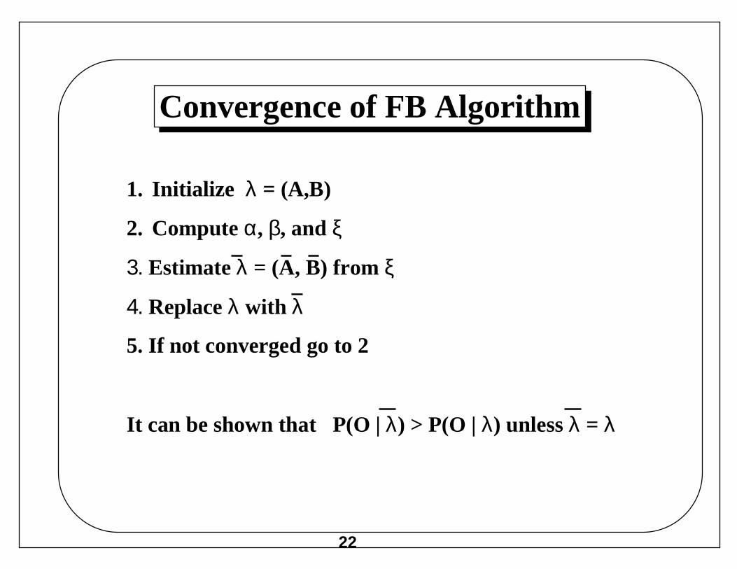
Training HMM Parameters

Train parameters of HMM

• Tune λ to maximize P(O | λ )

• No efficient algorithm for global optimum

• Efficient iterative algorithm finds a local optimum

Baum-Welch (Forward-Backward) re-estimation

• Compute probabilities using current model λ

• Refine λ −−> λ based on computed values

• Use α and β from Forward-Backward

20

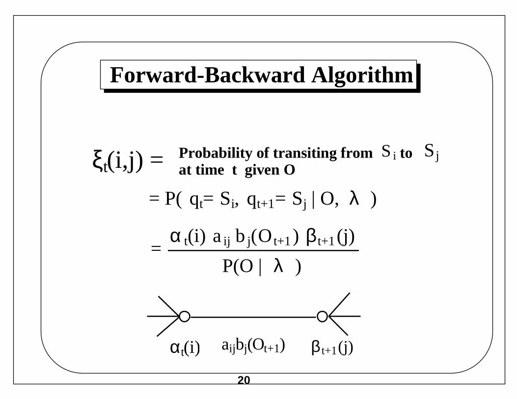
Forward-Backward Algorithm

Probability of transiting from toat time t given O

SjS i

= P( qt= Si, qt+1= Sj | O, λ )

= α t(i) a ij b j(Ot+1) β t+1 (j)

P(O | λ )

αt(i) aijbj(Ot+1) β t+1(j)

ξt(i,j) =

21

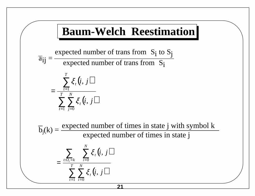
Baum-Welch Reestimation

bj(k) = expected number of times in state j with symbol kexpected number of times in state j

aij = expected number of trans from Si to Sj

expected number of trans from Si

( )

( )∑∑

∑

= =

==T

t

N

jt

T

tt

ji

ji

1 0

1

,

,

ξ

ξ

( )

( )∑ ∑

∑ ∑

= =

= ==T

t

N

it

kOt

N

it

ji

jit

1 0

: 0

,

,

ξ

ξ

22

Convergence of FB Algorithm

1. Initialize λ = (A,B)

2. Compute α, β, and ξ

3. Estimate λ = (A, B) from ξ

4. Replace λ with λ

5. If not converged go to 2

It can be shown that P(O | λ) > P(O | λ) unless λ = λ

23

HMMs In Speech Recognition

Represent speech as a sequence of symbols

Use HMM to model some unit of speech (phone, word)

Output Probabilities - Prob of observing symbol in a state

Transition Prob - Prob of staying in or skipping state

Phone Model

24

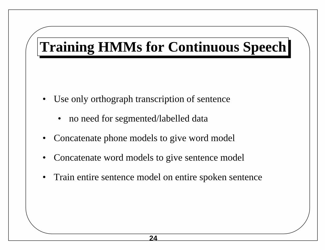
Training HMMs for Continuous Speech

• Use only orthograph transcription of sentence

• no need for segmented/labelled data

• Concatenate phone models to give word model

• Concatenate word models to give sentence model

• Train entire sentence model on entire spoken sentence

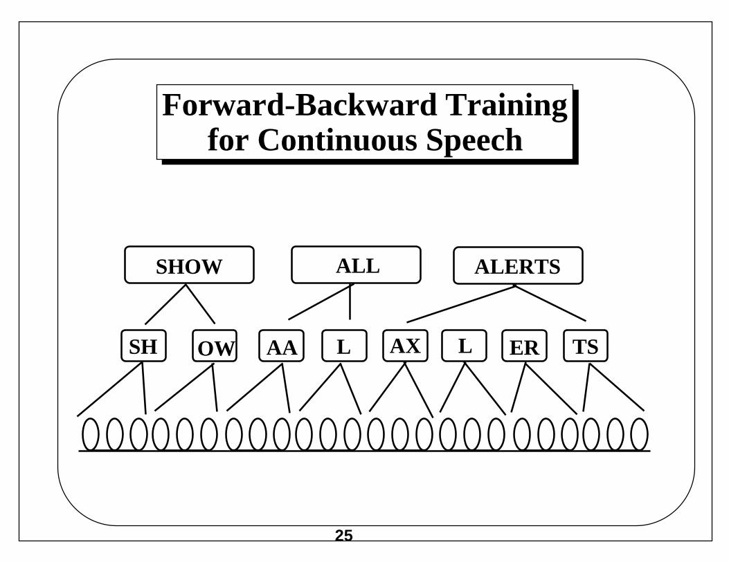
25

Forward-Backward Trainingfor Continuous Speech

SHOW ALL ALERTS

SH OW AA L AX L ER TS

26

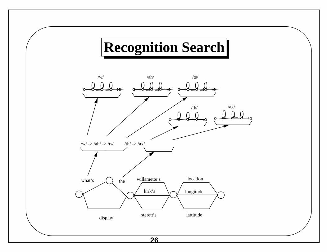
Recognition Search

/w/ -> /ah/ -> /ts/ /th/ -> /ax/

what’s the

display

kirk’s

willamette’s

sterett’s

location

longitude

lattitude

/w/ /ah/ /ts/

/th/ /ax/

27

Viterbi Search

• Uses Viterbi decoding

• Takes MAX, not SUM

• Finds optimal state sequence P(O, Q | λ )not optimal word sequence P(O | λ )

• Time synchronous

• Extends all paths by 1 time step

• All paths have same length (no need tonormalize to compare scores)

28

Viterbi Search Algorithm

0. Create state list with one cell for each state in system

1. Initialize state list with initial states for time t= 0

2. Clear state list for time t+1

3. Compute within-word transitions from time t to t+1

• If new state reached, update score and BackPtr

• If better score for state, update score and BackPtr

4. Compute between word transitions at time t+1

• If new state reached, update score and BackPtr

• If better score for state, update score and BackPtr

5. If end of utterance, print backtrace and quit

6. Else increment t and go to step 2

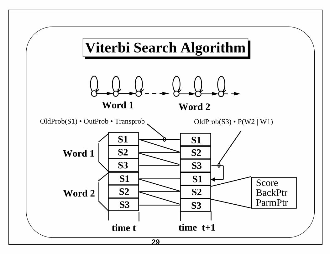
29

Viterbi Search Algorithm

Word 1 Word 2

time t time t+1

Word 1

Word 2

S1S2S3

S1

S1 S1S2S2

S2S3

S3 S3

OldProb(S1) • OutProb • Transprob OldProb(S3) • P(W2 | W1)

ScoreBackPtrParmPtr

30

Viterbi Beam Search

Viterbi Search

All states enumerated

Not practical for large grammars

Most states inactive at any given time

Viterbi Beam Search - prune less likely paths

States worse than threshold range from best are pruned

From and To structures created dynamically - list of active

states

31

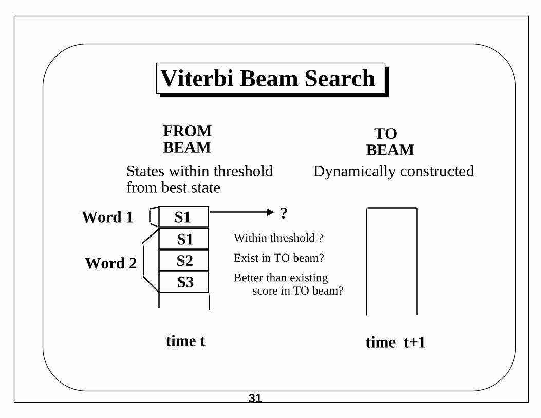
Viterbi Beam Search

time t time t+1

Word 1

Word 2

S1S1S2S3

FROMBEAM

TOBEAM

States within thresholdfrom best state

Dynamically constructed

?

Within threshold ?

Exist in TO beam?

Better than existingscore in TO beam?

32

Continuous Density HMMs

Model so far has assumed discete observations,each observation in a sequence was one of a set of Mdiscrete symbols

Speech input must be Vector Quantized in order toprovide discrete input.

VQ leads to quantization error

The discrete probability density bj(k) can be replacedwith the continuous probability density bj(x)where x is the observation vector

Typically Gaussian densities are used

A single Gaussian is not adequate, so a weighted sum ofGaussians is used to approximate actual PDF

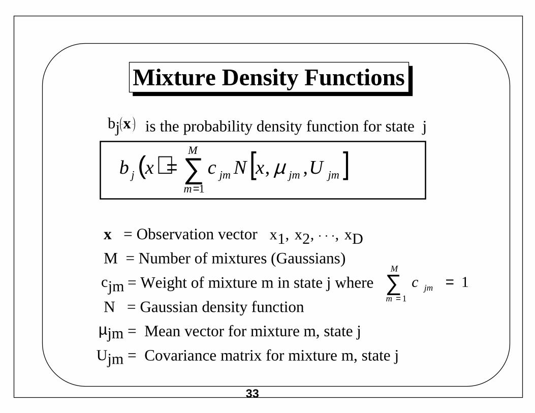
33

Mixture Density Functions

bj x is the probability density function for state j

x = Observation vector

M = Number of mixtures (Gaussians)

= Weight of mixture m in state j where

N = Gaussian density function

= Mean vector for mixture m, state j

= Covariance matrix for mixture m, state j

x1, x2, , xD

cjm

µjm

Ujm

( ) [ ]∑=

=M

mjmjmjmj UxNcxb

1

,, µ

11

=∑=

M

mjmc

34

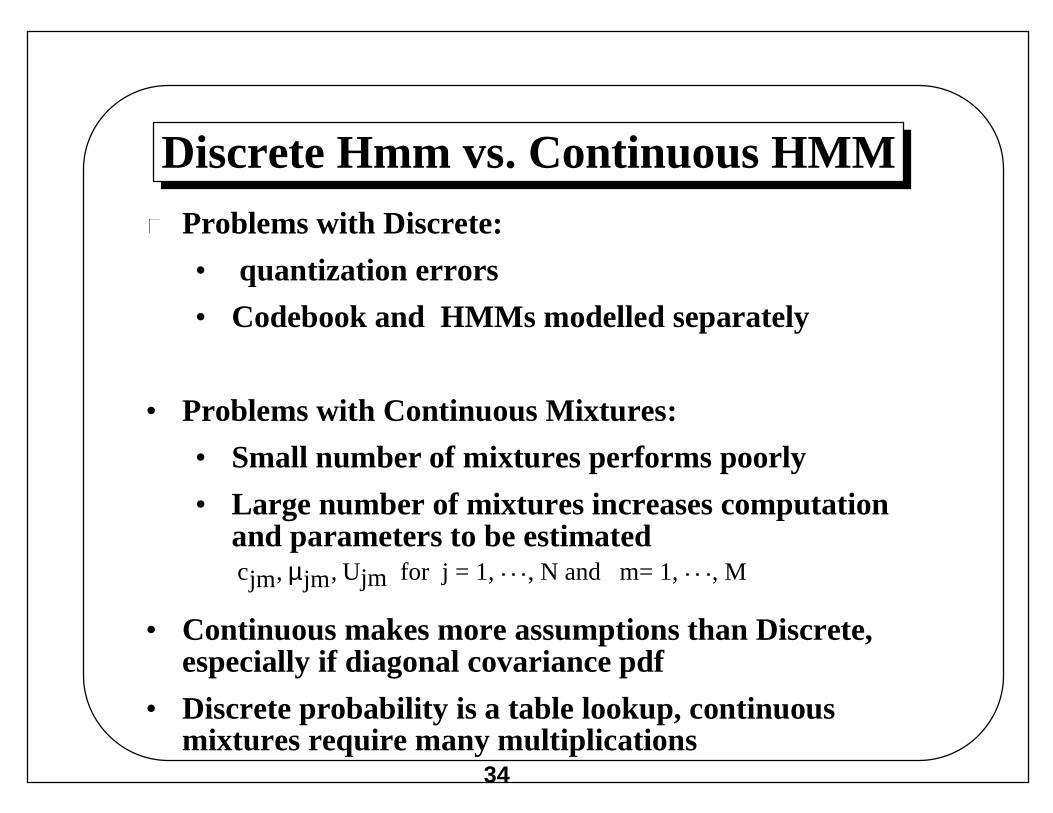
Discrete Hmm vs. Continuous HMM� Problems with Discrete:

• quantization errors

• Codebook and HMMs modelled separately

• Problems with Continuous Mixtures:

• Small number of mixtures performs poorly

• Large number of mixtures increases computationand parameters to be estimated

• Continuous makes more assumptions than Discrete,especially if diagonal covariance pdf

• Discrete probability is a table lookup, continuousmixtures require many multiplications

cjm, µjm, Ujm for j = 1, , N and m= 1, , M

35

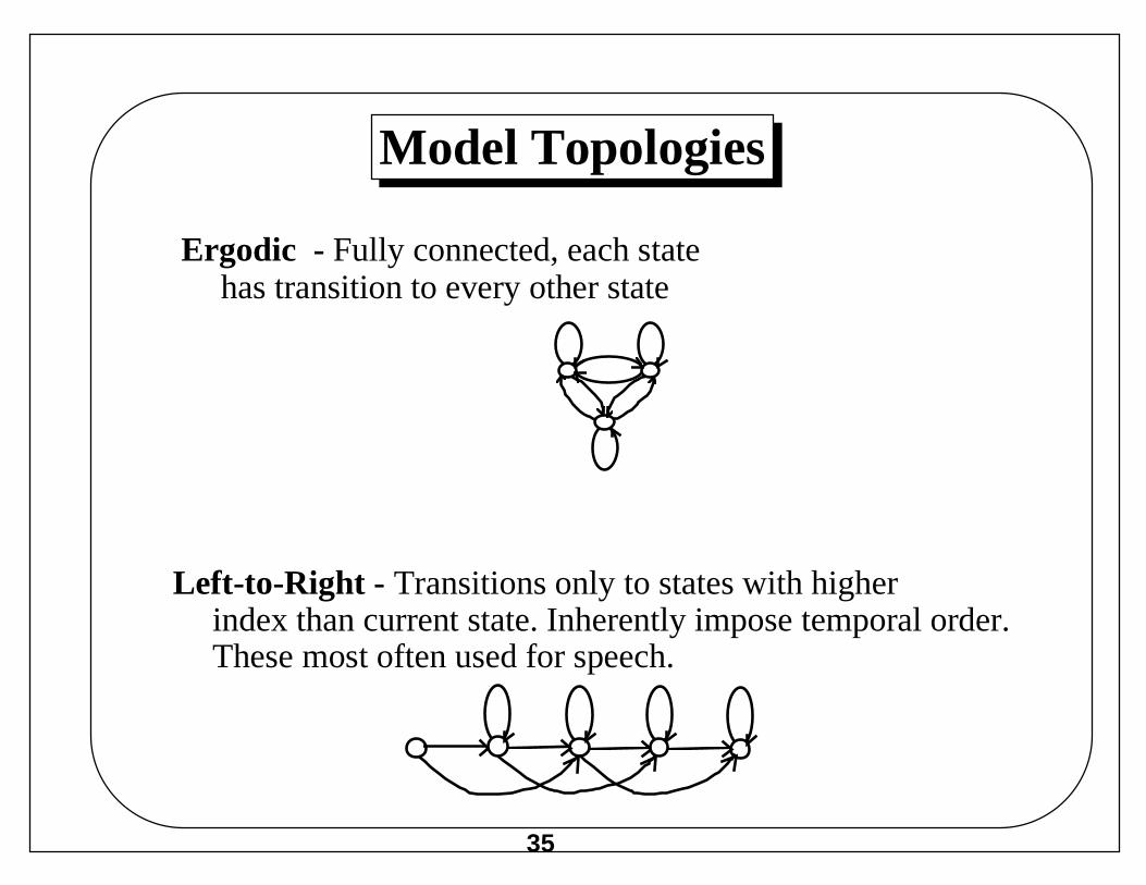
Model Topologies

Ergodic - Fully connected, each statehas transition to every other state

Left-to-Right - Transitions only to states with higherindex than current state. Inherently impose temporal order.These most often used for speech.